Probabilistic Hydrological Estimation of LandSlides (PHELS): global ensemble landslide hazard modelling

In this study we present a model for the global Probabilistic Hydrological Estimation of LandSlides (PHELS). PHELS estimates the daily hazard of hydrologically triggered landslides at a coarse spatial resolution of 36 km, by combining landslide susceptibility (LSS) and (percentiles of) hydrological variable(s). The latter include daily rainfall, a 7 d antecedent rainfall index (ARI7) or root-zone soil moisture content (rzmc) as hydrological predictor variables, or the combination of rainfall and rzmc. The hazard estimates with any of these predictor variables have areas under the receiver operating characteristic curve (AUC) above 0.68. The best performance was found with combined rainfall and rzmc predictors (AUC = 0.79), which resulted in the lowest number of missed alarms (especially during spring) and false alarms. Furthermore, PHELS provides hazard uncertainty estimates by generating ensemble simulations based on repeated sampling of LSS and the hydrological predictor variables. The estimated hazard uncertainty follows the behaviour of the input variable uncertainties, is about 13.6 % of the estimated hazard value on average across the globe and in time and is smallest for very low and very high hazard values.

1 Introduction

Landslides are mass movements of soil and rock triggered by anthropogenic or seismic activity and, most frequently, by rainfall (Froude and Petley, 2018; Nowicki Jessee et al., 2018; Stanley et al., 2021). In order to limit human and economic losses due to landslides, the prediction of where and when they are likely to occur is crucial (Crozier, 2013). The spatio-temporal probability of a landslide is generally referred to as “landslide hazard” and can be estimated based on a range of static environmental (spatial) and dynamic hydrological (temporal) data sources. The spatial and temporal information can either be merged directly, e.g. via machine learning techniques combining rainfall, soil moisture, snow and slope angle in an ad hoc fashion (Stanley et al., 2020, 2021), or in a two-step process that separately evaluates where and when landsliding is likely to occur (Kirschbaum and Stanley, 2018; Monsieurs et al., 2019a, b; Bordoni et al., 2020). The last approach is more common and traceable and requires that spatial and temporal probabilities are estimated individually before combining them into one prediction system.

The spatial probability, referred to as landslide susceptibility (LSS), is estimated based on (static) environmental features (Pourghasemi and Rossi, 2016; Reichenbach et al., 2018). Most LSS maps are created at the local to regional scale, where they are also used for mitigation and planning purposes (Guzzetti et al., 2005; Crozier, 2013). Others are specifically developed to be used in a landslide early warning system (Guzzetti et al., 2020) or “now-casting” approach: the global, categorized LSS assessment by Stanley and Kirschbaum (2017), for instance, has been developed to allow severity thresholds within the first version of the Landslide Hazard Assessment for Situational Awareness (LHASA) model (Kirschbaum and Stanley, 2018).

The temporal probability can either be calculated explicitly by physical models that compute the shear strength and stress in slopes (Lu and Godt, 2013; Baum et al., 2010) or approximated by statistical, empirical approaches (Guzzetti et al., 2008, 2020). The latter relate one or more dynamic hydrological predictor variables to a chance for a landslide (Guzzetti et al., 2008, 2020). A simple yet effective binary approach is to use thresholds for various measures of rainfall and soil water content beyond which landslide occurrence is expected (Segoni et al., 2018a). While univariate thresholds in antecedent rainfall index (ARI) or surface soil moisture exist (Kirschbaum and Stanley, 2018; Zhuo et al., 2019), most thresholds are based on two or more variables. The most frequently used thresholds are based on rainfall intensity and duration or variations thereof (Caine, 1980; Guzzetti et al., 2008; Rossi et al., 2017; Rosi et al., 2021) and hydrometeorological thresholds (Ponziani et al., 2012; Brocca et al., 2016; Devoli et al., 2018; Mirus et al., 2018; Thomas et al., 2019; Uwihirwe et al., 2020, 2022). Alternatively, it is possible to retrieve a continuous triggering probability based on rainfall (Calvello and Pecoraro, 2019), soil moisture measures (Wicki et al., 2020) or a combination of both (Bordoni et al., 2020). The measures of soil moisture range from antecedent soil moisture (Mirus et al., 2018; Wicki et al., 2020) and increase in soil saturation (Wicki et al., 2020) to soil moisture of the day (Bordoni et al., 2020) and refer to different soil layers (surface: Ponziani et al., 2012; Brocca et al., 2016; Thomas et al., 2019; Bordoni et al., 2020, root zone: Brocca et al. (2016); Mirus et al. (2018); Thomas et al. (2019); Wicki et al. (2020), groundwater: Uwihirwe et al. (2022)). In comparison to purely rainfall-based landslide likelihood predictions, the inclusion of soil water content has been found to prevent false alarms, independent of the data source (Ponziani et al., 2012; Segoni et al., 2018b; Mirus et al., 2018; Stanley et al., 2021).

To estimate hazard using the two-step process, the temporal probability assessment is combined with spatial LSS information. Monsieurs et al. (2019a, b) for example developed combined ARI–LSS thresholds. Kirschbaum and Stanley (2018) adapted the level of nowcasts (based on a global univariate ARI-threshold) according to LSS. Bordoni et al. (2020) updated LSS according to whether or not the temporal probability was above 0.5. We comprise all of the above-mentioned approaches under the term “hazard modelling”, while being aware that at smaller scales the size and mobility of a landslide may also be an essential part of hazard prediction.

The available landslide hazard modelling approaches rarely consider the quantification of uncertainty. For LSS, uncertainty information is sometimes provided (e.g. Broeckx et al., 2018, Depicker et al., 2020 and Felsberg et al., 2022b). For the temporal aspect, uncertainties have been assigned to rainfall and rainfall–LSS thresholds (Rossi et al., 2017; Monsieurs et al., 2019a). Hartke et al. (2020) created a probabilistic adaptation of the first version of LHASA by using rainfall distributions instead of deterministic values. This approach increased the number of correctly predicted landslides and decreased the number of false alarms from high nowcasts. For a physically based hazard estimate, Canli et al. (2018) proposed to use an ensemble of rainfall values as input, resulting in an ensemble of predicted hazard values.

In this study we (i) investigate the ability of different hydrological predictor variables for global landslide hazard estimation and (ii) use ensembles for an uncertainty assessment. We develop the Probabilistic Hydrological Estimation of LandSlides (PHELS) model. PHELS provides a global coarse-scale (36 km) dynamic landslide hazard simulation with a reliable uncertainty estimate at any time and location, by combining ensembles of LSS (Felsberg et al., 2022a, b) and daily information on hydrological predictor variables. For the latter, we test ensembles of rainfall and an ARI based on reanalysis precipitation data and root-zone soil moisture content [m³ m⁻³] (rzmc) from a land surface model. The paper is guided by the following research questions: (1) Which hydrological variable (or combination of variables) performs best at simulating global landslide hazards? (2) Is the estimated uncertainty related to the magnitude of the simulated hazard value?

2 Data, model and methods

2.1 Landslides

Despite the existence of many different types of landslides and their manifold shapes and sizes, in this study the term “landslide” refers to all types of hydrologically triggered mass movements. We use landslide data from the most recent version of the Global Landslide Catalog (GLC) (https://landslides.nasa.gov/viewer, last access: 20 January 2022). This inventory is based on media reports (Kirschbaum et al., 2010, 2015) and supplemented with the citizen science-based Landslide Reporter Catalog (LRC) data (Juang et al., 2019); see Stanley et al. (2021) for details. We select all landslides triggered by “continuous rain”, “downpour”, “monsoon”, “flooding”, “rain” and “tropical cyclone” (GLC classifiers). About 99 % of these landslides were collected in the time period 2007 through 2020. We therefore select this time period for the research conducted in this study. Note that the known economic and English-language bias, as well as the fact that media reports tend to focus on inhabited areas and landslides with notable impact on infrastructure, will affect the completeness of these inventories and reduce the reliability of their “absence reporting”.

Landslide information from the GLC was already successfully used for a number of global applications. Stanley and Kirschbaum (2017), Lin et al. (2017), and Felsberg et al. (2022b) used the locations of landslides to create global LSS maps. The first version of the global LHASA model was evaluated with landslide data from the GLC (Kirschbaum and Stanley, 2018), and LHASA version 2.0 was trained with a gridded GLC version (Stanley et al., 2021).

In this study, we additionally included 183 landslides from Russian quarterly reports (FSBIH, 2018; Felsberg et al., 2021) from 2010 to 2018, but for simplicity, we refer to the combined landslide dataset as “GLC”. Multiple landslide occurrences on one day within one grid cell are merged into one landslide event (LSE), resulting in a total number of 9367 LSEs for the study period as displayed in Fig. 1.

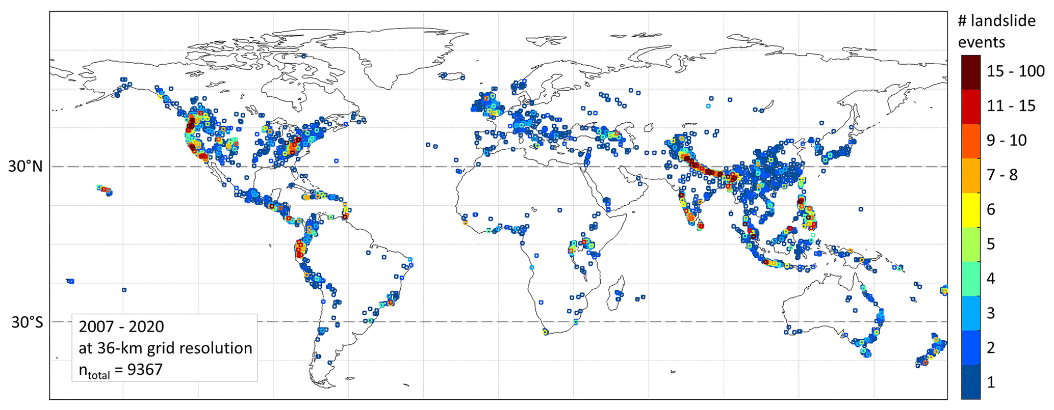
Figure 1 Spatial distribution of the number of reported landslide events per 36 km grid cell for the study period 2007 through 2020. Note the irregular colour bar intervals. Dashed grey lines indicate the latitude stratifications between “north”, “the tropics” and “south”.

2.2 Landslide susceptibility (LSS)

LSS describes the spatial likelihood of landslide occurrence (Crozier, 2013). In this study, we use the global LSS map of Felsberg et al. (2022a, b), developed on the 36 km Equal-Area Scalable Earth version 2 (EASEv2) grid for the purpose of subsequent combination with coarse-scale (satellite- or model-based) soil moisture data and with extended uncertainty assessment. This data-driven LSS focuses on hydrologically triggered landslides, and the most prominent predictor variables are the compound topographic index, long-term median surface soil moisture and evaporation, slope-related variables, and the peak ground acceleration. The LSS estimates consist of an ensemble of 2500 values per grid cell to reflect the LSS probability distribution. To facilitate subsequent flexible sampling from these ensembles, we fit a beta distribution ℬ_g(α_g,β_g) with shape parameters α_g,β_g to the 2500 ensemble LSS realizations at each grid cell g, using the package fitdistrplus of R version 4.0.3 (R Core Team, 2020) to estimate optimal parameters via maximum likelihood estimation.

2.3 Hydrological variables

To estimate the temporal likelihood of landslide occurrence, we use various hydrological predictor variables. We derive daily 36 km rainfall data (comprising convective and large-scale liquid precipitation) and the associated 7 d antecedent rainfall index (mm) (ARI7) from the global reanalysis data product Modern-Era Retrospective analysis for Research and Applications, Version 2 (MERRA-2) (Gelaro et al., 2017), available from 1980 onward. The ARI7 for day t was introduced by Kirschbaum and Stanley (2018) as a weighted (w_t) average of antecedent rainfall (r_t) during the preceding 7 d:

$$\begin{array}{}\text{(1)}& \mathrm{ARI}\mathrm{7}={\displaystyle \frac{{\sum }_{t=\mathrm{0}}^{\mathrm{6}}{r}_t\cdot w_t}{{\sum }_{t=\mathrm{0}}^{\mathrm{6}}{w}_t}},\mathrm{where}{w}_t=(t+\mathrm{1}{)}^{-\mathrm{2}}.\end{array}$$

The MERRA-2 data have a native spatial resolution of 0.625^∘ longitude × 0.5^∘ latitude and are interpolated to the 36 km EASEv2 grid via bilinear interpolation. These interpolated MERRA-2 data are also used as input to the state-of-the-art, physically based Catchment Land Surface Model (CLSM) (Koster et al., 2000) to simulate rzmc [m³ m⁻³] (0–100 cm) for the study period. The rzmc contains information on both surface water content and groundwater and should therefore be indicative not only of water content at landslide shear planes <1 m, which we consider a typical depth, but also for more shallow or deep-seated landslides.

CLSM simulations are run with 24 ensemble members by perturbing meteorological input (including rainfall) and select state variables (see Felsberg et al., 2021). The resulting ensemble average of rainfall and rzmc is used for deterministic hazard modelling, whereas the ensemble average and standard deviation are used to sample input values for the ensemble hazard modelling.

In a next step, the sampled hydrological variables are transformed into percentiles to detach their magnitudes from the local climatological conditions. Felsberg et al. (2021) moreover found that the transformation into percentiles of soil water content enhanced the ability to distinguish between LSE and sampled days with no landslide event (noLSE). The climatological percentile thresholds are computed per grid cell based on long-term (entire study period 2007–2020) time series of ensemble mean simulations of soil water content, similar as in Felsberg et al. (2021).

2.4 The PHELS model

The objective of PHELS is to obtain a measure of landslide hazard in a probabilistic way. The probability of landslide event occurrence (LSE =1) given static environmental conditions or dynamic variables x_i can be described stochastically through conditional probabilities $p(\mathrm{LSE}=\mathrm{1}\mid x_i)$ (van Westen et al., 2006; Calvello and Pecoraro, 2019; Uwihirwe et al., 2020; Lombardo et al., 2020; Felsberg et al., 2021). For the static condition we use LSS (x_L), and for the dynamic variable we use percentiles of daily rzmc, rainfall and ARI7 describing the hydrological conditions (x_h). The probability of a landslide event occurring conditioned on the susceptibility of the location and the hydrological state of the day can be defined as follows using Bayes' law:

$$\begin{array}{}\text{(2)}& \begin{array}{rl}p(\mathrm{LSE}& =\mathrm{1}\mid x_{\mathrm{L}},x_{\mathrm{h}})\\ & ={\displaystyle \frac{p(x_{\mathrm{L}},x_{\mathrm{h}}\mid \mathrm{LSE}=\mathrm{1})\cdot p(\mathrm{LSE}=\mathrm{1})}{p(x_{\mathrm{L}},x_{\mathrm{h}})}}\end{array},\end{array}$$

or if two hydrological variables are taken into account,

$$\begin{array}{}\text{(3)}& \begin{array}{rl}p(\mathrm{LSE}& =\mathrm{1}\mid x_{\mathrm{L}},x_{\mathrm{h}\mathrm{1}},x_{\mathrm{h}\mathrm{2}})\\ & ={\displaystyle \frac{p(x_{\mathrm{L}},x_{\mathrm{h}\mathrm{1}},x_{\mathrm{h}\mathrm{2}}\mid \mathrm{LSE}=\mathrm{1})\cdot p(\mathrm{LSE}=\mathrm{1})}{p(x_{\mathrm{L}},x_{\mathrm{h}\mathrm{1}},x_{\mathrm{h}\mathrm{2}})}}\end{array}.\end{array}$$

Bayes' theorem connects the prior probability p(LSE=1) with a known likelihood function of the conditions $p(x_{\mathrm{L}},x_{\mathrm{h}}\mid \mathrm{LSE}=\mathrm{1})$ to obtain a posterior probability. While LSS could conceptually be considered a prior probability, we opt to use it as a temporally static (but spatially varying) variable and implement it as a condition in a similar way as the temporally dynamic soil moisture, ARI7 and rainfall. In this study, p(LSE=1) thus remains an uninformative prior, which is assumed constant in space and time. Since we use percentiles of rzmc, rainfall and ARI7 as hydrological predictor variables, their respective distributions are (quasi-)uniform, but their joint probability is not necessarily uniform. Nevertheless, for simplicity, we omit the normalizing joint probability terms and use the following proportionality approach:

$$\begin{array}{}\text{(4)}& \begin{array}{rl}p(\mathrm{LSE}& =\mathrm{1}\mid x_{\mathrm{L}},x_{\mathrm{h}})\propto p(x_{\mathrm{L}},x_{\mathrm{h}}\mid \mathrm{LSE}=\mathrm{1})\\ & \Rightarrow \mathcal{H}=f(x_{\mathrm{L}},x_{\mathrm{h}}),\end{array}\end{array}$$

or for multiple hydrological variables $\mathcal{H}=f(x_{\mathrm{L}},x_{\mathrm{h}\mathrm{1}},x_{\mathrm{h}\mathrm{2}})$, i.e. a function of the predictor variables x_L, x_h1 and x_h2. We refer to this posterior probability value as landslide hazard [−] (ℋ). By foregoing the normalization, and because the absolute values of the distribution fits (below) depend on the binning and dimensions (scale) of the underlying data, the absolute values of ℋ with one or two hydrological variables will not be comparable. However, for hazard estimation, only a relative spatio-temporal assessment is of importance.

To estimate $p(x_{\mathrm{L}},x_{\mathrm{h}}\mid \mathrm{LSE}=\mathrm{1})$, we extract values of LSS and the hydrological variables for the 9367 LSE. Figure 2a shows the bivariate histogram for percentiles of rzmc, with the number of LSE indicated in colour. Distributions for the other hydrological variables (not shown) generally exhibit the same behaviour: LSEs are exponentially more likely to occur where LSS is high and under wet hydrological conditions, both individually and combined. At the same time, low LSS or drier conditions do not exclude the possibility of landslide occurrence. We find that 1.8 %/1.3 %/0.7 % of the LSE occurs where LSS is below 0.5 [−] and percentiles of rzmc/rainfall/ARI7 are below 50 [−]. For very susceptible locations, LSEs also occur at much drier hydrological conditions, whereas very wet conditions still require a certain level of LSS. This results in a skewing of the distribution from the upper right towards the upper left corner, which was also observed by Monsieurs et al. (2019a).

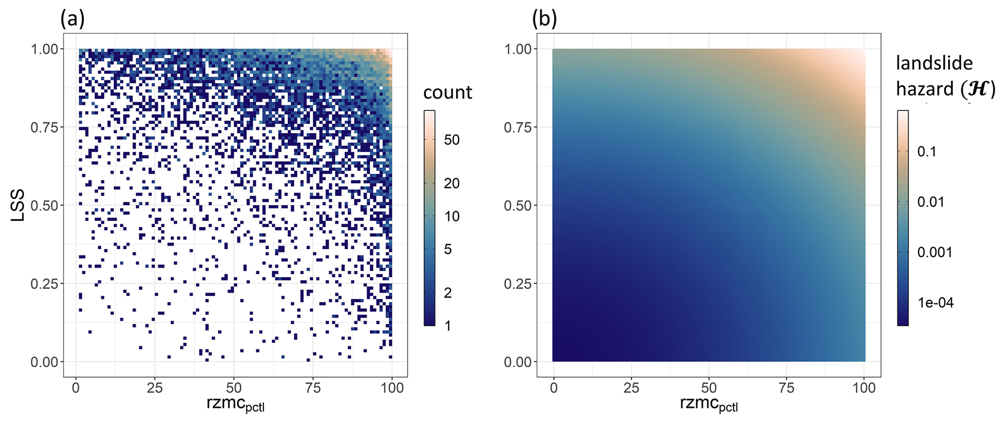
Figure 2 (a) Bivariate histogram of daily percentiles of rzmc (rzmc_pctl) and LSS for landslide events between 2007 and 2020. These data were used to fit the bivariate exponential of Eq. (5). (b) Hazard (ℋ [−]) as a bivariate exponential fitted function of daily rzmc_pctl and LSS. Note the logarithmic colour bar intervals.

Next, a two- or three-dimensional quadratic–exponential function is fit through the extracted LSE data. This kind of fit through the distribution of data points is a long-term and spatially aggregated summary statistic, also referred to as system signature (Vrugt and Sadegh, 2013). We tested different forms of the fitting equation and found the lowest root mean squared deviation (relative to the entire observed LSE distribution) for the following exponential functions with one and two hydrological predictor variables, respectively:

$$\begin{array}{}\text{(5)}& \mathcal{H}=a\cdot \exp (b\cdot x_{\mathrm{L}}^{\mathrm{2}}+c\cdot x_{\mathrm{h}}^{\mathrm{2}})\end{array}$$

and

$$\begin{array}{}\text{(6)}& \mathcal{H}=a\cdot \exp (b\cdot x_{\mathrm{L}}^{\mathrm{2}}+c\cdot x_{\mathrm{h}\mathrm{1}}^{\mathrm{2}}+d\cdot x_{\mathrm{h}\mathrm{2}}^{\mathrm{2}}).\end{array}$$

These equations are the core of the PHELS model. Ensuring ${\sum }_{x_{\mathrm{L}},x_{\mathrm{h}}}\mathcal{H}\equiv \mathrm{1}$ for $x_{\mathrm{L}}\in \mathit{\{}\mathrm{0},\mathrm{0.01},\mathrm{\dots },\mathrm{1}\mathit{\}}$ (binned continuous values) and $x_{\mathrm{h}}\in \mathit{\{}\mathrm{1},\mathrm{2},\mathrm{\dots },\mathrm{100}\mathit{\}}$ (percentiles, discrete) results in the parameters shown in Table 1. Note that ensuring the sum of 1 only offsets the scaling factor a and does not affect the other parameters. For the fitting (“nls”) and summing, we use R version 4.0.3 (R Core Team, 2020), and optimal parameters are obtained by minimizing the residual sum of squares between observed and fitted counts.

Table 1 Parameters of the exponential fit (Eqs. 5 and 6) for PHELS based on different hydrological variables (columnwise). Parameters are given for the static x_L (parameter b) and one hydrological variable x_h (parameter c for rzmc, rainfall or ARI7) or two hydrological variables x_h1,x_h2 namely rzmc (parameter c) and rainfall (parameter d). To simplify comparison between parameters b, c and d across the different orders of magnitudes ($\mathcal{O}\left(x_{\mathrm{L}}^{\mathrm{2}}\right)=\mathrm{1}$ and $\mathcal{O}\left(x_{\mathrm{h}}^{\mathrm{2}}\right)=\mathrm{10}\mathrm{000}$), c and d are shown as multiples of 10⁻⁴. Residual standard errors are shown for all fits, as well as the theoretical maximum hazard values ${\mathcal{H}}_{\max }=\mathcal{H}(x_{\mathrm{L}}=\mathrm{1},x_{\mathrm{h}}=\mathrm{100})$ and ${\mathcal{H}}_{\max }=\mathcal{H}(x_{\mathrm{L}}=\mathrm{1},x_{\mathrm{h}\mathrm{1}}=\mathrm{100},x_{\mathrm{h}\mathrm{2}}=\mathrm{100})$, respectively. Note that the absolute ℋ values are not to be compared for PHELS models with varying numbers of input variables.

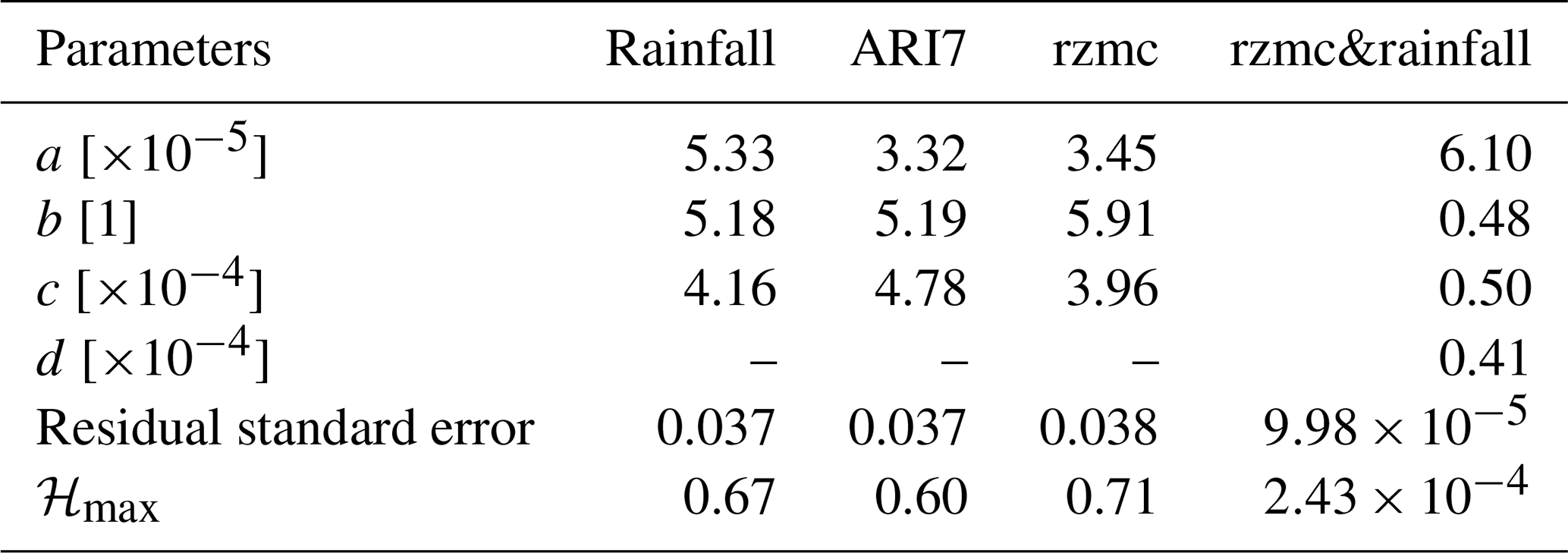
The difference between the parameters b and c for $x_{\mathrm{L}}^{\mathrm{2}}$ and $x_{\mathrm{h}}^{\mathrm{2}}$ reflects the observed skew in the bivariate histogram. The skew in ℋ is most pronounced as a function of rzmc, reduces for rainfall and is least for ARI7. When having both rzmc and rainfall as hydrological predictor variables (referred to as rzmc&rainfall), rzmc and LSS become equally important and rainfall slightly less. This indicates that both LSS and soil wetness are necessary preconditions for LSE occurrence. The different order of magnitude in the parameters of PHELS based on Eqs. (5) and (6) is a result of extending the quadratic exponential to a third predictor variable. Retaining the integral of 1 over the predictor space moreover reduces the magnitude of resulting ℋ from maximum values of ∼ 0.7 to 0.00024 (see Table 1). This effect can be avoided by using the complete Bayesian theorem as in Eqs. (2)–(3) with inclusion of a normalization of the probability instead of the proportionality approach of Eq. (4). The average residual standard error is ∼ 0.04 when using only rzmc, rainfall or ARI7 as predictors along with LSS, and the error is relatively larger when two hydrological variables are included. This is because a multidimensional fit is harder to achieve (more variation to account for). Nevertheless, the resulting distribution of ℋ as shown in Fig. 2b for rzmc percentiles represents the observed patterns (Fig. 2a) well.

PHELS estimates can be obtained for single values of the hydrological predictor variables and LSS. Such PHELS estimates are referred to as deterministic ℋ. In order to propagate uncertainties of these input variables, PHELS can also be run as an ensemble with members $i=\mathrm{1},\mathrm{\dots },N_{\mathrm{ens}}$. Figure 3 illustrates this approach for one grid cell (g) at one time step (t [days]) for ℋ based on rzmc, rainfall and LSS. First, we sample LSS from the beta distribution ℬ_g(α_g,β_g) and obtain $x_{\mathrm{L},g,i}$. Next, we sample rzmc${}_{g,t,i}$ from a normal distribution where μ_g,t and σ_g,t are the rzmc ensemble average and standard deviation diagnosed from 24 ensemble CLSM simulations. The sampled rzmc${}_{g,t,i}$ is subsequently transformed into the corresponding percentile by comparison against long-term percentile thresholds for this grid cell and used as $x_{\mathrm{h},g,t,i}$ from Eq. (5) or as $x_{\mathrm{h}\mathrm{1},g,t,i}$ from Eq. (6). The same way of sampling is used for rainfall or ARI7. Applying Eq. (6) to $x_{\mathrm{L},g,i=\mathrm{1}}$, $x_{\mathrm{h}\mathrm{1},g,t,i=\mathrm{1}}$ and $x_{\mathrm{h}\mathrm{2},g,t,i=\mathrm{1}}$ yields the first hazard ensemble member ${\mathcal{H}}_{g,t,i=\mathrm{1}}$. The sampling is repeated N_ens=100 times to retrieve a landslide hazard ensemble (ℋ_ens). This allows us to obtain an ensemble average ℋ ($\stackrel{\mathrm{‾}}{\mathcal{H}}$) with a connected uncertainty (ensemble standard deviation). Note that all ensemble sampling was performed independently in time and for each variable, without accounting for temporal autocorrelations or cross-correlations between variables. During hydrological extreme events such as tropical storms, this may result in conservatively high ℋ uncertainty estimates in comparison to sampling from multidimensional distributions of the hydrological variables (not shown). PHELS is coded in R version 4.0.3 (R Core Team, 2020). A 1 d simulation of the global ℋ_ens with N_ens=100 at 36 km spatial resolution takes ∼ 5 min on one core.

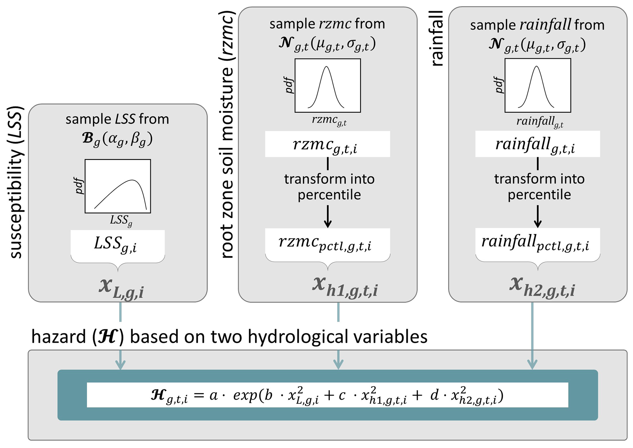
Figure 3 Schematic of the sampling setup within PHELS for the example of combined hydrological predictor variables rzmc&rainfall. i refers to the ensemble member, g to the grid cell and t to the time [days]. Percentiles of rzmc and rainfall on day t are used to derive hazard estimates ℋ for the same day following Eq. (6). μ and σ are the ensemble average and standard deviation. The transformation into percentiles is achieved by comparing rzmc${}_{g,t,i}$ and ${\mathrm{rainfall}}_{g,t,i}$ against long-term percentile thresholds of the corresponding grid cell g.

2.5 Evaluation

The evaluation of PHELS is performed both for deterministic and ensemble ℋ estimates. The strength of PHELS is that it provides relative estimates of hazards in both space and time. However, given the known strong spatial performance of the LSS (Felsberg et al., 2022b), the focus will be on a conservative evaluation of the performance in time.

More specifically, the PHELS hazard results are evaluated at grid cells and days of LSE for the study period (2007–2020, n_total=9367). For grid cells with at least one LSE, we randomly sample an equal number of values for noLSE from all other time steps. In order to account for possible errors in the date reporting and time zone matching of observations and hydrological data (local time versus UTC), 3 d prior and after an LSE are excluded from the selection as noLSE. For the same reasons we also evaluate the performance for maximum hazard values within a 3 d window around the LSE (±1 d, “LSE3”) as was done by Kirschbaum and Stanley (2018) and Monsieurs et al. (2019a). To evaluate the full spatio-temporal performance, we moreover test the performance when n_total noLSEs are randomly sampled across the globe and in time, without restriction to the LSE grid cells (“noLSEglobal”).

We evaluate the performance of the PHELS models with various hydrological predictor variables (rzmc, rainfall, ARI7 and rzmc&rainfall). The resulting ℋ is compared for LSE and noLSE in terms of receiver operation characteristic (ROC) curve, where the true positive rate (TPR) is plotted against the false positive rate (FPR) for different thresholds in the continuous probability values of ℋ. The TPR is the ratio of correctly predicted LSE (“true positives”) to the total number of LSE (Wilks, 2011). An LSE is assumed to be predicted when the probability is above a set threshold. The FPR is the ratio of erroneously predicted LSE (“false positives”) to the total number of noLSE, here being the same as LSE due to our 1:1 ratio of sampling. For a perfect prediction, the area under the ROC curve (AUC) is 1. A value of 0.5 on the other hand indicates that the prediction is not better than a uniform random prediction. We conduct the ROC analysis for the full data sets of LSE and noLSE, and for LSE3 and noLSEglobal, as well as subsets stratified for latitude and season. Latitudes are stratified at 30^∘ N and 30^∘ S into “north”, the “tropics” and “south”, as indicated by the dashed lines in Fig. 1. Note that the “south” subset contains much less data. Stratification for seasons follows meteorological standards, i.e. December–January–February (DJF), March–April–May (MAM), June–July–August (JJA) and September-October-November (SON). For additional insight, we compare numbers of false predictions, i.e. false alarms (“false positives”) and missed alarms (“false negatives”) for the LSE grid cells only. We set the 90th percentile of ℋ within one grid cell over all time steps as a threshold to distinguish between predicted positive and negative.

3 Results

3.1 Deterministic hazard estimates

Figure 4 shows time series of PHELS ℋ in a grid cell near Seattle, USA, based on different ensemble mean predictor variables as deterministic input. For rainfall, fast changes at rainfall events induce a spiky pattern with frequent short-term changes in ℋ. For ARI7 fewer spikes are visible and the rainy season stands out more. Seasonal patterns are even more pronounced for rzmc reflecting longer-term transitions, while the signal of the rainfall event spikes is strongly dampened. ℋ based on rzmc&rainfall shows both the general long-term seasonality and short-term spikes of rainfall events. In this grid cell, LSEs usually coincide with peaks or higher values in simulated ℋ. The first LSE in autumn 2014 coincides with a peak in ℋ based on rainfall and ARI7. Based on rzmc, ℋ is however very small and would have resulted in a missed alarm. The opposite is the case for two LSEs in March 2015 where ℋ based on rzmc is still elevated, but close to zero for rainfall and ARI7. When based on rzmc&rainfall, both examples show elevated ℋ.

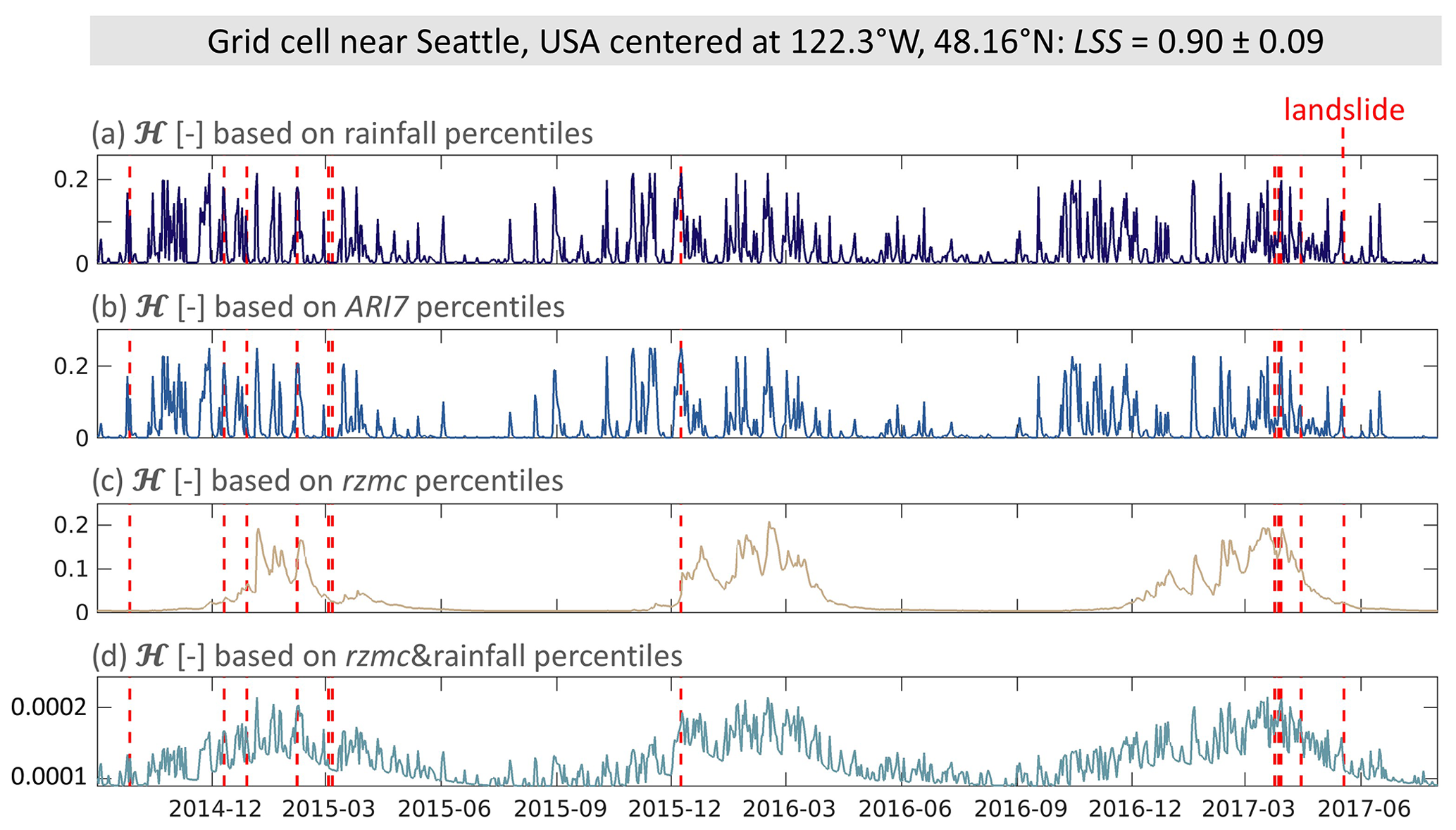
Figure 4 Time series of daily PHELS hazard (ℋ [−]) based on different hydrological predictor variables for a grid cell near Seattle, USA. ℋ is based on percentiles of (a) rainfall, (b) ARI7, (c) rzmc and (d) rzmc&rainfall. Note the different scale in magnitude for (d). Days with LSE are indicated by the dashed red lines.

Figure 5 shows ROC curves for ℋ estimates from PHELS with different hydrological predictor variables, yielding AUC values between 0.68 and 0.79, only for grid cells with at least one LSE in their time history, and only considering the ℋ estimates at the exact days of the LSE and noLSE samples. ℋ based on rzmc&rainfall performs better than based on one single hydrological variable, closely followed by ℋ based on ARI7 (difference of only 0.02).

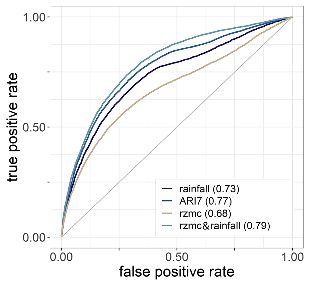
Figure 5 ROC curves for PHELS ℋ simulations using one hydrological variable (rainfall, ARI7, rzmc) or both rzmc&rainfall based on the original LSE and noLSE samples, i.e. for the reported dates and only within LSE grid cells. AUC values are indicated in brackets.

To disentangle these differences in performance, Fig. 6 shows AUC values for different subsets of the LSE–noLSE validation data per latitude and season. The best performance is typically found for the subset MAM–south across all hydrological variables. The second best performance is found during DJF–north for rainfall, ARI7 and rzmc&rainfall and during DJF–tropics for rzmc. In general, ℋ based on rzmc performs above average for the tropics throughout all seasons. Apart from JJA–tropics based on rzmc, performances for JJA are below average across all predictor variables and latitude stratifications. During spring time (MAM–north, SON–south), rainfall and ARI7 performances are largely below average, rzmc performance is closer to the average and for rzmc&rainfall performance is average.

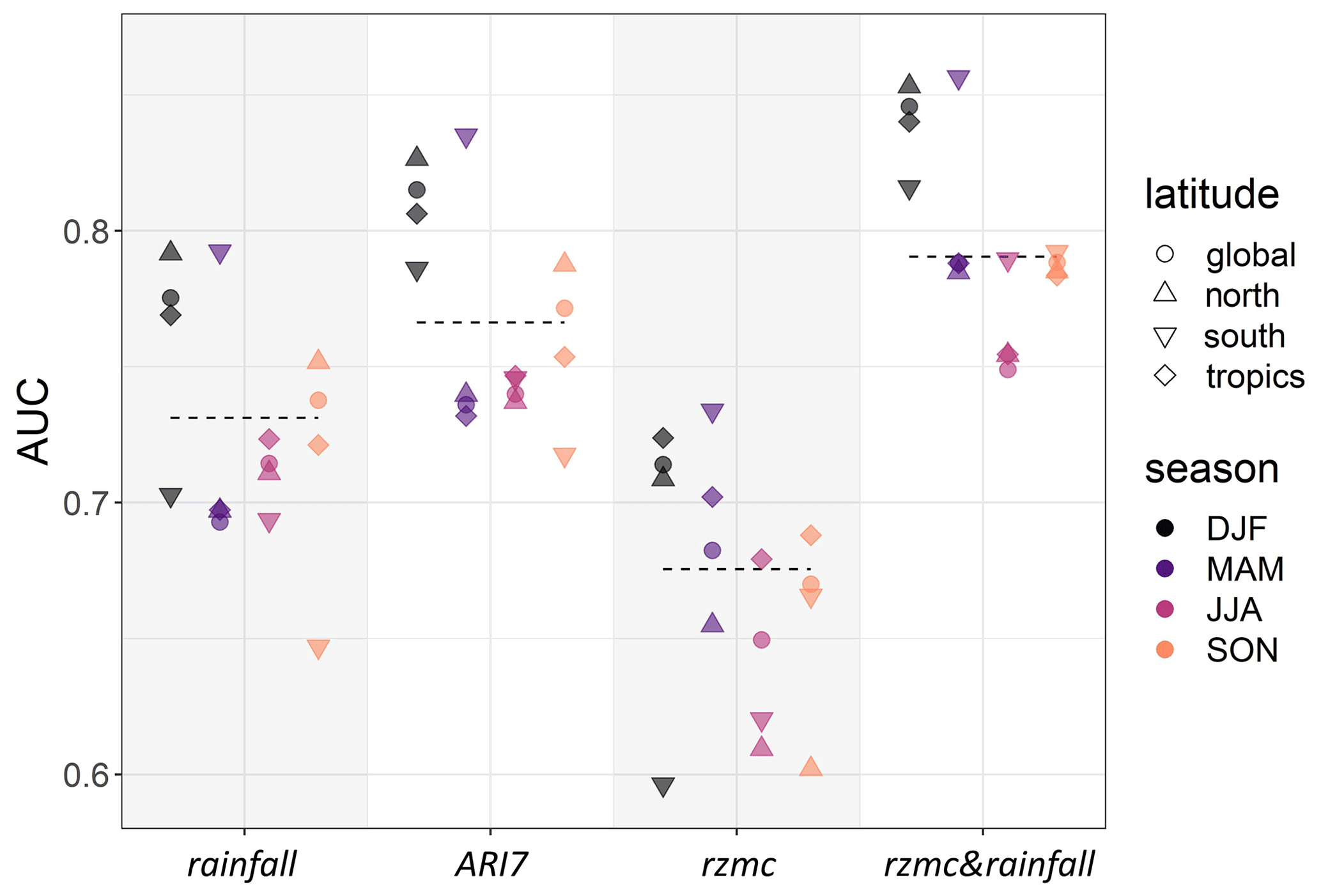
Figure 6 AUC values for PHELS hazard stratified per latitude and season, for the different hydrological predictor variables. AUC of the full data is indicated by the horizontal dashed line. Season stratifications are shown from left to right (and dark to light colour) per predictor variable: DJF, MAM, JJA and SON. This AUC analysis is based on the LSE and noLSE samples for the reported dates and only within LSE grid cells.

Table 2a–b give an overview of the hits, misses and false alarms for the LSE–noLSE validation data when setting a threshold at the 90th temporal percentile of deterministic ℋ in the associated grid cells and individually per hydrological predictor variable. Considering all LSE–noLSE reference data, the number of hits (misses) is highest (lowest) when ℋ is simulated using ARI7 or rzmc&rainfall. The number of false alarms is lowest for ℋ based on rzmc or second lowest when using rzmc&rainfall. For the subset of MAM–north, which showed the largest difference in performance between the predictor variables (see above), the number of hits (misses) is highest (lowest) for rzmc&rainfall. While this comes at the cost of an increased number of false alarms, this increase in FPR is outweighed by the increase in TPR.

Table 2 Performance of deterministic PHELS ℋ based on different hydrological predictor variables x_h for (a) all LSE and noLSE validation data and (b) the subset during MAM north of 30^∘ N. Shown are the AUC, numbers of hits, misses and false alarms, as well as the TPR and FPR. Additional AUC values were calculated when accounting for possible temporal offset in the dating of the LSE within a 3 d window (±1 d, LSE3) as well as for noLSE sampling without constraint to grid cells of LSE occurrence (noLSEglobal). For comparison (c) shows performance of PHELS ensemble average $\stackrel{\mathrm{‾}}{\mathcal{H}}$ for original LSE and noLSE validation data. To distinguish between predicted positives and negatives, we use the temporal 90th percentile of deterministic ℋ (a, b) and $\stackrel{\mathrm{‾}}{\mathcal{H}}$ (c) as a threshold.

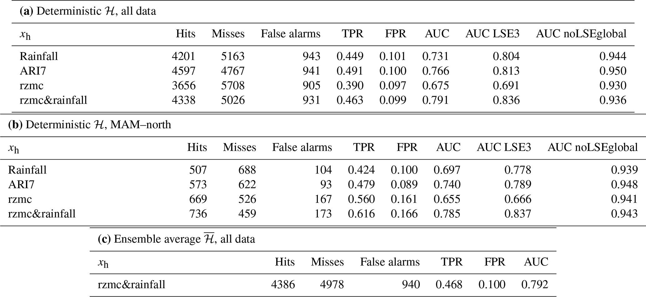
When using the maximum hazard in a 3 d window around the reported LSE (LSE3) and noLSE, performance in terms of AUC strongly increases for rainfall (and ARI7) so that they become similarly well-performing (see Table 2a–b). For rzmc performance is less impacted, and hazard simulations based on rzmc&rainfall are moderately improved. The order of best to worst performing predictor variable(s) remains the same. In contrast, the order is changed when noLSEs are sampled globally without restriction to LSE grid cells (noLSEglobal). For LSE–noLSEglobal, simulations based on ARI7 perform best, followed by those based on rainfall, rzmc&rainfall and finally rzmc. For all four, the AUC values are however really high (>0.93).

To summarize, PHELS ℋ estimates are best in the (wet) winter in the north, and based on LSE–noLSE PHELS performs best when using both rzmc&rainfall as predictor variables. For the analysis of subsequent ensemble results, we therefore focus on this model, unless noted otherwise.

3.2 Ensemble hazard estimates

Figure 7a shows time series of ℋ_ens obtained by PHELS using ensembles of rzmc, rainfall and LSS. The 100 ensemble members are shown in light grey, with $\stackrel{\mathrm{‾}}{\mathcal{H}}$ on top. The range of ℋ between ensemble members is largest for high $\stackrel{\mathrm{‾}}{\mathcal{H}}$. This translates into large ensemble standard deviations for high $\stackrel{\mathrm{‾}}{\mathcal{H}}$, shown in Fig. 7b. The ensemble standard deviation serves as a measure of simulation uncertainty. We observe a peak in the uncertainty for the first three LSEs that occur at peaks in $\stackrel{\mathrm{‾}}{\mathcal{H}}$. For the two LSEs observed in this grid cell in spring 2015, there is a peak neither in $\stackrel{\mathrm{‾}}{\mathcal{H}}$ nor in the uncertainty.

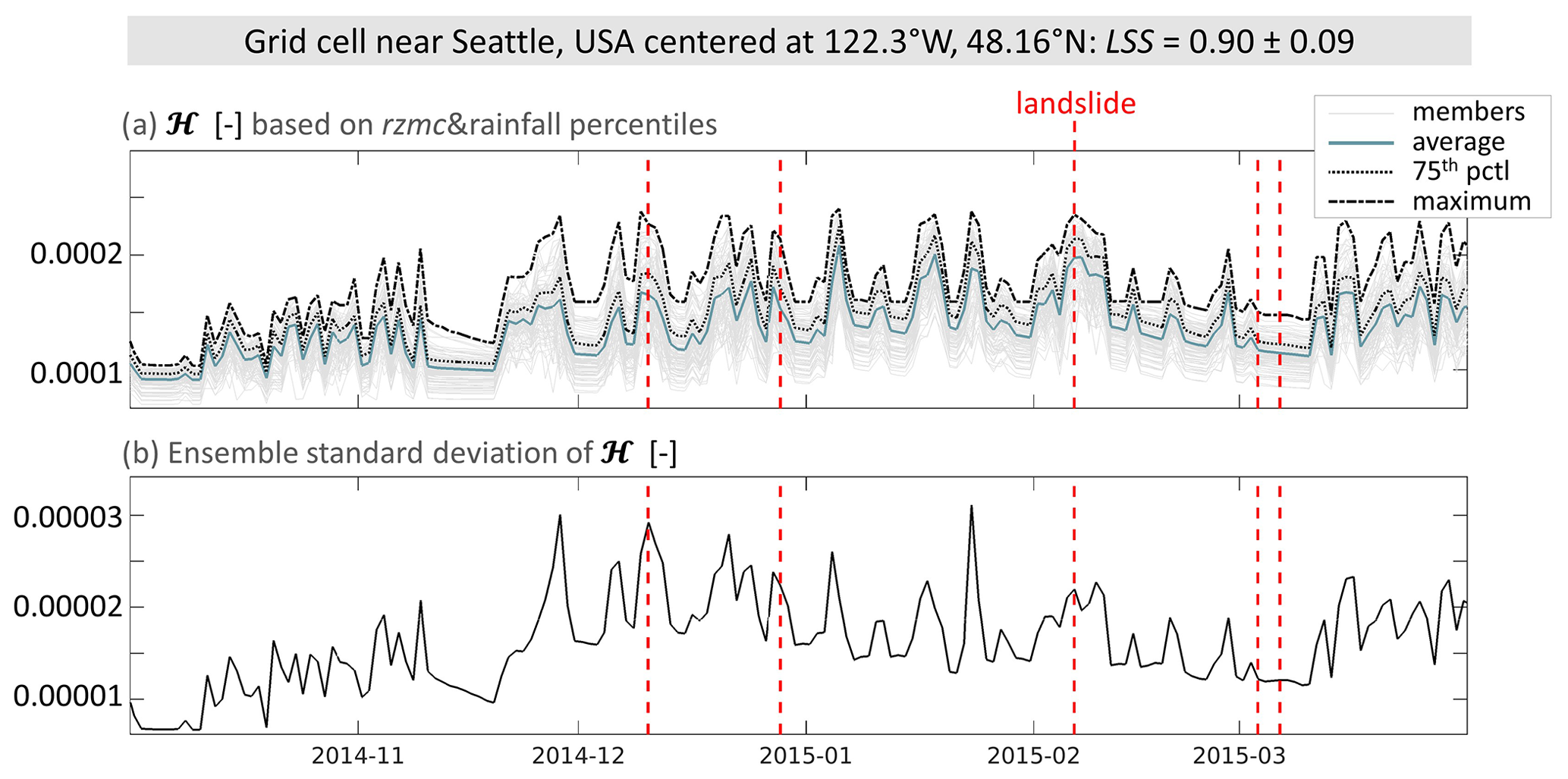
Figure 7 Time series of daily PHELS hazard ensembles (ℋ_ens) based on rzmc&rainfall for a grid cell near Seattle, USA (same as in Fig. 4). (a) Ensemble members as well as ensemble average $\stackrel{\mathrm{‾}}{\mathcal{H}}$, 75th percentile and maximum, (b) ensemble standard deviation. Days with LSE are indicated by the dashed red lines.

Table 2c gives the AUC values for $\stackrel{\mathrm{‾}}{\mathcal{H}}$, as well as the hits, misses and false alarms. Compared to deterministic PHELS for the same hydrological predictor variables, we observe a very minor increase in performance.

To understand the spatio-temporal behaviour of PHELS simulations, Fig. 8 shows spatial distributions of PHELS input data (ensemble average rzmc, rainfall and LSS) and the resulting $\stackrel{\mathrm{‾}}{\mathcal{H}}$ for 15 September 2015. We find elevated $\stackrel{\mathrm{‾}}{\mathcal{H}}$ in Central America, western sub-Saharan Africa, central India and China. These hotspots are located where high values of all three input variables coincide. Note that ℋ uses percentiles of rzmc and rainfall, but that Fig. 8a and b show absolute rzmc and rainfall values, not percentiles. Large rzmc values do therefore not necessarily indicate extremely wet conditions for a specific location. Example of this are the northern hemispheric peat areas in central Siberia or close to the Hudson Bay, which are generally wetter than other regions but are not necessarily wetter than normal on the shown date.

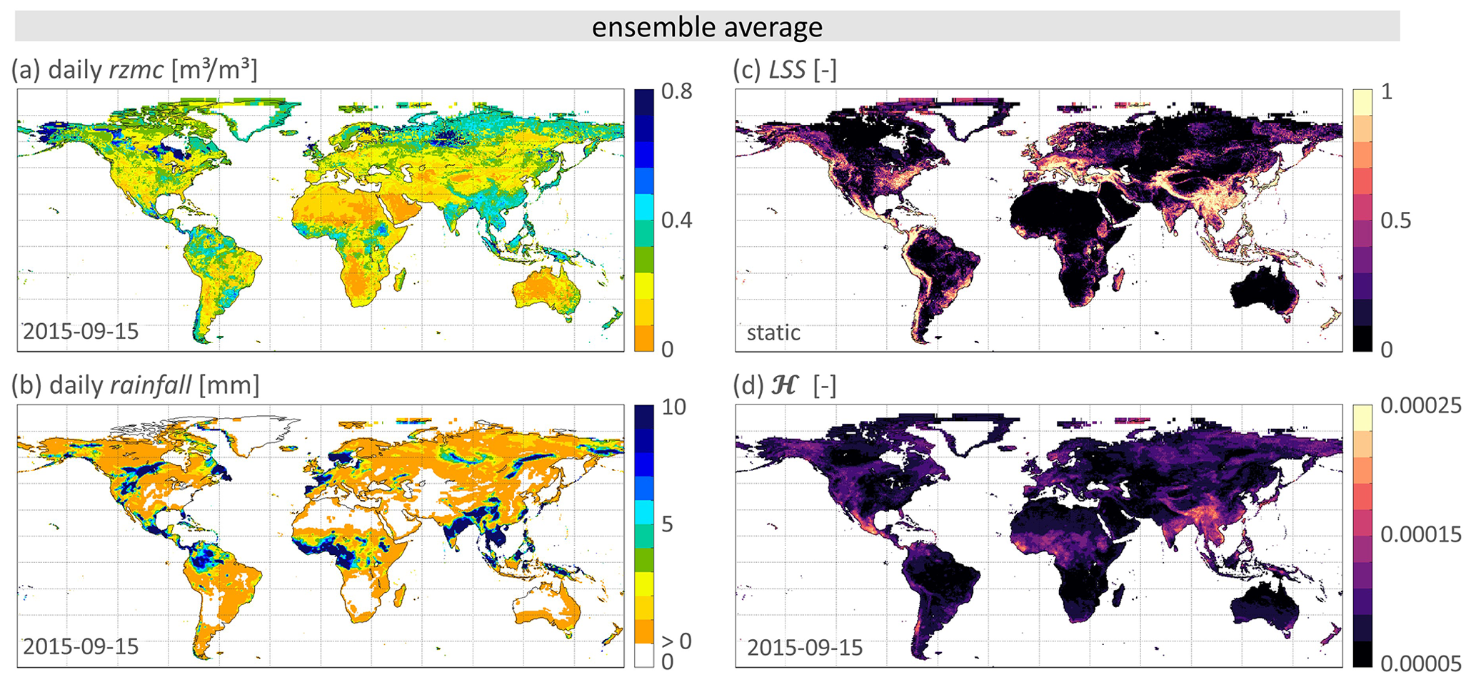
Figure 8 Spatial distribution of PHELS input and output for 15 September 2015. Shown are the grid cell’s ensemble average (a) rzmc [m³ m⁻³], (b) rainfall [mm], (c) static LSS [−] and (d) hazard ℋ [−].

The ensemble standard deviations of PHELS input and output are shown in Fig. 9 for the same day. As for the ensemble averages, we find a high (low) ensemble standard deviation of ℋ, i.e. uncertainty, where high (low) uncertainties of the input variables coincide. Example areas with high uncertainty are Central America and China. Example areas with low uncertainty are the central USA, the Amazon and the Congo basin.

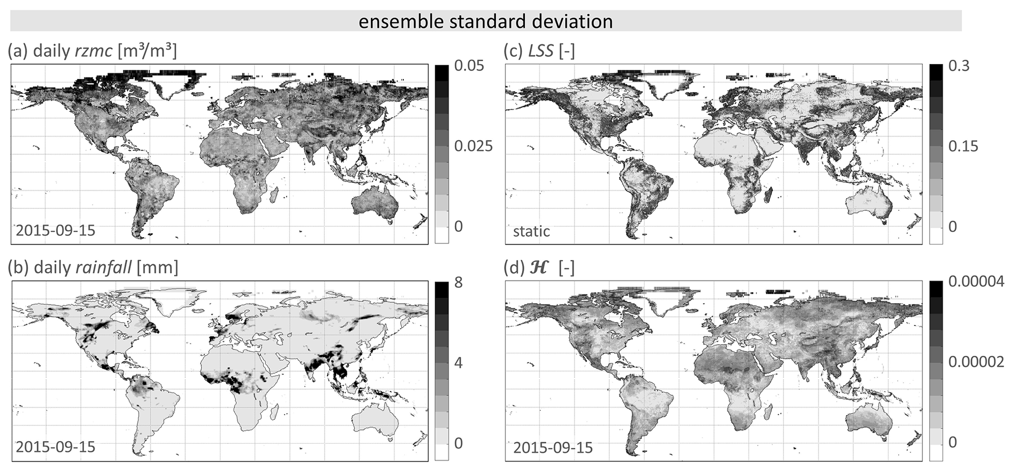
Figure 9 Spatial distribution of PHELS input and output for 15 September 2015. Shown are the grid cell’s ensemble standard deviations of (a) rzmc [m³ m⁻³], (b) rainfall [mm], (c) static LSS [−] and (d) hazard ℋ [−].

The relationship between $\stackrel{\mathrm{‾}}{\mathcal{H}}$ and its uncertainty in terms of standard deviation is illustrated in Fig. 10a for all land grid cells on 15 September 2015. A parabolic pattern between low and high $\stackrel{\mathrm{‾}}{\mathcal{H}}$ values is found, where uncertainty is low at either end and increased in the middle. Furthermore, a more linear trend (“tail”) is found where uncertainty increases proportionally to $\stackrel{\mathrm{‾}}{\mathcal{H}}$. Figure 10b shows $\stackrel{\mathrm{‾}}{\mathcal{H}}$ and standard deviation of ℋ_ens for all LSE and noLSE. Symbols and colour indicate whether LSE and noLSE were correctly captured (true positive – TP; true negative – TN) or not (false positive – FP; false negative – FN), again using the temporal 90th percentile of $\stackrel{\mathrm{‾}}{\mathcal{H}}$ as threshold. The distributions of $\stackrel{\mathrm{‾}}{\mathcal{H}}$ for the positives (TP, FP) are significantly different from that of the TN and they have a peaked distribution. Whereas the distribution for the FN is wider and largely overlaps with the distributions for the positives and the TN. While median uncertainty for FN, i.e. missed alarms, is larger than that for TN, median uncertainty for FP, i.e. false alarm, is nearly identical to that of TP. High uncertainty is therefore not necessarily an indicator of a wrong prediction. Overall, across all time steps and all grid cells globally, the uncertainty is between 5.2 $\times {\mathrm{10}}^{-\mathrm{6}}$ % and 37.5 % of the estimated hazard value, with an average of 13.6 %.

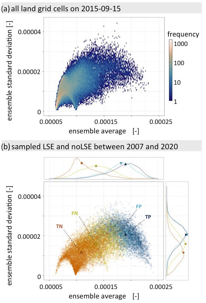
Figure 10 Bivariate histogram of ensemble average $\stackrel{\mathrm{‾}}{\mathcal{H}}$ against ensemble standard deviation (a) for all grid cells on 15 September 2015 and (b) for LSE and noLSE during the complete study time period. Colours and shapes indicate whether the predictions are correct (true negative: TN, true positive: TP) or not (false negative: FN, false positive, FP). The marginal distributions of the ensemble average and standard deviation are shown on the top and side panels. Median values are indicated by the larger symbols on top of the scatter cloud and on the marginal distributions. As a threshold for $\stackrel{\mathrm{‾}}{\mathcal{H}}$ predictions to count as LSE or noLSE, we use the 90th percentile of ℋ per grid cell.

4 Discussion

We evaluate PHELS against the set of LSE that was also used to derive optimal parameter values for Eqs. (5)–(6), which describe the signature relationships (Vrugt and Sadegh, 2013) between predictor variables and ℋ. This fit was hence based on a long-term and spatially aggregated frequency distribution of LSE and not on individual LSE conditions, and has the advantage of robustness because a maximum amount of data was used. In the subsequent evaluation, the match between individual simulated and reported LSE and noLSE is measured in terms of e.g. AUC values, and this focuses on different aspects than the fit on a summary distribution of LSE. A similar procedure has been followed by Calvello and Pecoraro (2019) and Guzzetti et al. (2007) to obtain and evaluate their probabilistic respectively intensity–duration thresholds. Other options could have been to separate the LSE data into a training and a test subset as was done by Stanley et al. (2021), but this would reduce the number of data points both for fitting and validation.

PHELS performance increased when accounting for possible errors in the dating of LSE as well as time zone shifts (LSE3), i.e. PHELS often simulates hazard peaks within 3 d windows around LSE, regardless of the predictor variable(s). This is in line with findings of Kirschbaum and Stanley (2018). For LSE3, ℋ performance based on rainfall approaches that of ARI7, because offsets between the timing of short-term rainfall and LSE are less penalized. The ℋ performance based on rzmc is least impacted by the extended time window, because rzmc is typically slowly varying in time (seasonal). For this assessment, noLSE were only sampled within grid cells of reported LSE to emphasize the temporal aspect in the evaluation. When sampling noLSE globally randomly (noLSEglobal), we find very good ℋ performance for all predictor variables, i.e. global spatio-temporal patterns of hazard are equally well captured, reinforcing the quality of the (LSS) estimates by Felsberg et al. (2022b).

As hydrological predictor variables we investigated daily rainfall, ARI7 from MERRA-2 and rzmc from CLSM. Other datasets could be used (e.g. rzmc estimates from satellite-based data assimilation, as in Felsberg et al., 2021; Stanley et al., 2021), the predictors could be preprocessed differently, e.g. into daily or 3-hourly rainfall maximum (Patton et al., 2023), monthly rainfall (Luna and Korup, 2022), antecedent soil moisture (Mirus et al., 2018), soil moisture changes (Wicki et al., 2020), or short- and long-term anomaly values. Furthermore different combinations of the predictors could be tested, e.g. rzmc and ARI7. Percentile thresholds could moreover be derived for shorter time periods (seasonal, pentad), allowing for intra-seasonal hazard estimations. Note that if the connection of any of these predictor variables with LSE would differ from the exponential behaviour found for all predictor variables used in this study, the form of the fitted Eqs. (5)–(6) would need to be adapted. Furthermore, when multiple time-varying hydrological predictors are used, it could be recommended to implement the normalization factor in Eq. (3): given the use of percentile values for the time-varying predictors, the probability for a single predictor variable is uniform (and normalization would not alter the results), but the joint probability of multiple percentile predictors is not uniform (and would alter the temporal behaviour of PHELS).

PHELS can combine any hydrological variables or even other triggering sources (e.g. seismic). Inclusion of a third predictor variable changed ℋ output characteristics from exponential to quasi-normal (see Appendix A), which allowed the use of a simple ensemble standard deviation as a metric for the ℋ uncertainty. Any further or renewed extension requires a check of distribution characteristics and the statistical measures to quantify uncertainty should be chosen accordingly.

The ℋ_ens uncertainty in terms of ensemble standard deviation follows a parabolic pattern and a linear upward trend with increasing $\stackrel{\mathrm{‾}}{\mathcal{H}}$. The first is induced by the characteristics of rzmc and LSS, which also show parabolic relationship between ensemble average and standard deviation (Felsberg et al., 2022b). The second reflects the behaviour of rainfall and its standard deviation. However, the uncertainty decreases again for very large $\stackrel{\mathrm{‾}}{\mathcal{H}}$ which is likely a result of the design and boundedness of the input variables x_h (percentiles). The sampling (and resampling) of the predictor variable values at the lower (upper) edge of the definition range, i.e. at percentile 1 (percentile 100), will inevitably lead to smaller ensemble standard deviations.

This connection of ℋ_ens uncertainty with the uncertainty of the input variables generates a spatial pattern that is closely following the input patterns. As examples for low ℋ_ens uncertainty on 15 September 2015 we found central USA, the Amazon and the Congo basin (see Fig. 8). These regions have low LSS, and they exhibit dry conditions at this time (low rzmc and low or no rainfall) with small connected uncertainty: consequently, low $\stackrel{\mathrm{‾}}{\mathcal{H}}$ values and ℋ_ens uncertainties are found. Since these regions have nearly no observed LSE (see Fig. 1), sampled grid cells would probably be true negatives (TNs). For the complete study period TN also showed lowest $\stackrel{\mathrm{‾}}{\mathcal{H}}$ and ℋ_ens uncertainty (see Fig. 10b). As examples for high ℋ_ens uncertainty on 15 September 2015 we found Central America and China. Both record a large number of observed LSE and high LSS with low uncertainty. However, rzmc is intermediately high with increased uncertainty and rainfall is high with large uncertainty, resulting in ℋ_ens uncertainty also being high. Sampled grid cells would probably be positive predictions (TP, FP), which for the complete study period also showed highest $\stackrel{\mathrm{‾}}{\mathcal{H}}$ and ℋ_ens uncertainty (see Fig. 10b).

The spatial resolution in this study (36 km) is much coarser than a typical landslide extent. This helps to improve (not degrade) the hazard estimates, because it is easier to estimate the chance for a landslide in a large pixel than at a specific location (scaling effect). The 36 km simulated ℋ thus describes spatio-temporal patterns of landslide probability for a larger area rather than for a single slope. Similar to LSS, spatial variation of ℋ within one grid cell extent can be expected where the environment is very heterogeneous, and this will be partly captured in the ℋ_ens uncertainty. The temporal evolution of ℋ, on the other hand, is governed by hydrology and meso-scale meteorology, which are attributed with autocorrelation lengths of up to 40 km even in strongly mountainous terrain such as the Swiss Alps (Mittelbach and Seneviratne, 2012). A 36 km grid cell time series will thus adequately represent the temporal ℋ variability.

The comparison of hydrological predictor variables shows that PHELS based on ARI7 or rainfall performs best when rainfall is above average (above 50th percentile, not shown), and PHELS based on rzmc performs best when rzmc is above average. As a compromise, the hydrometeorological approach using rzmc&rainfall performs slightly worse than rzmc (or rainfall) alone for elevated rzmc (rainfall) but much better for conditions of dry soil (no rainfall). This is also visible in the stratified AUC analysis, where AUC values range much closer together for rzmc&rainfall. Including rzmc on top of rainfall as a predictor variable specifically improves the performance in spring when other water sources (e.g. meltwater) may be present. We found that including rzmc reduced missed alarms (on wet soils even small rainfall events may induce an LSE) and false alarms (where the soil is dry, LSE occurrence is less likely) for the full data set. The reduction in false alarms was also reported by Ponziani et al. (2012); Mirus et al. (2018); Segoni et al. (2018a); Stanley et al. (2021). While the number of missed alarms is lower for PHELS based on rainfall&rzmc than for PHELS based on rainfall alone, it is even lower for PHELS based on ARI7. A possible reason for this can be that (intensive) antecedent rainfall prepares failure by progressively destabilizing the slope.

PHELS can be compared to different versions of LHASA (Kirschbaum and Stanley, 2018; Stanley et al., 2021) while keeping in mind the large discrepancy in spatial resolution (36 km vs. 1 km), the ratio of LSE to noLSE sampling (1:1 vs. roughly 1:10 000), the method of LSE and noLSE sampling (see LSE3, noLSEglobal), and the thresholds in probabilistic ℋ where applicable. The following skill values for PHELS and LHASA refer to an evaluation of the hazard on the reported day of LSE. The first setup of LHASA combined ARI7 and LSS into categorical “nowcasts” (Kirschbaum and Stanley, 2018) and is comparable to PHELS using ARI7 as hydrological predictor variable. The latter yields a TPR of 0.49, which is above the range of reported TPR for LHASA (0.13 for an earlier version of GLC, 0.23 for LRC, and 0.38–0.45 with additional large-scale rainfall event inventories) (Stanley et al., 2021). LHASA version 2.0 has a different setup (probabilistic combination of different input variables, among these slope, rainfall, soil moisture; see Stanley et al., 2021), which is comparable to PHELS based on rzmc&rainfall. For the latter, we find a TPR of 0.46, whereas Stanley et al. (2021) find TPR values of 0.17 (GLC, also used as training data), 0.32 (LRC, test data) and up to 0.93 with additional inventories. For PHELS, using the 90th temporal percentile within a grid cell as a threshold results in 10 % positive predictions. Because landslides are rare events, the FPR also ranges close to this (0.1) but may differ for temporal subsets (see Table 2). Due to the choice in threshold and the larger LSE–noLSE sampling ratio (see above), this FPR is by design much higher than those for LHASA predictions (between 0.002 and 0.01, Kirschbaum and Stanley (2018); Stanley et al. (2021)). For both models, FPR might however be erroneously high due to known underreporting in the GLC, even within well-reported areas. Figure 4 for example misses mid–late January events of 2016 in the Seattle area that were reported by Mirus et al. (2018).

This known incompleteness of the inventory not only influences the performance evaluation, but also adds to the uncertainty of the model fitting process (i.e. Eqs. 5–6). While the goodness of fit can be quantified (see Table 1) and theoretically propagated, it is still relative to the available inventory. Quantification of inventory-induced uncertainty requires very detailed or synthetic landslide inventories and has been subject of many studies for LSS (Steger et al., 2017; Lin et al., 2021) but less so for hazard assessment. PHELS does not account for such inventory-induced uncertainty, but it does include the uncertainties and within-grid-cell heterogeneity of input variables by using an ensemble approach. The latter allows one to easily account for, for example, the uncertainty in rainfall, which is directly available from ensemble weather prediction systems. Or to account for modelled soil moisture uncertainties, which can be obtained from ensemble land surface model simulations that are usually optimized to match to the variations in observations. Nevertheless, models are always a simplification of real-world conditions, and the downscaling of coarse-scale model estimates to fine-scale applications remains a challenge.

PHELS provides reliable insights into spatio-temporal patterns of landslide hazard but has limitations in the context of actual early warning systems. These usually require higher spatial resolution and temporal accuracy. The coarse spatial resolution would hence call for downscaling methods to obtain within grid-box distributions. And although we use the evaluation approach LSE3 because of time shifts and possible observation errors, the fact that peaks of hazard are often simulated within a 3 d window around a recorded LSE may also indicate a low temporal accuracy, which might be mainly associated with the coarse-scale global re-analysis input of precipitation. For early warning systems the question moreover remains how to interpret or use the hazard uncertainty. Low-enough uncertainty could be used as a secondary condition before warnings are issued to the public or the uncertainty could be directly communicated as is. However, ensemble measures such as the maximum predicted hazard (“worst-case scenario”) or the 90th quantile of ensemble hazard prediction might be easier to understand. While this study used PHELS with specific spatio-temporal resolution and input data, its adjustable, modular character makes PHELS a general framework for hazard estimation that can be tailored to specific purposes. If adequate landslide and hydrological data are available, it would therefore be possible to create a PHELS setup that is more suitable for local to regional landslide early warning systems.

5 Conclusions

In this study, we created the global Probabilistic Hydrological Estimation of LandSlides (PHELS) model, which produces daily landslide hazard [−] (ℋ) estimates at a coarse 36 km resolution. The PHELS model combines landslide susceptibility (LSS) and (percentiles of) hydrological predictor variables such as rainfall, a 7 d antecedent rainfall index (ARI7) or root-zone soil moisture content (rzmc). Apart from deterministic ℋ simulations, PHELS supports landslide hazard ensemble (ℋ_ens) simulations based on repeated sampling of LSS and the hydrological predictor variables. The resulting spread among the ensemble members is a measure of the uncertainty of the simulations. To our knowledge, this is the first global landslide hazard model with uncertainty quantification. We conclude the following:

1. Deterministic ℋ estimates with PHELS yield area under the ROC curve (AUC) values above 0.68, with the best performance (AUC = 0.79) based on the combination of rainfall and rzmc as hydrological predictor variables and second best based on ARI7 (AUC = 0.77). Including rzmc on top of rainfall can reduce missed alarms (especially during spring) and false alarms. The performance of ensemble average ℋ ($\stackrel{\mathrm{‾}}{\mathcal{H}}$) is similar.

2. ℋ_ens uncertainty follows the behaviour of the input variable uncertainties (rainfall, rzmc and LSS) and is about 13.6 % of the daily simulated $\stackrel{\mathrm{‾}}{\mathcal{H}}$ value globally and for the study period. The uncertainty follows a parabolic pattern introduced by the characteristics of rzmc and LSS where rainfall uncertainty is small and a positive linear relationship where rainfall uncertainty is large. Overall, the uncertainty of ℋ simulations is small for very low and very high ensemble average ℋ and larger for intermediate values.

The PHELS model is a flexible framework that allows the inclusion of other hydrological predictors or data sources (satellite data products, data assimilation) in future research. The approach can also be promising at smaller scales with local (in situ) data or for seasonal modelling and offers a scaleable way to propagate uncertainties of various contributing predictors to traceable ℋ uncertainty estimates.

Appendix A: Distribution comparison

In addition to the ROC analysis, we evaluate the performance of deterministic PHELS for all hydrological predictor variables (rzmc, rainfall, ARI7 and rzmc&rainfall) in terms of ℋ distributions for LSE and noLSE. Specifically, we calculate the area between the quantile–quantile (Q–Q) line and the bisector (A_QQ) normalized by the total area underlying the bisector, as described in Felsberg et al. (2021). The larger A_QQ, the more different the two distributions. A large difference between the distributions implies that the variable in question is able to distinguish well between LSE and noLSE conditions, as discussed in Felsberg et al. (2021). To better highlight the long-term capability of PHELS, we also analyse ℋ relative to the temporal average within a grid cell:

$$\begin{array}{}\text{(A1)}& {\mathcal{H}}_{\mathrm{rel}}={\displaystyle \frac{\mathcal{H}-{\mathrm{avg}}_{\mathrm{t}}\left(\mathcal{H}\right)}{{max}_{\mathrm{t}}\left(\mathcal{H}\right)-{min}_{\mathrm{t}}\left(\mathcal{H}\right)}},\end{array}$$

where avg_t, min_t and max_t denote the temporal average, minimum and maximum for this grid cell across the complete time period. For an assessment of the short-term capability, time steps are limited to ±15 d (around the LSE or noLSE in question) across all years to obtain an average, minimum and maximum ℋ within this time window. This relative ℋ is referred to as ℋ_rel,15.

Table A1 Differences between LSE and noLSE distributions of hazard values for PHELS based on different hydrological variables (rainfall, ARI7, rzmc, rzmc&rainfall) measured in terms of normalized A_qq. The corresponding distributions are shown in Fig. A1. Results are shown for the deterministic ℋ, ℋ relative to the temporal range within a grid cell (ℋ_rel) and relative to the long-term average hazard for ±15 d (ℋ_rel,15).

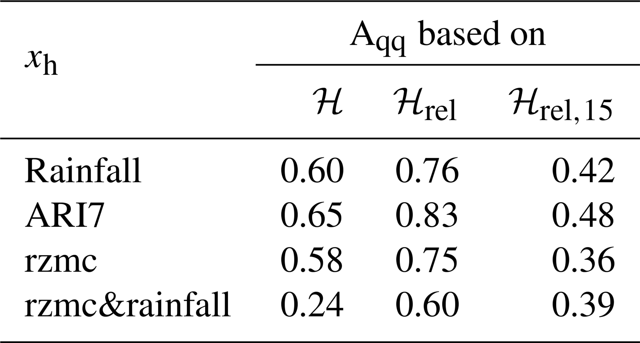
Extracting ℋ for LSE and noLSE results in distributions as displayed in Fig. A1. It illustrates that the inclusion of a second hydrological predictor variable changes results from exponential distributions to quasi-normal distributions. While differences between the distributions of LSE and noLSE can be captured by A_QQ, it is difficult to compare A_QQ across such different types of distributions. Table A1 summarizes A_QQ of all predictor variables for ℋ, ℋ_rel and ℋ_rel,15. ARI7 shows highest A_QQ, i.e. discrimination ability, for ℋ predictions based on one hydrological predictor variable, and rzmc has lowest A_QQ. A_QQ is generally higher (lower) for ℋ_rel (ℋ_rel,15) than for ℋ. For PHELS based on rzmc&rainfall, A_QQ is smaller than for single variable PHELS. At the same time, A_QQ increases for both ℋ_rel and ℋ_rel,15, indicating improvements in the discrimination abilities both for long- and short-term patterns.

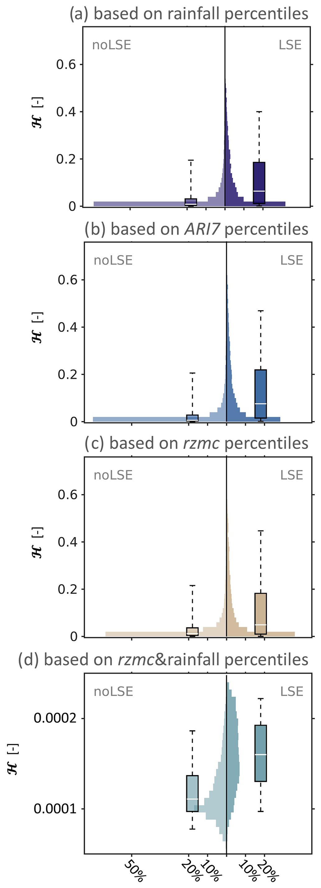
Figure A1 Distribution of PHELS ℋ for known LSE (right, dark value) and sampled noLSE (left, light colour), shown in histograms (background) and boxplots (foreground). Distributions are shown for PHELS based on (a) rainfall percentiles, (b) ARI7 percentiles, (c) rzmc percentiles (x_h in Eq. 5) and (d) rzmc&rainfall percentiles (x_h1 and x_h2 in Eq. 6).

Appendix B: Abbreviations

A_QQ: area between the quantile–quantile (Q–Q) line and the bisector ARI: antecedent rainfall index ARI7: 7 d antecedent rainfall index [mm] AUC: area under the ROC curve CLSM: Catchment Land Surface Model DJF: December–January–February EASEv2: Equal-Area Scalable Earth version 2 FPR: false positive rate GLC: Global Landslide Catalog ℋ: landslide hazard [−] ℋ_ens: landslide hazard ensemble $\stackrel{\mathrm{‾}}{\mathcal{H}}$: ensemble average ℋ JJA: June–July–August LHASA: Landslide Hazard Assessment for Situational Awareness LRC: Landslide Reporter Catalog LSE: landslide event LSS: landslide susceptibility MAM: March–April–May MERRA-2: Modern-Era Retrospective analysis for Research and Applications, Version 2 noLSE: no landslide event PHELS: Probabilistic Hydrological Estimation of LandSlides rzmc: root-zone soil moisture content [m³ m⁻³] ROC: receiver operation characteristic SON: September–October–November TPR: true positive rate