Future heat extremes and impacts in a convection-permitting climate ensemble over Germany

Heat extremes and associated impacts are considered the most pressing issue for German regional governments with respect to climate adaptation. We explore the potential of a unique high-resolution, convection-permitting (2.8 m), multi-GCM (global climate model) ensemble with COSMO-CLM (Consortium for Small-scale Modeling Climate Limited-area Modelling) regional simulations (1971–2100) over Germany regarding heat extremes and related impacts. We find a systematically reduced cold bias especially in summer in the convection-permitting simulations compared to the driving simulations with a grid size of 7 km and parametrized convection. The projected increase in temperature and its variance favors the development of longer and hotter heat waves, especially in late summer and early autumn. In a 2 ^∘C (3 ^∘C) warmer world, a 26 % (100 %) increase in the heat wave magnitude index is anticipated. Human heat stress (universal thermal climate index (UTCI) > 32 ^∘C) and region-specific parameters tailored to climate adaptation revealed a dependency on the major landscapes, resulting in significantly higher heat exposure in flat regions such as the Rhine Valley, accompanied by the strongest absolute increase. A nonlinear, exponential increase is anticipated for parameters characterizing strong heat stress (UTCI > 32 ^∘C, tropical nights, very hot days). Providing region-specific and tailored climate information, we demonstrate the potential of convection-permitting simulations to facilitate improved impact studies and narrow the gap between climate modeling and stakeholder requirements for climate adaptation.

1 Introduction

The last 2 decades have been characterized by an increased number of summer heat waves (HWs), some of them of unprecedented magnitude and impact (e.g., Schär and Jendritzky, 2004; García-Herrera et al., 2010; Barriopedro et al., 2011; Russo et al., 2015). HWs are the most visible sign of ongoing global warming in central Europe (IPCC, 2023), which lead to an increased awareness in our society and stakeholders (Lee et al., 2015; Moser, 2016). As a result, both government agencies and the private sector have developed plans not only for long-term investments towards climate protection but also for the development of sustainable adaptation strategies, which are now regularly finding their way into policy agendas (Biesbroek et al., 2010). In Germany, local governments are key actors implementing adaptation strategies (Hackenbruch et al., 2016). Nearly one-fourth of the German cities had climate adaptation plans in place by 2018 (Reckien et al., 2018), documenting an increasing interest in the subject. Moreover, the German federal government has launched large research activities like the RegIKlim consortium (regional information for action on climate change) to further strengthen this development.

From the perspective of administrations in municipalities in southern Germany, the greatest need for action lies indeed in adapting to heat extremes (Hackenbruch et al., 2017). HWs – increased temperature over several consecutive days – are a threat to ecosystems, the economy, and human health (e.g., Basu and Samet, 2002; Poumadere et al., 2005). HWs are in fact the weather hazard causing the highest number of deaths in Europe (Zuo et al., 2015); e.g., for the European HW in 2003 alone, up to 80 000 additional deaths were recorded in over 12 European countries concerned by excess mortality (Robine et al., 2007). However, there is no unified definition of a HW. Different thresholds for, e.g., length and temperature can be found in the literature, and a variety of indices have been developed for classification, e.g., warm spell duration index (WSDI) (Alexander et al., 2006), heat wave magnitude index (HWMId) (Russo et al., 2014), or excess heat factor (EHF) (Nairn and Fawcett, 2015). Recent efforts have gone towards quantitative approaches and a higher comparability between methods (e.g., Perkins and Alexander, 2013; Russo et al., 2014; Becker et al., 2022), leading to a better understanding of the strengths, weaknesses, and range of applicability of the individual indices. Irrespective of the index used, there is a clear consensus in the scientific community (IPCC, 2023) that HWs will become more severe in terms of duration, frequency, and magnitude with increasing global warming, also in central Europe.

Climate information on the regional to local scale is needed for the development of tailored climate adaptation measures. This can be achieved with regional climate models (RCMs) which perform a downscaling of the climate projections from global climate models (GCMs) to the required spatial scales and timescales, as is done in the Coordinated Regional Downscaling Experiment (CORDEX) (e.g., Jacob et al., 2014). Novel developments include RCM simulations performed with a grid spacing under 4 km, which resolves convection-permitting scales, thus making parametrizations of deep convection not required (convection-permitting models, CPMs) (Prein et al., 2015). Due to the very high resolution on the scale of urban districts, either relevant data fields can be derived directly or a direct coupling with impact models can be allowed. Several recent studies have documented the advantages of these convection-permitting simulations, in terms of both dominant convective precipitation and regions with strong spatial heterogeneity as present in mountainous or urban areas (Prein et al., 2015). Regarding the representation of temperature, there is not yet a consensus on added value in convection-permitting simulations. Whereas Prein et al. (2013) and Brisson et al. (2016) attribute improvements in the temperature output to the better resolution of orography, Ban et al. (2014) even found an increasing bias on the convection-permitting scale but improvements in the diurnal cycle of temperature in a domain covering the alpine region. In contrast, an improvement in mean temperature was found in Hohenegger et al. (2008) for most of the study area and in investigations by Hackenbruch et al. (2016) over Germany. In addition, Tölle et al. (2018) found an added value for temperature extremes. Mixed results with a regional dependency were found in Soares et al. (2022), concluding a gain for temperature due to an improved spatial representation of local atmospheric circulations and land–atmosphere interactions.

To quantify the associated uncertainties of the regional climate projections, ensemble simulations are required. As the computational costs of CPMs are (very) high, many climate studies are based on single-model projections, and only a few studies using CPM ensembles exist (Prein et al., 2015). The very first ensembles of convection-permitting climate projections exist, e.g., from the CORDEX Flagship Pilot Study on Convection (FPSConv; Pichelli et al., 2021; Ban et al., 2021). There, several GCMs from the Coupled Model Intercomparison Project (CMIP5) (Taylor et al., 2012) using the RCP8.5 scenario (Van Vuuren et al., 2011) were downscaled by multiple RCMs to a common grid with 3 km resolution covering the larger Alpine area (ALP-3). They used 10-year time slices for the historical period (1996–2005) and two future periods (2041–2050 and 2090–2099). The current study applies a different ensemble approach, which is a four-member ensemble of convection-permitting climate projections performed by a single RCM, downscaling four GCMs under the scenario RCP8.5. All simulations cover the period from 1971 to 2100 in a quasi-transient manner, where the projection is composed of several time slices. To our best knowledge, an ensemble of this temporal extent is currently unique. Such a long simulation period allows for a better statistical representation of extremes and the application of approaches used for typical coarser-scale transient GCM or RCM ensembles, e.g., the analysis for different global warming levels (GWLs) as is used in the IPCC AR6 (Lee et al., 2021) to compare climate change signals for GCMs with a different climate sensitivity or between different emission scenarios.

Our focus in this study is heat extremes and related impacts under global warming compared to recent climate conditions. Specifically, we were motivated by three guiding questions:

1. What are the benefits of convection-permitting models for temperature extremes in Germany (Sect. 3)?

2. What can we learn from a convection-permitting ensemble about future regional temperature trends and HW characteristics (Sects. 4 and 5)?

3. What is the impact of these changes on heat stress and other regionally mapped tailored climate parameters (Sect. 6)?

The paper is structured as follows: Sect. 2 describes the methodology and the datasets used. Sections 3–6 focus on the results guided by the three research questions, while a summary and discussion conclude the paper in Sect. 7.

Voldoire et al. (2013)Giorgetta et al. (2013)Prodhomme et al. (2016)Collins et al. (2011)

Table 1 Name, realization, equilibrium climate sensitivity (ECS; see the Supplement in Nijsse et al., 2020), 30-year periods corresponding to GWL +2 and +3 ^∘C relative to pre-industrial conditions, and main reference for the CMIP5 GCMs downscaled for the ensemble.

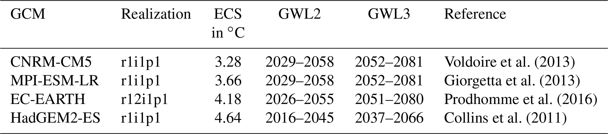
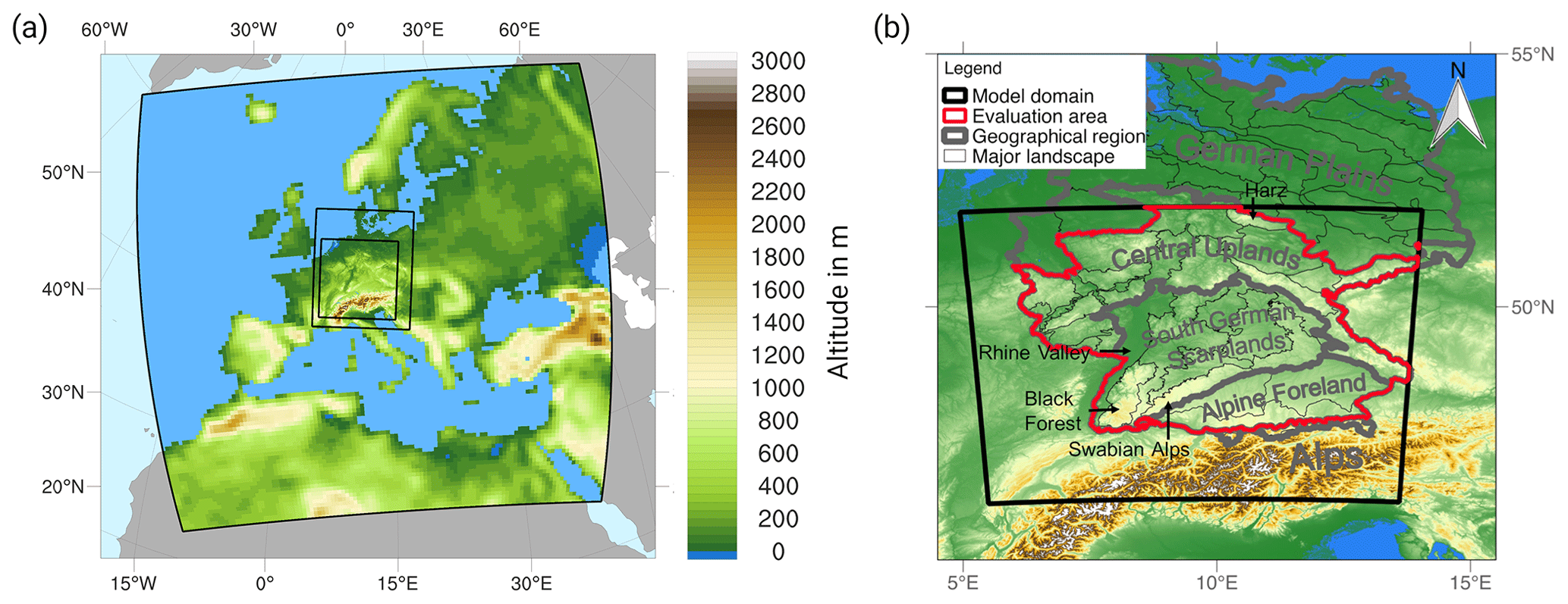
Figure 1 In (a) the three nesting levels are shown. Panel (b) shows the model domain with the sponge area truncated and the evaluation area used in red. The borders of the German major landscapes were added in black. Important major landscapes for the evaluation are the Rhine Valley, the Black Forest, the Swabian Alps, and the Harz (shapefiles of the major landscapes: BfN, 2015).

2 Data and methods

2.1 The COSMO-CLM ensemble

The simulations analyzed in this study have been generated in the context of the project KLIWA (Klimaveränderungen und Konsequenzen für die Wasserwirtschaft) and extended within the project ISAP (integrative urban-regional adaptation strategies in a polycentric growth region: model region Stuttgart). The regional climate simulations are conducted using the RCM COSMO5.0-CLM9 (Consortium for Small-scale Modeling Climate Limited-area Modelling; CCLM; Rockel et al., 2008). CCLM originates from the German weather service forecast model COSMO (Baldauf et al., 2011), which is a three-dimensional, non-hydrostatic, fully compressible numerical model for the atmosphere including a multi-layer soil–vegetation transfer model TERRA-ML (Schrodin and Heise, 2001). The RCM has been applied in multiple studies over different CORDEX domains (Sørland et al., 2021) and on the kilometer scale within the CORDEX Flagship Pilot Study on Convection (Ban et al., 2021; Pichelli et al., 2021).

Initial and boundary data are provided by four GCMs (see Table 1) from the CMIP5 generation under the scenario RCP8.5 (Van Vuuren et al., 2011). The selected GCMs cover a wide range of climate sensitivities (Nijsse et al., 2020) that are parametrized over the equilibrium climate sensitivity (ECS) – the global mean surface air temperature increase that results from a doubling of atmospheric CO₂ (Table 1). In addition, an evaluation simulation was carried out with a downscaling of ERA40 (Uppala et al., 2005) over the period 1971–2000 (Hackenbruch et al., 2016), using the same setup as the projections.

The ensemble was generated in a three-step nesting approach (Table 2; Fig. 1a) with a first nest over Europe with 0.44^∘ grid resolution, an intermediate nest over central Europe with 7 km resolution, and an inner nest that encompasses the area of central and southern Germany and the Alpine area with 2.8 km resolution. The convection for the first two nests is parametrized using the Tiedtke scheme (Tiedtke, 1989). For the innermost domain, this parametrization is only used for shallow convection as in Hackenbruch et al. (2016). In the current setup, the boundary zone between the inner nests is relatively narrow. However, we can benefit from a relatively small horizontal-resolution step (less than a factor of 3) between the nests, which is smaller than common convection-permitting setups used today (Ban et al., 2021). This is likely to decrease boundary effects and enable a tighter nesting. Nevertheless, the boundary zone that was excluded for the analysis of the innermost domain was considerably large (48 grid points, 137 km). Our examination of the results revealed that anomalies of temperature, as well as mean and extreme precipitation, occur well outside the evaluation area. The first two nesting levels were performed in a transient way. The third nest was originally performed in 30-year time slices preceded by a 3-year spin-up (1968–2000, 2018–2050, 2068–2100; Schädler et al., 2018). These time slices were later extended (2001–2020, 2051–2070) to provide a quasi-transient ensemble for the whole period. The overlapping periods (2018–2020 and 2068–2070) were compared (not shown). No relevant differences were found several months after simulation start, in accordance with the findings from Lavin-Gullon et al. (2023).

(Tiedtke, 1989)(Tiedtke, 1989)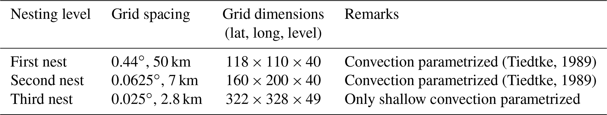

Table 2 Model setup.

This continuous time-series data enabled us to apply the concept of global warming levels (GWLs) (Lee et al., 2021), allowing an improved comparability from the downscaling of GCMs with differing climate sensitivities or different emission scenarios. Therefore, this approach mitigates parts of the GCM and scenario uncertainties and provides more specific information about the effects of climate change given a certain threshold of warming. Specifically, we analyze the +2 and +3 ^∘C GWLs, which was possible for all GCMs due to the use of the high-end scenario RCP8.5. An overview of the simulations is given in Table 1. The period 1971–2000 is used as a historical reference period, which is attributed a global warming of 0.46 ^∘C. Table 1 lists the 30-year periods for the GCMs, which are centered around the respective year of the threshold exceedance similar to Teichmann et al. (2018).

As a strong dependency of the temperature output on the major landscape was detected, the area is narrowed down to a geographically more homogeneous area (Fig. 1b), including the Central Uplands, the South German Scarplands, and the Alpine Foreland. Therefore, the domain focuses on the hilly parts of Germany, excluding the flat regions in northern Germany and the mountainous regions – the Alps – in the very south. This domain, later referred to as the evaluation area, is bordered in red in Fig. 1b and is used in this study when statistics are applied over several grid points. The analysis in the paper is largely focused on HWs and associated impacts in the warm season. Since we observed the largest changes in late summer and early fall, we limit the analysis in this case to the months of May through October. This period is referred to as the summer half year below.

To evaluate the skill of the convection-permitting simulation, a comparison of observation data with the second convection-parametrizing nest and the third convection-permitting nest is performed on the raw, uncorrected model output in Sect. 3. The HYRAS dataset is used as the observation, which is based on station data that are aggregated to a gridded dataset using the REGNIE method of combining a regression model and inverse distance weighting (Rauthe et al., 2013; Razafimaharo et al., 2020). The comparison is conducted for the reference period 1971–2000 for the evaluation run driven by ERA40, as well as for all ensemble members. Simulation data were interpolated on the HYRAS grid with a grid spacing of 5 km. In addition, a height correction of temperature was applied along with the interpolation, assuming a vertical gradient of 0.0065 ^∘C m⁻¹. The correction compensates for the effect of a height-dependent temperature that is favored by the higher resolution of orography. The evaluation of the model skill was conducted prior to the bias correction.

2.2 Bias correction

In order to correct for a systematic error in climate simulations to obtain reliable data for the impact assessment, it is common practice to apply a bias correction (Maraun, 2016). Following the assumption that the model bias remains constant over time for each quantile of the model data, we apply quantile delta mapping according to Cannon et al. (2015). Its application to a modeled variable x_mod,pred at time step t in the prediction period (pred) is based on its non-exceedance probability P_t, which is evaluated over the cumulative distribution function F (Eq. 1). A quantile mapping of the value with the same non-exceedance probability P_t in the historical period (hist) is performed based on observed reference data (obs). To preserve the relative changes between the historical and the prediction period, the climate change signal Δ_m of the corresponding quantile is multiplied to obtain the corrected value y_mod,pred (Eqs. 2 and 3).

$$\begin{array}{}\text{(1)}& {\displaystyle }& {\displaystyle }{P}_t=F_{\mathrm{mod},\mathrm{pred}}\left(x_{\mathrm{mod},\mathrm{pred}}\left(t\right)\right)\text{(2)}& {\displaystyle }& {\displaystyle }{\mathrm{\Delta }}_m\left(t\right)={\displaystyle \frac{x_{\mathrm{mod},\mathrm{pred}}\left(t\right)}{F_{\mathrm{mod},\mathrm{hist}}^{-\mathrm{1}}\left(P_t\right)}}\text{(3)}& {\displaystyle }& {\displaystyle }{y}_{\mathrm{mod},\mathrm{pred}}\left(t\right)=F_{\mathrm{obs},\mathrm{hist}}^{-\mathrm{1}}\left(P_t\right)\cdot {\mathrm{\Delta }}_m\left(t\right)\end{array}$$

A normal distribution was fitted to the distribution of absolute temperature to derive the transfer function. For the correction of precipitation, the empirical approach is used instead, as no added value was found with the distribution-based method using, e.g., a gamma distribution. In addition, a dry-day correction following Ehmele et al. (2022) was applied prior to the correction for precipitation.

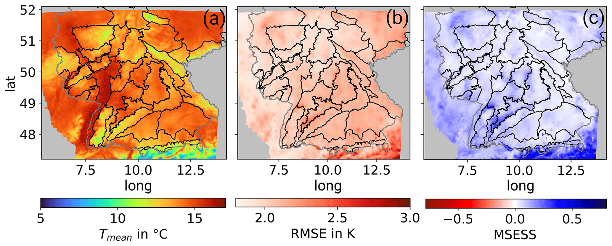
Figure 2 Impact of the bias correction of T_mean in the summer half year (May to October) comparing the ERA40-driven model run with observation. Panel (a) shows the mean summer temperature 1971–2000 in the reference dataset HYRAS, (b) the RMSE of the ERA40-driven model run compared to HYRAS, and (c) the MSESS of the bias-corrected run compared to the uncorrected.

The bias correction was derived for the parameters daily mean temperature T_mean, daily minimum temperature T_min, daily maximum temperature T_max, and the daily precipitation sum P_sum. As reference, the observation dataset HYRAS with a resolution of 5 km was used, which was interpolated to the model grid. Along with the interpolation, a height correction of T_mean, T_min, and T_max was applied assuming a vertical gradient of 0.0065 ^∘C m⁻¹. The available 30 years of the historical time slice from 1971 to 2000 were used as a reference period. To account for seasonal dependencies as discussed in Pierce et al. (2015), evaluation was done over a 3-month window. To minimize discontinuities at the edges of the time window (Pierce et al., 2015), the bias correction was applied for each month i of the year separately, using a transfer function derived and applied over month i−1 to month i+1.

This approach was chosen because it preserves the climate change signal of the quantiles, which is important for the relative description of heat waves used in the study. Furthermore, the method allows an application of the correction in a future climate where the temperature may exceed the range of temperatures in the historical period, which is only possible to a limited extent with classical quantile mapping (Maraun, 2016). However, the underlying assumption and the resulting constant transfer function might not be valid in a future climate (Pierce et al., 2015), leading to potential errors. Furthermore, the use of a parametric approach of fitting an assumed distribution to the data to derive the transfer function is still arbitrarily discussed. Several studies, e.g., Pastén-Zapata et al. (2020) and Qian and Chang (2021), apply a normal distribution for temperature to get a more robust transfer function. Using a fitted function has the additional advantage that the transfer function is independent of any smoothing interval that may be defined (Kerkhoff et al., 2014). On the other hand, parametric approaches introduce additional bias if the distribution of a variable does not accurately match the theoretical distribution. Especially for extreme values, a deviating statistic is assumed according to the extreme value distribution. Quantile approaches, allowing different statistical models for extremes, could potentially reduce uncertainty (e.g., Vrac and Naveau, 2007; Berg et al., 2012; Schubert et al., 2017).

As shown in Fig. 2, major improvements can be achieved by the distribution-based quantile mapping using the example of T_mean. In Fig. 2a the reference data from HYRAS are shown averaged over the summer half year. Comparing these reference data to the simulations driven by ERA40, a root mean square error (RMSE) between 1.95 and 2.18 ^∘C (5th to 95th percentile) is visible in the evaluation area (Fig. 2b). The skill of the applied bias correction is expressed by the mean squared error skill score (MSESS) using the mean square error (MSE; Eq. 4). MSESS is positive all over the domain (Fig. 2c); thus the correction leads to a better alignment of the simulation data with the observation. Stronger improvements coincide with regions of higher deviations of the uncorrected data.

$$\begin{array}{}\text{(4)}& \mathrm{MSESS}=\mathrm{1}-{\displaystyle \frac{{\mathrm{MSE}}_{\mathrm{corr},\mathrm{obs}}}{{\mathrm{MSE}}_{\mathrm{raw},\mathrm{obs}}}}\end{array}$$

2.3 Heat wave and impact indices

Different aspects of heat stress are addressed with this study. We start with the classical approach of describing the meteorological aspects of HWs. Secondly, we will focus on the impact on human health using a thermophysiological description of heat. Finally, climate parameters – threshold-based indices that are tailored to the need of stakeholders in different fields of action – are evaluated. All metrics used are presented in the following.

2.3.1 Heat wave indices

A number of consecutive days with elevated temperature is called a HW. However, a universally fitting definition does not exist, but several definitions can be found in the literature. We use the definition by Russo et al. (2014) heres, in which a HW is defined as an uninterrupted series of at least 3 d where the daily maximum temperature T_max exceeds T_max,90 %, the daily 90th percentile of T_max within a 31 d centered window over the reference period. Several metrics describing different aspects of HWs exist. The length of a HW is derived as the number of consecutive HW days, and its frequency is the average number of HW days per year. As a measure for the HW temperature, we introduce the maximum excess temperature ΔT_max above the 90th percentile threshold. Russo et al. (2014) proposed a heat wave magnitude index (HWMId), an index that can be compared across regions and time, taking HW length as well as temperature into account. The HWMId is calculated as

$$\begin{array}{}\text{(5)}& \mathrm{HWMId}={\displaystyle \frac{T_{\max }-T_{\max ,\mathrm{25}\mathit{\%}}}{T_{\max ,\mathrm{75}\mathit{\%}}-T_{\max ,\mathrm{25}\mathit{\%}}}},\end{array}$$

with T_max,25 % and T_max,75 % the daily 25th and 75th percentile of T_max within a 31 d centered window in the reference period. The event sum over the heat event characterizes the magnitude of a HW.

2.3.2 Human heat stress

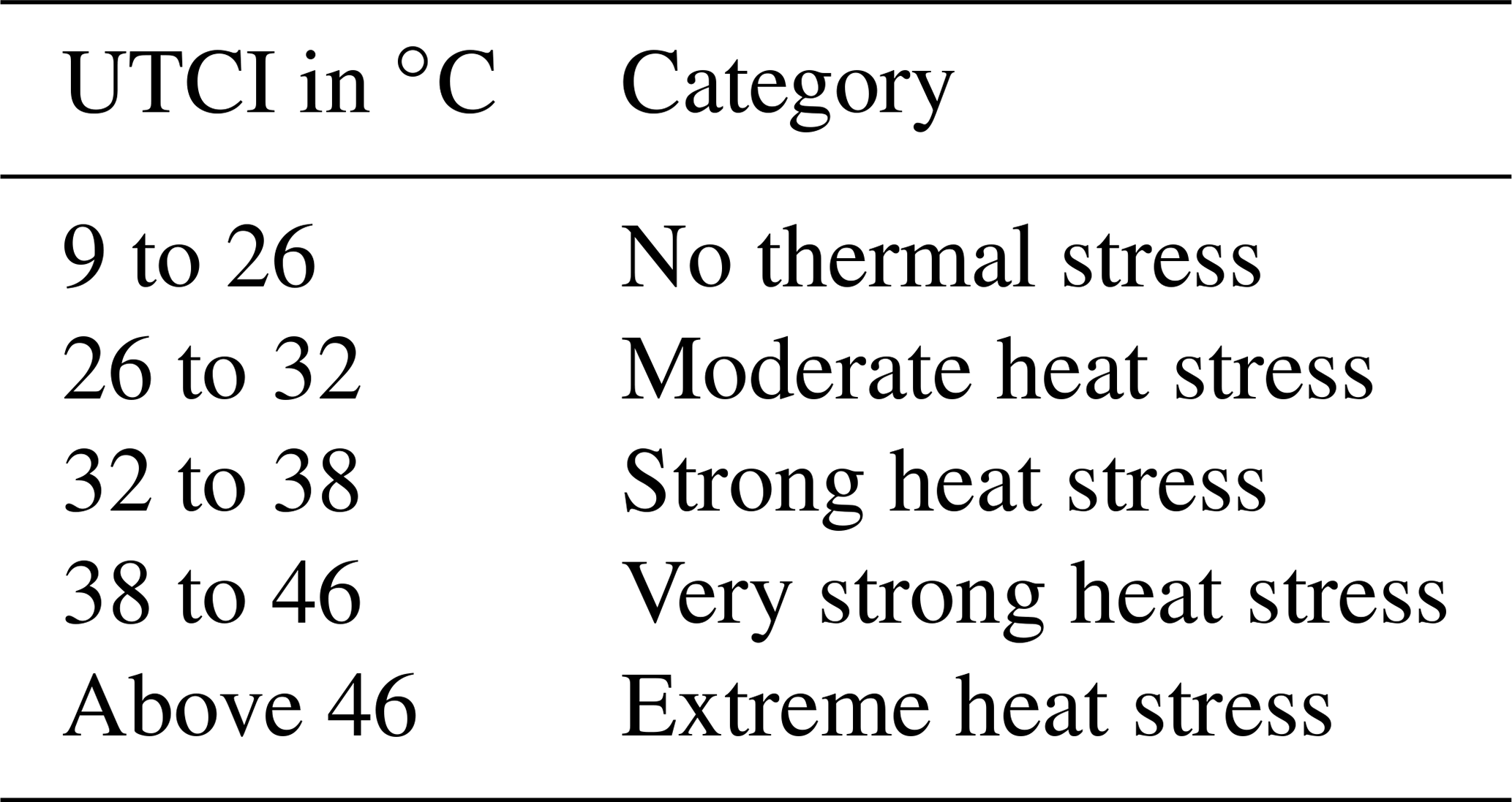
Apart from air temperature, there are additional elements such as clothing, humidity, mean radiant temperature, air movement, and metabolic rate that determine a person's level of thermal comfort (Fanger, 1970). With the requirement to transform this complex system into an application-friendly model, the universal thermal climate index (UTCI) was developed in 2009 from an interdisciplinary collaboration between human thermophysiology, physiological modeling, meteorology, and climatology (Jendritzky et al., 2007). The index is defined as the air temperature of a reference condition causing the same thermal comfort as the actual response. The reference conditions were determined as a wind speed WS=0.5 m s⁻¹ at 10 m height and a mean radiant temperature T_mrt equal to air temperature T_air. The relative humidity in the reference environment is 50 % for temperatures below 29 ^∘C. However, for temperatures above 29 ^∘C, the water vapor pressure is instead kept constant at a level of 20 hPa (Błażejczyk et al., 2013). In Table 3, the defined categories for heat stress are listed. The calculation of the UTCI is based on Fiala's multi-segment model of human physiology and thermal comfort (Fiala et al., 2012), coupled with a clothing model by Havenith et al. (2012). Details can be found in, e.g., Jendritzky et al. (2012), Fiala et al. (2012), and Havenith et al. (2012). The hourly model results were taken as input for the calculation of UTCI in this study. Due to missing hourly gridded observations, no bias correction was applied.

Table 3 Assessment scale of heat stress using the UTCI. Cold stress for UTCI ≤9 ^∘C is not shown here.

2.3.3 User-tailored climate indices

More and more sophisticated indices were developed, focusing on different aspects of heat stress. However, in order to take action in the local governments, the exact information on the change in climatic conditions is not always helpful. The so-called “climate information usability gap” is the barrier of what scientists see as useful and what users consider useful for their decision-making. One key aspect of narrowing the gap is the customization and tailoring of the data to the user's need to improve the usability of climate information (Lemos et al., 2012), often as a co-design approach. In the case of climate adaption strategies, the measures of interest are, according to Hackenbruch et al. (2017), meteorological events leading to an effect on people and health risks (for example, hot days), influence on capital investments or municipal budgets (for example, winter services), or property damage (for example, heavy precipitation events).

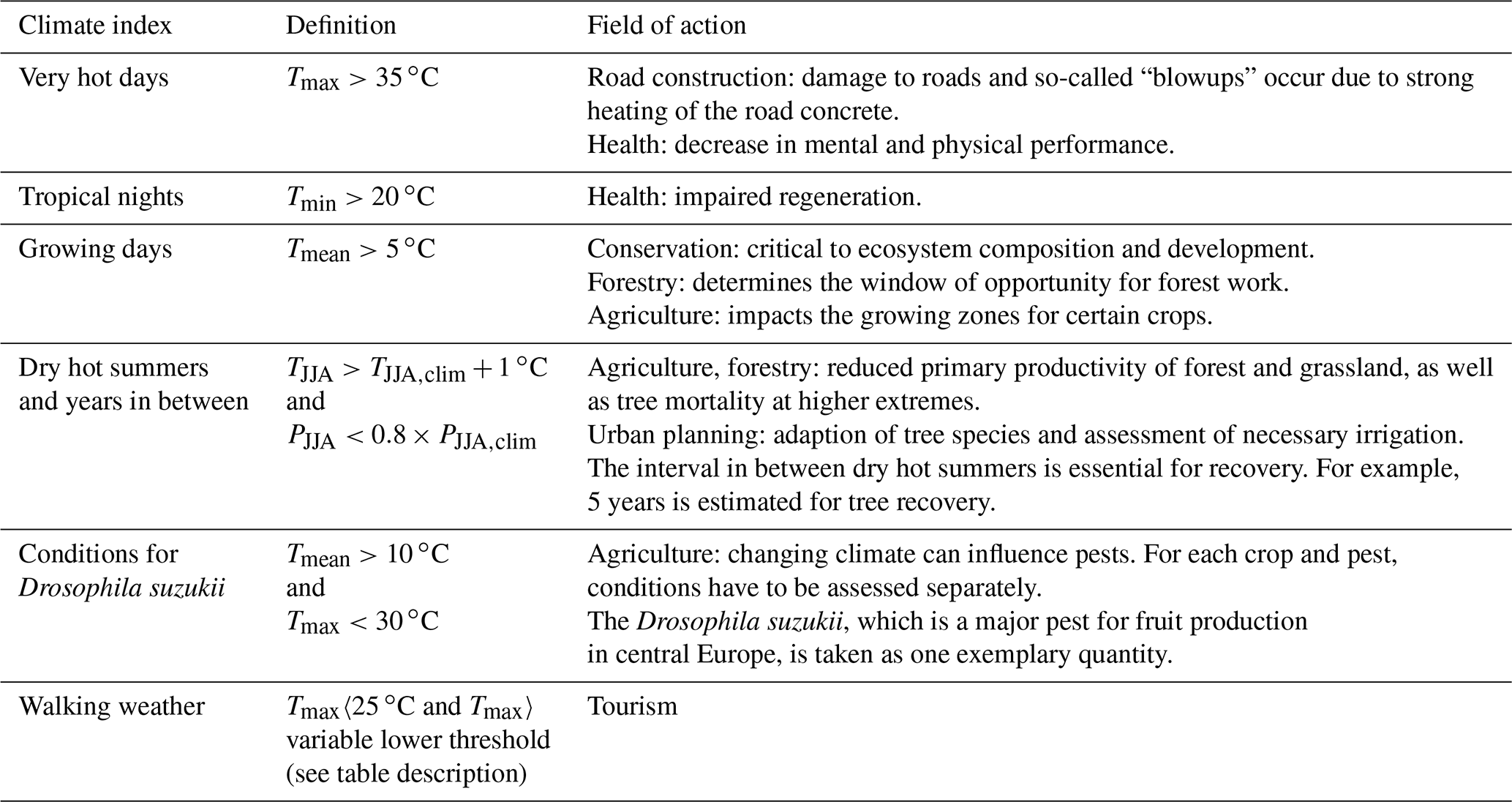
To assess the impact of changing temperature, we present several user-tailored climate parameters following Hackenbruch et al. (2017). The selected parameters, their definition, and field of action are summed up in Table 4. All parameters are related to regional temperature changes but cover different fields of action and therefore are of concern to different stakeholders. The aim of the choice is to show the diversity of the effects of climate change and to present the potential of high-resolution climate models for climate adaptation.

Table 4 Definition and field of action of the tailored climate parameters related to temperature development based on the KLIMOPASS project (Schipper et al., 2016). T is daily mean, max, or min temperature, and T_JJA and P_JJA are the mean daily temperature and precipitation sum from June to August. The subscript “clim” refers to the climatological mean that was calculated over the reference period 1971–2000. The lower limits of T_max for walking weather are 0 ^∘C for December, January, and February; 5 ^∘C for March and November; 10 ^∘C for April, May, September, and October; and 15 ^∘C for June, July, and August.

3 The added value of temperature in a convection-permitting ensemble

An evaluation of the uncorrected raw output of the ERA40-driven CCLM simulations compared to the observations shows a cold bias in the simulations over Germany. Figure 3a shows that in the reanalysis-driven simulation, the median monthly temperature over the evaluation domain in the 7 km simulation (thick solid blue line) is always lower than in the observations (thick solid grey line). This deviation is larger in the summer months. A similar pattern is found for further percentiles of the distribution, as shown for example for the 10th and 90th percentiles (thin lines in Fig. 3a), as they are generally underestimated, especially in summer. However, the 7 km output occasionally exceeds the observation in single autumn and winter months (October for the 90th and January for the 10th percentile). In the convection-permitting simulation (2.8 km), the monthly median temperature in the warm season is comparably higher than in the coarser simulation, leading to a reduced cold bias. In autumn it even exceeds the observation by 0.6 ^∘C. However, there is no strong improvement in the mean temperature during the winter months, and the cold bias persists. A consistent reduction in the cold bias is found for the 10th and 90th percentiles, but a possible overestimation of higher percentiles seems to become more frequent, especially in late summer and autumn. In the convection-permitting ensemble, monthly mean temperature is similarly improved, as shown by dashed lines in Fig. 3a. Again, the largest improvement is in the summer. However, the mean bias in the ensemble median is larger than in the reanalysis, especially in the winter.

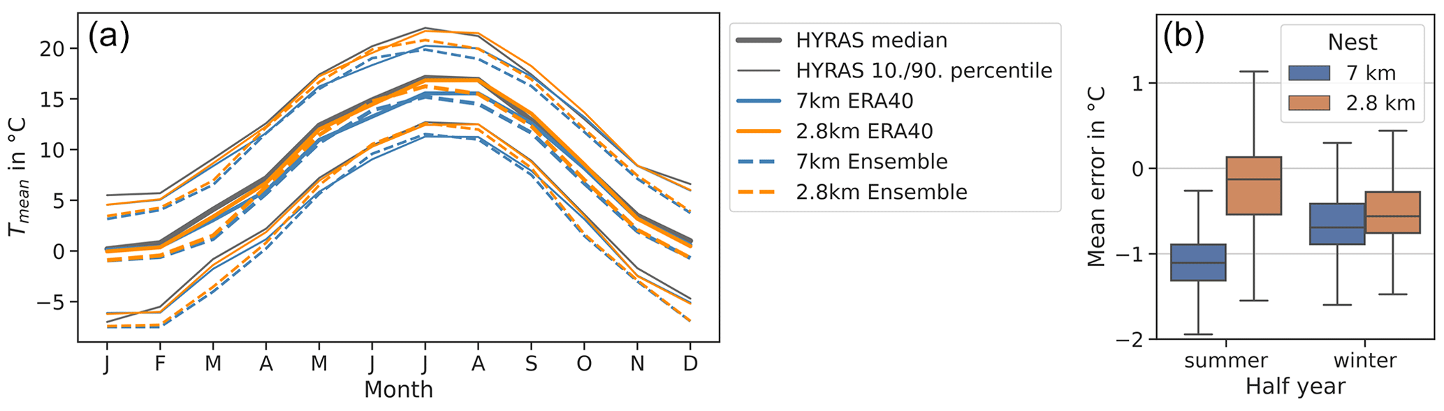
Figure 3 Raw output of 2 m temperature in the second (7 km) and third grid (2.8 km) in comparison with the observation dataset HYRAS for the reference period. The analysis was performed on the grid points in the evaluation area. Panel (a) shows the monthly mean temperature in the observation (solid black lines) compared to the reanalysis results (solid colored lines) and the median of the ensemble members (dashed lines). The thick lines represent the median in the reference period and in the evaluation area, and the thin lines show the 10th and 90th percentiles, respectively. Panel (b) visualizes the mean error in ERA40 time series compared to the observations for summer (May–October) and winter half years (November–April). The boxplot shows the spread over the grid points.

Averaged over all grid points, the mean error in the reanalysis-driven simulations is reduced from −1.1 to −0.13 ^∘C in the summer half year (Fig. 3b). Moreover, the spread is increased. In the winter half year the median is reduced from −0.69 ^∘C for 7 km to −0.56 ^∘C for 2.8 km. This is a smaller but still significant reduction confirmed by a Wilcoxon signed-rank test. The test was applied to the two fields of mean error in the coarser-resolution (7 km) and convection-permitting (2.8 km) simulations. The null hypothesis of zero difference between the errors was rejected by the test based on a significance level of 0.05. Those patterns in the temperature output from coarse to high resolution are similar in the ensemble as in the reanalysis-driven run. For further information on the performance of the single ensemble members, please refer to the Supplement (Fig. S1).

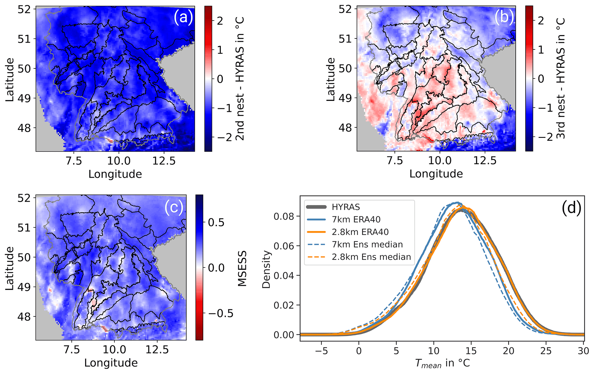
Figure 4 Evaluation of ERA40-driven simulation on a convection-parametrizing (7 km) and a convection-permitting (2.8 km) scale for the summer half year (May–October) in the period 1971–2000 compared to the reference observation data from HYRAS. The difference in the raw output of mean summer temperature is shown (a) for the 7 km simulation and (b) for the 2.8 km simulation. In (c) the MSESS of 2.8 km compared to 7 km is mapped, and (d) displays the density distribution of 2.8 and 7 km in the evaluation area for the reanalysis-driven run (solid lines) and the median of the ensemble in the reference period (dashed lines).

To reveal spatial patterns, the mean summer half-year temperatures of the second 7 km nest (Fig. 4a) and the third 2.8 km nest (Fig. 4b) of the reanalysis-driven run are compared to the observations (Fig. 2a). Whereas there is a negative bias at nearly all grid points for the coarser nest (Fig. 4a), local differences are visible for the convection-permitting simulation (Fig. 4b). Here, a negative bias is still present in the north of the domain, especially in the hilly regions. In the south of Germany, predominantly positive anomalies are visible. Even though the regions with positive bias are not correlated with altitude, they do not seem to be independent of orography. The largest positive bias is found in the South German Scarplands (long ≈ 9.0^∘, lat ≈ 48.5^∘) – located directly between two major mountain ridges: the Black Forest and the Swabian Alps.

For nearly all grid points, there is an improvement with the convection-permitting simulation, which is indicated by a positive MSESS in Fig. 4c comparing the second and third nest with respect to the reference dataset HYRAS. There are a few grid points with negative MSESS. Those are associated with a positive bias and an overshoot of the convection-permitting simulation.

The density distribution of daily summer temperature shows nearly perfect agreement of observation and the convection-permitting reanalysis run (Fig. 4d). In comparison, the distribution for the reanalysis-driven 7 km simulations is shifted towards colder temperatures and has a lower spread. Especially the highest summer temperatures are better resolved by convection-permitting simulations. An improvement is also visible for the 2.8 km median of the ensemble simulations compared to the 7 km output. However, especially the high summer temperatures are still underestimated by the CPM. Low temperatures, from approximately −3 to 10 ^∘C, are overestimated.

Overall, we identify a significant reduction in the mean bias for the convection-permitting resolution, which is especially pronounced during summer. Over Germany, the convection-permitting simulation reproduces a realistic frequency distribution of daily 2 m temperature. The remaining mean errors show a trend from negative bias in the north toward positive bias in the south. Other local patterns are partly associated with the predominant landscape regions. Based on the added value found in the 2.8 km resolution, its output is used for the following analysis.

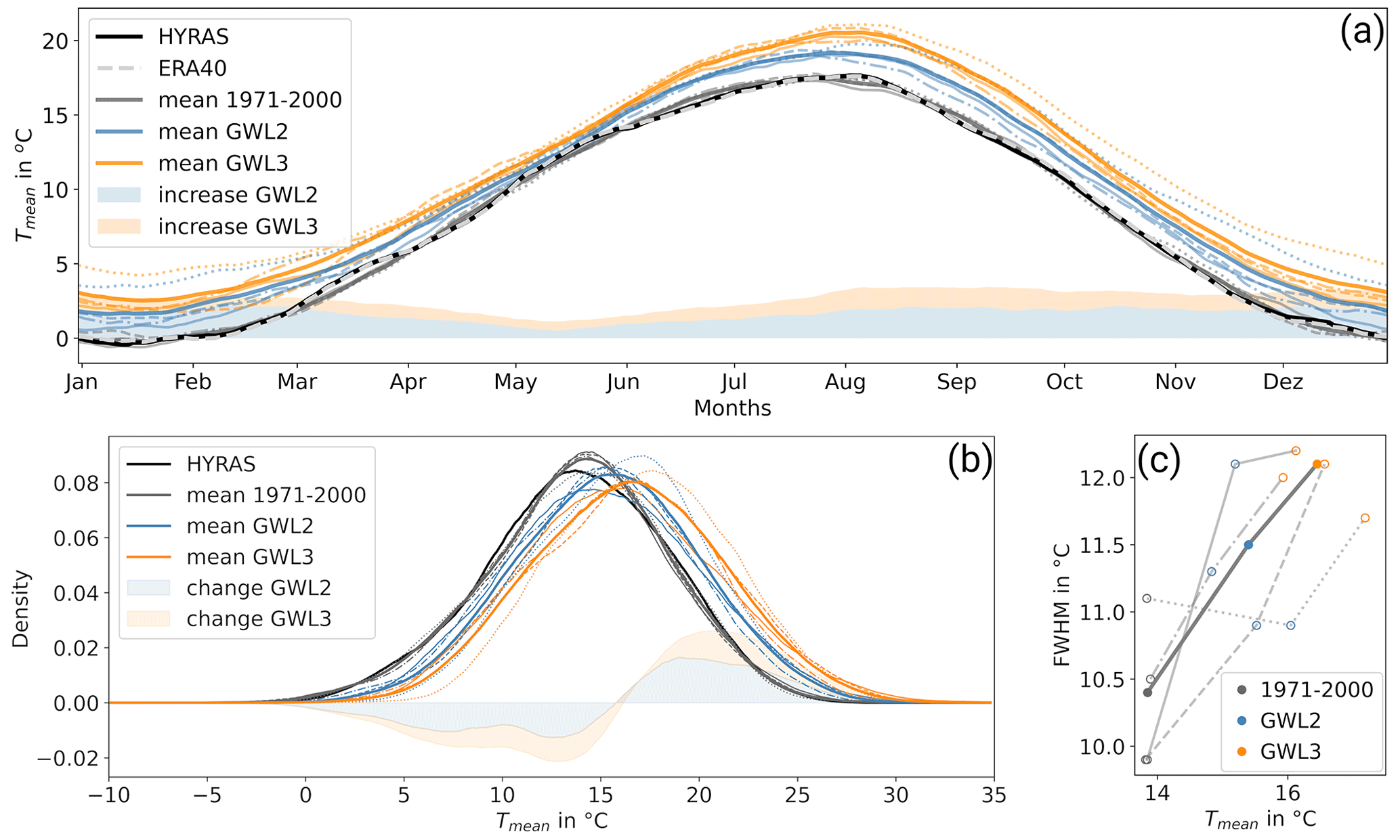
Figure 5 The different aspects of the evolution of daily mean temperature T_mean from the reference period (grey) over GWL2 (blue) to GWL3 (orange) are shown. Panel (a) displays its annual cycle averaged over the study area and over a 31 d running window. Panel (b) shows the density distribution of daily mean temperature in the summer half year (May–October) and (c) its full width at half maximum (FWHM). Different line styles correspond to different driving GCMs – solid: MPI-ESM-LR; dashed: EC-EARTH; dash-dotted: CNRM-CM5; dotted: HadGEM2-ES; the thick lines correspond to the ensemble mean.

4 Regional temperature trends

4.1 Annual cycle

Future temperature is not expected to develop evenly over the year. In the study area, the smallest increase is observed in spring and the largest in late summer and during winter (Fig. 5a). The behavior is similar for GWL2 and GWL3. The stronger late summer increase leads to a shift in the summer peak of maximum temperature by 12 d in GWL3 compared to 1971–2000.

A closer view of the ensemble spread shows that throughout the year, there seems to be good agreement within the three simulations driven by EC-EARTH, MPI-ESM-LR, and CNRM-CM5. There is an ensemble variance of 0.6 ^∘C² for the mean temperature averaged over the study area in GWL3. In contrast, warming – especially in the winter and autumn – is significantly more pronounced in the simulation driven with HadGEM2-ES (Fig. 5a, dotted line). Averaged over the year, the temperature increase is 1.5 ^∘C higher than for the other simulations by GWL3. HadGEM2-ES is the member with the highest climate sensitivity of the driving GCM within this ensemble (see Nijsse et al., 2020; Table 1). In the following, the presented results of HadGEM2-ES will stand out repeatedly as it appears that the nature of its projected climate change signal differs from that in the other three ensemble members EC-EARTH, MPI-ESM-LR, and CNRM-CM5 with lower climate sensitivity.

4.2 Temperature distribution

Figure 5b shows the density of the daily mean summer temperatures over the evaluation area. The peak of the distribution in the evaluation period is at 14.2 ^∘C. The shape of the distribution is reproduced well compared to the observations; however, the ensemble overestimates the probability at the peak of the distribution. In a warmer world, the mode shifts to higher temperatures that are 15.4 ^∘C in GWL2 and 16.6 ^∘C in GWL3. Moreover, higher maximum temperatures up to 27.4 ^∘C (99th percentile) in GWL3 are reached. There is a decline in temperatures left of the peak. However, especially for low temperatures, the magnitude of decrease is relatively small, leading to an increased width of the distribution. A parametrization of the spread of the distribution is made in terms of the full width at half maximum (FWHM), which is defined as the width of the distribution at the level of the half-peak value. As shown in Fig. 5c the FWHM in the ensemble average increases from 10.4 to 12.1 ^∘C. Three out of four ensemble members agree on a steady increase in the width. Only the simulation run by HadGEM2-ES does not confirm an increase in FWHM in the period from 1971–2000 to GWL2. Regarding the temperature distribution, an increasing FWHM indicates a more variable daily temperature, leading to higher amplitudes and to a stronger increase in the frequency of warm extremes on the right side of the curve compared to the shift in the curve median.

4.3 Spatial patterns

The average summer temperature (May–October) varies significantly over the evaluation area as already shown for the observational data in Fig. 2a and provided in the Supplement (Fig. S2) for the ensemble mean. It ranges from 12.3 to 15.5 ^∘C (5th and 95th percentile). As expected, the highest temperatures are found at low altitudes. The Rhine Valley stands out with the highest average temperatures up to 16.6 ^∘C. The lowest average temperatures are accordingly observed in complex regions with pronounced orography: examples are the Harz (average 12.5 ^∘C) in the Central Uplands and the Black Forest (average 13.0 ^∘C) in the south. Moreover, spatial heterogeneity is increased in those complex regions.

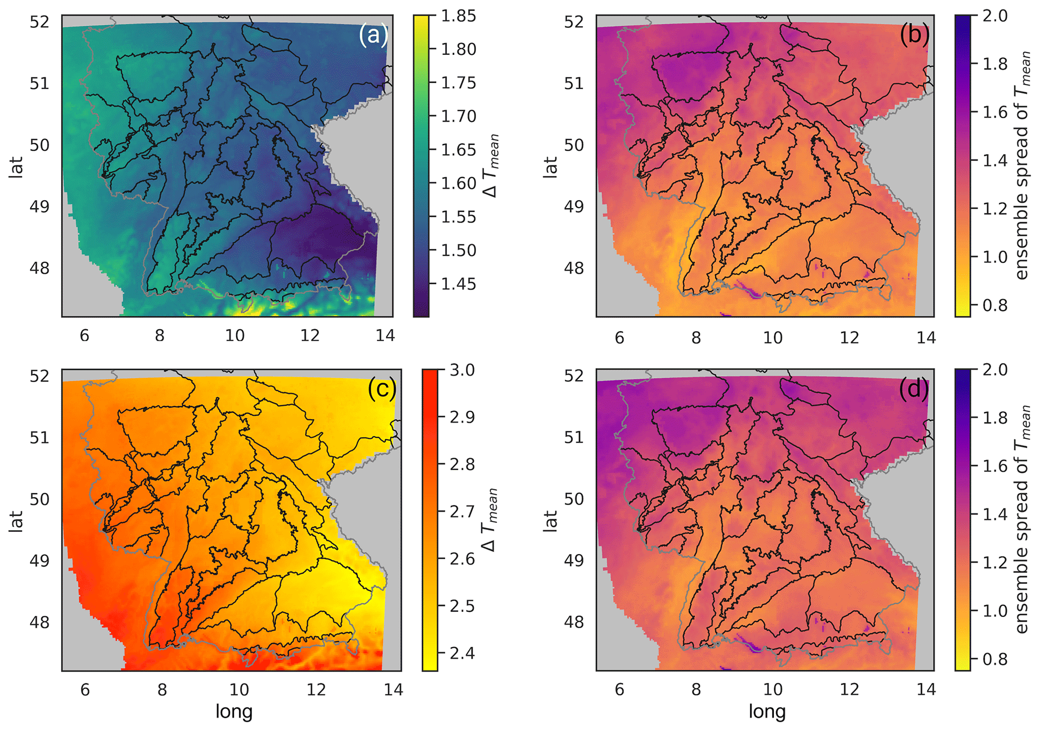
Figure 6 Mean development of T_mean in the summer half year (May–October) as an ensemble mean compared to the reference period for GWL2 (a) and GWL3 (c) and the corresponding ensemble spread calculated as a range between minimum and maximum prediction for each grid point in GWL2 (b) and GWL3 (d).

The summer temperature increases with global warming over the whole evaluation area. From the reference period (global warming at 0.46 ^∘C) to GWL2, the increase is on average 1.55 ^∘C (Fig. 6a). From the reference period to GWL3, the average increase is 2.60 ^∘C (Fig. 6c). When integrated over the year, the ensemble shows a slightly stronger warming than only over the summer months, indicating that summer temperatures are less sensitive than the annual mean (Fig. 5a). However, the differences are still in the range of 0.11 ^∘C (0.09 ^∘C) above the global warming in GWL2 (GWL3). Therefore, the regional warming in the evaluation area in the considered GCM–RCM combinations is close to the global average and only slightly enhanced. This is less than suggested by the theory of greater warming over land than over the ocean and as generally projected (IPCC, 2023). The impact of the bias correction is considered to be negligible, as the uncorrected data integrated over the year show a nearly identical warming of 0.11 ^∘C (0.07 ^∘C) above the global average in GWL2 (GWL3) in the evaluation area.

Geographical dependence leads to regional variations in warming. Over the evaluation area, warming ranges from 1.45 to 1.64 ^∘C (5th and 95th percentiles) in GWL2 and from 2.44 to 2.76 ^∘C in GWL3. As shown in Fig. 6a and c, the strongest increase is observed in the uplands in the north of the domain (GWL2) and in the Black Forest and Swabian Alps in the south (GWL2 and GWL3). Less warming, below the global average, is expected in the Alpine Foreland (GWL2 and GWL3).

The ensemble spread increases from GWL2 with 1.06 to 1.47 ^∘C to GWL3 with 1.12 to 1.48 ^∘C (5th and 95th percentile). Data show a trend superimposed from north to south with decreasing spread (Fig. 6b and d). Moreover, the ensemble spread seems to depend partially on the orography and landscape. It is especially high in the northwest of the domain and in areas with higher elevation. The lowest spread is visible in the flat Rhine Valley. The higher deviations at the locations of the large lakes in southern Germany – Lake Constance (long 9.4; lat 47.6), Lake Ammersee (long 11.1; lat 48.0), Lake Starnberg (long 11.3; lat 47.9), and Lake Chiemsee (long 12.5; lat 47.9) – are caused by interpolation of the water surface temperatures from the coarse grid, since no lake module was applied.

Summing up, the mean temperature over Germany rises in a warmer climate predominantly in late summer as well as in the winter half year, with the smallest increase in spring. This leads to a general shift in the summer maximum temperatures to later summer. The increase is spatially largely homogeneous, with slightly stronger warming expected in mountainous regions. Moreover, the temperature distribution in a warmer climate is expected to be wider (larger variability), indicating that extreme temperatures will experience a greater change compared to the average warming.

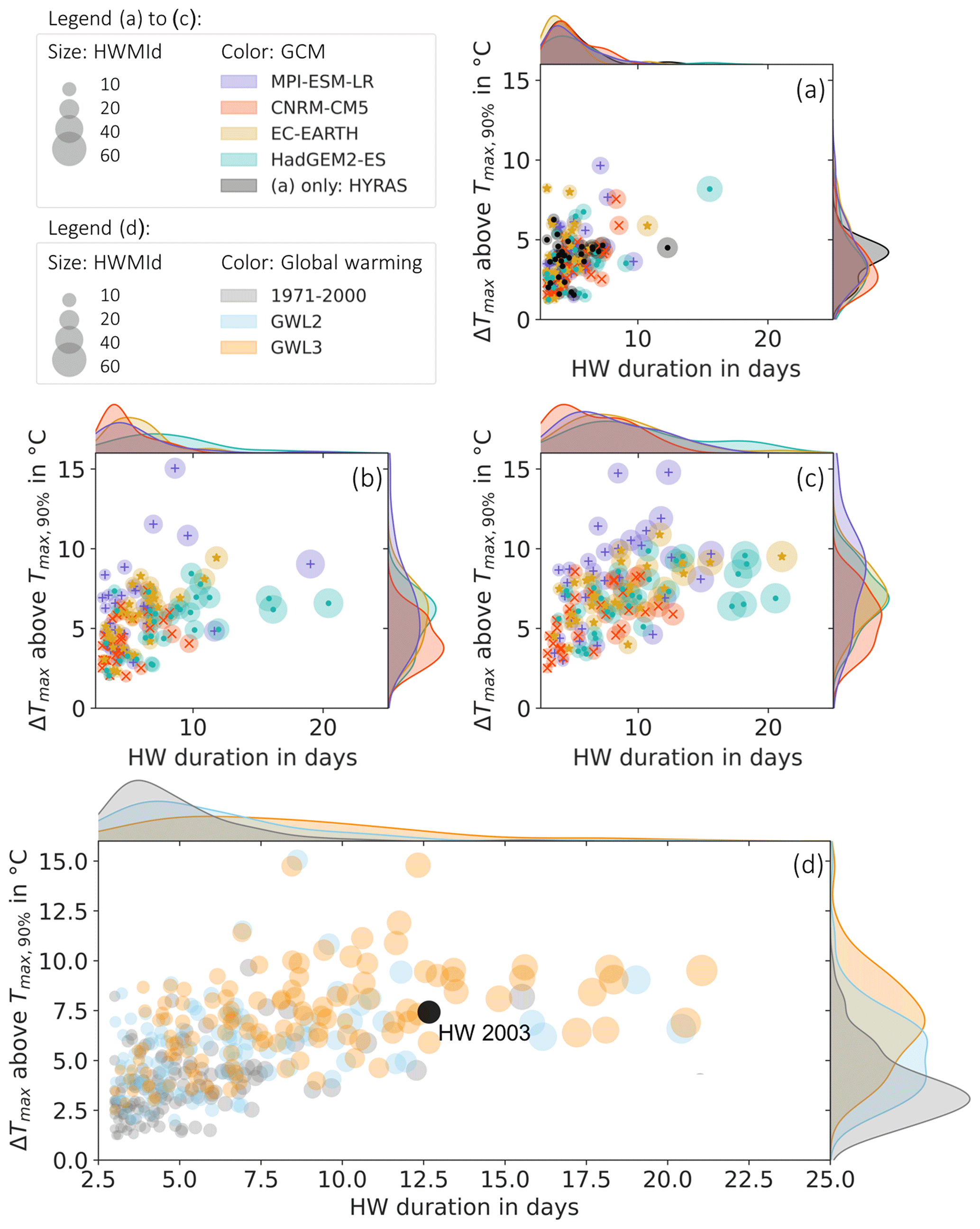
Figure 7 The bubble plots show the strongest HW in each summer half year (May–October) in every projection run with respect to duration on the abscissa and excess temperature on the ordinate. Bubble size indicates mean HWMId over all grid point results affected by the HW. Marginal plots show the distribution of duration of the heat waves in days (abscissa) and the distribution of the excess temperature (ordinate). Panels (a)–(c) show the single ensemble members and comparison with the observation: (a) for 1971–2000, (b) for GWL2, and (c) for GWL3. Panel (d) shows the total set of all of the heat waves from the single ensemble members for 1971–2000, GWL2, and GWL3. The black data point corresponds to the HW in 2003 derived from HYRAS data.

5 Heat wave characterization

This section characterizes HWs in the future based on their different features – length, temperature, magnitude, and frequency. Be aware that throughout this section we are focusing on a relative definition of these events – an anomaly versus the 90th percentile from the reference period (Sect. 2.3.1). The relationship between HW magnitude, duration, and excess temperature is examined for the most severe HWs in each year in terms of the cumulative HW magnitude in the evaluation area (Fig. 7). The corresponding figure providing absolute HW temperatures is provided in the Supplement (Fig. S3).

Firstly, the observed HW characteristics in the reference period (1971–2000) are analyzed, as shown in black in Fig. 7a. The average duration of the strongest HWs per year ranges from 3 to 12 d. The temperature excess ΔT_max above the 90th percentile ranges from 1.5 to 6.3 ^∘C. The longest observed HW reaches up to 12 d; however, the correlation with excess temperature is weak (r=0.22). The observed HWMId has a range of 5 to 22, with an average of 8.8. HWMId increases with HW length (r=0.99).

To evaluate the representation of the three HW characteristics in the ensemble projection, the results of observation and simulations in the reference period are compared (Fig. 7a). The HW duration is reproduced well by all ensemble members, and no significant deviation from the observed distribution of duration (marginal distribution on the abscissa) is visible, which is confirmed by a two-sample Kolmogorov–Smirnov test at the level of significance of 0.05. Also for the HWMId, the test confirms no significant deviation between simulation and observation. For the excess temperature, no significant deviation from the observed distribution is found for three out of four ensemble members. However, significant differences for the results of the CNRM-CM5-driven simulation and an underestimation of the simulated excess temperature are visible in the marginal distribution on the ordinate (Fig. 7a). Moreover, there is a peak around ΔT_max=4 ^∘C in the observation that is not reproduced by any ensemble member. The ensemble of climate simulations shows no significant deviation from the observed distributions in the reference period for the characteristic duration and HWMId, confirmed by a two-sample Kolmogorov–Smirnov test at a level of significance of 0.05. For the excess temperature, the test results support no significant deviation from the observed distribution for three out of four ensemble members but significant differences for the results of the CNRM-CM5-driven simulation. The underestimation of the modeled excess temperature is shown in Fig. 7a. Moreover, a peak around ΔT_max=4 ^∘C is visible in the observation that is not reproduced by any ensemble member.

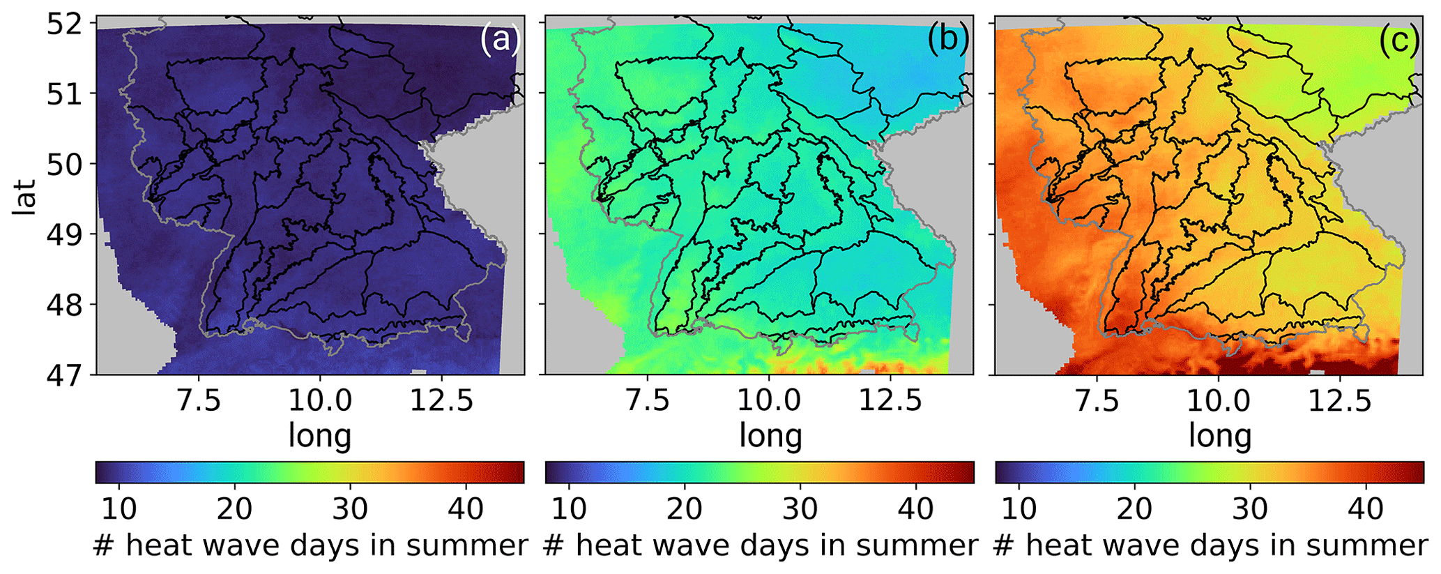
Figure 8 The ensemble mean of the average number of HW days per summer half year (May–October) in 1971–2000 (a), GWL2 (b), and GWL3 (c).

The climate change signal of excess temperature (1), duration (2), and magnitude (3) develops differently in the four ensemble members (Fig. 7b and c), but when superimposing the three GWLs, a clear picture of HW intensification emerges (Fig. 7d). (1) All ensemble members agree on an increase in average excess temperature and an increased width of its distribution compared to the reference period. The highest excess temperatures are found for MPI-ESM-LR-driven simulation up to ΔT_max=15 ^∘C in GWL2 and GWL3. The lowest excess temperatures are projected by the simulation driven by CNRM-CM5 that already showed an underestimation in the reference period. In the ensemble median, there is a shift towards higher HW excess temperatures up to 5.3 (GWL2) and 6.9 ^∘C (GWL3) (Fig. 7d). This implies that with HW excess temperatures from 2.6 to 4.5 ^∘C (25 % and 75 % confidence interval) in the reference period, hardly any HWs are occurring today that will be a common scenario in the future. (2) Also for HW duration, a future increase in mean and spread of the distribution is detected by all ensemble members. Again, the smallest changes are projected by the simulation driven by CNRM-CM5. The simulation driven by HadGEM2-ES projects in general the longest HWs. These discrepancies in HW duration indicate different dynamics in the driving models. In fact, HadGEM2-ES is described as one of the best-performing CMIP5 GCMs for past climates and weather types (Perez et al., 2014), as well as blocking, which is underestimated in CMIP5 models in general (Brands, 2022). The extremely long HWs presented should therefore not be discounted as outliers but treated with caution. In the ensemble average, there is a clear shift towards longer HWs. The average duration increases from 4.3 (reference) over 5.1 (GWL2) to 7.5 d (GWL3). Moreover, the spread increases drastically, which leads to maximum HW duration up to 21 d. (3) The development of HWMId is strongly correlated with HW duration in the simulations. In the ensemble, a 26 % (100 %) increase in the median of HWMId is expected from the reference to GWL2 (GWL3) (HWMId in the reference: 8.2; GWL2: 10.3; and GWL3: 16.5). The significance of the increase in duration, excess temperature, and HWMId is confirmed by a two-sample Kolmogorov–Smirnov test at the level of significance of 0.05.

In order to put the results into perspective, they are compared with an actual reference event for Germany – the HW in 2003. The HW had a strong economic and environmental impact, caused a thousand deaths, and is referred to as a record HW (e.g., De Bono et al., 2004). Performing an analog analysis on 2003 HYRAS data, this HW had an average length of 12.7 d, maximum excess temperature of 7.4 ^∘C, and HWMId of 26.7. It is visualized in black in Fig. 7d. As expected the event is extremely unlikely in the reference period. Only one simulated summer in the reference period by HadGEM2-ES exceeds the measured event in 2003. In a warmer world, events with such a strength occur with higher probability. In GWL3 such an event is in the 25 % confidence interval of 5.3 to 8.4 ^∘C. For duration, the HW 2003 exceeds the 25 % confidence interval of 5.1 to 10.4 d in GWL3, and its duration is ranked 16th in the projections of 4×30 years, corresponding to an 8-year return period in GWL3. For HWMId, its rank of 21 in GWL3 leads to a 6-year period. It should be noted that in this case no distinction is made between ensemble members. The variations between ensemble members discussed earlier indicate the range of uncertainty in this projection. Moreover, the analysis considers only the local observations of 2003 limited to the simulation area. Summing up, an event like HW 2003 will become more likely but is projected to stay an extreme event with a return period of 5 to 10 years.

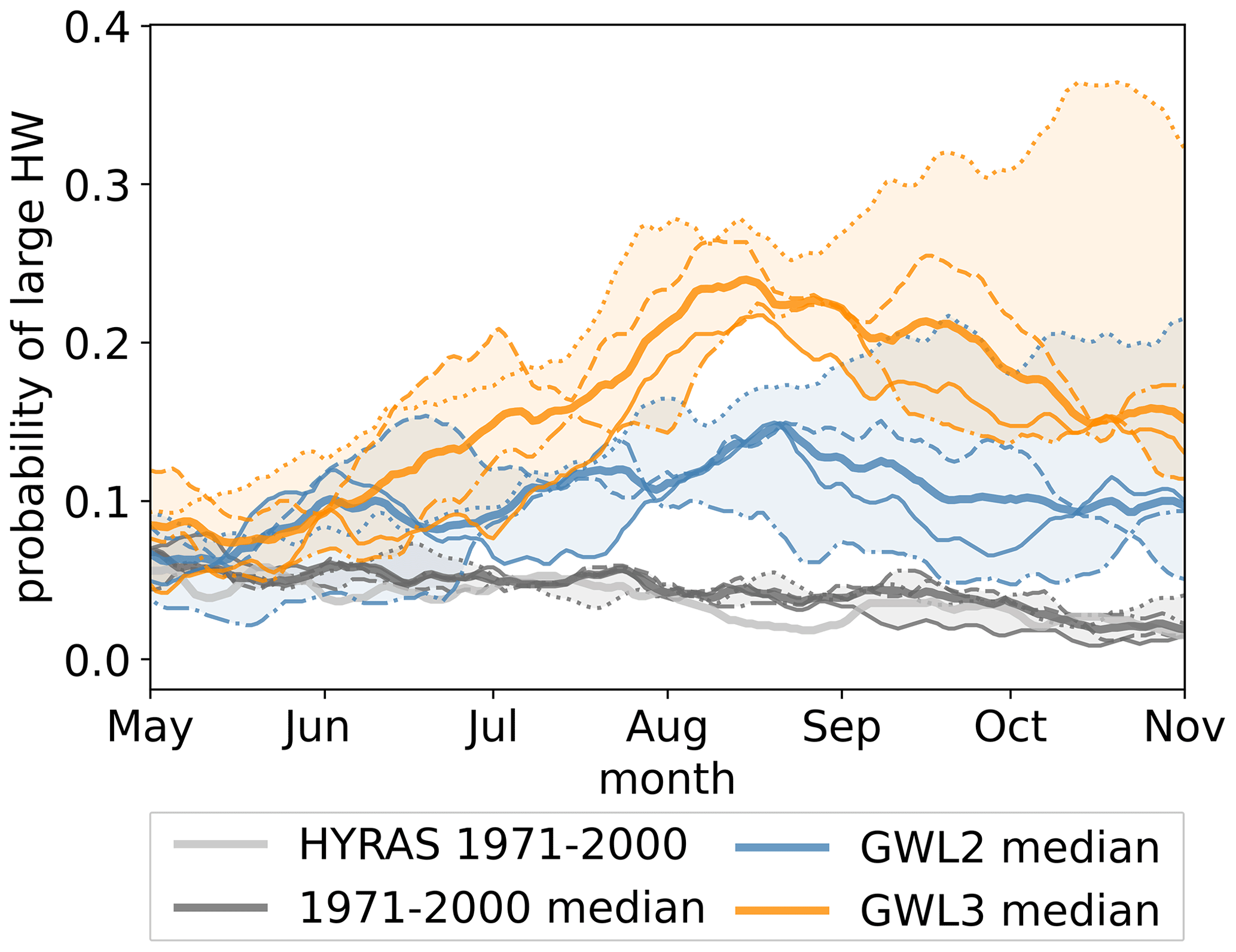
Figure 9 Probability of large HWs (coverage ≥ 50 % of the evaluation area) over the summer (May–October) calculated over a 31 d running window. The thick line corresponds to the ensemble median, whereas the different line styles of the thin lines correspond to different driving GCMs – solid: MPI-ESM-LR; dashed: EC-EARTH; dash-dotted: CNRM-CM5; dotted: HadGEM2-ES.

To assess regional patterns, the cumulative number of HW days as a measure of HW frequency is analyzed (Fig. 8). Again the summer half year is considered only. In the reference period, averaged over 30 years, few HW days are observed per summer half year. In the evaluation area, the number of HW days ranges from 8.7 to 9.9 (5th to 95th percentile) and is distributed relatively uniformly across space. An overall increase from 18.8 to 23.0 (5th to 95th percentile) HW days is simulated in GWL2. With even more warming in GWL3, spatial features become visible. The increase predominantly affects the southwest. Moreover, slightly enhanced HW occurrence is projected in regions with higher elevation like the Black Forest. Over the domain, 28.7 to 36.9 (5th to 95th percentile) HW days are expected in GWL3.

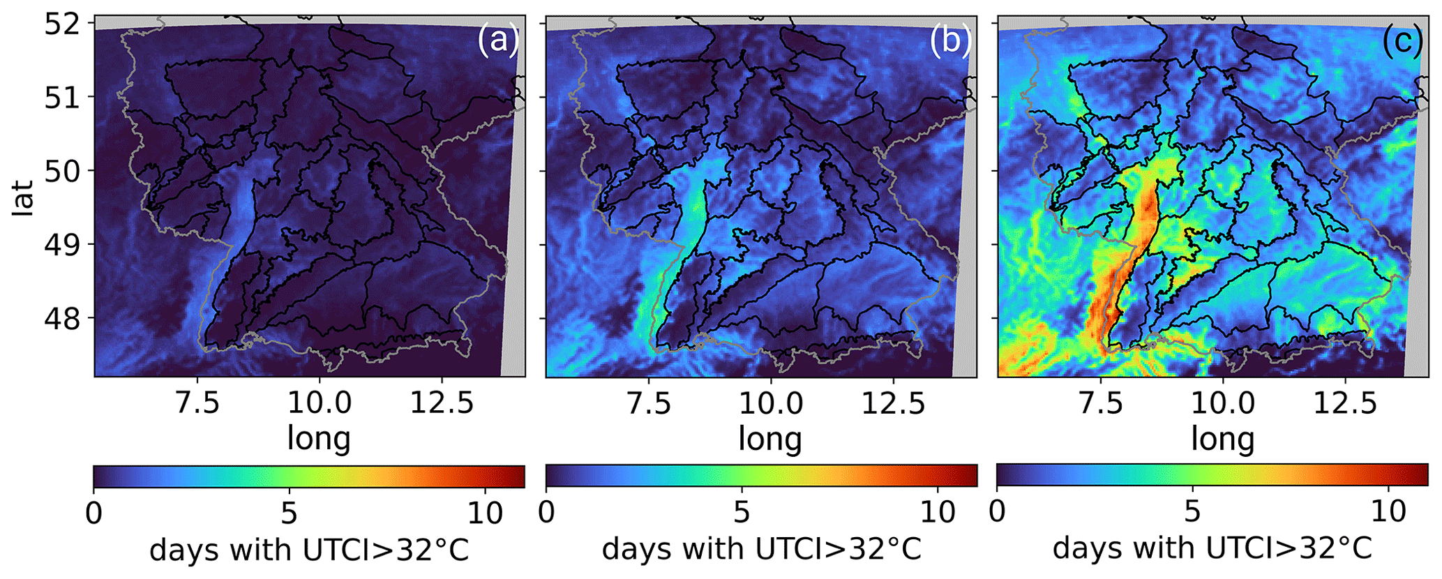
Figure 10 Ensemble median of the number of days per year with strong human heat stress defined by UTCI > 32 ^∘C for 1971–2000 (a), GWL2 (b), and GWL3 (c).

The analysis of the seasonal changes reveals that HW severity is distributed inhomogeneously over the summer (Fig. 9). In the reference period the occurrence of large HWs, defined as HWs with a coverage of at least 50 % of the study area, is relatively flatly distributed. There is a declining trend of the probability throughout the summer. From GWL2 to GWL3, it is apparent that there is an increased HW occurrence in late summer, around August and September. All members of the ensemble agree on this trend. However, the magnitude and timing of the adjustment vary. The highest HW probabilities are projected by EC-EARTH and HadGEM2-ES. Some ensemble members even depict a decrease in the occurrence of large HWs in early summer in GWL2 (May to June).

The analysis of both regional and seasonal patterns supports HW frequency as being closely linked to the future temperature increase, for which a similar spatial pattern and annual cycle of the change signal were found. However, it should be noted that, while the average temperature increases by only 2.6 ^∘C from the reference period to GWL3 (Sect. 4), this translates into an enormous increase in HW frequency of more than a factor of 3. This amplified increase in HW frequency is attributed mainly to a higher change of higher percentiles compared to the increase in mean temperature (Sect. 4). Furthermore, more persistent weather patterns potentially enhance the severity of HWs in a future climate (Kyselỳ, 2008).

In summary, future HWs are characterized by significantly higher temperatures and longer HW duration. Thus, the magnitude of HWs increases dramatically in a warmer future, namely by 26 % (100 %) in GWL2 (GWL3). Furthermore, enhanced variability is projected for the HW characteristics. While the increase in HW days is spatially largely homogeneous, there is clear seasonality, with a strong increase in HW occurrence in late summer.

6 Impacts of temperature and heat increase

The meteorological perspective leaves open the question of the impacts of heat extremes, which will be addressed in the following section. The focus is first on human heat stress, and then the analysis is extended to further heat-related climate parameters.

6.1 Human heat stress

The number of days with UTCI > 32 ^∘C is defined as days with strong human heat stress. As outlined in “Data and methods”, UTCI is derived from hourly data. Due to missing gridded hourly observations, it was not subjected to bias correction. As a consequence, there is a larger ensemble spread in the UTCI. There is good agreement between three of the four ensemble members, showing a similar range of UTCI over the reference period 1971–2000. The simulation driven by HadGEM2-ES results in a significantly higher number of days with UTCI > 32 ^∘C. We attribute this difference mainly to higher summer temperatures in this simulation, which unlike the previous analysis of daily data was not subject to bias correction. To minimize the influence of possible outliers, we consider the ensemble median in the following analysis. The spatial distribution is displayed in Fig. 10. In the reference period hardly any days per year with strong heat stress are found. The range over the evaluation period is 0.0 to 0.6 d yr⁻¹ (5 % to 95 % confidence interval). A maximum number of up to 2.0 d yr⁻¹ averaged over the reference period in flat regions is visible in the ensemble.

The average number of days with strong heat stress rises in the future GWL2 all over the domain – on average by 0.6 d yr⁻¹ – but with notable spatial differences. Again the highest numbers of heat stress days are in the flat Rhine Valley with up to 5.1 d yr⁻¹ (Fig. 11a). Moreover, this region shows the strongest increase from the reference to GWL2, which is on average 1.8 d yr⁻¹. For GWL3, this pattern intensifies with a nonlinear, rather exponential increase with global warming (Fig. 11a). Up to 10.7 d yr⁻¹ with strong heat stress is projected in the hottest region. Also in regions with higher elevation, there is a significant increase in future heat exposure; on average 2.3 d are for example expected in the Black Forest by GWL3. For comparison, this exceeds the heat stress that prevailed in the mild, flat Rhine Valley during the reference period.

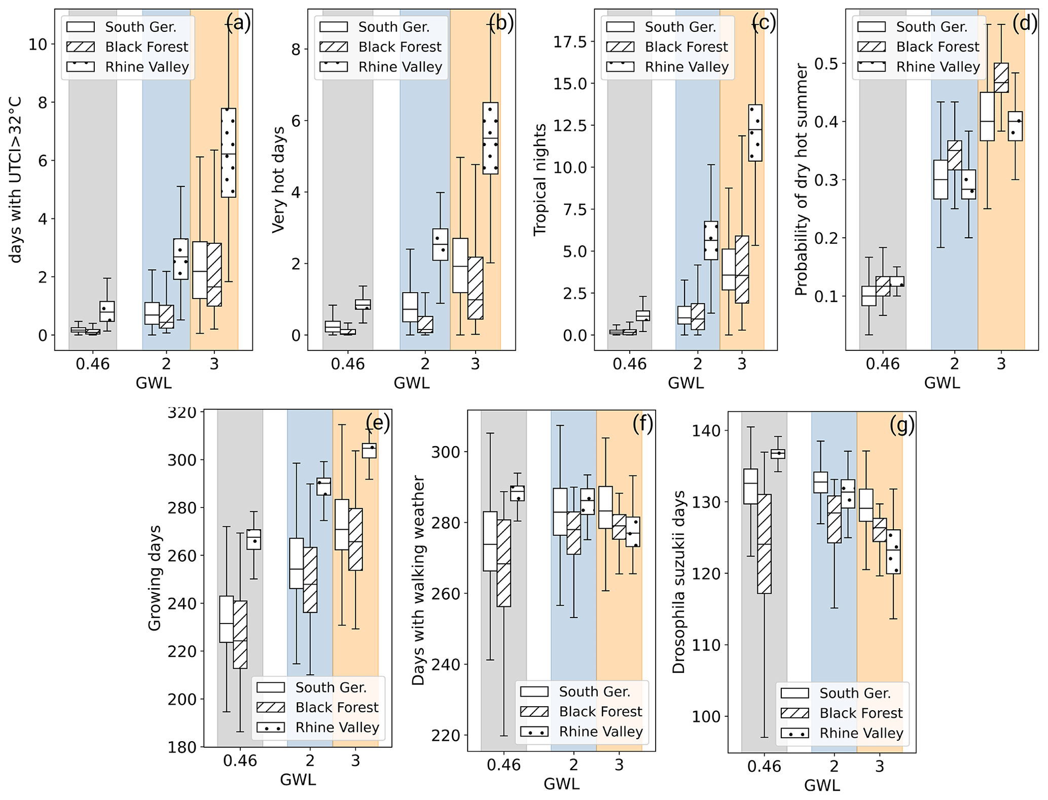
Figure 11 Ensemble median of UTCI and climate parameters over global warming. The global warming level of the reference period is assumed to be 0.46 ^∘C based on Teichmann et al. (2018). The empty boxplot visualizes the distribution over the evaluation area, and striped boxes represent results in the Black Forest and dotted in the Rhine valley.

6.2 User-tailored climate parameters

The analysis of the six tailored climate parameters shows how changing temperature affects further fields of action (Fig. 11b–g). To visualize regional effects, results of two German landscape regions are added to the graph in addition to the entire evaluation area: the flat and warmest region of the model domain, the Rhine Valley (dotted boxes), and its counterpart the Black Forest region (striped boxes), which is geographically directly adjacent to the Rhine Valley and, as a low mountain range, has a high altitude and complex orography (see Fig. 1).

The most drastic changes in the mean values are projected for very hot days, tropical nights, and dry hot summers (Fig. 11b–d). In addition, for very hot days and tropical nights a nonlinear, rather exponential increase with global warming is projected. This coincides with a significant increase in variance. The behavior of very hot days and tropical nights is comparable to UTCI (Fig. 11a), implying that this amplified, nonlinear increase might be preferentially associated with strong heat stress. The pattern is observed for all shown landscape regions. Differences appear in the absolute values: heat stress is especially pronounced in the Rhine Valley at low altitude where it exceeds the values in the adjacent Black Forest by a factor of 3.7 (very hot days) or 2.8 (tropical nights) in GWL3.

An approximate mean linear increase with global warming is visible for dry hot summers and growing days (Fig. 11d and e). Growing days are expected to increase on average by 39 (evaluation area), 40 (Black Forest), and 37 (Rhine Valley) days from the reference to GWL3, indicating that dependency of the change signal on the region is negligible. Existing regional patterns and variability within a landscape region appear to be preserved in a warmer climate, and mean values are subjected to a shift only.

The probability of dry hot summers increases approximately linearly as well, accompanied by increasing spatial variance. Here, the largest increase is observed in the Black Forest and the smallest in the Rhine Valley. Overall, the probability of a dry hot summer increases drastically: from the reference to GWL3, the projected mean increase corresponds to a factor of 4 (evaluation area and Black Forest) or 3.2 (Rhine Valley).

The two remaining parameters are examples designed for specialized applications in individual, often region-specific challenges – here walking weather for tourism strategy (Fig. 11f) or pests, e.g., Drosophila suzukii, for agricultural planning (Fig. 11g). Using days with walking weather as an example, their number increases in the Black Forest and the variability decreases. The trend in the Rhine Valley is opposite: a decreasing number of days with walking weather with increasing variance. Hence in GWL3, relatively similar numbers of days are to be expected in the two contrasting regions. Also for days with conditions for Drosophila suzukii, no common trend can be identified, and the examples show a climate change signal that depends crucially on local conditions. Such behavior is mainly attributed to the more complex definition of the parameters with an upper and a lower limit. The evaluations indicate that the more complex the parameter – or the underlying challenge in climate adaptation – the more important the regional consideration becomes.

We conclude that the changes regarding UTCI and user-tailored climate parameters do not necessarily scale linearly with global warming. An overproportional increase in the climate parameter with global warming is preferably the case for parameters that describe strong heat stress. Moreover, the change signal of climate parameters depends crucially on the landscape region. In particular for parameters describing strong heat stress, the absolute change signal is highest in flat regions that are already exposed to the greatest heat today. For specialized applications, parametrized over more complex climate parameters, region-specific trends are expected.

7 Discussion and conclusion

In the presented analysis of heat extremes and related impacts in a convection-permitting climate ensemble for Germany, we can draw three main conclusions:

1. We found an added value for simulated temperature in the convection-permitting ensemble, especially for hot temperatures, that goes beyond better representation of the topography only. The improvement is particularly prominent in the summer half year.

2. Mean temperature in the warm season in Germany increases largely homogeneously in space. An increase in temperature variability is found in future projections, which favors the development of longer and hotter HWs, especially in late summer. Heat wave magnitude is expected to increase by 26 % (100 %) in GWL2 (GWL3).

3. The changes in human heat stress (UTCI) and tailored climate parameters show a clear dependence on the major landscapes. Heat stress is particularly prominent for lowland areas like the Rhine Valley. An overproportional increase in parameters associated with strong heat stress is found. For the change signal of more complex tailored climate parameters, linear behavior and/or strong dependency on the landscape can be identified.

Our results show an improved representation of the 2 m temperature in the raw CPM output compared to the coarser 7 km grid with parametrized convection. The improvement found is largest in the summer, when the cold bias in the coarser simulation was substantially reduced. This applies to both the median temperature and the more extreme percentiles (10th and 90th) of the temperature distribution over the model domain in the historical period. The improvement found in the temperature output on the convection-permitting scale confirms the findings by Hackenbruch et al. (2016), Hohenegger et al. (2008), and Laube (2019). However, recent studies have shown that this temperature bias, especially in daily minimum and maximum, can still be addressed in CCLM with an improved formulation of the 2 m temperature in the land surface scheme (Schulz and Vogel, 2020). Moreover, it needs to be clarified whether the improved temperature output in the convection-permitting simulation justifies the higher computational cost for high-resolution simulations. While systematic biases between raw model temperature output and observations remain in our CPM ensemble, we show a clear benefit from a relatively large simulation area across different landscapes. We find a dependency of the remaining error in the landscape type and an association with orography – especially in transition areas between different major landscape types. Therefore we support a region-specific magnitude of the added value as in Soares et al. (2022). In order to provide information for climate change impact studies or user-oriented studies, in this case focusing on heat stress, there is still a need for bias correction. Especially for threshold-based parameters, bias correction is a necessity to obtain meaningful values. Nevertheless, we expect that such studies will benefit from the better representation of high temperatures on the convection-permitting scale due to the smaller impact of bias correction and thus a smaller source of error.

The analysis allows for the first time a very high-resolution projection of temperature and temperature extremes over Germany in a 2 and 3^∘C warmer world. The regional, high-resolution analysis confirms general warming over the whole region and a slightly higher change signal in mountainous regions. As in Vautard et al. (2014), the smallest temperature increase was found in spring. Indeed, the peak of summer temperatures in a warmer climate shifts to later in the summer. Moreover, the analysis confirms a wider distribution of temperature with global warming, implying a greater change in extreme temperature compared to the average warming in the future (e.g., Mearns et al., 1984; Schär et al., 2004; Giorgi et al., 2004; Kjellström et al., 2007; Vidale et al., 2007; IPCC, 2023). Our study shows that HW probability is expected to increase significantly over Germany, and especially in late summer large HWs are anticipated. HW severity is projected to rise dramatically, indicated by a 26 % (100 %) percent increase from 1971–2000 to a 2^∘C (3^∘C) warmer world. Increasing variability in HW characteristics is projected for the future. This is consistent with past trends of HW temperature and duration derived from observational data (Della-Marta et al., 2007). Our study thus suggests that the trend is likely to continue in the future.

Apart from meteorological insights, a closer look at human heat stress and other tailored climate parameters shows the potential of using convection-permitting simulations in different fields of application and highlights the importance of individual consideration. Strong human heat stress – parametrized via UTCI > 32^∘C and associated with very hot days or tropical nights – is prevalent in the flat regions such as the Rhine Valley. Moreover, the largest absolute increase is expected for these regions, comparable to Brecht et al. (2020). The change signal of tailored climate parameters does not always scale linearly with global warming – as is the case for the relative quantity of dry hot summers or growing days, a quantity that applies to moderate conditions. Especially for extreme heat stress (UTCI > 32^∘C, very hot days, or tropical nights) we see a nonlinear but rather exponential increase with global warming. In particular for specialized applications – expressed, e.g., over more complex climate parameters – behavior depends crucially on the prevailing landscape and might even lead to opposing trends. Therefore, the analysis supports previous results of spatial patterns (Schipper et al., 2019; Brecht et al., 2020) and shows the benefit of CPMs, which allows the representation of distinct characteristics in clearly defined areas.

The limitation of the study is that the assessment of uncertainty is restricted with four GCMs and only one RCM. However, the magnitude of the uncertainty associated with the RCM choice is typically smaller than from the large-scale GCM forcing (Kjellström et al., 2011). In the future, larger ensembles on the convection-permitting scales are expected to be available, enabling assessment of GCM and RCM uncertainty. Currently, ongoing downscaling of the CMIP6 GCMs is a promising source of future driving data for high-resolution climate simulations. In particular, the improved representation of Northern Hemisphere blocking in the new generation of climate models (Schiemann et al., 2020) will necessitate additional analysis of HWs and is anticipated to provide complementary insights to the results shown. Moreover, long convection-permitting projections would profit from the implementation of variable land surface characteristics over time, as, e.g., recently provided by FPS-LUCAS (Hoffmann et al., 2021). Moving from constant to variable input fields could yield valuable information for heat stress in impact studies. Especially for climate adaptation studies, development is still anticipated for urban areas and the evaluation of corresponding urban parametrization schemes. Since no parametrization is used in this study, further improvements for urban areas are to be expected (e.g., Trusilova et al., 2016; Daniel et al., 2019).

Heat extremes and related impacts derived from a convection-permitting ensemble document that the climate change signal depends on major landscape regions. Therefore, such convection-permitting projections have the potential to facilitate tailored impact studies and can help to narrow down the gap between climate research and the requirements of stakeholders, e.g., for sustainable risk management and climate adaptation. This presented finding stresses the need for climate adaptation strategies on a local level and supports the regional approach in climate adaptation research, e.g., in the German Federal Ministry of Education and Research (BMBF) RegIKlim project: basic research is done in a pilot region, concentrating on region-specific key issues to develop, evaluate, communicate, and test the implementation of adaptation strategies with the aim of an upscaling in the concerned region in the future.