Towards improving the spatial testability of aftershock forecast models

Aftershock forecast models are usually provided on a uniform spatial grid, and the receiver operating characteristic (ROC) curve is often employed for evaluation, drawing a binary comparison of earthquake occurrences or non-occurrence for each grid cell. However, synthetic tests show flaws in using the ROC for aftershock forecast ranking. We suggest a twofold improvement in the testing strategy. First, we propose to replace ROC with the Matthews correlation coefficient (MCC) and the F₁ curve. We also suggest using a multi-resolution test grid adapted to the earthquake density. We conduct a synthetic experiment where we analyse aftershock distributions stemming from a Coulomb failure (ΔCFS) model, including stress activation and shadow regions. Using these aftershock distributions, we test the true ΔCFS model as well as a simple distance-based forecast (R), only predicting activation. The standard test cannot clearly distinguish between both forecasts, particularly in the case of some outliers. However, using both MCC-F₁ instead of ROC curves and a simple radial multi-resolution grid improves the test capabilities significantly. The novel findings of this study suggest that we should have at least 8 % and 5 % cells with observed earthquakes to differentiate between a near-perfect forecast model and an informationless forecast using ROC and MCC-F₁, respectively. While we cannot change the observed data, we can adjust the spatial grid using a data-driven approach to reduce the disparity between the number of earthquakes and the total number of cells. Using the recently introduced Quadtree approach to generate multi-resolution grids, we test real aftershock forecast models for Chi-Chi and Landers aftershocks following the suggested guideline. Despite the improved tests, we find that the simple R model still outperforms the ΔCFS model in both cases, indicating that the latter should not be applied without further model adjustments.

1 Introduction

Aftershocks define earthquakes following a large earthquake (mainshock) closely in space and time. They can be as destructive or deadly as the mainshock or even worse. Therefore, right after the occurrence of a significant earthquake, an accurate probabilistic forecast of the spatial and temporal aftershock distribution is of utmost importance for planning rescue activities, emergency decision making, and risk mitigation in the disaster area. In addition to its use for operational earthquake forecasting to mitigate losses after a major earthquake, forecasts of the spatial aftershock distribution are also used to improve understanding of the earthquake triggering process by hypothesis testing.

The distribution of aftershocks is not uniform but associated with the inhomogeneous stress changes induced by the mainshock (Reasenberg and Simpson, 1992; Deng and Sykes, 1996; Meade et al., 2017). In particular, the spatial distribution of aftershocks generally correlates with positive Coulomb stress changes (King et al., 1994; Asayesh et al., 2019, 2020b). Numerous models for aftershock forecasting have already been proposed spanning the range of physics-based models (Freed, 2005; Steacy et al., 2005; Asayesh et al., 2020a), statistical models (Ogata and Zhuang, 2006; Hainzl, 2022; Ebrahimian et al., 2022), hybrid physics-based and statistical models (Bach and Hainzl, 2012), and machine learning models (DeVries et al., 2018). Those aftershock forecasts are usually provided in a discretized 3D space around the mainshock, including horizontal distances from the mainshock rupture, e.g. up to two fault lengths (Hill et al., 1993) or within 100 km (Sharma et al., 2020). The cell dimensions in 2D (also referred to as spatial cells) considered for previous studies are either 2 km × 2 km (Hardebeck, 2022), 5×5 km, 10×10 km (Sharma et al., 2020; Asayesh et al., 2022), or $\mathrm{0.1}{}^{\circ }\times \mathrm{0.1}{}^{\circ }$ (Schorlemmer et al., 2007).

Evaluating aftershock forecast models is a key scientific ingredient in the process of improving the models. It is desirable to use those forecast models for societal decision making that have proven their applicability through testing. A global collaboration of researchers developed the Collaboratory for the Study of Earthquake Predictability (CSEP) (Schorlemmer et al., 2007, 2018). Within this collaboration, many forecast experiments in various regions of the world have been implemented and evaluated (e.g. Schorlemmer and Gerstenberger, 2007; Schorlemmer et al., 2010; Zechar et al., 2010; Werner et al., 2011; Zechar et al., 2013; Strader et al., 2018; Savran et al., 2020; Bayona et al., 2021; Bayliss et al., 2022; Bayona et al., 2022, etc). This group has also developed community-vetted testing protocols and metrics. In addition to the CSEP testing metrics, the receiver operating characteristic (ROC) curve (Hanley and McNeil, 1982) is widely applied to assess the performance of aftershock forecasts based on primary physics-based models, including the Coulomb forecast (ΔCFS) model, neural network predictions, and the distance–slip model (Meade et al., 2017; DeVries et al., 2018; Mignan and Broccardo, 2019; Sharma et al., 2020; Asayesh et al., 2022). The ROC is based on a binary classification of test events referred to as observed earthquakes. The binary classification evaluation yields a confusion matrix (also called a contingency table) with four values, i.e. true positive (TP), false positive (FP), true negative (TN), and false negative (FN). If the model predicts earthquakes, TP represents the case where at least one earthquake occurred, and FP represents the case where no earthquake occurred. Similarly, in the cases where the model predicts no earthquake, TN means no earthquake occurred, and FN means at least one earthquake was observed. The binary predictions are obtained from the aftershock forecast model using a certain decision threshold, and values of the confusion matrix are acquired. The ROC curve is generated by counting the number of TP, FP, FN, and TN, then calculating and plotting the true positive rate (TPR)

$$\begin{array}{}\text{(1)}& \mathrm{TPR}={\displaystyle \frac{\mathrm{TP}}{\mathrm{TP}+\mathrm{FN}}},\end{array}$$

against the false positive rate (FPR)

$$\begin{array}{}\text{(2)}& \mathrm{FPR}={\displaystyle \frac{\mathrm{FP}}{\mathrm{FP}+\mathrm{TN}}},\end{array}$$

based on different detection thresholds. The area under the ROC curve (AUC) is then used to evaluate and compare the predictions. The AUC value ranges from 0 to 1, with 0.5 (diagonal ROC) corresponding to random uninformative forecasts. Thus a model with AUC>0.5 is better than a random classifier, while a model with AUC<0.5 shows the opposite behaviour.

Recently, the ability of ΔCFS models to forecast aftershock locations has been questioned by using the ROC curve in comparison to various scalar metrics, distance–slip and deep neural network (DNN) models (Meade et al., 2017; DeVries et al., 2018; Mignan and Broccardo, 2019; Sharma et al., 2020; Asayesh et al., 2022). These studies showed that several alternative scalar stress metrics, which do not need any specification of the receiver mechanism, and a simple distance–slip model as well as DNN are better predictors of aftershock locations than ΔCFS for fixed receiver orientation. One possible reason for the low performance of ΔCFS might be that the ROC curve shows misleading performance for negatively imbalanced datasets, i.e. samples with more negative observations (Saito and Rehmsmeier, 2015; Jeni et al., 2013; Abraham et al., 2013).

Parsons (2020) set up an experiment to understand the usefulness of ROC by testing a ΔCFS model with areas of both positive and negative stress changes. He compared it with an uninformative forecast model that only assumes positive stress changes everywhere, hereby referred to as the reference (R) model. He concluded that ROC favours the forecast models that provide all positive forecasts instead of the models that try to forecast both positive and negative earthquake regions. Here, we perform a similar experiment to analyse potential solutions for improving testability.

In this paper, we provide two methods that can be used together to improve differentiation among competing models to the highest standards. First, instead of ROC, we propose to use a curve based on the Matthews correlation coefficient (MCC) (Matthews, 1975) and F₁ score (Sokolova et al., 2006) referred to as the MCC-F₁ curve for aftershock testing. MCC is considered a balanced measure not affected by the imbalanced nature of the data because it incorporates all four entries of the confusion matrix in contrast to TPR and FPR, thereby improving the capability of the MCC-F₁ curve. Secondly, we propose to change the representation of the aftershock forecast models. The single-resolution grids are not appropriate to capture the inhomogeneous spatial distribution of the observed earthquake, thereby increasing the disparity in the number of spatial cells to be evaluated and the number of observed earthquakes. The huge disparity in the data is known to cause the test to be less meaningful (Button et al., 2013; Bezeau and Graves, 2001; Khawaja et al., 2023a). We propose using data-driven multi-resolution grids to evaluate the forecast models.

We use the same synthetic experiment that showed the inability of AUC before to demonstrate that the MCC-F₁ curve improves the discrimination between the ΔCFS and R models. Furthermore, we show for the same case that a radial grid (or circular grid), as a simple case of a multi-resolution grid, improves the discriminating capability of both ROC and MCC-F₁ curves. Using this experimental setup, we also explore the limits of testability for ROC and MCC-F₁ in terms of the minimum quantity of the observed data required to evaluate the models, which can be used as a guideline to evaluate forecast models. Finally, having a quantitative guideline available for better testing, we conducted case studies to evaluate the ΔCFS and R forecasts for the 1999 Chi-Chi (Ma et al., 2000) and 1992 Landers (Wald and Heaton, 1994) aftershock sequences. For that purpose, we use a recently proposed hierarchical tiling strategy called Quadtree to generate data-driven grids for earthquake forecast modelling and testing (Asim et al., 2022).

Section 2 discusses in detail the MCC-F₁ curve and multi-resolution grids used in the synthetic experiment presented in Sect. 3 and the real applications for the Chi-Chi and Landers earthquakes discussed in Sect. 4.

2 Alternate evaluation approach

2.1 Matthews correlation coefficient and F₁ curve (MCC-F₁)

The binary classification evaluation leads to a confusion matrix with four entries. Several metrics are available to represent the confusion matrix as a single value to highlight the performance, with AUC related to the ROC curve being one of the most used metrics. However, performance evaluation is challenging for imbalanced datasets where the number of positive and negative labels differ significantly (Davis et al., 2005; Davis and Goadrich, 2006; Jeni et al., 2013; Saito and Rehmsmeier, 2015; Cao et al., 2020). Aftershock forecast evaluation is one of those cases where we usually have much fewer spatial cells occupied with earthquakes than empty cells. Cao et al. (2020) discussed the flaws of numerous performance evaluation metrics and proposed a curve based on MCC (Matthews, 1975) and F₁ (Sokolova et al., 2006), which was recently used by Asayesh et al. (2022) for evaluating aftershock forecasting for the 2017–2019 Kermanshah (Iran) sequence.

F₁ is the harmonic mean of precision, $\mathrm{TP}/(\mathrm{TP}+\mathrm{FP})$, and recall (also referred to as TPR, Eq. 1) and is expressed as

$$\begin{array}{}\text{(3)}& F_{\mathrm{1}}={\displaystyle \frac{\mathrm{2}\mathrm{TP}}{\mathrm{2}\mathrm{TP}+\mathrm{FP}+\mathrm{FN}}},\end{array}$$

ranging between 0 and 1 from worst to best, respectively. F₁ does not consider TN and provides a high score with increasing TP.

MCC considers all four entries of the confusion matrix simultaneously, computed as

$$\begin{array}{}\text{(4)}& \mathrm{MCC}={\displaystyle \frac{(\mathrm{TP}\cdot \mathrm{TN})-(\mathrm{FP}\cdot \mathrm{FN})}{\sqrt{(\mathrm{TP}+\mathrm{FP})(\mathrm{TP}+\mathrm{FN})(\mathrm{TN}+\mathrm{FP})(\mathrm{TN}+\mathrm{FN})}}},\end{array}$$

and provides an optimal evaluation measure that remains unaffected by the imbalanced nature of the dataset. It varies between −1 and 1, where −1 represents the opposite behaviour of the classification model, while 0 shows random behaviour and 1 refers to perfect classification. It is commonly used in many other research fields as a benchmark evaluation measure (e.g. Dönnes and Elofsson, 2002; Gomi et al., 2004; Petersen et al., 2011; Yang et al., 2013, etc).

MCC and F₁ are usually reported for a single decision threshold. To obtain a curve, MCC and F₁ are computed for all possible decision thresholds and then combined as MCC-F₁ curve after re-scaling MCC to the range between 0 and 1. MCC-F₁ curve can visualize the performance of different classifiers across the whole range of decision thresholds. The re-scaled MCC between 0 and 1 means that 0.5 corresponds to random classification (Cao et al., 2020).

Similar to AUC of ROC curve, the performance of the MCC-F₁ curve is quantified by the MCC-F₁ metric. Since MCC simultaneously takes into account all four entries of the confusion matrix, the value of MCC does not monotonically increase across all the decision thresholds, unlike TPR and FPR. Instead, it will decrease for the thresholds that do not provide optimal performance. Thus, we use the best classification capability of a forecast model to quantify the performance of the MCC-F₁ curve. The point of the best performance for (MCC, F1) is (1, 1), and the point of the worst performance is (0, 0). The best performance of a forecast model will be the nearest point to (1, 1). The Euclidean distance of all the points of the MCC-F₁ curve from (1, 1) is calculated as

$$\begin{array}{}\text{(5)}& D_i=\sqrt{{\left(X_i-\mathrm{1}\right)}^{\mathrm{2}}+{\left(Y_i-\mathrm{1}\right)}^{\mathrm{2}}},\end{array}$$

to compute the MCC-F₁ metric using

$$\begin{array}{}\text{(6)}& \mathrm{MCC}-F_{\mathrm{1}}\mathrm{metric}=\mathrm{1}-{\displaystyle \frac{\min \mathit{\left\{}D\mathit{\right\}}}{\sqrt{\mathrm{2}}}}.\end{array}$$

The value of MCC-F₁ metric also varies between 0 and 1, with 1 referring to the best performance. Additionally, the MCC-F₁ curve can provide information about the best decision threshold, which can be helpful for using aftershock models for operational purposes.

2.2 Multi-resolution grids for testing aftershock forecasts

The reliability of the testing models for any type of dataset is primarily associated with the sample size (Button et al., 2013; Bezeau and Graves, 2001). Recently, Khawaja et al. (2023a) conducted a statistical power analysis of the spatial test for evaluating earthquake forecast models. Keeping in view the disparity in the number of spatial cells in gridded forecasts and the number of observed earthquakes, they suggested using data-driven multi-resolution grids to enhance the power of testing.

The distribution of aftershocks is inhomogeneous and clustered in space, leading to numerous earthquakes in one cell in high seismicity regions, while there are many empty cells in areas of low activity. In the binary classification approach, it does not matter how many earthquakes are in a single cell. It counts as one whether one or multiple earthquakes occurred when evaluating the forecast model. Usually, aftershock evaluation is an imbalanced problem because high-resolution gridding is applied everywhere, with fewer cells containing observed earthquakes. Therefore, we explored non-uniform discretizations (hereafter referred to as multi-resolution grids) to evaluate the forecast models.

Multi-resolution grids can reduce the imbalance between cells with earthquakes and empty cells by densifying the grid in active areas while coarsening it in more quiet regions. Asim et al. (2022) proposed using data-driven multi-resolution grids for modelling and testing forecast models, where the resolution is determined by the availability of seismicity. However, in our case, the observed data are not supposed to be known when a model is created. Alternatively, the multi-resolution grids can be created based on any previously established information that can potentially relate to the spatial distribution of aftershocks, e.g. (i) the area with increased Coulomb stress (Freed, 2005; Steacy et al., 2005), (ii) the value of the induced static shear stress (DeVries et al., 2018; Meade et al., 2017), or (iii) the distance from the mainshock rupture (Mignan and Broccardo, 2020; Felzer and Brodsky, 2006).

In this study, we used distance from a mainshock to determine the resolution of the grid. The simplest option to create a 2D multi-resolution grid, replacing the single-resolution grid in the synthetic experiment discussed in Sect. 3, is to create a radial grid (Page and van der Elst, 2022). For this purpose, we only need discretizations in radius δr and angle δα to determine the size of each cell. An example is shown in Fig. S1 in the Supplement.

For the real cases with an extended and curved mainshock rupture, we used the Quadtree approach to create spatial grids for representing the earthquake forecast models. Asim et al. (2022) discussed some alternative approaches to acquire spatial grids, finally finding Quadtree to be the most suitable approach to generate spatial grids for generating and testing earthquake forecast models. Quadtree is a hierarchical tiling strategy in which each tile is recursively divided into four subtitles. The recursive division continues until a desired grid of the spatial region is achieved. Each tile is represented by a unique identifier called quadkey. The first tile represents the whole globe, referred to as the root tile. At the first level, it is divided into four tiles, with dividing lines passing through the Equator and prime meridian, represented by quadkeys of 0, 1, 2, and 3, respectively. At the second level, each of the four tiles is further subdivided into four tiles. The quadkey of new tiles is obtained by appending the relative quadkey of each tile with the quadkey of the parent tile. The number of times a tile is divided is called the zoom level (L). A single-resolution grid is obtained if all the tiles have the same zoom level. However, to achieve a data-driven multi-resolution grid, the tiling process can be subject to certain criteria, such as the number of earthquakes, the value of Coulomb stress, and/or the distance from the mainshock to achieve a multi-resolution grid. A reference to the codes for generating Quadtree spatial grids is provided in the data availability section.

3 Synthetic tests

We replicated a similar experiment as Parsons (2020) to analyse potential test improvements using MCC-F₁ and multi-resolution grids. For this purpose, we first computed the ΔCFS and R models. We used a vertical right lateral strike-slip rupture with a 10 km-by-10 km dimension in the NS direction to create the ΔCFS model. Based on “Ellsworth B” empirical magnitude–area relation (WGCEP, 2003), this area relates to an earthquake with a moment magnitude of 6.2 (WGCEP, 2003). We used the PSGRN + PSCMP tool of Wang et al. (2006) to determine the ΔCFS by considering uniform slip on the fault plane obtained from the moment–magnitude relation provided by Hanks and Kanamori (1979). We resolved the stress tensors on a regular grid with 1 km spacing in the horizontal directions covering the region up to 100 km from the mainshock epicentre. For our analysis, we used a depth of 7.5 km at each grid point to calculate ΔCFS, assuming that aftershock mechanisms equal the mainshock mechanism. In contrast, the R model assumes an isotropic density decay in all directions as a function of distance (d) from the fault plane of the mainshock according to $c\cdot d^{-\mathrm{2}}$, with c being a constant. This decay mirrors the decay of the static stress amplitudes. The earthquake rate (λ) based on a forecast model is given by $\mathit{\lambda }={\mathit{\lambda }}_{\mathrm{0}}\cdot \mathrm{Model}\cdot A\cdot H\left(\mathrm{Model}\right)$ (Hainzl et al., 2010). Here, λ₀ is a normalization constant, A is the cell area, and H(Model) is the Heaviside function with H(Model)=1 for Model>0 and 0 else. The corresponding λ for ΔCFS and R models are shown in Fig. 1a and b, respectively.

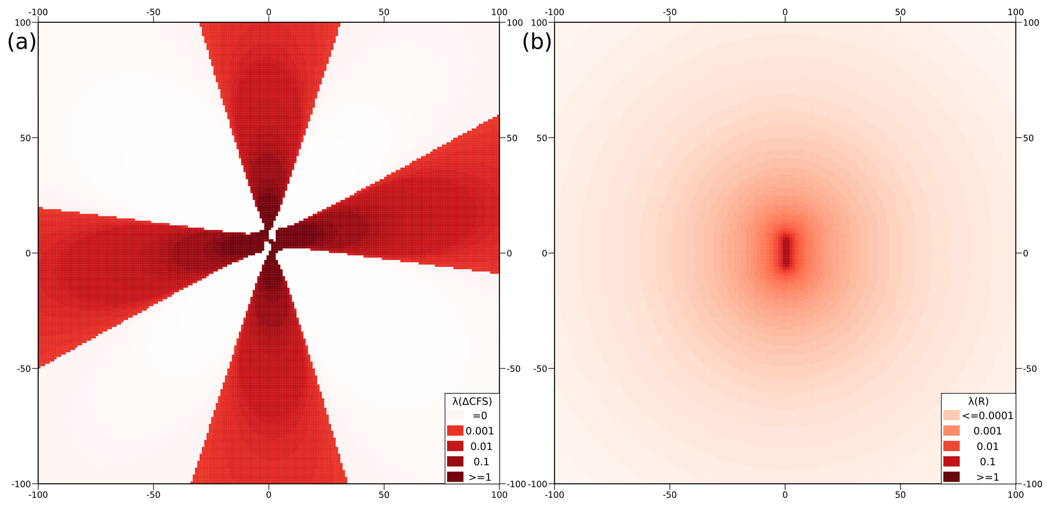
Figure 1 The forecast is created for the synthetic experiment to assess the usefulness of the receiver operating characteristic (ROC) curve in differentiating the two forecast models. (a) Coulomb forecast model, calculated for a spatial grid of 10×10 km at a depth of 7.5 km for the analysis. (b) A reference model with probability decaying as a function of distance ($c\cdot d^{-\mathrm{2}}$) from the fault plane.

We used the ΔCFS clock advance model to simulate synthetic aftershock distributions in response to positive and negative stress changes. We generated catalogs with up to N=500 synthetic aftershocks. In the first step, all generated aftershocks directly stem from the ΔCFS model, allowing earthquakes only to occur only in the regions with a positive stress change. The AUC of the ROC curves is then computed for both ΔCFS and R models. However, such a perfect combination of forecast and observation is not realistic because multiple factors can cause earthquakes in the negative stress regions, such as secondary stress changes due to afterslip or aftershocks (Cattania et al., 2014), the oversimplification of mainshock slip geometry (Hainzl et al., 2009) and dynamic triggering (Hardebeck and Harris, 2022), etc. Thus, we considered this mismatch by sampling one, two, and more events out of total aftershocks in the negative stress regions (referred to as shadow earthquakes – SEs) and repeated the computation of AUC for both forecast models.

3.1 Test using ROC

ΔCFS shows a slightly better AUC value than the R model in the case of perfect data. However, the AUC value for the ΔCFS model starts decreasing with adding earthquakes into the shadow regions due to increasing FNs, which eventually reduces TPR, leading to decreased AUC. ROC curves generated for single synthetic catalogs are shown in Fig. 2a, visualizing that there is no clear distinction between the performance of the ΔCFS (red curves) and R (blue curve) models if there is a slight imperfection in the ΔCFS forecast induced by SEs. To quantify the outcome of ROC, we repeated the same experiment 100 times for different synthetic catalogs and present the resulting distribution of AUC values in Fig. 2b. Ideally, there should be a clear separation between the AUC values of the (almost) true ΔCFS model and the rather uninformative R model. However, Fig. 2b shows that with three SEs in the observed catalogue, the distributions start to overlap and keep increasing with increasing SEs, showing that an uninformative forecast model can outperform a ΔCFS model unless the latter perfectly represents the data. This result is in accordance with the findings of Parsons (2020), highlighting the inability of the ROC to perform meaningful testing in this synthetic scenario. Furthermore, the ROC curve tends to provide an inflated overview of the performance for negatively imbalanced datasets because changes in the number of FP have little effect on FPR (Eq. 2).

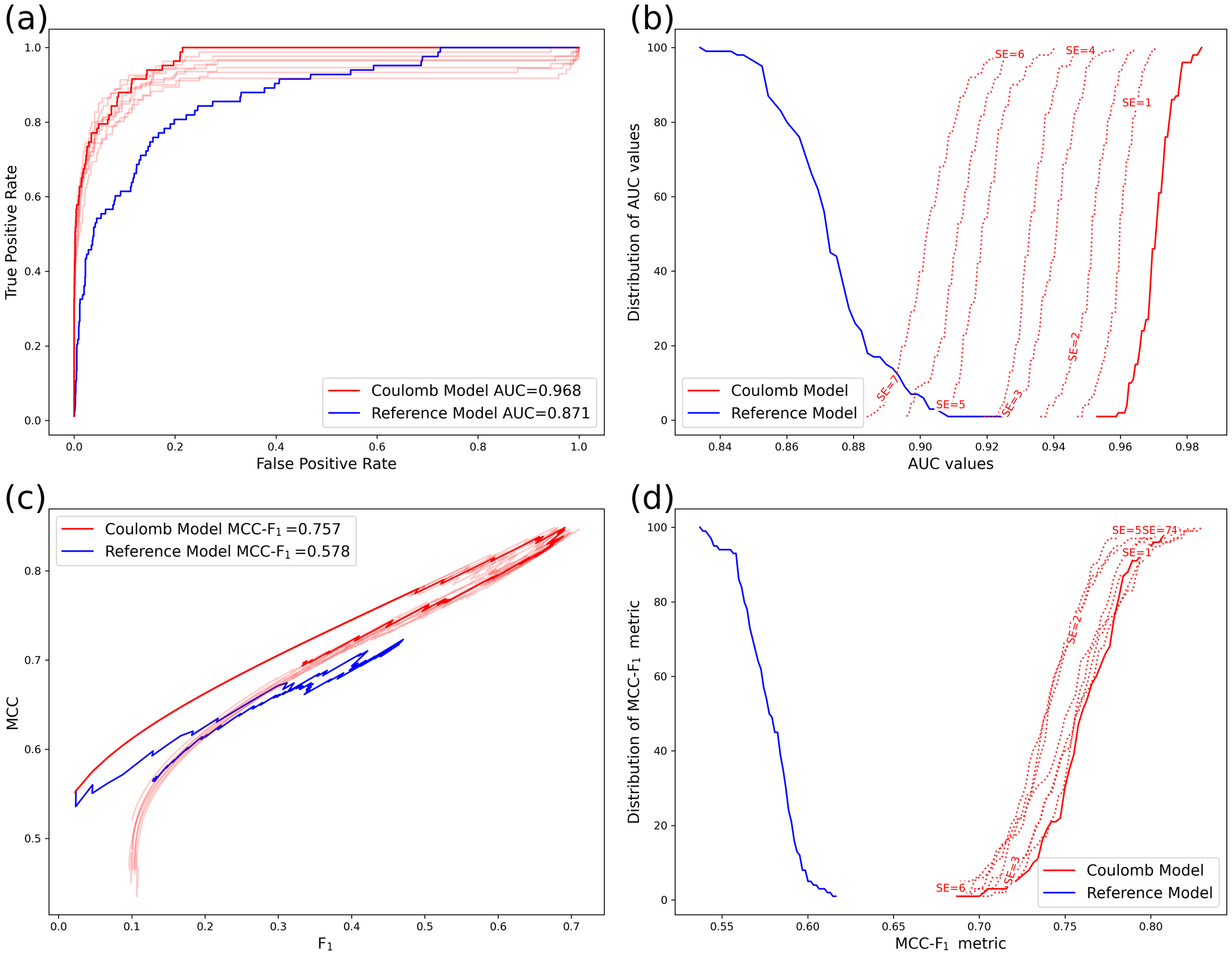
Figure 2 ROC and MCC-F1 curves calculated for the Coulomb model (ΔCFS) and the less informative reference model (R) against the same synthetic aftershock simulations. The solid red curves show the ΔCFS results for aftershocks in perfect agreement with the Coulomb model, while the dotted lines present cases with up to seven earthquakes, so-called shadow earthquakes (SEs), falling into cells with negative ΔCFS. The blue curve refers to the R model, where the aftershock probability is a simple function of the distance (d) from the mainshock hypocentre ($s_i=c{d}_i^{\mathrm{-}\mathrm{2}}$), where c is a constant. (a) Examples of ROC curves for a single distribution of aftershocks with up to seven SEs. (b) Distribution of AUC of the ROC values for 100 different aftershock simulations for each SE number. Note that the blue curve corresponds to the inverse cumulative distribution function of AUC for the R model, while the red curves refer to the cumulative distribution function of AUC for the Coulomb model. In this way, the separation between the corresponding distributions of the two models can be easily visualized. (c, d) Corresponding results for the MCC versus F1 curves and the MCC-F1 distributions.

3.2 Test using MCC-F₁

We repeated the analysis with the MCC-F₁ curve for the same experiment. Figure 2c visualizes the performance of the MCC-F₁ curve for the ΔCFS model (red) against the R model (blue), showing clear differentiation between the two forecasts. The performance of the ΔCFS model with introduced imperfections is also shown (dim red) for SEs 1 to 7. Visually, the MCC-F₁ curves are more distinct than the ROC curves. We repeated the experiment 100 times and quantified the performance of MCC-F₁ by showing the distribution of the MCC-F₁ metric in Fig. 2d. The figure shows that MCC-F₁ improved the testing capability in differentiating between the ΔCFS model and R forecast.

3.3 Test using a multi-resolution grid

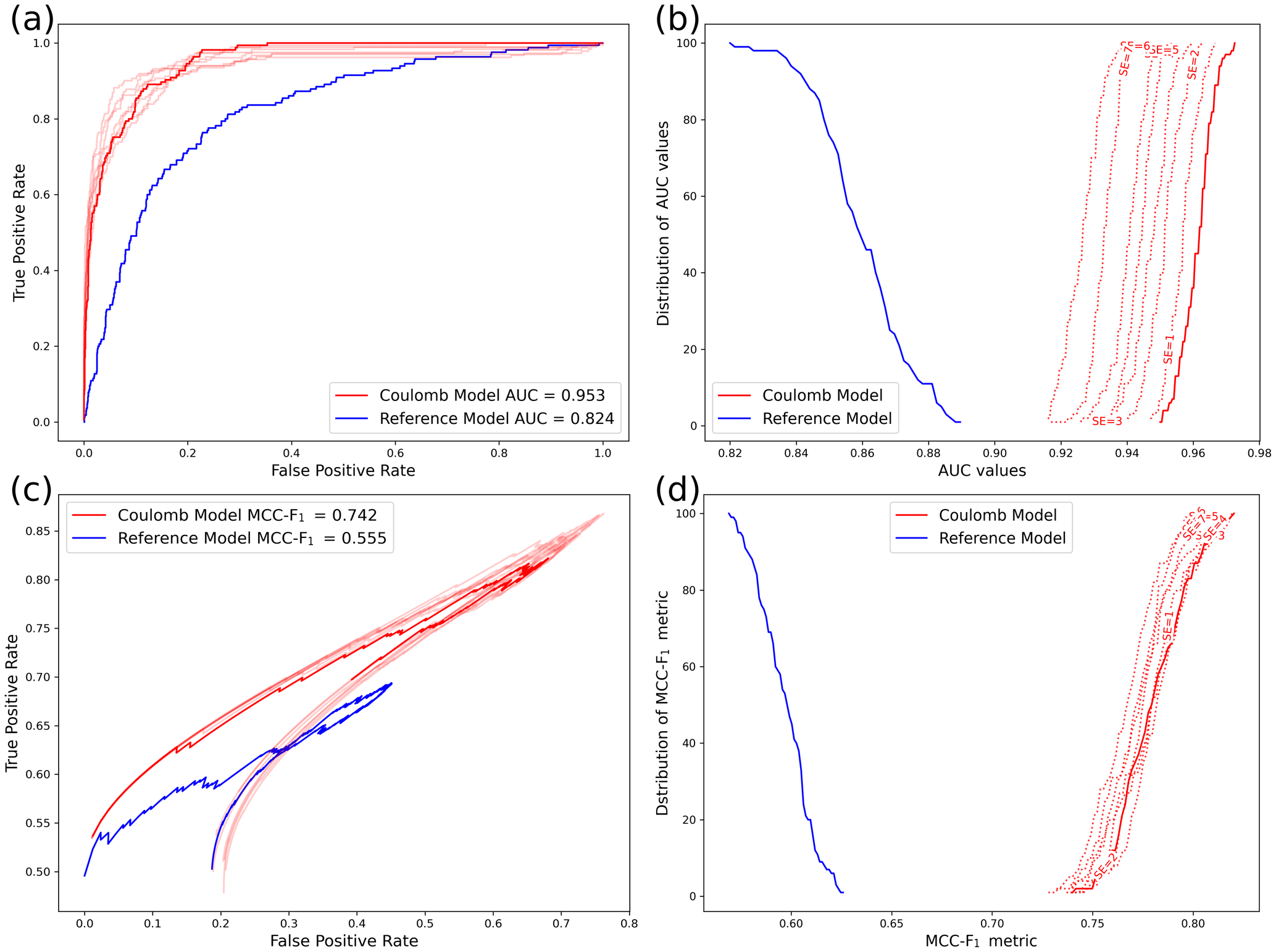
We repeated the experiment using a radial multi-resolution grid described in Sect. 2.2. In particular, we created a radial grid with the same number of spatial cells as the single-resolution grid, aggregated the ΔCFS and R forecasts on this grid, and repeated the synthetic experiment. Khawaja et al. (2023a) showed that a forecast can be aggregated on another grid without affecting its consistency. A sample radial grid is shown in Fig. S1. The corresponding results for both models using ROC and MCC-F₁ curves are visualized in Fig. 3a and c, respectively. Using a multi-resolution grid, both ROC and MCC-F₁ can provide distinctive curves for the ΔCFS and R forecasts with up to seven SEs. We repeated the forecast evaluation 100 times with different synthetic catalogs and show the distribution of the resulting AUC and MCC-F₁ values in Fig. 3b and d, respectively. ROC and MCC-F₁ can clearly differentiate between the ΔCFS and uninformative R forecasts when evaluated using a multi-resolution grid. The separation of the AUC and MCC-F₁ distributions is best for synthetics perfectly in line with ΔCFS. The separation is reduced by introducing imperfections in the ΔCFS model in the form of SEs. However, the range of the AUC and MCC-F₁ values remains distinct for both forecasts up to seven SEs, indicating that the multi-resolution grid has helped to improve the testability of the aftershock forecast models. We can also see that using MCC-F₁ in combination with a multi-resolution grid provides the most distinctive test results.

Figure 3 Same as Fig. 2 but for a radial test grid.

3.4 Recommendation for testing aftershock models

The usefulness of a testing metric has been discussed in the context of the quantity of the observed data in many studies for different fields of research (e.g. Bezeau and Graves, 2001; Kanyongo et al., 2007; Liew et al., 2009; Button et al., 2013; Mak et al., 2014; Sham and Purcell, 2014, etc). Particularly in the context of earthquake forecast evaluation, Khawaja et al. (2023a) proposed that reducing disparity in the number of spatial cells and the number of observations increases the statistical power of the tests. Keeping this in view, we used our experimental setup to provide a guideline about the minimum quantity of data required for meaningful evaluation of forecasts in terms of binary occurrences and non-occurrences. We used the ΔCFS model to simulate catalogs with different earthquake numbers but a fixed number of cells containing earthquakes (also referred to as active cells). In particular, we controlled the number of spatial cells that receive earthquakes by simulating one aftershock after the other on the same square grid with a total of 1600 cells until the desired number of cells receive earthquakes. This allows us to control the disparity in the testing. We repeated the experiment 100 times for every case, and results are recorded as a distribution of AUC value and MCC-F₁ metric. Since ΔCFS is a seismicity-generating model, it is a perfect model and should outperform the R model. To quantify the separation between the ΔCFS and the R distributions, we calculated the difference between the 1 % quantile of the ΔCFS values and the 99 % quantile of the R values, i.e. $\mathrm{\Delta }=\mathrm{\Delta }{\mathrm{CFS}}^{\mathrm{1}\mathit{\%}}-{\mathrm{R}}^{\mathrm{99}\mathit{\%}}$. Both distributions are significantly separated if Δ>0. We repeated this calculation for different numbers of active cells. Figure 4 shows the result as a function of the percentage of active cells, i.e. cells with at least one earthquake. The figure shows that if we compare a perfect forecast model with an uninformative model, we should have at least 3 % of active cells for differentiating the two forecast models in terms of ROC and MCC-F₁. The imbalanced data with a class ratio of more than 97:3 in favour of the negative class does not ensure accurate testing, even if one model is perfect and the other is uninformative.

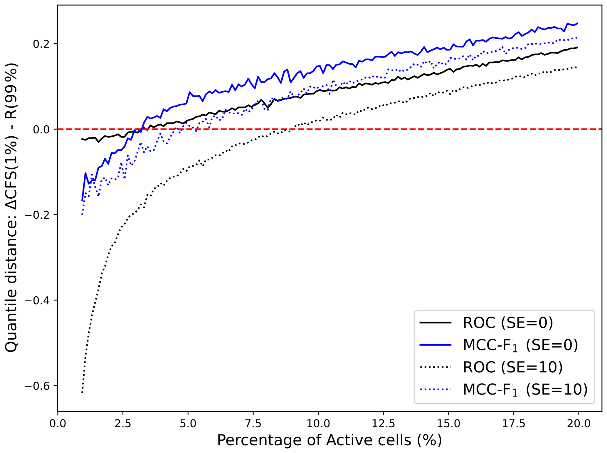
Figure 4 Separation of the distributions of the ΔCFS and R model as a function of the number of cells containing observed earthquakes, measured by the difference between the 1 % quantile of ΔCFS and the 99 % quantile of the R model. Both distributions overlap for negative values (below the horizontal dashed line). Thus, the values need to be above this line for meaningful testing.

In reality, there is no perfect forecast model available. To address this, we repeated the experiment with added imperfections by randomly adding earthquakes in 10 cells with negative stress changes. In this case, our analysis shows that one needs approximately 5 % and 8 % active cells to differentiate between the two models using MCC-F₁ and ROC, respectively. These values represent a minimum test requirement that should be met for meaningful testing of earthquake forecast models for observed data using the discussed binary testing metrics. Because we cannot control the number of observed earthquakes, we can only ensure this requirement by adapting multi-resolution grids accordingly.

4 Real case studies

After highlighting the importance of using multi-resolution grids for testing the aftershock models using a simple radial grid based on a synthetic experiment, we evaluated the aftershock models for real aftershocks of the 1999 Chi-Chi and 1992 Landers earthquakes. In this case, we used the Quadtree approach to create spatial grids for representing the earthquake forecast models.

We generated three single-resolution grids and one multi-resolution grid around the mainshock region within a distance of 100 km from the fault. The three single-resolution grids are zoom level 14 (L14), zoom level 13 (L13), and zoom level 12 (L12). Grid L12 contains the least number of bigger cells, L13 has 4 times more cells of half dimension, and L14 has 16 times more cells with quartered dimensions. However, we trimmed those cells along the boundary that falls outside of 100 km. To consider the testing in a 3D-space, we considered depth bins of 2, 4, and 8 km for L14, L13, and L12, respectively. For creating the multi-resolution grid, we keep the resolution to L14 within 10 km of the fault zone, L13 from the radius of 10 to 60 km, and L14 outside 60 km, along with their respective depth bins.

We used variable slip models for 1999 Chi-Chi (Ma et al., 2000), and 1992 Landers (Wald and Heaton, 1994) earthquakes provided in the SRCMOD database (http://equake-rc.info/srcmod/, last access: December 2022) maintained by Mai and Thingbaijam (2014). We added the 1992 Big Bear earthquake slip (Jones and Hough, 1995) to the Landers slip model. For each slip model, we calculated the static stress tensor on the grid points of our target region (up to 100 km from the mainshock rupture plane). For this purpose, we again used the PSGRN + PSCMP tool (Wang et al., 2006) to calculate the coseismic stress changes in a layered half space based on the CRUST 2.0 velocity model (Bassin, 2000).

The aftershock models for both earthquakes are aggregated on the four 3D grids. We calculated the ΔCFS model for receiver mechanisms identical to the mainshock mechanism, namely strike = 5^∘ (330^∘), dip = 30^∘ (89^∘), and rake = 55^∘ (180^∘) for Chi-Chi (Landers). To visualize, the forecast for 3D cells around 7.5 km is displayed after normalizing by the cell volume in Figs. 5 and 6 for Chi-Chi and Landers, respectively. The non-normalized ΔCFS models for Chi-Chi and Landers are provided in Figs. S2 and S3, respectively.

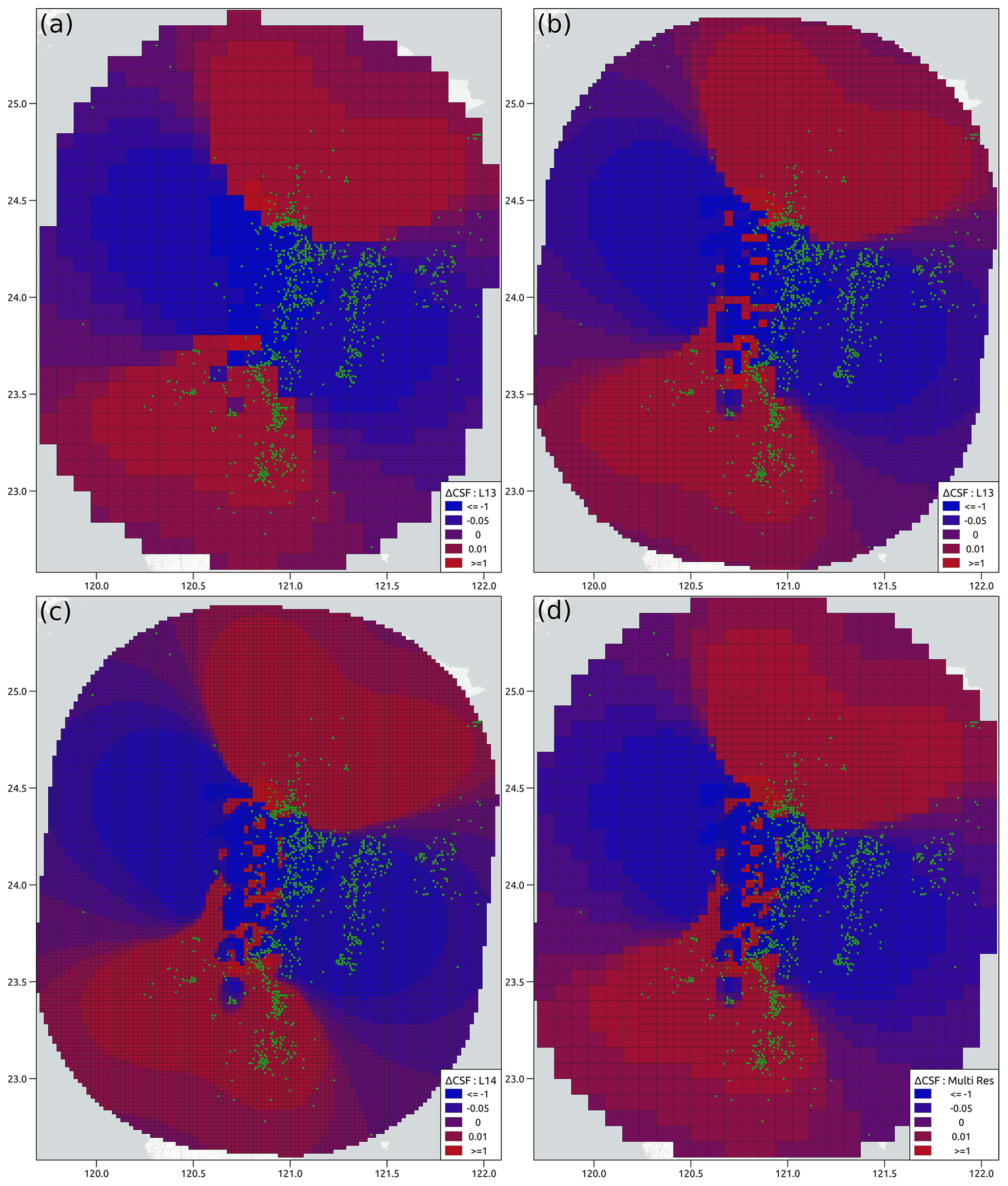
Figure 5 Colour-coded Coulomb stress changes (in units of MPa) for the Chi-Chi earthquake along the master fault aggregated on 3D grids of (a) L12, (b) L13, (c) L14, and (d) multi-resolution grid.

In both cases, we selected earthquakes that occurred within the 1 year after the mainshock with horizontal distances of less than 100 km to the mainshock fault. For the Chi-Chi earthquake, we used the International Seismological Centre (ISC) catalogue. The aftershock data for Landers are acquired from the Southern California Earthquake Data Center (SCEDC) (Hauksson et al., 2012). To account for the general catalogue incompleteness, we used a magnitude cutoff of M_c=2.0 for Landers (Hutton et al., 2010) and M_c=3.0 for Chi-Chi. The number of aftershocks that participated in the evaluation for the gridded forecasts is 2944 for Chi-Chi with a depth range of up to 48 km, while it is 13 907 for Landers with a depth range of up to 32 km.

For Chi-Chi, the percentage of active cells (positive class) is 0.75 %, 3.8 %, 12 %, and 5 % for grids L12, L13, L14, and multi-resolution, respectively. Similarly, for Landers, we have 1.2 %, 4 %, 12.8 %, and 10.3 % cells with earthquakes for grids L12, L13, L14, and multi-resolution, respectively. We can see that uniformly reducing the resolution can reduce the imbalanced nature of data. For the L12 grid, the minimum percentage of active cells is achieved, according to our analysis in Sect. 3.4. However, with uniformly decreasing the resolution, we may lose important information near the fault plane. Thus, a multi-resolution grid, also fulfilling the requirement, can be considered a better trade-off between the details provided by the model and less imbalanced data.

As can be seen in Fig. 5, numerous aftershocks of the Chi-Chi earthquake occurred in the negative stress regions of the CF model; therefore, ΔCFS is not supposed to perform well. Sharma et al. (2020) reported the AUC = 0.476 for the CF model using 1-year aftershock data evaluated for a 5 km × 5 km gridded region around the Chi-Chi mainshock. Table 1 provides our results of the performance in terms of ROC and MCC-F₁ for Chi-Chi aftershock forecasts using the four different grids. The AUC values are in a similar range for the different Quadtree grids, i.e. AUC for L12, L13, L14, and multi-resolution is 0.452, 0.415, 0.394, and 0.437, respectively. The AUC for the R model is 0.705, 0.765, 0.794, and 0.768 using the L12, L13, L14, and multi-resolution grids. It shows that the relative ranking of the forecast models remains the same for different grids, which is not surprising given the fact that many observed earthquakes occurred in the negative stress regions of the Coulomb model. The MCC-F₁ metric for the L12, L13, L14, and multi-resolution grids is 0.367, 0.303, 0.253, and 0.261, respectively. The MCC-F₁ metric for the reference model is 0.486, 0.373, 0.288, and 0.366 for the L12, L13, L14, and multi-resolution grids. The relative ranking of the forecast models also remains the same based on the MCC-F₁ metric.

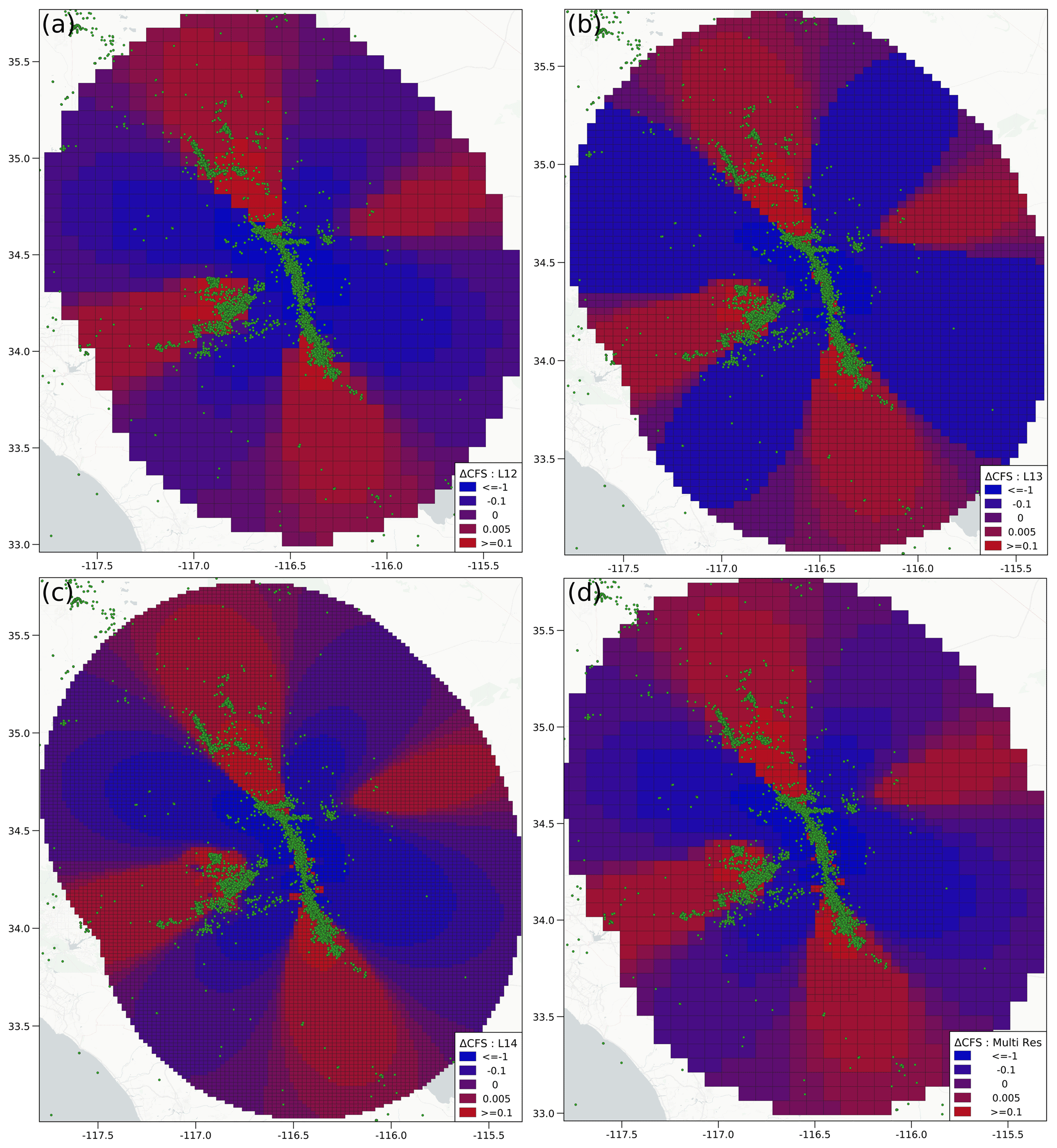
Figure 6 Coulomb stress changes (MPa) for the Landers earthquake along the master fault aggregated on 3D grids of (a) L12, (b) L13, (c) L14, and (d) multi-resolution grid.

Table 1 Evaluation of aftershock forecast models for the Chi-Chi and Landers earthquakes based on AUC values and MCC-F1 for four grid resolutions. The main ΔCFS result refers to stress changes calculated for the mainshock mechanisms, while the corresponding results for optimally oriented planes (OOPs) are provided in brackets.

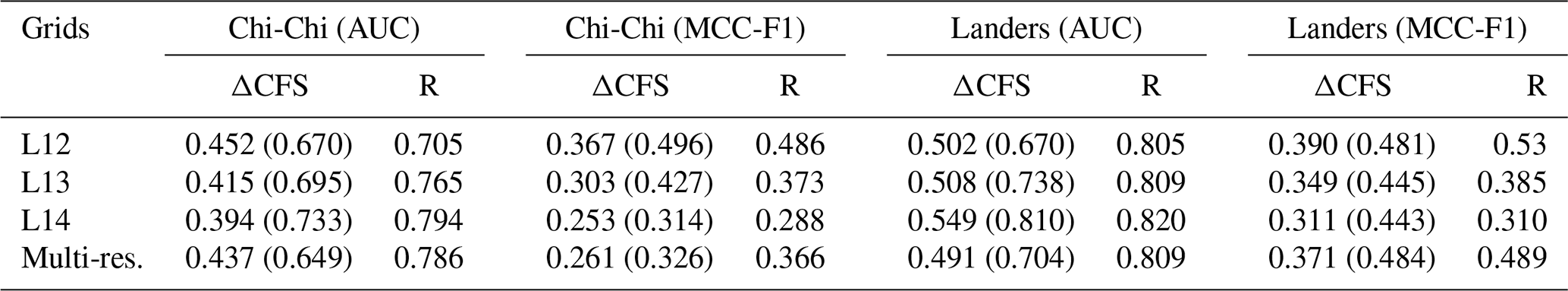
Figure 6a–d show that aftershocks also occurred in the negative stress regions of ΔCFS model in the Landers case. The performance in terms of ROC and MCC-F₁ for Landers aftershock forecasts is computed and provided in Table 1. The ΔCFS forecast model shows AUC values of 0.502, 0.508, 0.549, and 0.491 for grids L12, L13, L14, and multi-resolution. While the MCC-F₁ metric yielded values of 0.390, 0.349, 0.311, and 0.371 for the L12, L13, L14, and multi-resolution grids. The R model outperforms the ΔCFS model again.

One reason for the failure of the ΔCFS model could be our simplistic calculations of ΔCFS, assuming the same rupture mechanism for the mainshock and all aftershocks. However, variable aftershock mechanisms are usually observed. One way of dealing with this is to calculate the Coulomb stress on optimally oriented planes (OOPs), which maximize the total stress consisting of the background stress field and the mainshock-induced stresses. Thus, we have repeated the analysis also for OOPs, assuming a background stress field with its orientation and strength. Here, we set the orientation of the principal stress components so that the mainshock was optimally oriented to the background stress field. Furthermore, we use a differential stress of 3 MPa (σ₁=1, σ₂=0, and σ₃=−2 MPa), which agrees with the average stress drop of interplate earthquakes (Allmann and Shearer, 2009). The corresponding results are provided in Table 1 (in brackets), showing similar outcomes, indicating that the ΔCFS model is not better than the R model for the Chi-Chi, but it is comparable with the R model for the Landers aftershock forecast.

Thus, changing grids does not particularly favour the ΔCFS forecast model, and we are confident that the forecast evaluation, in these cases, is not particularly affected by the imbalanced nature of the dataset as feared in most evaluations based on ROC for highly imbalanced datasets. For improvements, the basic ΔCFS forecast model needs to be based on more sophisticated approaches, such as considering, for example, secondary triggering, fault structure, seismic velocity, and heat flow. (Cattania et al., 2014; Asayesh et al., 2022, 2020a; Hardebeck, 2022). In the future, we intend to conduct a thorough re-evaluation of models based on different stress scalars (Sharma et al., 2020), after improving the imbalanced nature of the test data by harnessing the convenience of multi-resolution grids following the guidelines of this study.

5 Conclusions

Coulomb stress changes (ΔCFS) are computed for a gridded region by taking into account the complexities of a fault in the aftermath of a mainshock to determine the regions with increased or decreased seismicity. The aftershock forecasts are evaluated using the ROC curve, and many studies show that ΔCFS is under performing. However, it is also known that ROC is not effective for evaluating the datasets where the negative class is in higher proportion compared to the other. In this context, we conducted a synthetic experiment to understand the usefulness of the ROC and find its weakness in differentiating between a perfect forecast and an uninformative forecast. We proposed using the Matthews correlation coefficient (MCC) and F₁ curve instead of ROC to evaluate the forecast models and found it to be better in distinguishing between the two models using the same experiment. We further explored that the quantity of observed earthquakes affects the capability of the test. Our analysis shows that at least 5 % and 8 % of cells need to have recorded earthquakes to meaningfully evaluate the forecast models using MCC-F₁ and ROC, respectively. The lower threshold for MCC-F₁ again proves the superiority of MCC-F₁ over ROC. Since we cannot control the observed data, we should adjust the spatial grid representing the forecast models according to the data to reduce the disparity in the data. We also demonstrate the use of the Quadtree approach to generate data-driven multi-resolution grids to evaluate the aftershock forecasts for earthquakes of Chi-Chi and Landers following the suggested guidelines. The outcome of evaluating these aftershock forecasts suggests that changing of the spatial grid for testing does not favour the outcomes of the test in the favour of any model; rather, reducing disparity makes the testing outcome more reliable.