Semi-automatic mapping of shallow landslides using free Sentinel-2 images and Google Earth Engine

The global availability of Sentinel-2 data and the widespread coverage of cost-free and high-resolution images nowadays give opportunities to map, at a low cost, shallow landslides triggered by extreme events (e.g. rainfall, earthquakes). Rapid and low-cost shallow landslide mapping could improve damage estimations, susceptibility models and land management.

This work presents a two-phase procedure to detect and map shallow landslides. The first is a semi-automatic methodology allowing for mapping potential shallow landslides (PLs) using Sentinel-2 images. The PL aims to detect the most affected areas and to focus on them an high-resolution mapping and further investigations. We create a GIS-based and user-friendly methodology to extract PL based on pre- and post-event normalised difference vegetation index (NDVI) variation and geomorphological filtering. In the second phase, the semi-automatic inventory was compared with a benchmark landslide inventory drawn on high-resolution images. We also used Google Earth Engine scripts to extract the NDVI time series and to make a multi-temporal analysis.

We apply this procedure to two study areas in NW Italy, hit in 2016 and 2019 by extreme rainfall events. The results show that the semi-automatic mapping based on Sentinel-2 allows for detecting the majority of shallow landslides larger than satellite ground pixel (100 m²). PL density and distribution match well with the benchmark. However, the false positives (30 % to 50 % of cases) are challenging to filter, especially when they correspond to riverbank erosions or cultivated land.

1 Introduction

One of the recent and forecasted impacts of climate change is the rise of extreme meteorological events (IPCC, 2014). During extreme rainfall, one of the most common phenomena is the activation of shallow landslides (Gariano and Guzzetti, 2016; Guzzetti et al., 2004) as defined by Guzzetti et al. (2006) and Caine (1980). Shallow landslides are triggered not only by rainfall but also by other extreme events like earthquakes (Sassa et al., 1996) or rapid snow melting (Cardinali et al., 2000). These slope instabilities usually involve soils and superficial deposits and represent a meaningful impact on infrastructures (e.g. road networks) and cultivated areas. The pervasive distribution of these phenomena on slopes, hereafter called extreme events, makes their identification and mapping crucial for effective damage evaluation. For this reason, the definition of procedures and strategies aimed at mapping shallow landslides has deeply been investigated in the last few decades to reach different final goals like (i) the mapping of the full extent of a landslide disaster (Guzzetti et al., 2004), (ii) the study of geomorphological and erosion phenomena (Fiorucci et al., 2011), (iii) the validation of susceptibility models (Bordoni et al., 2015; Cignetti et al., 2019; Rossi et al., 2010), and (iv) the statistical comparison of landslide inventories from different methodologies and sensors (Carrara, 1993; Fiorucci et al., 2018).

Landslide event inventory maps are commonly implemented using several different methodologies: (i) post-event aerial photo analysis and plotting (Cardinali et al., 2000), (ii) manual or automatic identification based on the use of high-resolution digital elevation models (DEMs) obtained from airborne lidar surveys done after the event (D'Amato Avanzi et al., 2015; Giordan et al., 2017), and (iii) traditional geomorphological field surveys (Pepe et al., 2019). In recent years, even satellite images have been used to identify and map shallow landslides (Ghorbanzadeh et al., 2021; Lu et al., 2019; Martha et al., 2010; Mondini et al., 2011; Qin et al., 2018). This recent evolution has been possible thanks to the robust improvement of satellite resolution (sub-metric for most commercial satellites), which nowadays is not so different from aerial images (Fiorucci et al., 2019). Recent studies have mostly been based on commercial high-resolution satellite images. The use of these commercial images often requires committed acquisition planning after the event that results in a high cost and limits the use of these systems. For instance, areas with a low human or infrastructure presence are often overlooked by authorities that mainly dedicate funds to study more inhabited sectors. The scarcity of resources creates a bias between high-income populated areas and remote areas or developing countries that cannot afford the cost.

In the last few years, the Sentinel satellite constellation of the Copernicus programme made medium–high-resolution images, (about 10 m) both multi-spectral (Sentinel-2) and SAR (Sentinel-1), available free of cost and with a high-frequency revisit rate.

In addition, several areas of the world are covered by multi-temporal very-high-resolution images of Google Earth™ that could help to detect and map shallow landslides when pre- and post-event images are available (Borrelli et al., 2015). Google Earth Engine (GEE) cloud processing (Gorelick et al., 2017) could also be used to create time series of several satellite data (optical, SAR), which are useful to detect the change in and the recovery of vegetation and to map landslides and their effect on vegetated areas (Scheip and Wegmann, 2021; Yu et al., 2018; Handwerger et al., 2022; Lindsay et al., 2022; Ganerød et al., 2023).

In this study, we utilised pre- and post-event normalised difference vegetation index (NDVI) data from Sentinel-2 to develop a dedicated methodology for semi-automatically detecting potential shallow landslides. To assess the accuracy of our approach, we compared the potential landslides detected using our method with a benchmark inventory manually mapped on post-event high-resolution images.

We utilised the Google Earth Engine (GEE) platform to generate the NDVI time series, which allowed us to pinpoint the optimal image pairing for detecting potential landslides, calculate multi-temporal NDVI averages and keep track of vegetation regrowth in the impacted regions.

Our methodology aims to provide a more user-friendly approach compared to similar studies. We achieved this by using cost-free data, open-source software and empirical thresholding, which makes it easier to replicate our approach in other regions affected by shallow landslides. The implemented methodology has been tested in two areas of north-western Italy hit by extreme rainfall events in recent years, i.e. November 2016 and October 2019. The two events triggered hundreds of shallow landslides in small areas, causing widespread damage to the road network; cultivation; and, in some cases, urban areas.

Semi-automatic and manual inventories and GEE scripts have also been published online and are open for improvement by the scientific and user community.

2 Study areas

The two presented case studies are located in NW Italy, respectively, and were affected by two heavy rainfall events in November 2016 and October 2019.

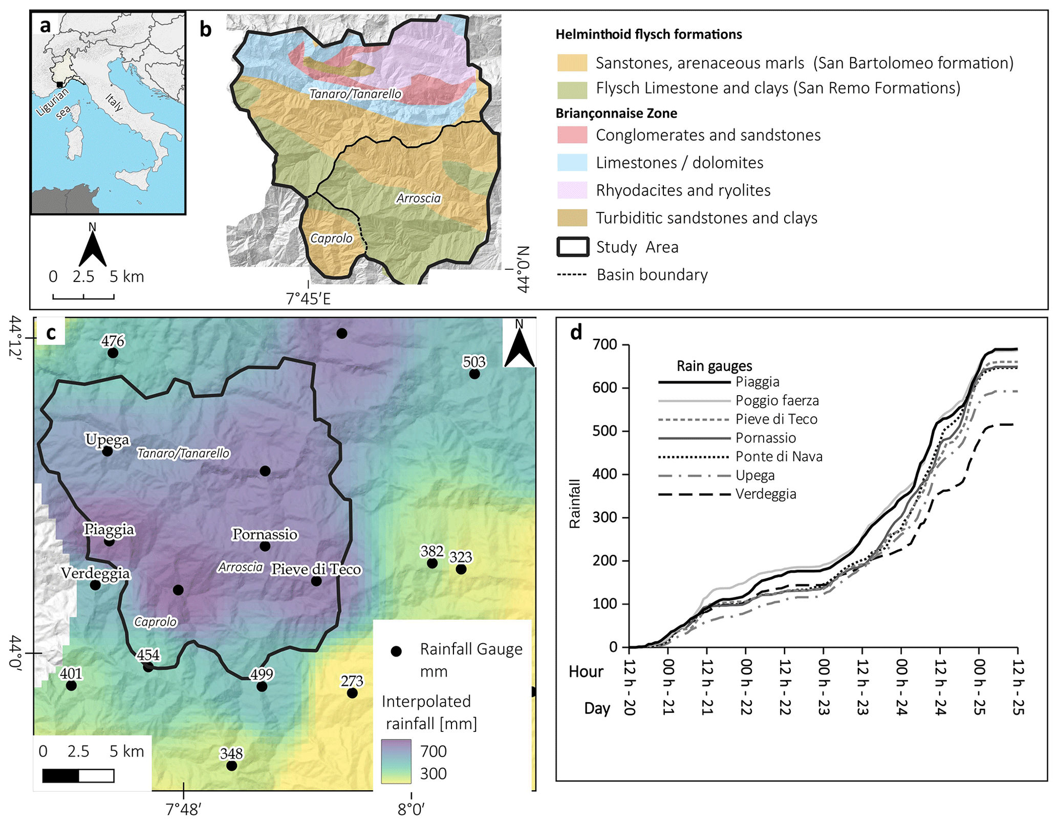
Figure 1 The Arroscia–Tanarello November 2016 event. (a) Location of the study area, (b) simplified geological map based on Lanteaume et al. (1990) and (c) accumulated rainfall from 20 to 25 November 2016 in the study area. (d) Hourly cumulated rainfall for some rain gauge stations of study areas. Rainfall source: ARPA (Agenzia Regionale Protezione Ambiente) Piemonte and ARPAL (Agenzia Regionale Protezione Ambiente Liguria). Shaded reliefs of maps in panels (b) and (c) are based on the DTM of ARPA Piemonte and Liguria.

The 2016 event area (about 350 km²) is located in the Ligurian Alps at the border between the Liguria and Piemonte regions (NW Italy). The shape and the extension of the study area (Fig. 1) are a combination of (i) the area most severely hit by rainfall, (ii) other literature studies of the event (Cremonini and Tiranti, 2018; Pepe et al., 2019), and (iii) the footprint of the available Sentinel-2 cloud-free images and the post-event Google Earth images. The area of interest (AOI), henceforth called the Tanarello and Arroscia valleys, shows an elevation up to 2500 m a.s.l. and a wide range of land use and vegetation cover from the Mediterranean to the alpine environment. The area intersects several river basins, and the main catchments are the Tanaro–Tanerello, a part of the Po River basin and the Arroscia stream flowing to the Ligurian Sea. From a geological point of view (Fig. 1b), the northern sector of the area is occupied by the Briançonnaise Zone of the middle Pennidic nappe. This unit is represented by limestone–dolomite, which creates steep slopes, as well as conglomerate and volcanic formations (rhyolite). In the southern part of the area is an outcropping of the Helminthoid Flysch formations of Monte Saccarello–San Remo, made by a limestone–clay sequence, and the sandstone–siltstone sequence of the San Bartolomeo Formation (Lanteaume et al., 1990; Pepe et al., 2015). The Tanarello and Arroscia Valley area has a sparse human settlement and low population density, ranging from 40 to 1 inhabitant per square kilometre. Most of the inhabitants live in Ormea and Pieve di Teco. Most of the area is occupied by broadleaf forests in the lower part and coniferous forest, grassland and pasture at high altitudes.

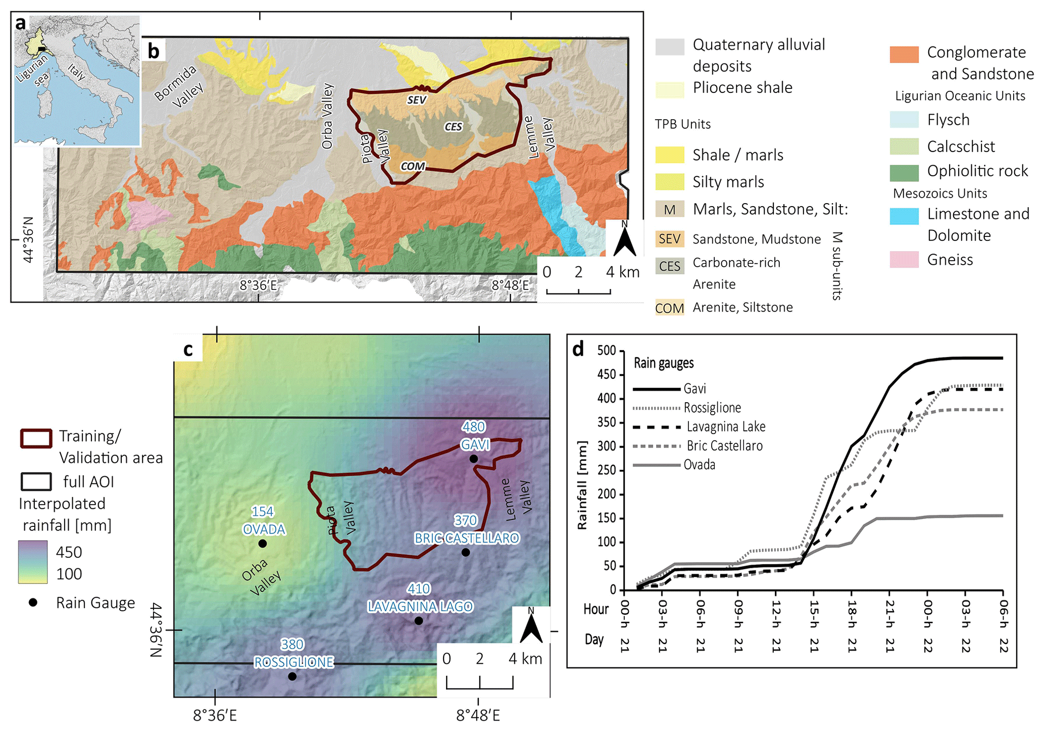
Figure 2 The Gavi October 2019 event. (a) Location of the study area, (b) simplified lithological map of the study area based on Piana et al. (2017) and (c) accumulated rainfall from the 21 to 22 October 2019 event. (d) Hourly cumulated rainfall for some rain gauge stations of study areas. (Rainfall data source: ARPA Piemonte). Shaded reliefs of maps in panels (b) and (c) are based on the DTM of ARPA Piemonte and Liguria.

The area affected by the heavy rainfall event in 2019 (about 530 km²) is located between the Bormida River and Lemme valleys, in the south-eastern Piemonte region. The considered area has been delimited considering the effects of the event based on the rainfall data, image coverage and reports on damages. The study area mostly overlaps with the Tertiary Piedmont Basin (TPB): a sedimentary succession from Oligocene conglomerates in the south to Pliocene mudstone in the northern part (Fig. 2b). Three main geological formations outcrop in the detailed training areas, from south to north: the Cortemillia Formation (made by arenite and mudstone), the Cessole Marls (made by carbonate-rich mudstone and arenite) and the Serravalle Formation (made by arenite and sandstone). The southern part is occupied by ophiolitic rocks of the Ligurian oceanic unit (Piana et al., 2017). Alluvial quaternary deposits occupy the bottom of the valley. Several small creeks cross the study area with S–N directions that, in the 2019 event, caused flash floods (Mandarino et al., 2021). The presence of a gentle hilly landscape characterises the geomorphology of the area. However, the slope is steeper in the northern sector than in the rest of the training area, where the Serravalle Formation outcrops. The vineyards (region of the Gavi grape) are mainly located in the central and southern parts of the study area (Cessole Marl formations). In contrast, the north-western part is mainly covered by broadleaf forest, sclerophyllous vegetation and shrubs. Several villages and the small town of Gavi are located inside the AOI, henceforth called the Gavi area. Shallow landslides frequently hit the castle of Gavi hill, such as during the 2014, 1977 and 1935 events (Govi, 1978; Mandarino et al., 2021).

From a climatological point of view (Fratianni and Acquaotta, 2017), Tanarello–Arroscia is between the Alpine and Ligurian–Tyrrhenian climate area, while the Gavi area is between Po Plain and the upper Adriatic region as well as the Alpine and Ligurian–Tyrrhenian zones. Moreover, the area of Gavi is also close to the area with a high frequency of intense rainfall (Fratianni and Acquaotta, 2017) in the NE sector of Liguria.

Recently, global warming and the related sea temperature increase likely caused a positive trend of extreme rainfall events in the area of the Ligurian Sea, especially on a short time interval (i.e. < 24 h) (Gallus et al., 2018; Paliaga and Parodi, 2022; Roccati et al., 2020).

2.1 The 20–25 November 2016 event in the Tanarello and Arroscia valleys

Historical information tells us that the Liguria region and NW Alps have usually been affected by several extreme rainfall events, usually during autumn (D'Amato Avanzi et al., 2015; Cevasco et al., 2014; Ferrari et al., 2021; Roccati et al., 2018; Guzzetti et al., 2004; Luino, 1999). From 20 to 25 November 2016, a low-pressure area affected the western Mediterranean Sea (Nimbus Web Eventi Meteorologici, 2022), causing heavy and persistent rainfall that hit NW Italy, and with high severity the Ligurian Alps. The upper valleys of the Tanarello and Arroscia streams (at the border between the Liguria and Piemonte regions) were the most severely hit by this event, and the rainfall accumulation reached 650–700 mm (Fig. 1c). The rain gauge station of Piaggia reached a value of 690 mm over 5 d, which is far higher than previous extreme events of the last 70 years (Fig. 1d). The dense network of rainfall gauges of ARPA Piemonte and ARPA Liguria (the regional agencies for environmental protection) allowed us to create a 1 km spatial resolution map of accumulated rainfall and compare precipitation time series for some stations. This heavy rainfall triggered many shallow landslides partly mapped with field surveys in Arroscia Valley (Pepe et al., 2019). Also, deeper landslides were triggered, like in the case of the village Monesi di Mendatica, which was partly destroyed by such a kind of landslide (ARPA Piemonte, 2018; Notti et al., 2021). Despite the limited human presence, the damages are estimated to be several millions of Euros for public infrastructures only.

2.2 The 21–22 October 2019 event in the Gavi area

The October to December 2019 period has been characterised by numerous meteorological events that hit NW Italy, causing an extremely rainy period (Copernicus Climate Change Service, 2019). In particular, on 19–21 October 2019, an extreme rainfall event hit the area between the Liguria and Piemonte regions, causing severe floods and diffuse shallow landslides in the basins of the Orba and Bormida rivers (Mandarino et al., 2021). This event was caused by a semi-stationary V-shaped storm over a relatively small area with extreme rainfall (Fig. 2c) both in hourly intensity and in total accumulation (Mercalli, 2019). This event activated many shallow and deep landslides. In particular, we focused on the area near the town of Gavi where the rain gauge registered about 480 mm per 24 h, and most of the rainfall (318 mm) was concentrated in 6 h intervals (Fig. 2d) (Meteologix, 2022). It is one of the highest rainfall records in the Piemonte region; just 5 years before (October 2014), extreme rainfall hit the same area. The extreme rainfall events of autumn 2019 caused estimated damages of EUR 16 million in the province of Alessandria (Regione Piemonte, 2021). After the October 2019 event, a particularly wet period triggered other shallow landslides in the study area until December 2019.

3 Materials and methods

One of the main effects caused by the activation of shallow landslides is the reduction in vegetation cover that creates a radiometric signature variation often detected by multi-spectral satellites. Thus, the NDVI is one of the most used band indexes to detect these variations (Fiorucci et al., 2019; Lu et al., 2019; Mondini et al., 2011). For this reason, we create a semi-automatic methodology that deals with pre- and post-event NDVI variation based on free satellite images with the best spatial resolution (Sentinel-2, nowadays).

Figure 3 Flowchart of proposed shallow landslide mapping methodology.

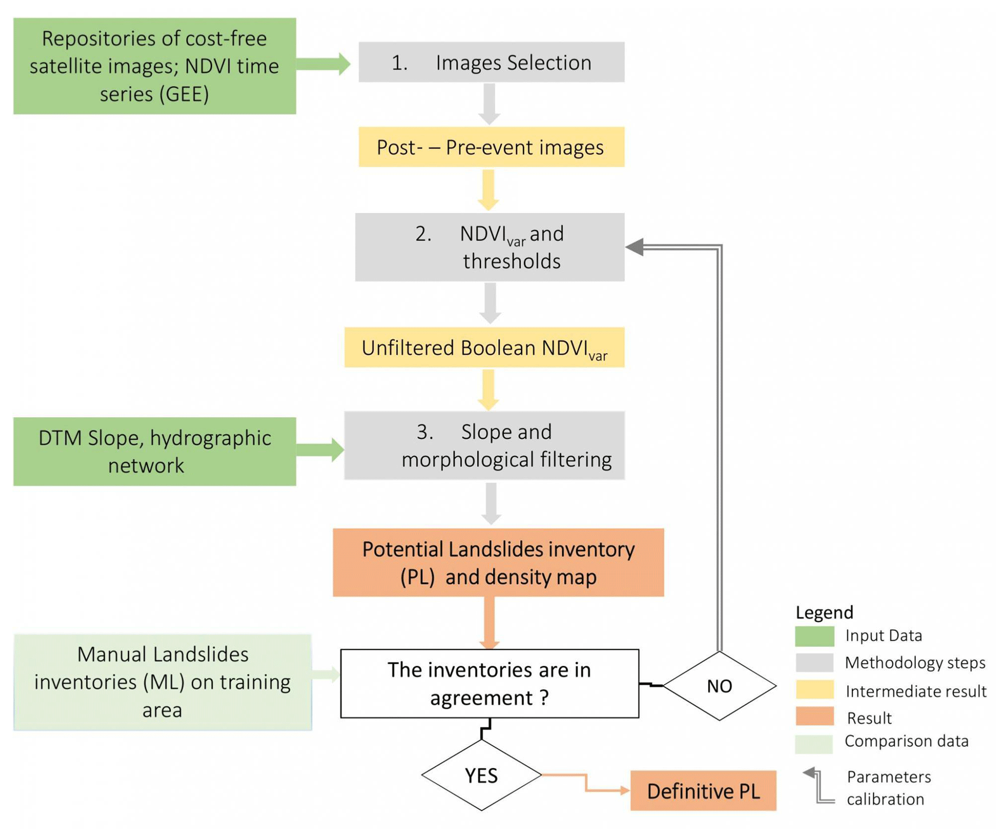
Our methodology, resumed in Fig. 3, aims to produce an inventory of potential shallow landslides (PLs) based on NDVI and geomorphological filters. The proposed method has two main phases: (i) in the first one, a semi-automatic methodology, divided into three main steps, identifies the potential high-density shallow landslide areas; (ii) in the second phase the semi-automatic inventory will further be used to support the manual mapping of landslides on very-high-resolution images. Time series of NDVI computed on GEE were also used to evaluate the vegetation recovery.

3.1 Potential landslide detection methodology

The proposed methodology (Fig. 3) is aimed at creating a PL inventory based on the semi-automatic procedure. The mapping method is based on the availability of pre- and post-event moderate-resolution (10 m) satellite images. This methodology is intended to detect surface changes, which are signs of potential shallow landslides, between pre- and post-event images. The PL inventory is aimed at delimiting the area most affected by shallow landslides and supports a subsequent detailed landslide mapping on very-high-resolution (< 1 m) images (satellite or aerial based). The PL is not a geomorphological landslide inventory because the shape of PLs is extracted with a semi-automatic procedure and is based on middle-resolution images. The PL inventory is created in three main steps: (i) satellite image selection, (ii) the calculation of the normalised difference vegetation index variation (NDVI_var) and the definition of the empirical NDVI_var threshold that is adopted for the potential landslide mapping, and (iii) the implementation of a filter using terrain and other geomorphological properties to obtain the potential shallow landslide (PL) inventory and the PL density maps. Thus, the PL inventory is compared over a training area covered by high-resolution images with a manually drawn dataset, i.e. manual landslides (MLs). This comparison phase is important because it is used for checking the efficiency of the PL methodology and refining the calibration of adopted parameters with iteration processes to improve the quality of the final PL inventory, reducing errors. The proposed methodology is exclusively based on cost-free software (e.g. QGIS, QGIS Association, 2022; SAGA GIS, Conrad et al., 2015; R, R Core Team, 2020) and cloud computing (e.g. GEE). In the following sections, the procedure is discussed in more detail.

3.1.1 Satellite image selection

The first step is the selection of the best pairs of pre- and post-event satellite images aimed at making a change detection analysis. Nowadays, the free satellite images with the best resolution are Sentinel-2 (10 m visible and near-infrared bands) followed by Landsat ones (30 m).

We search for images and filter images using the following criteria:

• i.

  cloud cover < 5 %;

• ii.

  images acquired in the same period of the year to minimise the effect of shadow and canopy cover changes related to different seasons;

• iii.

  the season with the highest NDVI to obtain a strong contrast in NDVI, no snow coverage, and a short shadow. The constraint period depends on local climatological conditions (e.g. summer from June to September in the middle latitude of the N Hemisphere).

To improve the search for the best pair of images, we also used output from a GEE processing based on the code developed by Nowak et al. (2021). The processing calculates a temporally averaged NDVI time series from a satellite image collection (e.g. Sentinel-2) filtered by cloud cover (< 5 %, or less if possible) over selected sample polygons that can directly be drawn on the satellite map interface of GEE. The time series plotted in a GEE chart can be exported to a CSV file for further filtering (e.g. replicate date removal) and analysis. We obtained a limited number of pairs of pre- and post-event images with these constraints.

3.1.2 NDVI_var calculation and threshold

In the second step, we calculated NDVI_var by computing the NDVI variation between the pre- and post-event conditions (Eq. 1). The aim is to identify areas with decreased NDVI values due to vegetation removal or damage caused by shallow landslides. Using the raster calculator of QGIS software, we computed the NDVI using the NIR and red band.

In the specific case of our study areas, we use the Sentinel-2 band of NIR (Band 8) and red (Band 4), which have a spatial resolution of 10 m:

$$\begin{array}{}\text{(1)}& {\mathrm{NDVI}}_{\mathrm{var}}={\mathrm{NDVI}}_{\mathrm{post}}-{\mathrm{NDVI}}_{\mathrm{pre}},\end{array}$$

where

$$\mathrm{NDVI}=(\mathrm{NIR}-\mathrm{Red})/(\mathrm{NIR}+\mathrm{Red}).$$

Then we manually select the NDVI_var threshold that best identifies changes related to landslides. This threshold does not have a fixed value, as reported in the literature (Hölbling et al., 2015; Mondini et al., 2011). An operator manually determines it after a visual assessment of NDVI_var, the comparison on GEE of the NDVI times series between affected and not affected areas, and the calibration of the parameters based on a PL–ML inventory comparison (back analysis). For instance, in our study areas, both the visual pattern of NDVI_var and the observation of the NDVI time series suggest that the optimal threshold should be in the range of −0.20 to −0.15, but this could be different for other cases.

3.1.3 Geomorphological filtering to create PL inventory

In the third step, the results coming from NDVI_var are filtered using geomorphological parameters (Table 2). We first used the slope derived from DTM (downloaded from Regione Piemonte, 2011, and Regione Liguria, 2022, databases) to filter out the areas with a slope angle below a certain threshold. Also, in this case, the value is empirically based on the visual pattern and back analysis (slope distribution of ML). Specifically, to create PL, we applied this procedure: (i) the rasters of NDVI_var and slope are converted in a Boolean raster (0–1) using the thresholds mentioned above (e.g. B = [NDVI_var < −0.16 and slope > 15^∘]) in a raster calculator of QGIS, where in the computed raster the value 1 corresponds to the potential shallow landslides (PLs); (ii) then on QGIS, we convert the value 1 of the raster into vectors (polygon); (iii) the median slope (always with QGIS) is calculated for each PL polygon and further filtered with a certain threshold (e.g. > 17^∘); and (iv) the polygons are smoothed to obtain a more geomorphological shape. Additional filters may be introduced based on radiometric (e.g. removing the area in permanent shadow) or geometric parameters (e.g. removing the PL that overlaps with a riverbed). These filters based on empirical thresholds should be evaluated case by case, considering the morphology, the land-use data and the ancillary data available in the study area. We finally obtained the final PL inventory with its centroid.

We used the PL centroid to create with QGIS a kernel (Terrell and Scott, 1992) heatmap relative density (KD) map of relative PL. The PL KD aims to identify the most affected area. The parameters (e.g. search radius, size of the cell) used to generate KD maps depend on the dimension of the study area and the average distance of PL centroids. The same procedure is applied to the ML to create a density map for inventory comparison.

3.1.4 Parameter calibration based on ML inventory comparison

Usually, manual mapping is done on a representative training area (e.g. at least 70 % of the whole AOI) (Mondini et al., 2011; Mohan et al., 2021; Trigila et al., 2013), and it is used as a benchmark dataset for calibrating the proposed method, then it is validated on a small area (30 %). In this work, having to test a new methodology, we decided to operate through calibration and manual mapping on 100 % of the area of interest to determine if the technique is sufficiently robust.

The first PL inventory is then compared with an ML drawn on high-resolution images in a limited subarea of the AOI.

The identification of the training area is based on the following criteria: (i) the availability of cost-free high-resolution post-event images; (ii) PL density, calculated with the method described in the previous paragraph; (iii) the intensity of the event (e.g. accumulated rainfall); and (iv) the representativity of the study area in terms of land use and geomorphology. Once the result of the training area is available, it is possible to evaluate the statistical distribution of the ML inventory in terms of NDVI_var, slope angle or other parameters for a better empirical calibration of the thresholds used to create the PL. The calibration step aims to reduce false positives and false negatives and to obtain the definitive PL inventory.

3.2 Data, parameters and thresholds used for the case studies

We applied the methodology described above to our two case studies; for each, we chose the data and parameters described in the following paragraphs. The “Data availability” section provides the link to the original databases used.

3.2.1 Satellite data and geomorphological filters

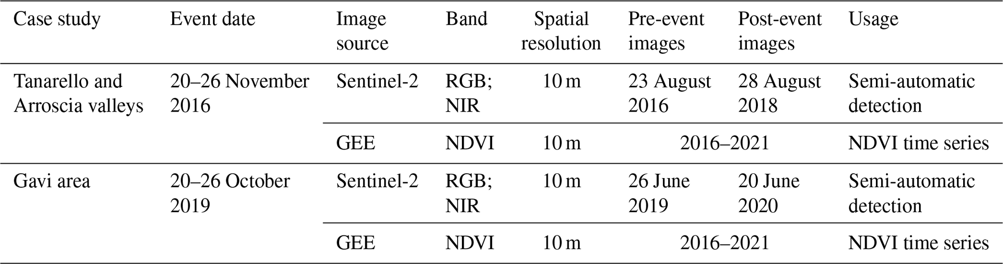
Following the methodology described in Sect. 3.1, we first selected the pre- and post-event images. For our case studies, we used the data of Sentinel-2 satellites (bottom-of-atmosphere reflectance in cartographic geometry – L2A) available on the Sentinel Hub portal (Copernicus Open Access Hub, 2023). In particular, we downloaded the 10 m resolution bands visible (B2, B3, B4) and near-infrared (NIR – B8), and we clipped the original datasets on the area of interest. The datasets used in this study are listed in Table 1. For the Gavi area, we find a pair of images with a 1-year interval, while for the Tanarello and Arroscia Valley areas, the best pair of cloud-free images is on a 2-year interval.

Table 1 Sentinel-2 images used in the selected case studies.

In the second step, we defined the NDVI_var and geomorphological thresholds. In our case study, we used NDVI_var ≤ −0.15 joined to slope > 15^∘ entry values to create the Boolean raster where the value 1 identifies the potential landslides. The slope models were computed from 5 m DTM available from the databases of the Piemonte and Liguria regions and were adopted to the spatial resolution of Sentinel-2 in the raster calculator of QGIS (i.e. it averages the values of four cells of 5 × 5 m into one cell of 10 × 10 m). The Boolean raster keeps the same spatial resolution as Sentinel-2 (10 × 10 m pixel).

We used additional geomorphological thresholds, such as the median slope of the PL polygons. The values were based on the statistical distribution of the ML median slope. We used the filter values' median slopes ≥ 17^∘ and ≥ 20^∘ for the Tanarello and Arroscia Valley areas and the Gavi area, respectively.

In the Tanarello and Arroscia Valley case, we removed the polygons nearby (using an empiric buffer from 5 to 10 m) the hydrographic network to remove false positives related to riverbank erosion. We also filtered the areas in a constant shadow because of a cliff, using threshold values of the averaged means of the four 10 m bands (RGB and NIR) of Sentinel-2 images. The PL polygons were finally smoothed and merged if their distance was lower than 1 m.

3.2.2 High-resolution images for ML inventory

For our study, we employed a stringent calibration and validation methodology in both of our study areas, with an equal ratio of 1 : 1. This differs from the commonly used approach in the literature of a 7 : 3 ratio, as reported in studies such as Mondini et al. (2011) and Mohan et al. (2021). Our decision to utilise this methodology was motivated by the fact that it was our first time implementing this approach. Furthermore, we employed a statistical validation method that is user-friendly and straightforward to replicate in future studies.

For the Tanarello–Arroscia case, the training–validation area is about 300 km², while it is 50 km² for the Gavi 2019 case.

Concerning the Gavi area case study, we applied the proposed methodology as in an ordinary scenario; therefore, we performed over 10 % (about 50 km²) of the area training and validation, and then, with the previously defined parameters, we applied the method to 90 % (500 km²) of the area, producing the inventory. The large 2019 area is also intended to be used as a test inventory for other studies.

Table 2 High-resolution images used for ML mapping in this work.

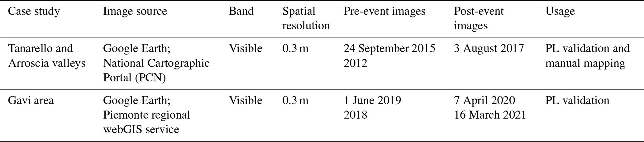
The manual mapping of the landslides was made (in early 2022) on very-high-resolution post-event images. In our case study, high-resolution images were available for both areas, dating back to a few months after the events (Table 2). We used the post-event satellite images available on Google Earth uploaded as an XYZ tile layer on QGIS software (Hafen, 2022). We also used pre-event high-resolution orthoimages available as a web map service (WMS) on the national cartographic service of Italy or the regional web map service of the Piemonte and Liguria regions.

The manual polygons of landslides (MLs) were drawn following geomorphological criteria with the help of shaded relief DTM. Two operators manually checked the inventories to reduce the subjectivity of mapping. The landslide mapping was made on QGIS with the support of Google Earth Pro for historical image visualisation.

3.2.3 NDVI time series analysis using GEE

We also use GEE's potentiality to check and compare the NDVI time series affected by shallow landslides. We manually draw some sample polygons on the GEE interface, imported as feature collections representative of different conditions (landslide/no landslides) and land use. As for the choice of the best images described in Sect. 3.1, we use code based on Nowak et al. (2021). We also extract the NDVI time series using the GEE time series explorer QGIS plugin (GEE Timeseries Explorer, 2020​​​​​​​); such script allows for producing single-pixel time series directly from a point vector. The time series analysis aims to estimate vegetation recovery in the area affected by shallow landslides and to compare it with healthy areas. The vegetation recovery helps assess the maximum period in which a post-event image can be used to calculate NDVI_var. The NDVI time series located in different land uses were also compared using GEE.

3.3 PL and ML inventory comparison and statistics

We compared the PL with ML to evaluate the efficiency of semi-automatic detection by using geoprocessing tools in a GIS environment. Results were synthesised in a validation matrix. The graphical sketch in Fig. 4 shows all the possible combinations. PL and ML vector layers were merged in a unique layer to obtain the intersections between the two datasets, thus getting true positives (TPs), then by selecting residual PL (i.e. parts not included in the intersection) touching or not touching the intersection, partial positives (PPs) and false positive (FPs) were detected. On the other hand, partial detections (PDs) and false negatives (FNs) were defined, respectively, by residual ML touching the intersection sector and ML not intersecting with PL. The five categories were merged in a unique vector layer for further analysis, with the aforementioned classification stored in the attribute table.

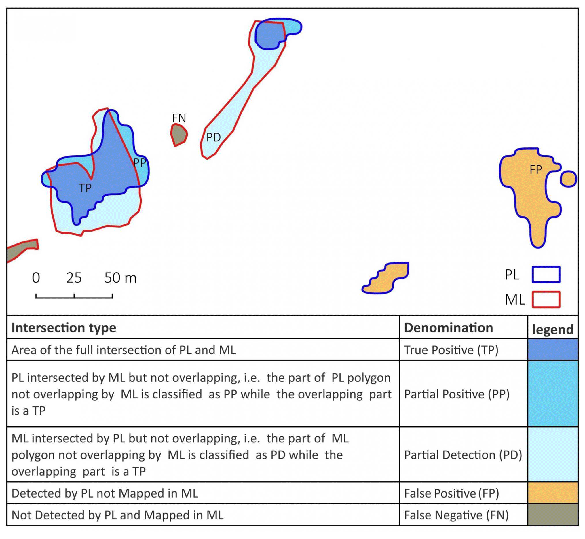
Figure 4 The five possible combinations of PL–ML intersection cases with their description.

The three intersections involving PL (TP, PP and FP) were used to analyse and validate the semi-automatic methodology. Then, by overlaying them on the NDVI and slope angle raster layer, mean values were calculated and stored for each feature. Those values were then processed to obtain descriptive statistics and frequency distributions in terms of the previously described categories. The ML–PL comparison of datasets was also used in an iteration process to enhance the parameters to obtain the PL. The characteristics of FP and TP (e.g. slope and NDVI_var distribution) allowed for improving the filters in semi-automatic detection. We applied some equations similar to those commonly used in the literature (Prakash et al., 2021; Nava et al., 2022; Catani, 2021) to check the quality of automatic mapping. Thus, the false positive rate (FPR; Eq. 2) measures the percentage of the area not correctly detected, and the detection rate (DR; Eq. 3) is the percentage of shallow landslides (both fully and partially) detected by the PL methodology. We also analyse the factors influencing the DR, such as shallow landslide dimension or land use.

$$\begin{array}{}\text{(2)}& {\displaystyle }\mathrm{FPR}=\left(\mathrm{FP}\right)/\left[\right(\mathrm{FP})+(\mathrm{TP})+(\mathrm{PP}\left)\right]\text{(3)}& {\displaystyle }\mathrm{DR}=\left[\right(\mathrm{TP})+(\mathrm{PD}\left)\right]/\left[\right(\mathrm{TP})+(\mathrm{PD})+(\mathrm{FN}\left)\right]\end{array}$$

We also compare the PL and ML inventories using the KD maps made with the procedure described in Sect. 3.1.3. The two densities, sampled on the same regular grid, are compared in a scatterplot, and a correlation coefficient is calculated (Benesty et al., 2009).

4 Results and discussion

The proposed methodology was applied to the two case studies of the Tanarello and Arroscia valleys (2016) and the Gavi area (2019). We obtained for both areas PL and ML inventories with more than 1000 shallow landslides mapped for each AOI. Statistics about the efficiency of PL are also presented in the following paragraphs. Finally, other ancillary datasets were compared to analyse shallow landslide distribution characteristics.

4.1 Tanarello and Arroscia Valley study area

The semi-automatic mapping based on NDVI_var of pre-event (23 August 2016) and post-event (28 August 2018) Sentinel-2 images for the Tanarello and Arroscia Valley study area provided 1056 PLs.

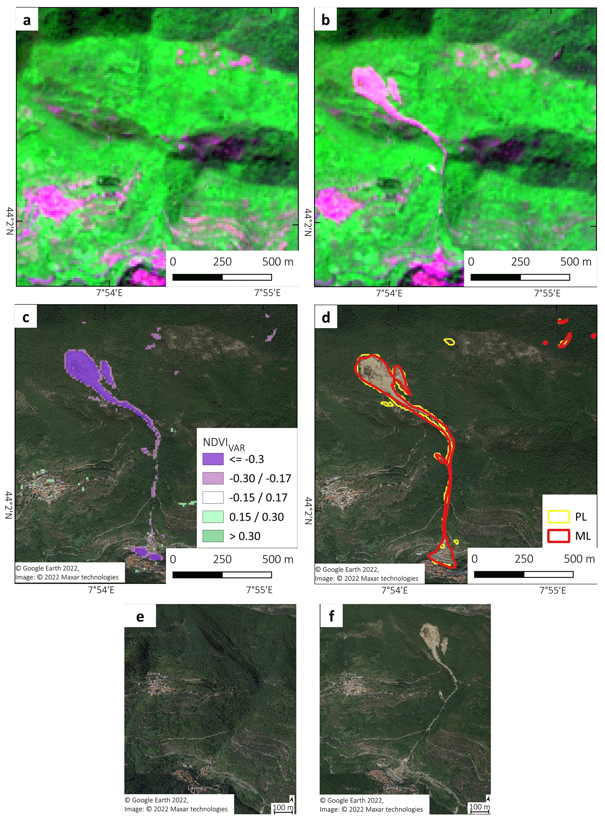
Figure 5 Example of shallow landslide detection methodology for the Tanarello and Arroscia Valley case study: (a) Sentinel-2 pre-event images (RED-NIR-BLUE) acquired on 23 August 2016, (b) Sentinel-2 post-event images (RED-NIR-BLUE) acquired on 28 August 2018, (c) NDVI_var map PL inventory, and (d) ML and PL inventory overlapped with a post-event high-resolution image (Google Earth – 2017). Google Earth 3-D view of (e) pre- and (f) post-events of the area affected by landslides. Map data: © Google Earth 2022; image: © 2022 Maxar Technologies.

Figure 5 shows an example of the steps and results of our methodology over a sample area of the Arroscia–Tanerello case study. From the comparison of pre- (Fig. 5a) and post-event images (Fig. 5b), we obtained the NDVI_var that was used to extrapolate the PL (Fig. 5c). Figure 5d compares the ML drawn on high-resolution Google Earth satellite images and the PL. A detailed 3-D view from Google Earth Pro of pre- and post-event images is shown in Fig. 5e and f.

4.1.1 PL density and distribution

The distribution and kernel density (KD) (search radius 1000 m) of PL centroids are shown in Fig. 6a. At the basin scale, there is a high density of PL in the central sector, particularly in the Arroscia, Armetta and Tanarello valleys, where the density reaches a peak of 10 centroids km⁻². Moreover, Fig. 6b shows a PL detail corresponding to riverbank erosion not filtered out because the hydrographic network has no precise high-resolution geocoding, and the derived 5 m buffer did not intersect the PL. It is challenging to create an affordable geomorphological filter discriminating river erosion from a shallow landslide in a steep valley, and in many cases, the two processing overlap or are linked by a cause–effect relationship. Figure 6c shows the correct detection of a landslide; its shape is almost accurate considering the Sentinel-2 resolution, while Fig. 6d shows a shallow landslide not detected (false negative case) because the shadow mask filters it out.

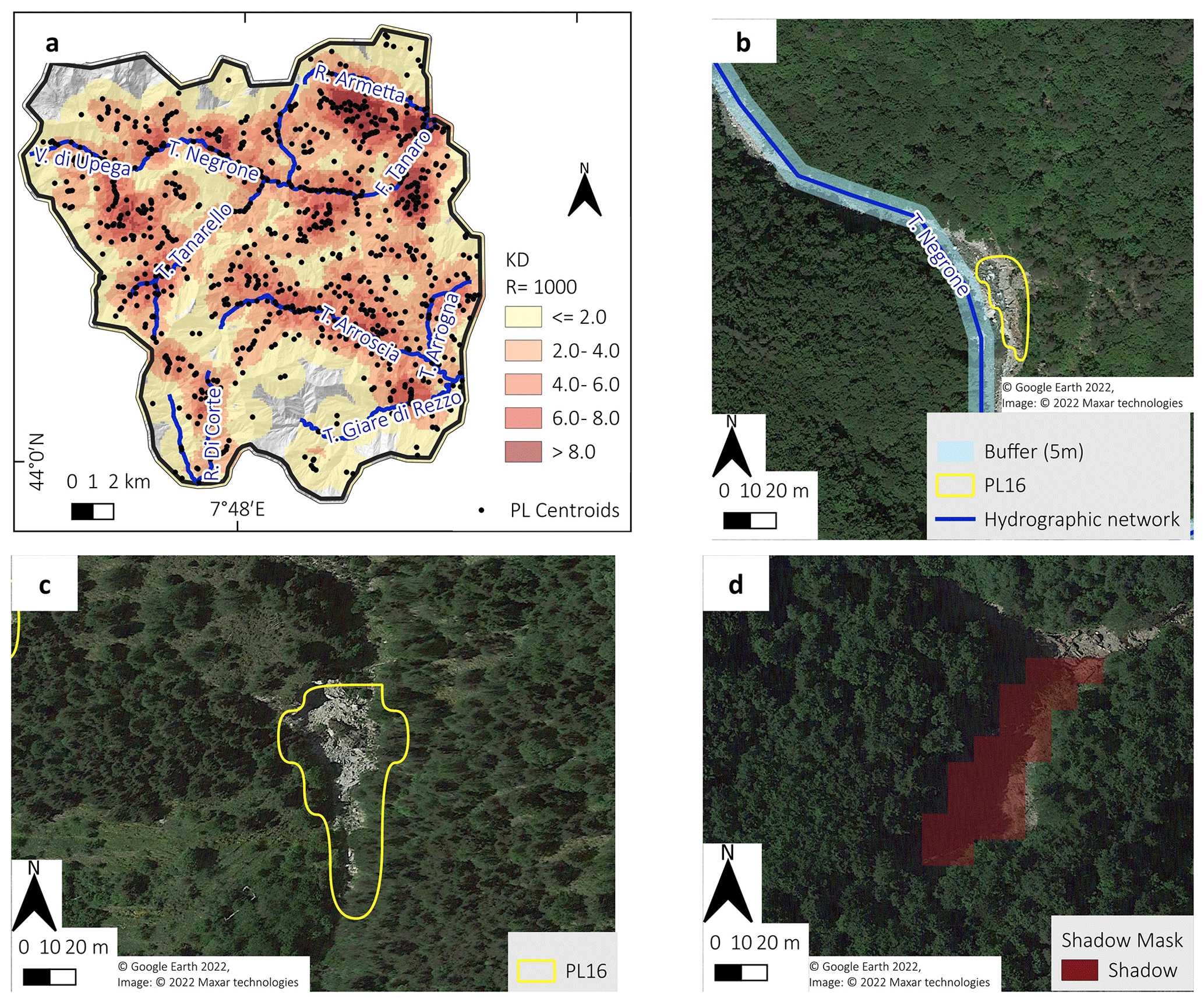
Figure 6 (a) The kernel landslide centroid relative density (search radius = 2500). (b) Detail of PL representing a riverbank erosion, (c) PL that correctly detects the shallow landslide, (d) shallow landslides not detected by PL because it is filtered with a shadow mask. Map data: © Google Earth 2022; image: © 2022 Maxar Technologies. The shaded relief of map (a) is based on 5 m DTMs of ARPA Piemonte and Liguria.

4.1.2 PL and ML intersection results

The manual mapping of landslides made on post-event Google Earth and high-resolution satellite images was compared with pre-event aerial photos of 2012 (MASE, 2012) and allowed for the detection of 1098 MLs (average density 3 ML km⁻²). The intersection of PL and ML datasets produced about 2620 cases.

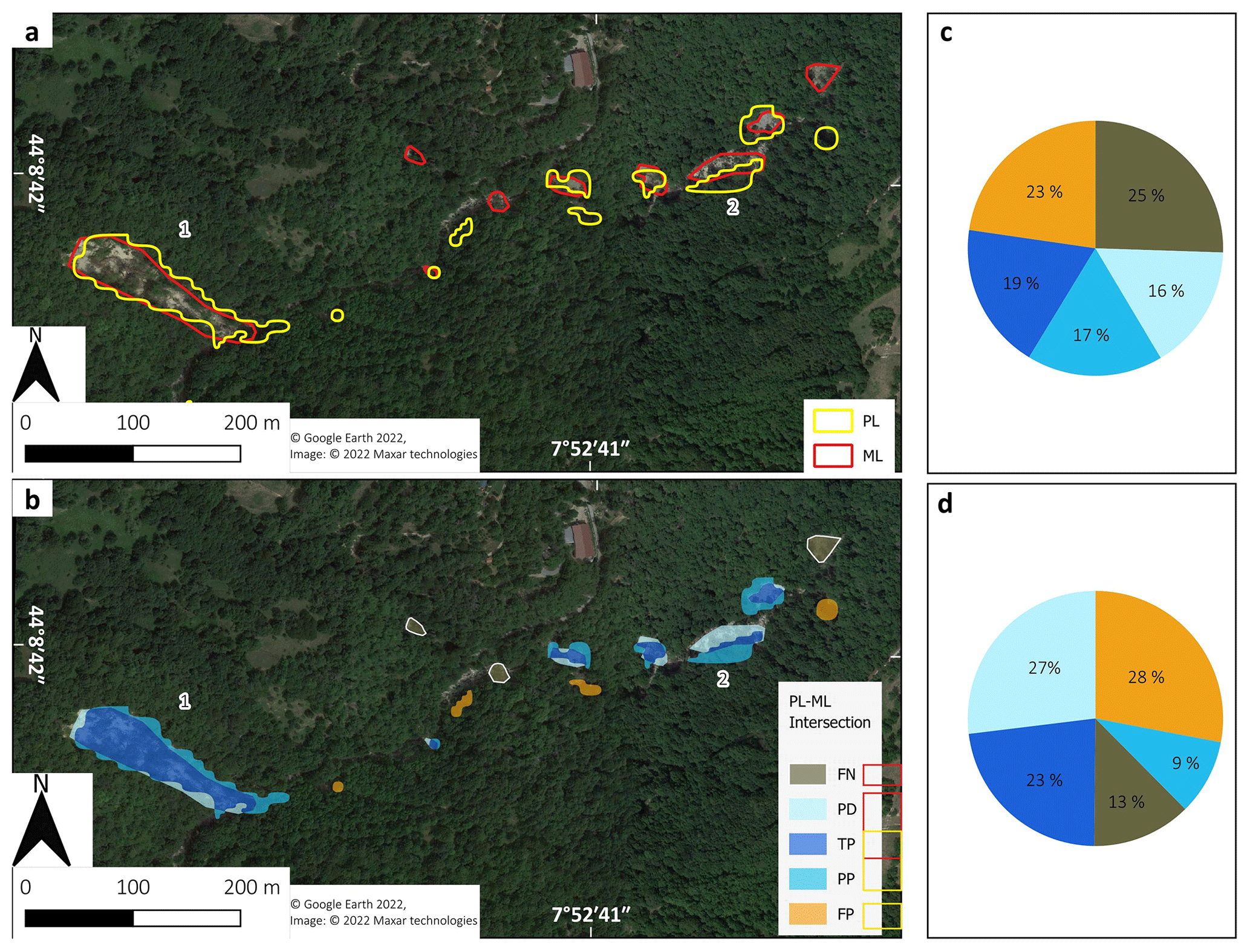
Figure 7 The Tanarello and Arroscia Valley case study. (a) The PL–ML inventory intersections over a sample area. (b) The PL–ML intersection classified by type. Pie charts of the intersection type distribution by (c) number and (d) area. Map data: © Google Earth 2022; image: © 2022 Maxar Technologies.

Figure 7a shows, over a sample area, some examples of the intersection between PL and ML inventories. In Fig. 7b, the intersections are classified into the five types of combinations defined in Fig. 4​​​​​​​. In some cases, the PL–ML overlapping (TP) is almost complete (intersection 1) in Fig. 7a and b, while in others (intersection 2), TP cases represent a small portion of the intersection. For the whole Tanarello and Arroscia Valley case study, we also reported the intersection case pie charts by polygon count (Fig. 7c) and total area (Fig. 7d). It can be noted that the biggest difference between count and area statistics (25 % to 13 %) is for the FN case because it corresponds to many MLs with a small area. In contrast, FP shows a slight increase because the size of PLs is always more than 100 m² (i.e. the Sentinel-2 spatial resolution).

4.1.3 PL validation statistics

Detailed validation results for PL made with R (see Sect. 3.3) are shown in Fig. 8. The chart of Fig. 8a shows the number distribution of TP, PP and FP cases. The TP represents about 32 % of intersected PL summed with the PP, representing 29 % of intersections, showing that the methodology correctly detects a shallow landslide in 60 % of cases. The area frequency distribution chart (Fig. 8b) indicates that the PP cases have smaller areas (median 165 m²) than the TP (230 m²) cases; this means that the TP increases in up to 38 % of the cases considering the area sum instead of the polygon count. Several FP cases correspond to fluvial processing like bank erosion that filters could not remove. Some other regions correspond to artificial forest cuts that occurred from 2016 to 2018. In addition, the only complete summer cloud-free pair of images is August 2016 vs. August 2018, and this extended period increased the probability of detecting land-use change not related to landslides.

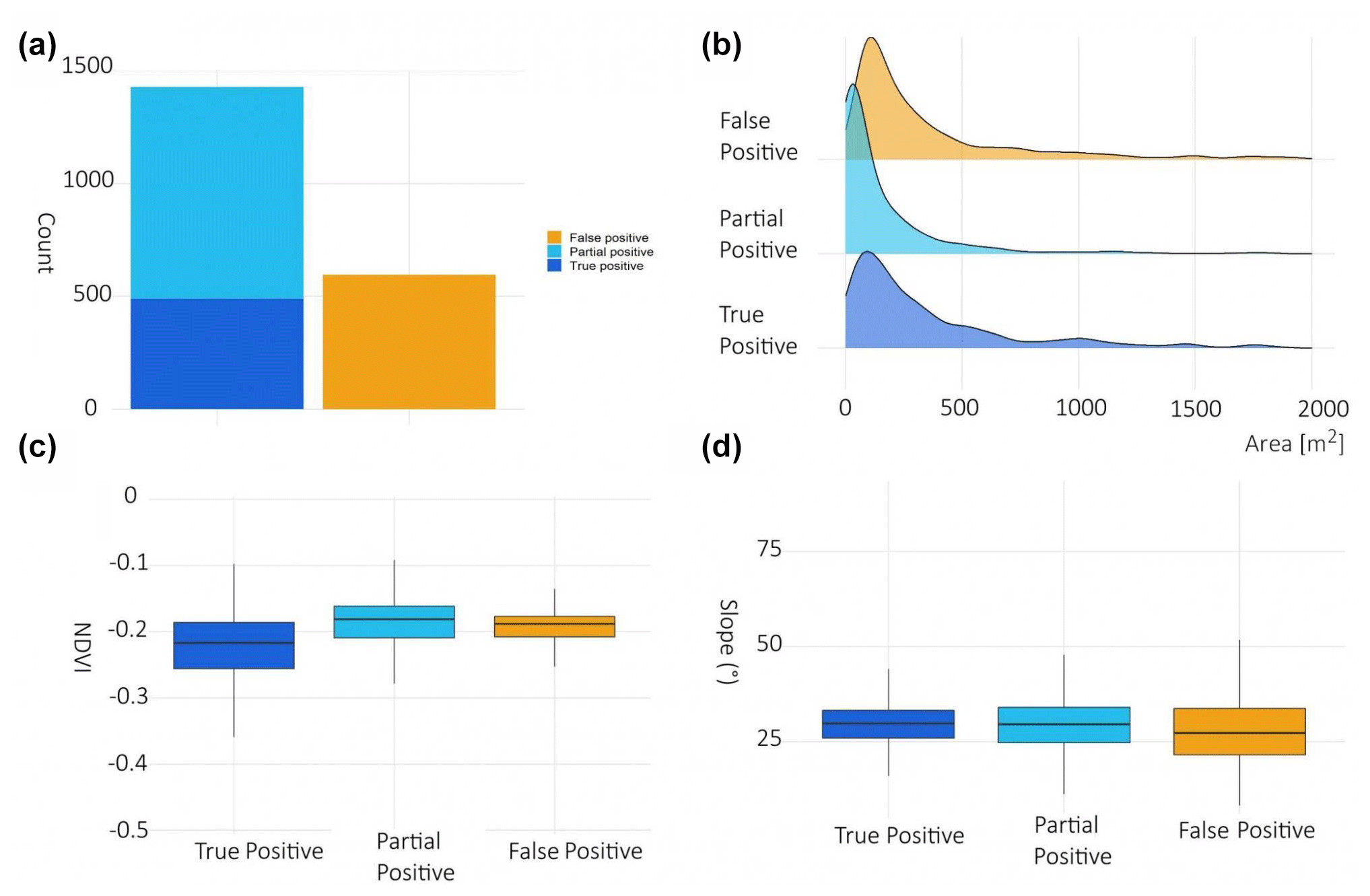
Figure 8 PL validation statistics for the Tanarello and Arroscia Valley case study: (a) bar plot showing the number of polygons of PLs classified as TP, PP, and FP areas; (b) area frequency distribution of the polygons classified as TP, PP, and FP areas; (c) boxplot chart of NDVI_var distribution for TP, PP, and FP classes; and (d) boxplot chart of median slope distribution for each class of the ML–PL intersection.

The NDVI_var and the slope are the main parameters used to detect landslides; therefore, their distribution inside the intersected PL–ML inventories helped us to understand the efficiency of the semi-automatic approach. Figure 8c shows the median NDVI_var for each class of ML–PL intersections. The TP cases show NDVI_var values below the −0.16 threshold, probably because the shallow landslides strongly impact vegetation compared to other land-use changes. Figure 8d shows the median slope distribution; in this case, there are few differences among the classes because the slope filter (17^∘) removed most FPs related to the slope gradient. This means that most FP cases are caused by a land-use change or riverbank erosion with the same slope gradient of shallow landslides.

The FN and PD intersection cases are discussed in Sect. 4.3.1 because they are not coming from PL and are not related to parameters used for PL methodology but to the relation of landslide size with the spatial resolution of the satellite.

4.2 Gavi area case study

For the Gavi area case study, we used the Sentinel-2 20 June 2019 (pre-event) and 26 June 2020 (post-event) images. The semi-automatic mapping allowed us to obtain about 1077 PLs inside the training area and about 3100 in the whole study area.

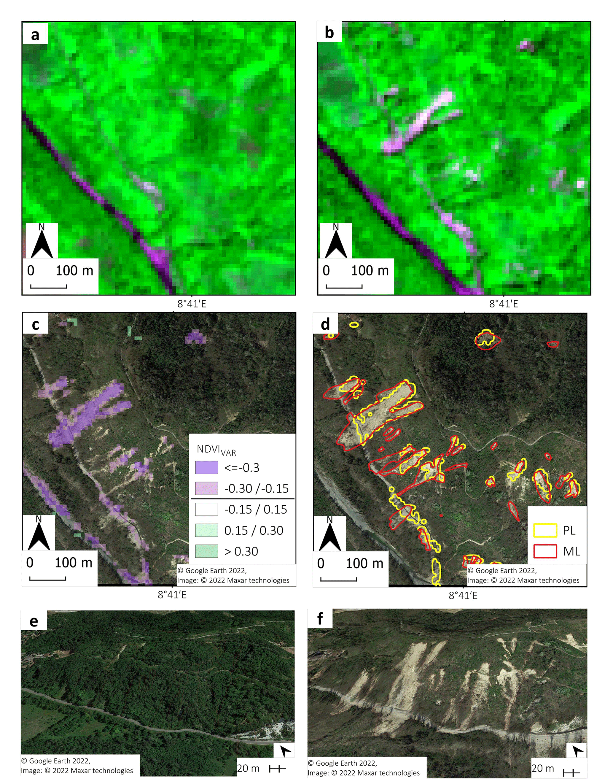
Figure 9 Example of shallow landslide detection methodology for the Gavi 2019 case: (a) Sentinel-2 pre-event images (RED-NIR-BLUE) acquired on 20 June 2019, (b) Sentinel-2 pre-event images (RED-NIR-BLUE) acquired on 26 June 2020, (c) NDVI_var map overlapped with a Google Earth post-event image, and (d) comparison of ML and PL inventories overlapped with a Google Earth post-event image. Google Earth 3-D view of (e) pre- and (f) post-events of the area affected by landslides. Map data: © Google Earth 2022; image: © 2022 Maxar Technologies.

Figure 9 shows an example of the steps and results of our methodology over a sample area of the Gavi 2019 case study. From the comparison of pre- (Fig. 9a) and post-event images (Fig. 9b), we obtained the NDVI_var (Fig. 9c), which was used to extrapolate the PL. Figure 9d​​​​​​​ compares the ML drawn on high-resolution Google Earth satellite images and the PL. A detailed 3-D view from Google Earth Pro of the pre- and post-event is shown in Fig. 9e and f.

4.2.1 PL density and distribution

Figure 10 shows the kernel centroid density (based on a search radius of 1000 m) and distributions for the PL inventory (Fig. 10a). About 3000 PLs were identified using the parameters and the filters described in the methodology section; 1100 of them are inside the training area. It can be observed that the training and validation areas show the highest PL density. Other areas of high PL density are located north of Ovada and south of Acqui Terme. Here, manual mapping on high-resolution (HR) images is proposed for further manual mapping. It is possible to analyse the different cases of PL methodology results in more detail. Figure 10b shows the correct detection of a landslide, and its shape is almost accurate considering the Sentinel-2 resolution. Figure 10c shows a PL that partly detected shallow landslides: in many cases, the trigger points are detected because of their abrupt changes, while the bottom part with more shallow sediment flow is not detected. Two small shallow landslides not caught on Sentinel-2 images are also shown. Figure 10d shows a false positive case where PL most probably detected a change in vegetation activity within a vineyard.

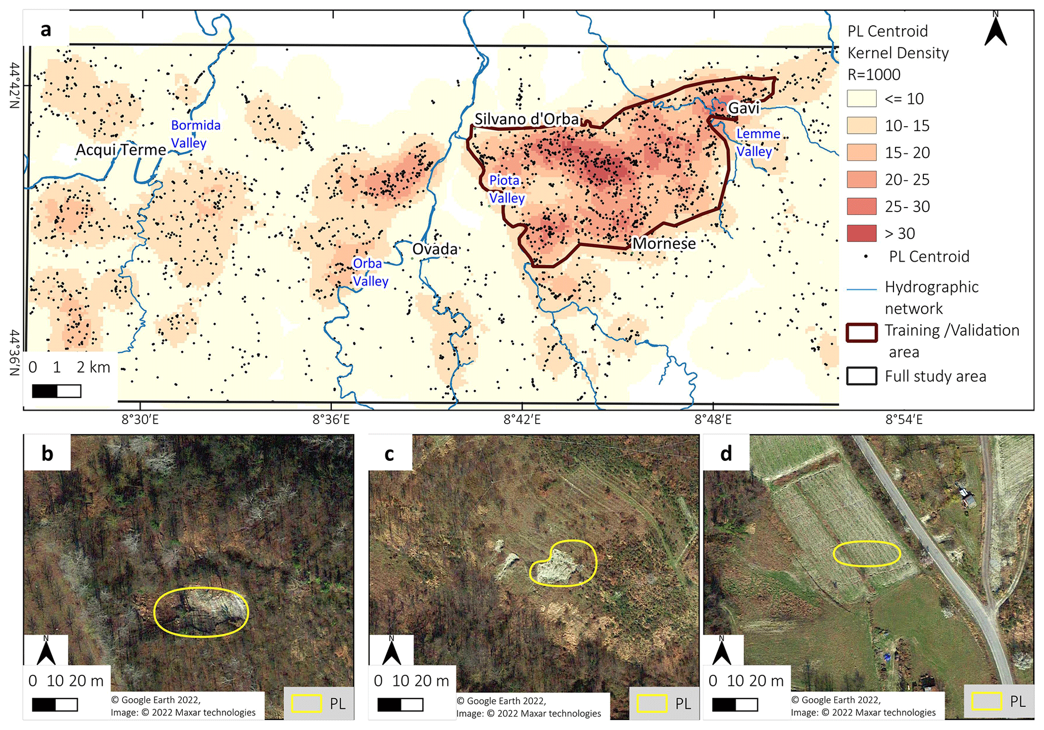
Figure 10 The October 2019 event. (a) PL centroid relative kernel density (R = 1000) over the whole AOI. Some examples of PL: (b) PL that completely overlaps a shallow landslide, (c) PL that partly overlaps a shallow landslide, and (d) PL that corresponds to a false positive case. Map data: © Google Earth 2022; image: © 2022 Maxar Technologies. The shaded relief of map (a) is based on the 5 m DTM of ARPA Piemonte.

4.2.2 PL and ML intersection results

Also, for the Gavi area case study, we made similar statistics for the inventory intersection used for the Tanarello and Arroscia Valley case study. The manual mapping of landslides, made on post-event Google Earth, and high-resolution satellite images compared with pre-event aerial photos of 2018 (Regione Piemonte, 2020) resulted in 1178 MLs (average density 23 ML km⁻²). The intersection of PL and ML datasets produced about 2982 cases.

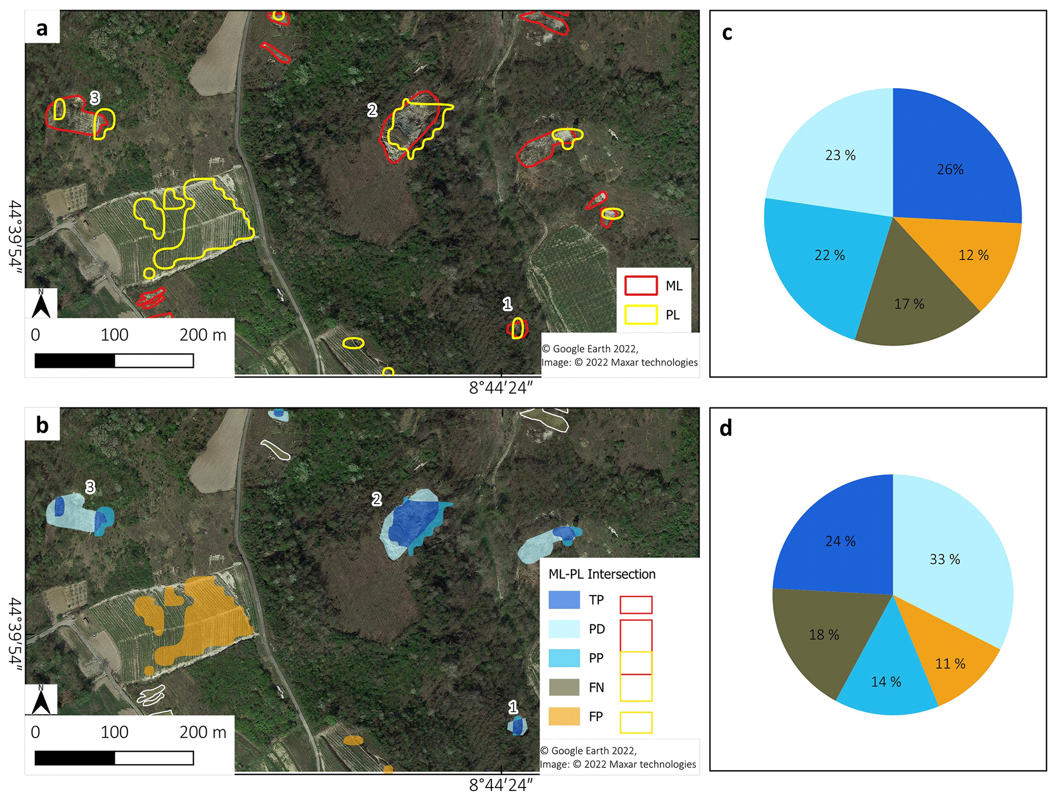
Figure 11 The 2019 Gavi case study. (a) The PL–ML inventory intersections over a sample area. (b) The PL–ML intersection classified by type. Pie charts of the intersection type distribution by (c) number and (d) area. Map data: © Google Earth 2022; image: © 2022 Maxar Technologies.

Figure 11a shows, over a sample area, some examples of the intersection of PL and ML inventories. In Fig. 11b, the intersections are classified into the five types of combinations (TP, FP, FN, PD and PP) defined in Fig. 4. In some cases, the PL–ML overlapping (TP) is almost complete (case 1) or partial (case 2). In other cases (3) the PL allowed us to detect only a tiny portion of the intersection, and most of the shallow landslide area was classified as PD. For the whole 2019 study area, we also represented the intersection case pie charts by polygon count (Fig. 11c) and area (Fig. 7d). It can be noted that in contrast to the 2016 case, there is little difference between the count by number or total areas. The different distributions of ML size (see Fig. 13b) could explain this.

4.2.3 PL validation statistics

Detailed validation statistics results for PL made with R (see Sect. 3.3) are shown in Fig. 12. The chart of Fig. 12a shows the number distribution of TP, PP and FP cases. The TP represents about 43 % of intersected PL summed with the PP, representing 37 % of cases, showing that the methodology correctly detects a shallow landslide in 80 % of cases. The results of semi-automatic mapping for the Gavi AOI are better than for the Arroscia–Tanarello AOI. The better performances could be explained by a better pair of pre- and post-event images and the stronger magnitude of the 2019 event. The area frequency distribution chart (Fig. 12b) shows that the partial positive cases have smaller areas (median 165 m²) than TP (230 m²); this implies that the percentage of TP rises from 43 % to 49 % of PLs considering the area sum instead of polygon count. FP cases generally correspond to changes in agriculture activity that occurred in 2019–2020 in the vineyard. As previously stated, NDVI_var and slope were analysed in terms of intersection class and provided the same insight concerning the influence of vegetation health and acclivity.

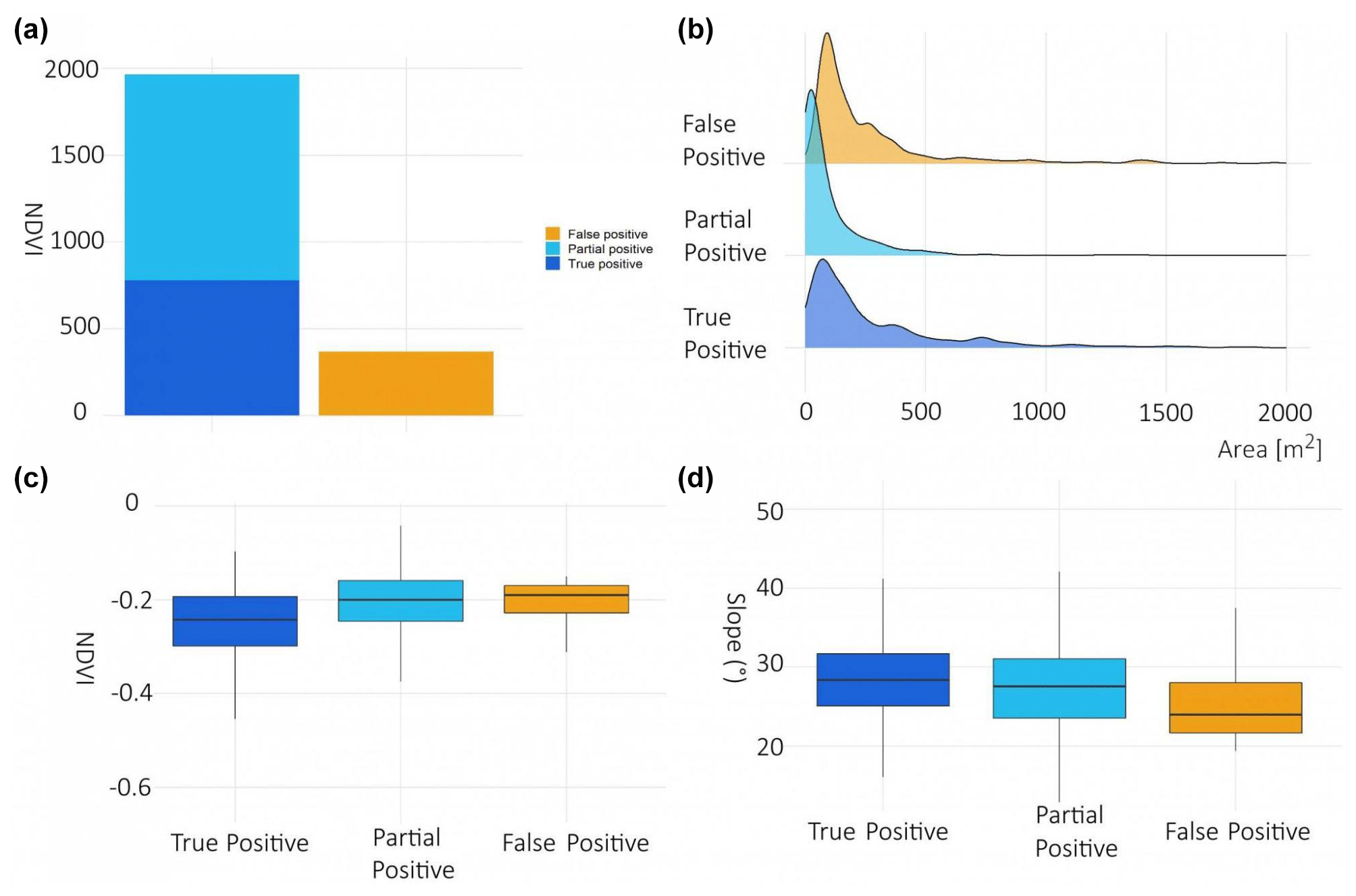
Figure 12 PL validation statistics for the 2019 Gavi study area: (a) bar plot showing the number of polygons of PL classified as TP, PP, and FP areas; (b) area frequency distribution for the polygons classified as TP, PP, and FP areas; (c) boxplot chart of NDVI_var distribution for TP, PP, and FP classes; (d) boxplot chart of median slope distribution for each class of the ML–PL intersection.

As mentioned in the Tanarello and Arroscia case study (Sect. 4.1.3), The FN and PD intersection cases are discussed in Sect. 4.3.1.

4.3 Factors that influence shallow landslide detection and false positives

In this section, we discuss the main factors that, according to our results, influence the efficiency of the proposed PL methodology. As already done in the literature, the landslide size (Bellugi et al., 2021; Fiorucci et al., 2018), land use (Mondini et al., 2011) and temporal interval (Lindsay et al., 2022; Scheip and Wegmann, 2021) used in the pre- and post-event calculation seem the most interesting to discuss on the basis of our results.

4.3.1 Shallow landslide size, density and distributions

The detection capacity is mainly related to shallow landslide size and the spatial resolution of Sentinel-2.

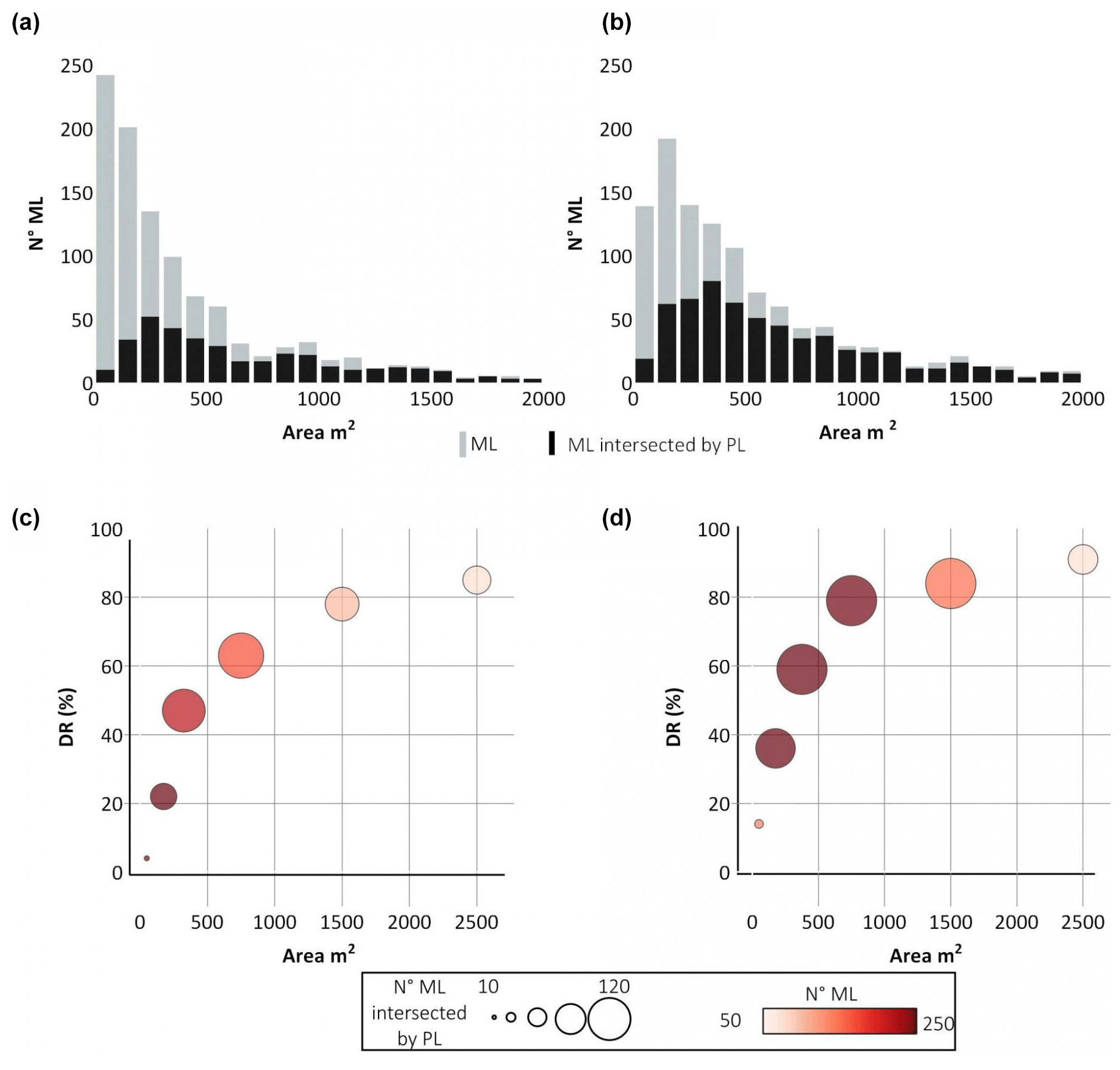
Figure 13 Histogram of ML area distribution for the Tanarello and Arroscia valleys (a) and Gavi (b) study areas: the grey bars represent the entire ML inventory, while the black ones represent the ML intersected by a PL. The detection rate (DR) for each area class for the Tanarello and Arroscia Valley (c) and Gavi area (d) case study. The size of the circle is correlated with the number of detected MLs; the colour scale represents the total number of MLs for each class.

Figure 13a and b show the histogram distribution of ML size for the Tanarello and Arroscia valleys and Gavi study areas, respectively. The ML size distribution agrees with the classical power-law distribution of shallow landslides (Bellugi et al., 2021; Guzzetti et al., 2002) for both cases studied. This means that the shallow landslides smaller than 500 m² are about 60 % of all ML inventories, but they represent only 20 % of the total area affected. The histograms also show that for the Tanarello and Arroscia valleys (Fig. 13a), the MLs are generally smaller than in the Gavi area. The parts of the bars that are black coloured show the ML intersected by PL (TP + PD intersection cases). It is possible to note that the small landslides (100 m²) are underestimated by PL, while for large landslides, PL almost fits the ML. These results agree with the area frequency distribution for TP and PD cases shown in Figs. 8b and 12b.

Figure 13c and d show the DR calculated with Eq. (2) for the Tanarello and Arroscia valleys and Gavi study areas. The DR increases with the size of the landslides, and it is strictly related to the pixel size of Sentinel-2. For the landslides smaller than 100 m² (Sentinel-2 spatial resolution), the DR ranges from 10 % for Tanarello and Arroscia Valley (Fig. 13c) to 15 % for the Gavi area (Fig. 13d). It is clear that for these landslides, the Sentinel-2 platform is not the optimal choice (Fiorucci et al., 2018), and manual mapping on high-resolution images is better than semi-automatic mapping. On the other hand, for the ML in the class area (500–1000, i.e. 5–10 pixels of a Sentinel-2 image), the DR ranges from 65 % for Tanarello and Arroscia Valley to 80 % for the Gavi area.

The overall DR considering polygon count is 39 % for the Tanarello and Arroscia Valley and 58 % for the Gavi case study, while considering the area sum, the DR is 60 % and 75 %, respectively. The Gavi case study's better performance is likely related to the size distribution of shallow landslides and the better pair of images used to create PL.

The performance metrics precision (P) P = TP $/$ (TP + FP), recall R = TP $/$ (TP + FN) and F₁ score F₁​​​​​​​ = 2TP $/$ (2TP + FP + FN) without considering the intersection cases are reported in Table 3. The overall performance of our methodology is comparable with other studies, especially those using middle-resolution images (Ghorbanzadeh et al., 2021; Mondini et al., 2011; Handwerger et al., 2022). A recent study (Ganerød et al., 2023) using Sentinel-2 has shown different performances depending on the study area in Norway; the best is from the deep-learning approach with a U-net architecture. Using high-resolution Planet images (Bhuyan et al., 2023) achieves high performance over several study areas. However, we assume that the different study/training/validation settings, the image used and the event type made this comparison relative.

Table 3 Performance metrics of this methodology.

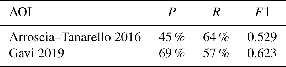
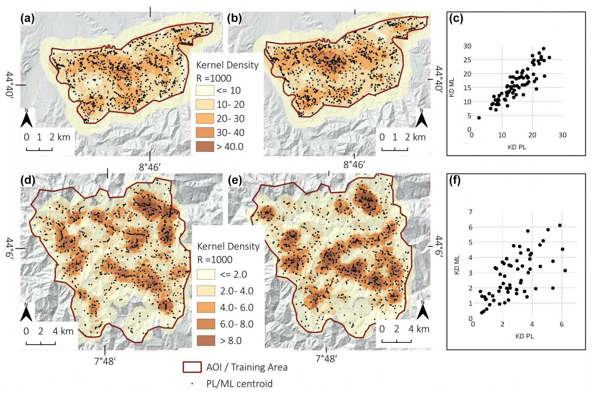
Figure 14 Heatmap kernel density for the (a) Gavi PL inventory, (b) Gavi ML inventory, (d) Tanarello and Arroscia Valley PL inventory, and (e) Tanarello and Arroscia Valley ML inventory. Scatterplot of ML–PL kernel density comparison for the (c) Gavi training area and (f) Tanarello and Arroscia Valley study area. Shaded reliefs of maps (a), (b), (d) and (e) are based on 5 m DTMs of ARPA Piemonte and Liguria.

Both in the Tanarello and Arroscia valleys and Gavi areas do the results of spatial correlation of ML and PL density show a good agreement (Fig. 14), a further confirmation of the effectiveness of the PL methodology. Specifically, in the case of 2019, both ML and PL inventories, Fig. 14a and b, show a higher density in the northern sector of the study area and a lower density in the central region. Figure 14c shows the scatterplot between the PL and ML density; the correlation coefficient (Benesty et al., 2009) has a value of 0.85 with an R² = 0.73 using a grid of 1000 m. Moreover, the average ML density is about 23 ML km⁻² higher than the 2016 event (3.1 ML km⁻²). The difference is probably related to the more intense rainfall of October 2019 (up to 500 mm in 24 h) compared to the 2016 case (700 mm in 5 d).

We also manually checked Google Earth and noticed the same performance in a small validation area outside the Gavi training area.

In the case of 2016, there are more discrepancies. A higher density of PL in the NE sector (Fig. 14d) can be noted. At the same time, ML shows a density peak in the Arroscia Valley (Fig. 14e). Both datasets show that centroids' high density is located in the central sector, particularly in the Arroscia, Armetta and Tanarello valleys, where the density reaches a peak of 10 centroids km⁻². At the basin scale, PL–ML regressions show a correlation coefficient of 0.68 with an R² = 0.47 using a grid of 2500 m (Fig. 14f).

4.3.2 The effect of land use on PL methodology efficiency

We deeply investigate the role of land use in landslide detection. The semi-automatic detection performed well for naturally vegetated slopes, while the detection capability decreased for cultivated landscapes.

For instance, the statistics on intersection cases for the four main land-use classes (Land Cover Piemonte, 2022) made for the 2019 case study allowed us to understand the variable regarding the land-use efficiency of semi-automatic mapping.

The forest and the new forested shrub areas (Fig. 15a and b) show a high percentage of TP cases, and about 80 % of PL corresponds to shallow landslides. Here, human disturbances are limited, and the majority of NDVI_var is related to landslides. The FN (15 % of the area) fits small landslides not detectable with Sentinel-2 because of its spatial resolution.

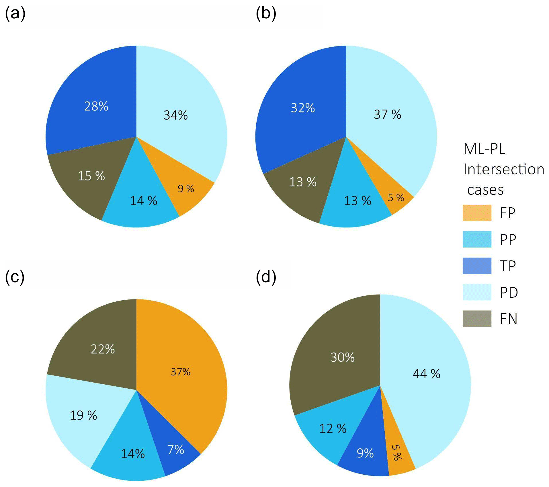
Figure 15 The Gavi 2019 case study. PL–ML intersection distribution for the main land-use classes: (a) broadleaf forest, (b) new forest or shrubland, (c) vineyard, (d) and cultivated land.

The vineyard land use (Fig. 15c) shows a high FP percentage (37 %). In this land use, most FP cases are changes related to vineyard management. FN is also higher (22 %) compared to the forested areas. The cultivated land (Fig. 15d) shows a high percentage of FN (30 %). The underestimation can be explained by smaller landslide dimensions and the agricultural practice that erases the signs of landslides.

4.3.3 NDVI time series based on GEE

Figure 16a and b show the NDVI time series based on Sentinel-2 computed on GEE (see “Data availability” section). The NDVI time series of the area affected by shallow landslides (red line in Fig. 16) is based on averaged NDVI of a subset of ML polygons with an area of at least 500 m². This time series is compared with the time series averaged over a region not affected by landslides (black line in Fig. 16).

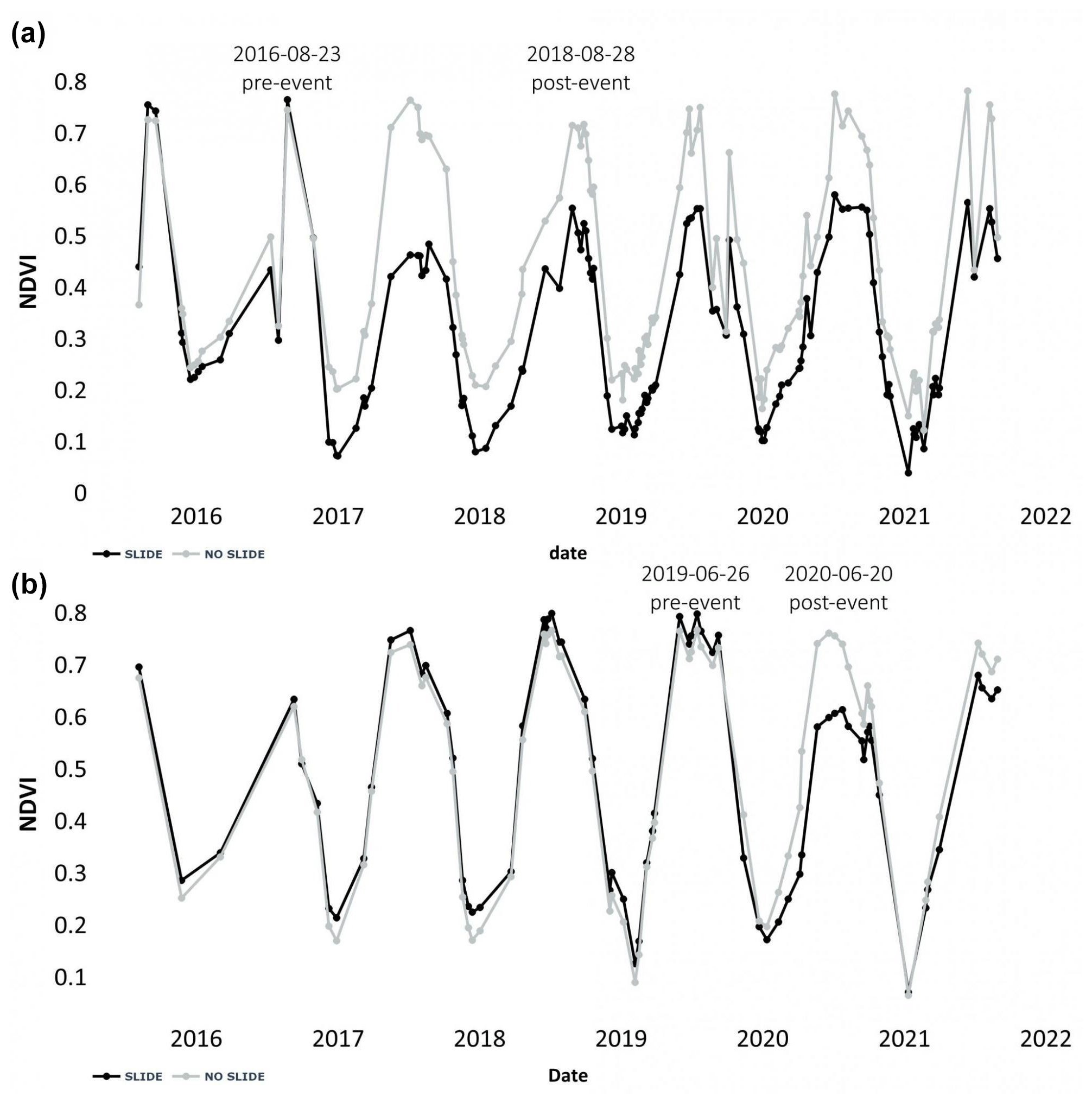
Figure 16 NDVI time series based on Sentinel-2 data and processed with GEE: the “Slides” black lines are the averaged time series of the selected ML; the “no slides” grey lines are the time series of the surrounding unaffected areas. (a) 2016 Arroscia–Tanarello case study; (b) 2019 Gavi case study.

In the case of the Arroscia–Tanarello 2016 study area (Fig. 16a), it can be observed that in the areas not affected by landslides, the NDVI has a relatively constant seasonal trend during 2015–2021, ranging from 0.25 in winter to 0.75 in summer. On the contrary, the areas affected by shallow landslides showed a substantial decrease in NDVI (from 0.75 to 0.4) in the post-event 2017 summer. The NDVI slowly increased during the following years, up to the value of 0.55 in 2021. If we compare the pair images (23 August 2016, 28 August 2018​​​​​​​) used to extract the PL, we can observe an average NDVI_var of −0.2. Unfortunately, the summer 2017 images that show the best NDVI_var are not fully cloud free or are not acquired in the same seasonal period.

In the case of the Gavi case study (Fig. 16b), in those areas not affected by landslides, the NDVI has a constant seasonal trend during the period 2016–2021, ranging from 0.2 in winter to 0.8 in summer. In contrast, the NDVI of the areas affected by shallow landslides shows a substantial decrease, showing a value of 0.6 (−0.2 variation) in the 2020 summer. The NDVI value rebounded to 0.65 in 2021. The pair images (26 June 2019, 20 June 2020) used to extract the PL show an average NDVI_var of −0.15. The vegetation seems to recover faster compared to the 2016 case.

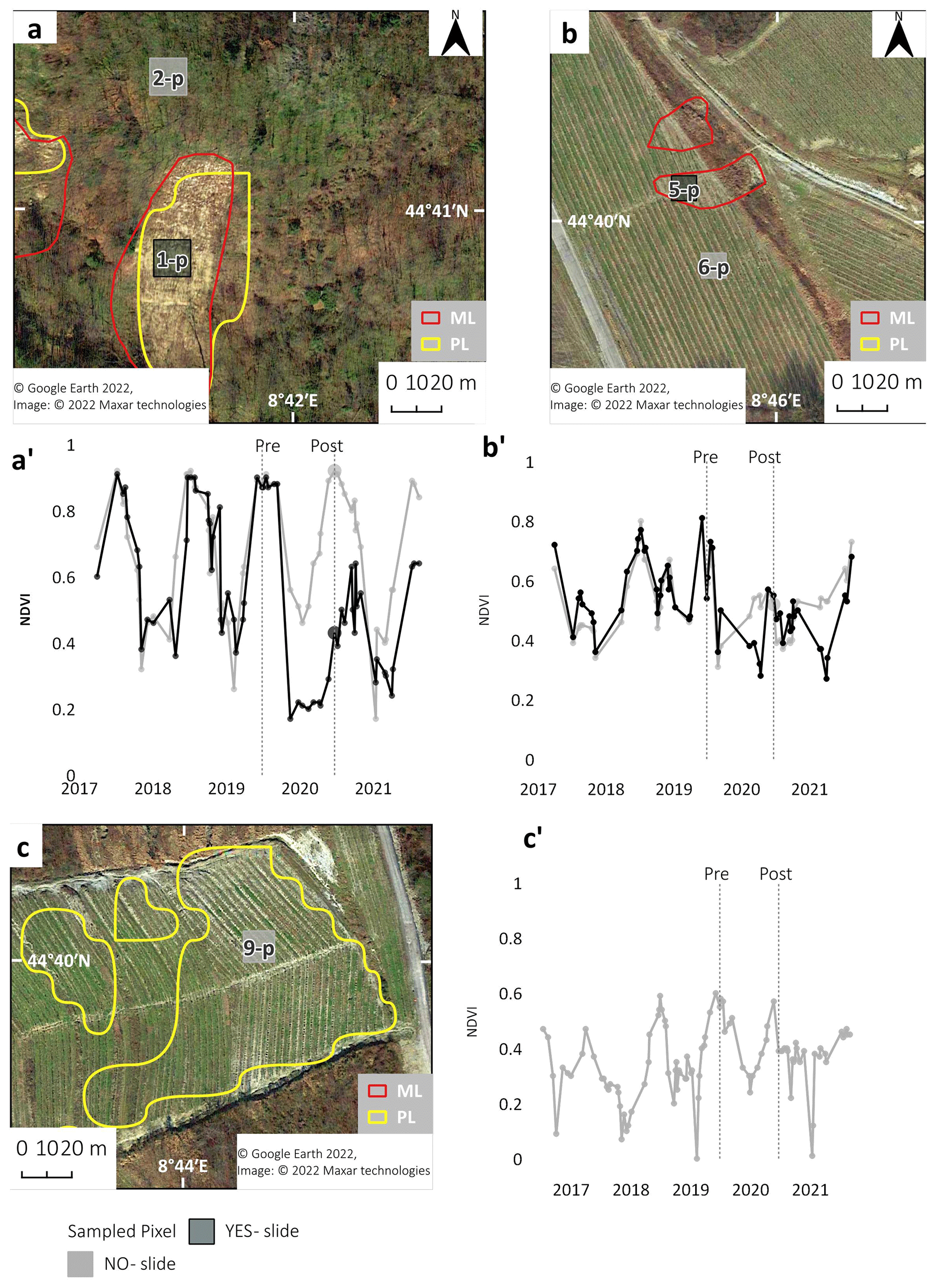
Figure 17 NDVI time series (2017–2021 of five sample points (landslide and no landslide) in the area affected by the 2019 event. (a, a') Comparison located in a broadleaf forest (true positive); (b, b') vineyard (false negative); (c, c') vineyard (false positive). The Google Earth satellite image was acquired on 16 March 2021. Map data: © Google Earth 2022; image: © 2022 Maxar Technologies.

The effects of land use on detection capabilities are difficult to solve with simple filters. A partial solution could be the NDVI time series analysis. The analysis of the single-pixel time series of NDVI, generated with the GEE QGIS plugin (GEE Timeseries Explorer, 2020​​​​​​​), allowed us to better understand the effect of landslide size and land use on the capacity detection of Sentinel-2; the main results are resumed in Fig. 17.

Figure 17a and a' show the location and the comparison of two NDVI time series in a broadleaf forest land use: the 1-p is entirely inside an ML of approximately 1500 m², while the 2-p is an undisturbed area. The two time series show almost the same seasonal trend until the 2019 event; after this, the NDVI of 1-p shows values of 0.2 less than the NDVI of 2-p in the 2020 summer.

Figure 17b and b' show the location and the comparison for two single-pixel time series located in a vineyard land use. In this case, the 5-p is situated in an ML with an approximate size of 500 m² not detected by PL methodology (a false negative case). Both slide (5-p) and no-slide (6-p) NDVI time series show an irregular trend, probably related to the agricultural activity inside the vineyard. The post-event time series shows lower NDVI values for the pixel inside the ML; however, the noise is too high to extract a clear trend.

Figure 17c and c' show the location and NDVI time series of a false positive PL in a vineyard land use (9-p). In this case, the agricultural activity inside the vineyard caused a NDVI_var < −0.16 using the pre- and post-event pair images. However, if we look at the whole time series, there is no trace of the effect of shallow landslides.

Instead of considering single pre- (26 June 2019) and post-event (20 June 2020) dates, the noise could be reduced if we use the averaged pre- and post-event summer (May–September) images. Multi-temporal-averaged satellite data on GEE have already been used to improve landslide detection (Lindsay et al., 2022). For instance, using this approach, the FP of Fig. 17c disappears because the NDVI_var is −0.16 for single pairs, while it is −0.03 for the averaged summer periods.

The summer-averaged pre- and post-event NDVIs computed with GEE for the Gavi area are available in the “Data availability” section.

5 Conclusions

A low-cost semi-automatic methodology to detect shallow landslides using cost-free data from Sentinel-2 satellites was implemented and tested in exemplary cases. The implemented user-friendly processing is aimed to be used by a wide range of final users, such as technicians or natural hazard planners with low expertise in remote sensing processing and computer science. Landslide data and GEE scripts were also available in the free storage database for researcher and community users. We test the methodology on two extreme rainfall events that affected NW Italy in November 2016 (Tanerello and Arroscia valleys) and October 2019 (Gavi area).

We obtain a polygon dataset representing potential shallow landslides (PLs) and their density maps with semi-automatic mapping. The PL density maps aim to identify the most affected areas in which to focus the manual mapping on high-resolution images. The PL dataset is created with a three-step approach: (i) choosing the best pair of Sentinel-2 images also with the help of the NDVI time series computed with Google Earth Engine (GEE), (ii) creating the NDVI_var map from pre- and post-event images, (iii) using geomorphological filters based on slope and other parameters such as distance from the hydrographic network, and (iv) eventually re-calibrating the PL parameters with landslides manually detected (ML). In the study areas of Tanarello and Arroscia Valley and Gavi, 1077 and 2576 PLs were detected, respectively. The areas with the highest PL density also match with areas most affected by rainfall events.

The PL inventory was compared with manual mapping based on high-resolution images in training and validation areas. We manually map landslides on cost-free high-resolution images (e.g. Google Earth, national or regional cartographic services). The manual mapping detected about 1100 MLs over 300 km${}^{{}^{\mathrm{2}}}$ in the Tanarello and Arroscia valleys and about 1180 MLs over 55 km${}^{{}^{\mathrm{2}}}$ in the Gavi area. The PL datasets were then compared (ML). The ML and PL inventory comparison shows a good agreement in density and distributions, especially for the Gavi case study.

According to the findings, the semi-automatic method can detect the majority (about 60 %) of shallow landslides larger than 2 or 3 times the size of Sentinel-2 ground pixels (100 m²). In contrast, the PL method can identify only 20 % of small landslides (less than 100 m² in size). In agreement with the power-law, small landslides are a high number but a small fraction of the affected area. Consequently, the false negative represents 60 % to 40 % of the cases but only 20 %–25 % of the affected area. In the future, using high-resolution cost-free satellite images for semi-automatic methods could drastically increase the detection capacity. Land use is another factor that influences detection capacity: in the Gavi study area, the detection rate reached 73 % on natural vegetation like forest land use, while in cultivated areas, DR decreased by up to 41 %.

The false positive rate (FPR) (28 % for the Gavi area and 48 % for the Tanarello and Arroscia valleys) is related to riverbank erosions or an artificial change in the vegetation pattern that was impossible to remove with geomorphological filters. Also, for FPR, the land use drives the performance: it ranges from 45 % for the vineyard to 20 % for the forest.

In summary, the PL inventory has strengths, such as its ability to quickly map large areas, its cost-effectiveness and its user-friendly processing. However, it also has limitations, including low resolution and a higher likelihood of false positives. Therefore, the primary purpose of the PL inventory is not to generate precise susceptibility or damage assessment maps. Instead, it serves as an initial and swift assessment map, allowing users to identify the most heavily impacted areas. These areas can be targeted for further detailed mapping or on-site field surveys. The analysis of the NDVI time series with GEE was suitable to identify the best pair of images and to monitor the behaviour of the vegetation of affected areas. The best comparison is in the period of maximum vegetation activity (e.g. summer images for middle latitude). The time series showed a progressive vegetation recovery throughout the years, decreasing the detection capacity of this approach. The time series analysis also suggested that an averaged NDVI of summer periods could reduce the effect of agricultural changes on vegetation and limit the false positives. The evidence indicated that multi-temporal analysis needs to be developed to improve semi-automatic mapping efficiency, which could be the focus of future studies.