the Creative Commons Attribution 4.0 License.
the Creative Commons Attribution 4.0 License.
 | 15 Jun 2023
Analyzing the informative value of alternative hazard indicators for monitoring drought hazard for human water supply and river ecosystems at the global scale
Claudia Herbert
Petra Döll
Streamflow drought hazard indicators (SDHIs) are mostly lacking in large-scale drought early warning systems (DEWSs). This paper presents a new systematic approach for selecting and computing SDHIs for monitoring drought for human water supply from surface water and for river ecosystems. We recommend considering the habituation of the system at risk (e.g., a drinking water supplier or small-scale farmers in a specific region) to the streamflow regime when selecting indicators; i.e., users of the DEWSs should determine which type of deviation from normal (e.g., a certain interannual variability or a certain relative reduction of streamflow) the risk system of interest has become used to and adapted to. Distinguishing four indicator types, we classify indicators of drought magnitude (water anomaly during a predefined period) and severity (cumulated magnitude since the onset of the drought event) and specify the many relevant decisions that need to be made when computing SDHIs. Using the global hydrological model WaterGAP 2.2d, we quantify eight existing and three new SDHIs globally. For large-scale DEWSs based on the output of hydrological models, we recommend specific SDHIs that are suitable for assessing the drought hazard for (1) river ecosystems, (2) water users without access to large reservoirs, and (3) water users with access to large reservoirs, as well as being suitable for informing reservoir managers. These SDHIs include both drought magnitude and severity indicators that differ by the temporal averaging period and the habituation of the risk system to reduced water availability. Depending on the habituation of the risk system, drought magnitude is best quantified either by the relative deviation from the mean or by the return period of the streamflow value that is based on the frequency of non-exceedance. To compute the return period, we favor empirical percentiles over the standardized streamflow indicator as the former do not entail uncertainties due to the fitting of a probability distribution and can be computed for all streamflow time series. Drought severity should be assessed with indicators that imply habituation to a certain degree of interannual variability, to a certain reduction from mean streamflow, and to the ability to fulfill human water demand and environmental flows. Reservoir managers are best informed by the SDHIs of the grid cell that represents inflow into the reservoir. The DEWSs must provide comprehensive and clear explanations about the suitability of the provided indicators for specific risk systems.
- Article
(7675 KB) - Full-text XML
-
Supplement
(2313 KB) - BibTeX
- EndNote


Drought occurs when there is a prolonged period with less water than normal in different components of the hydrological cycle (van Loon et al., 2016), but the term drought also has the connotation that during the drought period there is less water than required (Popat and Döll, 2021). No universal definition of “drought” exists (Lloyd-Hughes, 2014). While drought is a local to regional phenomenon, its impacts can have transnational to global dimensions, in particular related to crop production and trade (Wilhite and Glantz, 1985; van Loon, 2015; UNECE, 2015). Streamflow drought in transboundary basins implies direct international impacts. Hence, global-scale assessment, monitoring, and forecasting of drought hazards or risks have the potential to support drought risk management (Pozzi et al., 2013).
A stakeholder survey encompassing 33 regional to global drought early warning systems (DEWSs) revealed that streamflow drought hazard indicators (SDHIs) are rarely applied in DEWSs, while drought hazard indicators based on meteorological variables, soil moisture, and remotely sensed vegetation conditions dominate (Bachmair et al., 2016). Among SDHIs, streamflow percentiles are mostly applied, e.g., in the US Drought Monitor. Other indicators include the Palmer Hydrological Drought Severity Index (Palmer, 1965), cumulative streamflow anomalies (Fleig et al., 2006; Lehner et al., 2006; van Loon et al., 2012; Heudorfer and Stahl, 2017), and the standardized streamflow (Modarres, 2007; Nalbantis and Tsakiris, 2009) or runoff index (Shukla and Wood, 2008; Satoh et al., 2021). At the continental scale, only the European Drought Observatory provides an SDHI (Cammalleri et al., 2016a), which has also been tested for global implementation in the Global Drought Observatory (Cammalleri et al., 2020). There is currently no global-scale operational streamflow drought hazard monitoring system.
SDHIs are commonly classified into threshold-based and standardized indicators (van Loon, 2015). The threshold level method (TLM) was first applied by Yevjevich (1967), who determined that a drought event begins when streamflow falls below a certain threshold (e.g., a percentile) and ends as soon as the threshold is exceeded. Then, drought magnitude is the streamflow deficit in the considered period (computed as the difference between the threshold streamflow and the actual streamflow in that period), while drought severity is equivalent to the cumulative magnitude since the beginning of the drought event. Standardized indicators such as the standardized precipitation index (SPI) (McKee et al., 1993) and the standardized streamflow index (SSI) (Zaidman et al., 2002; Modarres, 2007; Nalbantis and Tsakiris, 2009) quantify the anomaly of the variable (e.g., precipitation or streamflow) during a certain period from the long-term mean in units of standard deviation. Negative values quantify the drought magnitude per time step. However, classification in threshold-based and standardized indicators is somewhat misleading, since standardized indicators can also be cumulated to derive drought severity, which requires setting of a threshold as is the case for TLM indicators (McKee et al., 1993; Barker et al., 2019; van Oel et al., 2018; Tijdeman et al., 2020). On the other hand, comparing SSI and threshold-based indicators directly implies that different drought characteristics (magnitude and severity) are analyzed. Moreover, the term drought severity is sometimes used to describe drought magnitude and vice versa (Steinemann et al., 2015; Vidal et al., 2010; López-Moreno et al., 2009). Certainly, an improved classification of drought hazard indicators would facilitate a better understanding of drought characteristics and guide the selection of appropriate drought hazard indicators.
Previous research has revealed that there is often no common understanding among stakeholders about drought hazard concepts (Steinemann et al., 2015). Also, in most descriptions of drought indicator calculations, it is not made explicit what is assumed to be “normal”, i.e., what people and ecosystems are used to and adapted to; this is hereafter referred to as habituation. For instance, defining the long-term mean value of the physical variable per calendar month as the normal state implies that people and ecosystems are habituated to the seasonality of water availability. Applying percentiles per calendar month instead implies habituation to interannual variability. Clearly, the conception or selection of hazard indicators needs to take into account the habituation and related vulnerability of the system at risk, e.g., different water users such as water supply companies, farmers, or river ecosystems in a specific region. However, investigations and guidance on how to select the optimal SDHI, considering both the targeted risk and the habituation of the system at risk to the streamflow regime, are missing.
A further consideration in designing SDHIs is how to conceptualize drought in intermittent or highly seasonal streamflow regimes. If periods of zero flow are a normal part of the streamflow regime, as is the case in arid regions, then it is meaningless to assess streamflow deficits during these periods. Hence, arid regions are often excluded from global drought analyses (Corzo Perez et al., 2011; Prudhomme et al., 2014; Spinoni et al., 2019). To overcome these limitations, van Huijgevoort et al. (2012) introduced a method that combines the TLM with the consecutive dry period method (CDPM) for streamflow, in analogy to the consecutive dry days (CDD) approach for precipitation (Vincent and Mekis, 2006; Griffiths and Bradley, 2007). However, this method may be too complex to be applied in DEWSs.
This paper analyzes which SDHIs are suitable for assessing and monitoring drought hazard for human water supply from surface water and for river ecosystems in large-scale DEWSs. We propose a systematic approach to indicator selection, which encompasses the explicit consideration of the habituation of people and river ecosystems to streamflow availability as well as a new classification system for drought hazard indicators. This new methodology is exemplified at the global scale for eight existing and three newly developed SDHIs using (a) modeled output from the global water resources and use model WaterGAP 2.2d and (b) observed monthly streamflow at four selected gauging stations.
The following section describes how streamflow and other variables required for the computation of the SDHIs were computed and defines the 11 investigated SDHIs. In Sect. 3, we present the new systematic approach for selecting and computing SDHIs. In Sect. 4, we analyze spatial and temporal discrepancies and similarities of the indicators at the global scale. In Sect. 5, we give recommendations on the suitability of the indicators for large-scale applications. Finally, we draw conclusions in Sect. 6.
2.1 Streamflow data
2.1.1 Streamflow observations
Eight SDHIs were computed for four selected gauging stations using monthly streamflow data from the Global Runoff Data Centre (GRDC, 2019) for the period 1986–2015 (Figs. 6, S2, and S6). The stations comprise the Danube River at Hofkirchen (Germany), the Angara River at Boguchany (Russia), the White River near Oacoma (US), and the Orange River at Vioolsdrif (South Africa). Moreover, a limited model validation was performed (Supplement S2) using monthly streamflow data from 220 GRDC stations with continuous time series during the reference period 1986–2015. The model validation focused on the correlation between observed Q80 per calendar month (the streamflow that is exceeded in 8 out of 10 months) and Q80 as modeled by WaterGAP.
2.1.2 Modeled streamflow
A total of 11 SDHIs were computed for the whole land area except Greenland and Antarctica with a spatial resolution of 0.5∘ using monthly time series of WaterGAP 2.2d model output for the reference period 1986–2015 (Sect. 2.2). For computing each indicator, we used the 30 monthly values available for each of the 12 calendar months individually to determine distributions, thresholds, and deficits. All indicators were computed using streamflow of the standard model run (Qant) (“ant”: anthropogenic), in which the impact of human water use and human-made reservoirs on streamflow is simulated. Naturalized (“nat”) streamflow (Qnat) without these two types of human activities was only used for deriving environmental streamflow requirements for the indicator CQDI1(WUs-EFR) (Sect. 2.3.5).
2.2 Global-scale simulation of streamflow and surface water use
SDHIs were computed using output from the global water availability and water use model WaterGAP 2.2d (Müller Schmied et al., 2021). WaterGAP 2.2d has a spatial resolution of 0.5∘ latitude by 0.5∘ longitude (55 km × 55 km at the Equator) and covers the whole global land area except Antarctica. WaterGAP consists of the WaterGAP Global Hydrology Model (WGHM) and five water use models for the sectors households, manufacturing, and cooling of thermal power plants (Flörke et al., 2013), as well as irrigation and livestock. WGHM computes daily time series of fast surface and subsurface runoff, groundwater recharge, and streamflow, as well as water storage variations in the canopy, snow, soil, groundwater, lakes, reservoirs, wetlands, and rivers. Model input includes time series of climate data between 1901 and 2016 and physio-geographic information, such as land cover, soil type, relief, and hydrogeology. For this study, WaterGAP 2.2d was forced by the WFDEI-GPCC climate data set (Weedon et al., 2014), which was developed by applying the forcing data methodology from the EU project WATCH on ERA-Interim reanalysis data. Daily model outputs of streamflow and surface water abstractions (WUs) were aggregated to monthly time series. WaterGAP total runoff is calibrated against long-term mean annual streamflow at 1319 gauging stations worldwide covering approximately 54 % of the Earth's land area (except Greenland and Antarctica). A detailed model description and evaluation can be found in Müller Schmied et al. (2021). Please note that while WaterGAP simulates the impact of reservoirs on streamflow, the accuracy is very low as it is unknown how all human-made reservoirs on Earth are managed such that a generic algorithm is used to simulate human reservoir management decisions.
In several model intercomparison and assessment studies, WaterGAP proved suitable for computing streamflow and SDHIs, although the discrepancies between simulated and observed low flows, seasonality, and interannual variability can be significant at the regional scale (see the literature review in the Supplement Sect. S1). A limited model validation of the WaterGAP version 2.2d applied in this study (Sect. S2) revealed that Q80 is overestimated by WaterGAP in 63 % of all months and stations with median percent deviations between 35 % in February and −7 % in July (Fig. S1). In another model validation exercise, SSI3 as modeled by WaterGAP was compared to observed SSI3 at 183 gauging stations (Sect. S2). With a median NSE of 0.5 and an interquartile range of 0.2–0.7, WaterGAP 2.2d model output showed moderate agreement with the observations. NSE exceeded 0.7 at 25 out of the 183 stations mainly located in central and eastern Europe and the United States.
2.3 SDHIs
2.3.1 Standardized streamflow anomaly indicators SSI1 and SSI12
SSI1 was computed using mean monthly streamflow Qant analogously to SPI1 (McKee et al., 1993) following the method provided in Kumar et al. (2009). First, a gamma distribution was fitted to the 30 monthly streamflow values per calendar month using the R package fitdistrplus. The probabilities of the streamflow values were transformed to a variable Z with a normal distribution that has a mean of zero and a standard deviation of 1 (McKee et al., 1993; Stagge et al., 2015) using an approximation method introduced by Zelen and Severo (1965). The value of the variable Z (also called z score) is equal to the value of the SSI1. Thus, an SSI1 of −1 describes a streamflow value that is 1 standard deviation lower than the mean streamflow of the calendar month. The mean of the normal distribution is equal to the median of the fitted nonlinear cumulative distribution function (Vicente-Serrano et al., 2010). The gamma distribution showed the best fit among 23 parametric probability distributions for most grid cells. The goodness of fit between simulated streamflow values and the probability distribution was assessed based on the one-sample Kolmogorov–Smirnov test (KS test) at the 0.05 significance level. The fits were rejected in 17 % to 21 % of all grid cells (excluding Greenland) depending on the calendar month.
SSI12 was computed like SSI1, but with an averaging period of 12 months. For SSI12, the fits were rejected in around 6 % of all grid cells (excluding Greenland) with only slight variations among the calendar months.
2.3.2 Cumulative streamflow deficit indicators CQDI1(Q50), CQDI1(Q80), CQDI1(Q80-HS), and CQDI6(Q80)
CQDI1(Q50) is the cumulative, volume-based streamflow deficit computed following the threshold level method (TLM) (Sect. 1). It should be noted that the term “deficit”, which is generally used for the TLM, refers to the negative anomaly below a selected threshold, and not to an unsatisfied water demand. With CQDI1(Q50), a deficit is defined to occur if modeled monthly streamflow is lower than the 50th percentile (median) of the long-term calendar month streamflow (Eq. 1). The empirical percentile Q50 was computed in R using the quantile function with the default quantile algorithm. The streamflow deficit is computed as
with m representing the month, y the year, Q50m the calendar month median, and Qm,y the current streamflow.
The last deficit month is the last month of the drought event. Monthly deficits (drought magnitude) are accumulated for all drought months to obtain severity. The cumulative streamflow deficit (in units of m3) is normalized by mean annual streamflow (in units of m3). A value of 2 [–], for example, indicates that the cumulative streamflow deficit in a certain month is twice the mean annual streamflow. Following Spinoni et al. (2019), a drought event is defined to start with at least 2 consecutive months with a deficit and it ends (deficit set to zero) if there are 2 consecutive months without a deficit (2-month criterion, 2mc). This approach avoids short-term streamflow deficits that hardly pose a drought hazard to humans and other biota being defined as drought events (Spinoni et al., 2019). Any streamflow surplus over the median in a single month between 2 deficit months does not decrease the cumulative deficit value. Q50 as a rather high threshold can be viewed as a “conservative upper bound for low flows” (Smakhtin, 2001: 153).
Streamflow intermittency generally poses a problem, as in grid cells where the threshold (in this case Q50) is zero in a particular calendar month, droughts are never identified in this month. To overcome this problem, CQDI1(Q50) allows an existing drought to continue during months with Q50 = 0, but only if Q in the respective month is also zero. In months during which Q50 is zero but Q exceeds zero, the drought event ends. This approach implies that a drought event can be prolonged, but never begin, in calendar months with Q50 = 0.
CQDI1(Q80) was calculated in the same manner as CQDI1(Q50) but using Q80 per calendar month as a threshold. With Q80, a deficit is computed in 20 % of the 30 calendar months. Q80 was computed in R using the quantile function with the default quantile algorithm such that Q80 is a streamflow value slightly higher than the sixth-lowest calendar month streamflow. Daily or monthly Q80 is often used as a threshold for defining the onset and termination of a streamflow deficit period (van Huijgevoort et al., 2014; van Loon et al., 2014; Heudorfer and Stahl, 2017; Laaha et al., 2017), but the selected threshold should represent local water requirements (including environmental flow) (Cammalleri et al., 2016a).
CQDI1(Q80-HS) is a variant of CQDI1(Q80) suitable in intermittent and highly seasonal (HS) streamflow regimes wherein people strongly rely on water storage in human-made reservoirs that needs to be replenished by streamflow. It allows an existing drought to continue in any month in which Q80 is zero even if the current streamflow Q exceeds zero. However, the cumulative deficit is reduced by any streamflow surplus over the calendar month Q80. The rationale behind this approach is that streamflow during low-flow months (calendar months in which Q80 is zero) is not relevant for people relying on large reservoirs. Below-normal water storage can only marginally be replenished during a low-flow period, and hence drought severity should remain at the level of the preceding high-flow period. Like CQDI1(Q80), a drought can be prolonged but never begin in months with Q80 = 0.
CQDI6(Q80) is computed like CQDI1(Q80) but applying an averaging period of 6 months. The indicator is suitable in regions with access to large reservoirs. In each month, the streamflow deficit is computed by subtracting the average streamflow of the preceding 6 months (including the current month) from the long-term Q80 of the same 6 months during the reference period.
2.3.3 Empirical percentiles EP1 and cumulative empirical percentiles CEP1(20 %)
Empirical streamflow percentiles EP1 were computed per calendar month following Eq. (2) with an averaging period of 1 month. EP1 expresses the frequency of non-exceedance, while the inverse is the return period, in years, with
where rank(Q) is the rank of a streamflow value of a certain calendar month and n is the sample size, i.e., the number of years in the reference period.
Rank 1 was assigned to the smallest streamflow value. If a sample contained several months with the same streamflow value, the largest rank among these months was assigned to the tied streamflow values. For a calendar month comprising, for instance, 26 out of 30 months with zero streamflow, a value of EP1 = 26 30 would be assigned to the respective 26 months corresponding to a return period of 1.2 years. This method slightly adjusts the approach by Tijdeman et al. (2020), who used the average rank among the tied values. In the given example, this would result in EP1 = 0.45 and a return period of 2.2 years for the first 26 values. In this study, we chose the largest EP1 for tied values to reflect the fact that frequent streamflow values have a high frequency of non-exceedance and a low return period assuming that people and the ecosystem are habituated to more frequent values including zero streamflow.
CEP1(20 %) is the cumulative percentile-based deficit. The monthly percentile deficit is computed by subtracting the current streamflow percentile from a selected percentile threshold (Eq. 3). In this study, a deficit is computed for the six lowest calendar month values (20 % out of 30 values). Consequently, the selected threshold percentile is slightly higher than 20 % depending on the sample size (22.7 % in this study with a sample size of 30 % and 22 % for a sample size of 40). Monthly percentile deficits are accumulated for all drought months to obtain severity. Like CQDI1(Q80), CEP1(20 %) allows an existing drought event to continue during months in which both Q80 and the current streamflow are zero. The 2mc is also applied. Hence, CEP1(20 %) identifies the same drought months as CQDI1(Q80). The percentile deficit is computed as
with m representing the month, y the year, and EP1m,y the current empirical streamflow percentile. With a sample size of 30 calendar month values, the percentile threshold P20m is 22.7 % such that 20 % of all calendar months are identified as drought months.
2.3.4 Relative deviation from mean conditions RQDI1, RQDI12, and cumulative CRQDI1(−50 %)
RQDI1 is the relative deviation of monthly streamflow from mean calendar month streamflow (MMQ) in percent. In each month, it is calculated as the difference between monthly streamflow and the respective MMQ, which is then divided by MMQ.
RQDI12 is the relative deviation of mean streamflow during the preceding 12 months (in km3 month−1) from mean annual streamflow (in km3 month−1) during the reference period. In this study, RQDI12 is only assessed for selected gauging stations (Sect. S3), but not at the global scale.
The cumulative relative deviation CRQDI1(−50 %) is computed using a threshold of RQDI1 = −50 % and applying the 2mc (Sect. 2.3.2). Months with MMQ = 0, for which the relative deviation is not computable, are defined to end a drought event assuming that people are habituated to zero streamflow in this month. The percent deficit is computed as
with m representing the month, y the year, and RQDI1m,y the current relative streamflow deviation in percent.
2.3.5 Water deficit indicators CQDI1(WUs) and CQDI1(WUs-EFR)
The water deficit indicators CQDI1(WUs) and CQDI1(WUs-EFR) are computed like CQDI1(Q80) but using as thresholds mean monthly potential surface water abstraction (WUs) and WUs plus environmental flow requirement (EFR), respectively. Following Richter et al. (2012), EFR is assumed to be 80 % of mean monthly naturalized streamflow Qnat per calendar month such that 12 EFR values are obtained per grid cell. WUs represents the simulated water demand (potential water abstractions from surface water bodies) and not the actual water abstraction (Müller Schmied et al., 2021), but both values are similar in most grid cells. The satisfied (or actual) water use is not suitable for identifying periods of water deficit because it decreases along with water availability during drought. Cumulative deficits are normalized by mean annual streamflow. The indicators were not computed in grid cells where mean annual surface water demand in the reference period is zero (approx. 9 % of all grid cells excluding Greenland). For CQDI1(WUs), the water deficit is computed as
with m representing the month, y the year, WUsm the mean potential surface water abstraction per calendar month, and Qm,y the current streamflow.
For CQDI1(WUs-EFR), the water deficit in each month is computed as
with m representing the month, y the year, WUsm the mean potential surface water abstraction per calendar month, EFRm=80 % of mean monthly naturalized streamflow Qnat per calendar month, and Qm,y the current streamflow.
2.4 Probability of non-exceedance and return period of drought events of a certain severity
Following the approach of Cammalleri et al. (2016a) to compute the low-flow index (LFI), the probability of drought events of a certain severity was computed for six cumulative indicators: CEP1(20 %), four CQDI1 variants (thresholds Q50, Q80, WUs, and WUs + EFR), and CRQDI1(−50 %). First, the partial duration series of drought events was derived based on the severities of all drought events of the reference period. Grid cells with fewer than six drought events were excluded. The exponential cumulative distribution function proposed in Cammalleri et al. (2016a) was used to estimate the probability of non-exceedance p of a certain cumulative streamflow deficit:
where the variable Si is the severity of drought event i, as quantified by a cumulative indicator, and the parameter λ is the inverse of the mean of the severities of all completed drought events. For instance, a value of p=0.7 in a certain month denotes that, if the drought event ended in this month, its severity would be larger than the severity of 70 % of the drought events in the reference period. Different from LFI, which is based on daily streamflow data, time series of monthly streamflow were used for all indicators and the 2mc (see Sect. 2.3.2) was applied. Since p was computed for each month of the reference period, it describes the non-exceedance probability (or rather frequency) of both completed drought events and continuing droughts. Following Sharma and Panu (2015) and Beguería (2005), the return period Tri of a drought event with severity Si is computed as
where θ is the average number of drought events per year during the reference period.
Wilhite and Glantz (1985) suggested distinguishing between a conceptual and an operational drought definition, with the former referring to the general qualitative concept of drought and the latter allowing for a quantitative drought characterization including onset, severity, termination, and spatial extent. In Sect. 3.1, aspects that relate to the conceptual drought definition are discussed comprising the description of the targeted drought risk and the system at risk (see Sect. 1). In particular, assumptions about the habituation (see Sect. 1) of the system at risk to the streamflow regime are discussed, an aspect that is currently not taken into account or not made explicit in drought hazard studies. To translate these conceptual definitions into operational drought hazard indicators, a new classification system for hazard indicators is proposed in Sect. 3.2. The new systematic approach is illustrated in Sect. 4 using modeled SDHIs at the global scale as well as observation-based SDHIs at four gauging stations with different streamflow regimes and different assumed levels of vulnerability.
3.1 Assumptions about habituation inherent in drought hazard indicators
The selection of drought hazard indicators for a DEWS requires a clear definition of “the risk of what for whom”. Drought hazard indicators are risk-system-specific (Blauhut et al., 2022), and there is not one that fits all. Drought is usually conceptualized as an anomaly (“less water than normal”) and/or deficit (“less water than needed”). Consequently, the selection of an indicator requires a definition, often based on assumptions, about “what is normal or needed”, i.e., what the risk system is habituated to. In the case of streamflow, people and ecosystems are assumed to have adapted to certain characteristics of the flow regime. For example, if drought indicators are computed based on the calendar-month-specific distribution of streamflow values, it is implicitly assumed that the risk system has adapted to the seasonality of streamflow. But temporally constant thresholds, which have traditionally been used to define hydrological droughts (Stahl et al., 2020), are also suitable for certain systems, e.g., for computing drought hazard for electricity generation by thermal power plants, which require a certain minimum streamflow for operation.
At the global scale, it is unknown to which streamflow characteristics different risk systems such as drinking water supply, irrigation water supply, hydropower production, and the river ecosystem are accustomed. Therefore, the 11 global-scale drought hazard indicators analyzed in this study (Table 1) cover different types of habituation, including the habituation to a certain degree of interannual variability of streamflow, to streamflow seasonality, to a certain reduction from mean calendar month or mean annual streamflow, and to being able to fulfill the demand for surface water abstractions and environmental flow. It is up to the user of a large-scale DEWS, who understands the local risk-system-specific habituation to reduced water availability, to select the hazard indicator that is appropriate for the risk system of interest.
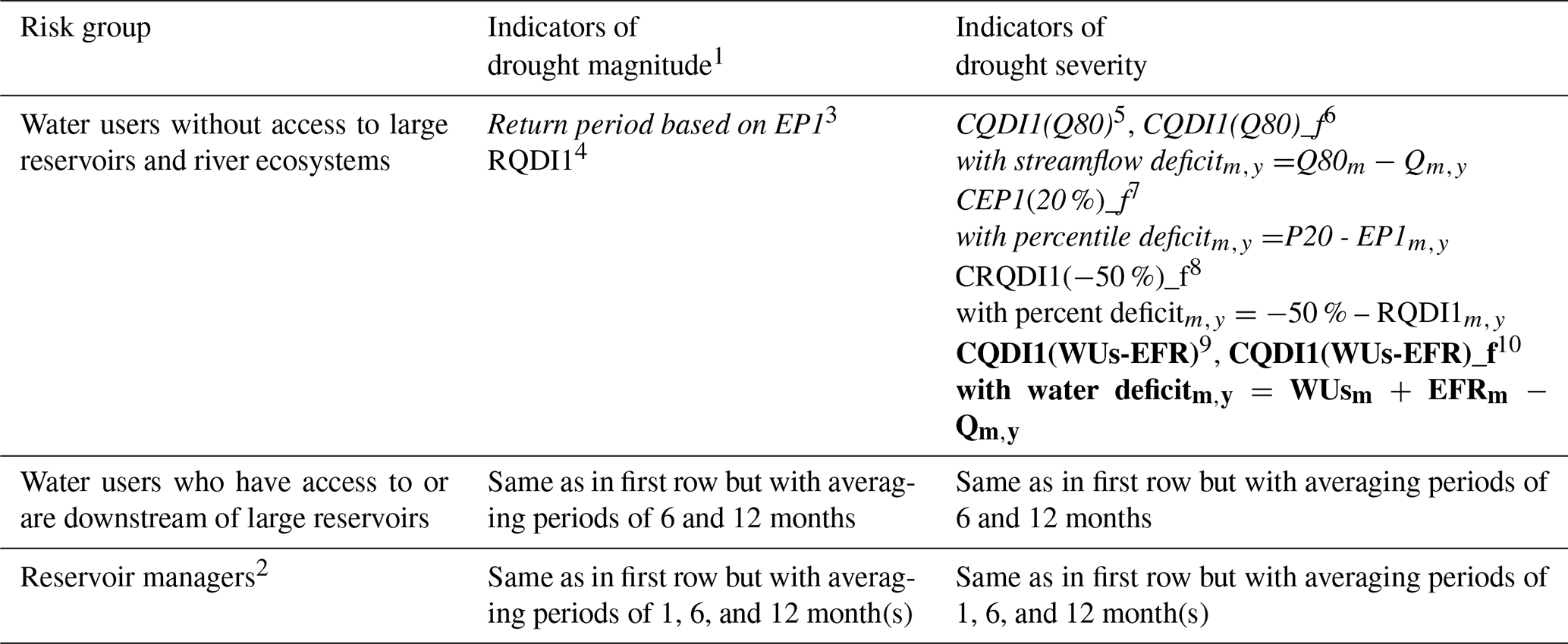
Table 1Characteristics of SDHIs suitable for global-scale assessments, classified according to inherent assumptions about habituation of people or other biota. The general terms “a certain degree” or “a certain reduction” in the first column are specified in a drought assessment by selected thresholds for drought definition.
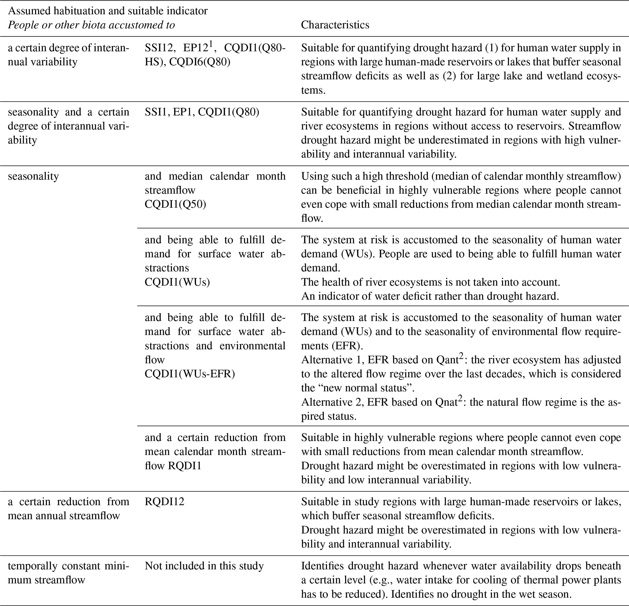
1 EP12: empirical streamflow percentile with an averaging period of 12 months (not analyzed in this study). 2 Qant, Qnat: modeled anthropogenic streamflow altered by human water use and human-made reservoirs (Qant); naturalized modeled streamflow (Qnat).
Percentile-based indicators including empirical streamflow percentiles, standardized indicators, and TLM indicators with a low streamflow percentile as a threshold are often applied in DEWSs (Bachmair et al., 2016; Cammalleri et al., 2016a). They are perceived as statistically consistent across different temporal and spatial scales, indicating the rarity of the event (Steinemann et al., 2015; WMO and GWP, 2016). Utilization of percentile-based indicators (e.g., SSI12, SSI1, and CQDI1(Q80) in Table 1) implies that people in different climate regions and social systems are equally habituated to a certain interannual variability, which is most likely not the case. The 20th streamflow percentile (or SSI1 = −0.84) would correspond to a low relative streamflow deviation (e.g., −20 %) in a humid region (low interannual variability) compared to a higher deviation (e.g., −50 %) in a semi-arid region (high interannual variability). Hence, percentile-based indicators might underestimate streamflow drought hazard in semi-arid areas where people (and ecosystems, although possibly to a lower degree) are often more vulnerable to reductions in water availability. Regions with high interannual variability are depicted in Fig. A1b. Here, drought hazard indicators that quantify relative deviations from the long-term mean or median (RQDI1, RQDI12 in Table 1) or TLM indicators with higher percentiles as a threshold (CQDI1(Q50) in Table 1) might be better suited to define drought conditions. Such indicators appear to be less preferred as periods with the same indicator value have different probabilities of occurrence in different regions and thus not the same rarity (Steinemann et al., 2015). Contrastingly, river ecosystems are, in the ideal case, perfectly adjusted to interannual variability of streamflow such that percentile-based drought hazard indicators are often suitable for drought hazard assessment for river ecosystems. In conclusion, percentile-based hazard indicators and relative deviations from the long-term mean or median should be used complementarily in large-scale DEWSs to cover different types of habituation.
The selected averaging period defines whether people are habituated to the annual or seasonal flow regime. One can assume that river ecosystems are generally accustomed to seasonality. Therefore, indicators with a short averaging period of, for example, 1 month (EP1, SSI1, RQDI1 and CQDI1 variants in Table 1) are appropriate for quantifying drought hazard for river ecosystems. Furthermore, short averaging periods are suitable in regions where farmers and other water users do not have access to large water storage such as reservoirs, lakes, or groundwater (either due to missing infrastructure or due to water use restrictions). As these users abstract water directly from the stream, they are very vulnerable to seasonal (monthly) streamflow deficits. Indicators with longer averaging periods (SSI12, RQDI12), on the other hand, are suitable in regions with large human-made reservoirs, which are usually replenished during the wet season such that streamflow deficits during the low-flow months are irrelevant. People in these regions are therefore only vulnerable to either interannual variability (SSI12) or mean annual conditions (RQDI12), but not to seasonality. Certainly, other averaging periods may be suitable depending on the region-specific storage capacity. Since volume-based indicators (TLM indicators) are also important components in water resources management (van Loon, 2015), the indicators CQDI1(Q80-HS) and CQDI6(Q80) are assessed as alternatives for SSI12 and RQDI12 (or rather the cumulated variants CSSI12 and CRQDI12) in regions with highly seasonal streamflow regimes (Fig. A1a) and large reservoirs.
For water managers, the status of the actual water deficit in terms of unsatisfied water demand might be as informative as the status of streamflow anomaly. Drought hazard is generally defined as a climate-induced anomaly, i.e., a period of below-normal water availability (McKee et al., 1993; van Lanen, 2006; van Loon, 2015). This concept can be broadened by assuming that a drought only occurs if the anomaly coincides with a water deficit for people or ecosystems (Cammalleri et al., 2016b; Popat and Döll, 2021; Wilhite and Glantz, 1985). Nevertheless, only a few studies exist wherein the combination of anomaly and deficit is translated into drought hazard indicators for soil moisture (Palmer, 1965; Cammalleri et al., 2016b; Popat and Döll, 2021) and streamflow (Popat and Döll, 2021). In the present study, the water deficit aspect of drought is represented by the indicators CQDI1(WUs) and CQDI1(WUs-EFR) (Table 1). Application of these indicators implies that the system at risk is habituated to the satisfaction of seasonal water demand. While CQDI1(WUs) neglects the water requirements of the ecosystem, CQDI1(WUs-EFR) assumes that the river ecosystem is habituated to the seasonality and magnitude of natural streamflow. As EFR might never be fulfilled in the case of strongly altered streamflow regimes, Qnat in the EFR computation can be replaced by Qant, implying that the river ecosystem has already adapted to the altered streamflow conditions (Table 1). Figure A1c shows regions where human water demand is high compared to available streamflow and where a drought hazard due to unsatisfied human surface water demand is likely.
3.2 Levels of drought characterization
Translating conceptual drought definitions into operational, quantitative drought hazard indicators is not straightforward due to the complexity of the underlying natural processes and the large number of indicators and methods that can be applied. In the literature, there is agreement about which drought characteristics are relevant for operational applications comprising the temporal component (onset, termination, duration) and the spatial extent as well as drought magnitude and severity, from which other metrics such as intensity, return period, and frequency or probability of occurrence can be derived (van Lanen et al., 2017). We understand drought magnitude as an anomaly or deficit occurring within a predefined period and severity as the accumulated deficit between the magnitude and a selected threshold since the onset of drought, which is defined by water availability dropping below the threshold (van Lanen et al., 2017). However, the terms drought magnitude and severity, which represent different levels of drought characterization, are not applied consistently in the literature. The terms are not made explicit and are sometimes interchanged (Steinemann et al., 2015; Vidal et al., 2010; López-Moreno et al., 2009). In particular, the commonly accepted classification of SDHIs into threshold-based and standardized indicators (van Loon, 2015) is somewhat misleading, since the former represents time series of severity and the latter time series of magnitude.
To facilitate a better understanding of the informative value of SDHIs, we suggest a new indicator classification that includes four types of indicators and distinguishes severity from magnitude indicators (Fig. 1). The indicator types (columns in Fig. 1) include the volume-based anomaly, the standardized or percentile-based anomaly, and the relative deviation (Sect. 2.3). Deficit anomaly indicators (last column in Fig. 1) combine an anomaly indicator with an indicator of the deficit with respect to optimal water availability (e.g., Popat and Döll, 2021). For each indicator type, two levels of drought characterization, drought magnitude (level 1) and severity (level 2), can be computed.
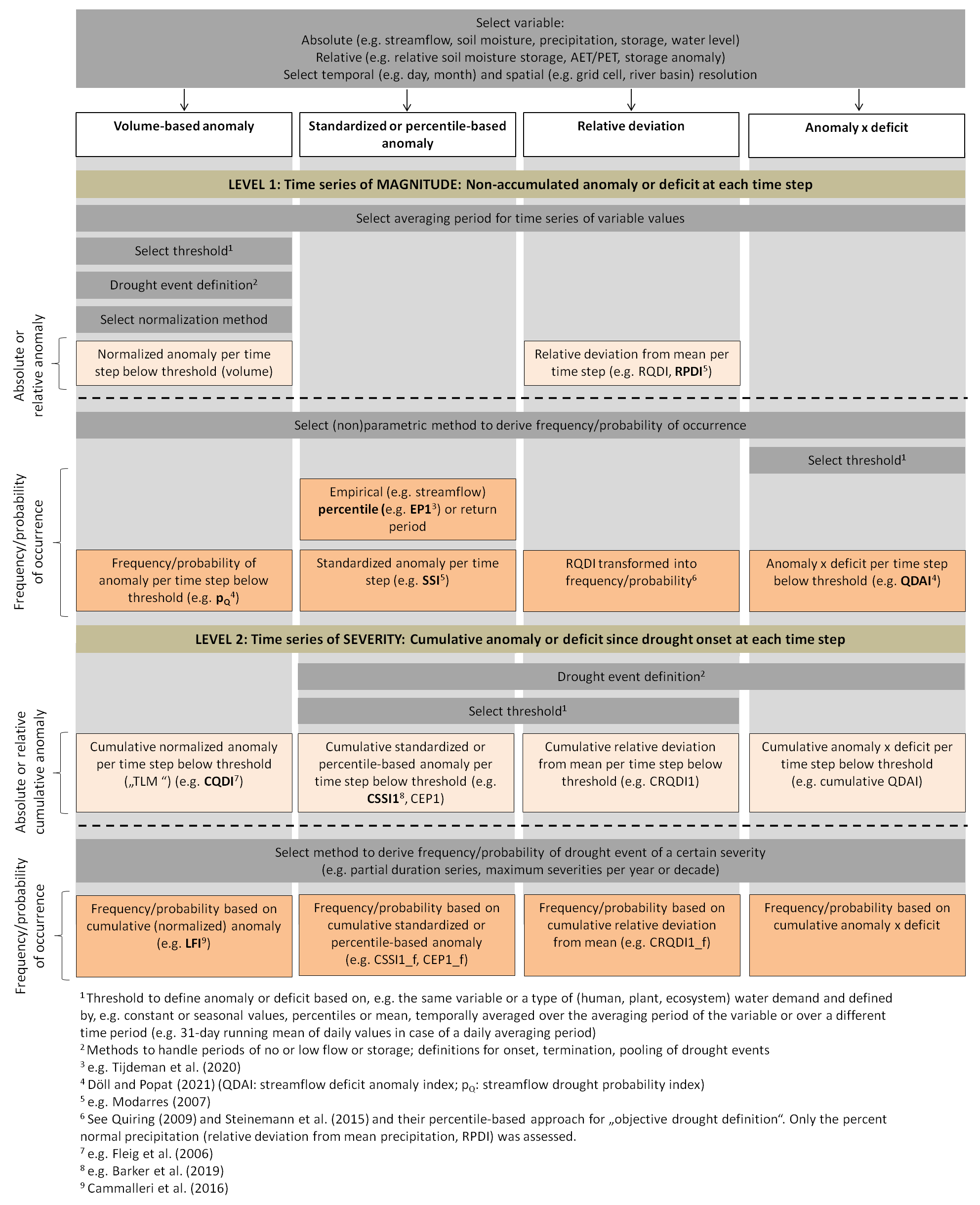
Figure 1Classification system including four types of drought hazard indicators, indicating (1) the magnitude of the drought at a certain time step as a deficit and/or anomaly (level 1) or (2) the severity of the drought event, i.e., the cumulative magnitude of drought since drought onset (level 2). Both magnitude and severity can be expressed in terms of frequency or probability to compare the drought of interest to other droughts. The dark grey boxes indicate decisions that have to be made when computing the indicators, e.g., which averaging period is selected. Indicators in bold have already been applied in the literature. Assumptions about the habituation of people and ecosystems determine the selection of the type of indicator, the averaging period, and the threshold (see Table 1).
The dark grey boxes in Fig. 1 represent decisions regarding time step length and averaging period, as well as drought threshold and definition of drought events (minimum length of drought event, pooling of drought events). These decisions depend on the assumed habituation of people and ecosystems to certain streamflow conditions (Sect. 3.1 and Table 1). Beige and orange boxes contain indicators that are expressed in absolute or relative values and in frequency or probability of occurrence, respectively. Indicators applied in drought monitoring (CQDI1, low-flow index – LFI, percentiles, SSI, RDPI) or in the literature (pQ, cumulative SSI, streamflow deficit anomaly indicator QDAI) are written in bold. The units of the four indicator types differ at both level 1 and 2, but indicators can be directly compared when expressed in units of probability (or frequency) of non-exceedance.
Figure 1 shows that drought hazard indicators pertaining to one of the four indicator types can be transformed between level 1 (magnitude) and level 2 (severity) while still sharing the type-specific conceptual drought definition. Furthermore, the classification system clarifies that each indicator type requires a threshold setting either at level 1 or 2. Hence, the term “threshold-based” applies to any indicator of drought severity, and it is therefore not a suitable criterion for distinguishing types of indicators.
The differentiation of indicator types can be ambiguous. For instance, standardized and percentile-based anomaly indicators are subsumed in Fig. 1 (column 2), although there is a minor conceptual difference between them as highlighted by Tijdeman et al. (2020). While standardized indicators show the non-exceedance probability enabling extrapolation, empirical percentiles represent the historical non-exceedance frequency within the boundaries of observations. We account for this aspect by including the terms frequency and probability in Fig. 1.
On the other hand, volume-based and standardized or percentile-based anomaly indicators are presented as different indicator types, although they can be based on the same conceptual drought definition if equivalent thresholds are applied. If Q80 is used as a threshold for CQDI1 and −0.84 for cumulative SSI1 (corresponding to the 20th percentile for cumulative EP1 and a return period of 5 years), both indicators capture the same drought signal. Differences between the drought signals are then attributable to the computational methods for the standardization of streamflow. Analyzing the sensitivity of SSI1 to different parametric and nonparametric standardization methods in European river basins, Tijdeman et al. (2020) revealed considerable differences in computed SSI1 among seven probability distributions (and two fitting methods) and five nonparametric methods. A major difference between volume-based and standardized indicators is that the former detect absolute drought deficits and the latter relative drought deficits. This can result in different frequency values for the same drought event.
The objective of this section is to identify which of the SDHIs presented in Table 1 can be meaningfully quantified at the global scale using WaterGAP 2.2d and which SDHIs are appropriate for monitoring different drought hazards in large-scale DEWSs. We emphasize that the objective is not a drought impact assessment, which is beyond the scope of this study. We want to show how the conceptual discrepancies and similarities between SDHIs (Sect. 3), which are of a general nature and apply to any month of the reference period, are translated into global-scale hazard indicators and how these indicators should be interpreted by end users of a large-scale DEWS. The indicators are illustrated in global maps for 2 example months capturing known drought events in Europe (July 2003) and South Africa (September 1993), two regions that are characterized by different streamflow regimes and assumed habituation. Following the classification of Table 1, SDHIs are differentiated by drought magnitude (Figs. 2 and S3) and drought severity, the latter either expressed as volume-based anomaly or deficit (Figs. 3 and S4) or as frequency of non-exceedance (denoted with the suffix “_f”) (Figs. 5 and S5). In addition, CQDI1(Q80) and CQDI1(Q80-HS) are compared at the global scale with respect to drought occurrence during the whole reference period (Fig. 4). SDHIs are further illustrated for four selected gauging stations with different streamflow regimes and assumed vulnerabilities of the risk system to streamflow anomalies (Figs. 6, S2, and S6). These include two stations with low interannual streamflow variability (Danube River at Hofkirchen, Germany, with probably low vulnerability and Angara River at Boguchany, Russia, with possibly higher vulnerability) and two stations with high interannual variability (White River near Oacoma, US, with probably low vulnerability and Orange River at Vioolsdrif, South Africa, with possibly higher vulnerability).
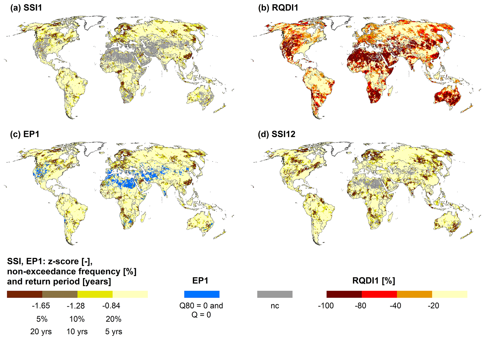
Figure 2Magnitude of drought hazard (level 1 in Fig. 1): non-cumulative anomaly in July 2003 as indicated by SSI1 (a), RQDI1 (b), EP1 (c), and SSI12 (d) for the reference period 1986–2015. For the standardized indicators and EP1, the z scores and the corresponding frequencies of non-exceedance and return periods are shown. In the blue grid cells in (c), drought identification is not possible with EP1, since Q80 and Q are zero. The notation “nc” indicates not computable.
4.1 SDHIs based on empirical percentiles or standardized streamflow
EP1 patterns (Fig. 2c for July 2003 and Fig. S3c for September 1993) are very similar to SSI1 (Fig. 2a and S3a) since both indicators are based on the same conceptual drought definition (Sect. 3.1). Both indicators generally identify the same drought regions. However, drought classes differ in many regions of the world, with EP1 indicating both higher and lower drought magnitude. For instance, in eastern France, EP1 indicates a higher drought magnitude class in July 2003 (return period RP > 20 years) than SSI1 (RP > 10 years) and vice versa in southern Germany. In September 1993, SSI1 indicates a higher drought hazard than EP1 for the Orange River along the Namibia–South Africa border, but a lower hazard in a few grid cells in central South Africa and Lesotho. These differences can be attributed to the fitting of the gamma distribution in the case of SSI1 and the assignment of the maximum rank among tied values within a streamflow sample in the case of EP1 (Sect. 2.3.3).
Comparing SSI1 with empirical percentiles, Tijdeman et al. (2020) identified several advantages and limitations for both indicators. SSI1 has the disadvantage that for different streamflow regimes, different parametric probability distributions would be required to achieve the best fit, which reduces consistency at the global scale. In this study, the gamma distribution showed the best fit among 23 parametric probability distributions for most grid cells and was applied in each month and grid cell. Of course, using only one distribution for the whole globe results in poorly fitting distributions for some cells and months (Tijdeman et al., 2020). Grid cells where gamma fitting was rejected in the calendar months July and September based on the KS test (Sect. 2.3.1) are shown in grey in Figs. 2a and S3a (18 % of all grid cells excluding Greenland). EP1 does not require fitting of a distribution and can therefore be computed in more grid cells than SSI1. Only if a sample includes more zero flows than the selected threshold is drought identification not possible (blue grid cells in Figs. 2c). On the other hand, if Q80 is zero and the current streamflow exceeds zero, it is possible to define the current month as not a drought month (shown in beige in Fig. 2a and c). EP1 has the disadvantage that it only allows the quantification of the historical non-exceedance frequency within the reference period, while probabilistic information, for example on extreme events such as a 100-year drought, cannot be derived (Tijdeman et al., 2020). Nonetheless, EP1 seems to be more suitable for a global-scale DEWS, as the indicator does not entail the possibly large uncertainties due to the fitting of a probability distribution and can be computed in more grid cells than SSI1.
4.2 SDHIs assuming habituation to mean streamflow or interannual variability of streamflow
With percentile-based indicators (e.g., EP1, SSI1), risk systems in different regions are assumed to be equally habituated to a certain interannual streamflow variability, which is most likely not the case as interannual variability varies strongly (Fig. A1b). Comparing two regions with high and low interannual variability, the same streamflow percentile or z score corresponds to a much higher relative deviation from mean calendar month streamflow (RQDI1) if interannual variability is high. For instance, at the Orange River and White River with high interannual variability (Fig. S2), SSI1 values below −0.84 (RP > 5 years) always correspond to RQDI1 values below −70 % and −60 %, respectively. At the Danube River and Angara River (Fig. S2) (low interannual variability), RQDI1 of −50 % is (almost) never reached, while maximum SSI1 values are higher than at the Orange River and White River. Hence, SSI1 might underestimate drought magnitude if interannual variability is high, especially for vulnerable systems.
At the global scale, RQDI1 (Figs. 2b and S3b) identifies most of the drought hotspots as indicated by EP1 (Figs. 2c and S3c), although the relative levels of magnitude differ. These differences correspond well to the interannual streamflow variability depicted in Fig. A1b. Drought hotspots according to EP1 in regions with low interannual variability (parts of North America, northern Europe, northern Russia) only show moderate relative streamflow deviations by global comparison. This is because RQDI1 values of −50 % or lower are never reached in these regions, as illustrated at the Danube and Angara stations (see above). Here, RQDI1 might underestimate drought magnitude. On the other hand, in regions with high interannual variability (e.g., large parts of Africa, central Asia, western US), both drought magnitude and the affected area are larger according to RQDI1. Here, RQDI1 can draw attention to potential drought impacts in regions with higher suspected vulnerability (e.g., southern Africa) that would otherwise be overlooked using EP1 or SSI1. In regions where people are probably well accustomed to the interannual variability of streamflow (e.g., western US), RQDI1 is less suited than EP1 to indicate drought magnitude. At the severity level, regions with low interannual variability are excluded using CRQDI1(−50 %)_f (Figs. 4d and S5d) due to the low threshold of −50 % (grid cells in light grey).
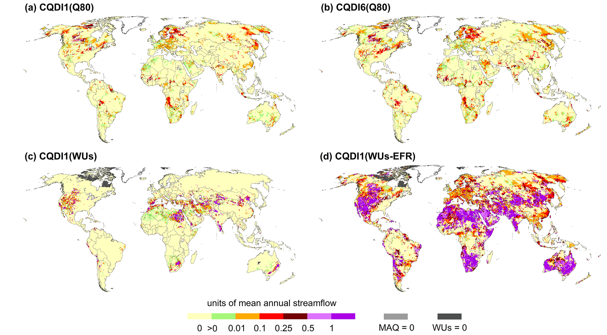
Figure 3Severity of drought hazard (level 2 in Fig. 1): cumulative deficit in July 2003 since the onset of a drought event as indicated by CQDI1(Q80) (a), CQDI6(Q80) (b), CQDI1(WUs) (c), and CQDI1(WUs-EFR) (d) for the reference period 1986–2015. Grid cells with a deficit of zero are shown in beige. Values larger than zero and below 0.1 are shown in green. A value of 0.1, for example, denotes that the current cumulative deficit is equivalent to 10 % of mean annual streamflow (MAQ). WUs: mean annual surface water withdrawals.
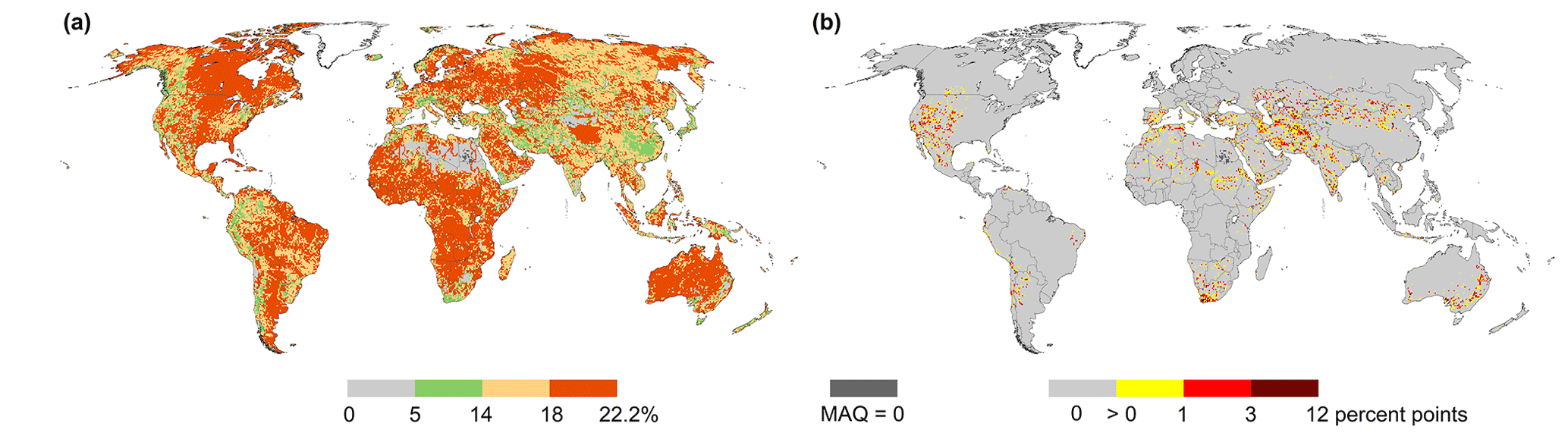
Figure 4Comparison of CQDI1(Q80) and CQDI1(Q80-HS) in the reference period 1986–2015: percent of months in drought based on CQDI1(Q80) (a) and the increase due to the “HS method” in percent points (b). Both indicators allow an existing drought to continue in months in which Q80 and the current streamflow Q are zero. The HS method additionally facilitates drought prolongation in months with Q80 = 0 if Q>0. Neither indicator allows a drought to begin in months with Q80 = 0. Drought prolongation in the case of Q80 = 0 is only possible if a streamflow deficit was computed in at least 2 antecedent months with Q80 >0 (2mc, Sect. 2.3.2). In (a), the fraction of drought months is reduced to <20 % if 1-month droughts are ignored (2mc). In grid cells with 0 % in (a), Q80 is either always zero, or the few calendar months with Q80 > 0 result in 1-month droughts only. The fraction can be increased to > 20 % in the case of drought pooling (2mc) or in the case of drought prolongation if Q80 = 0. MAQ: mean annual streamflow.
4.3 SDHIs taking into account human water use and EFR
The water deficit indicators CQDI1(WUs) and CQDI1(WUs-EFR) (Figs. 3c, d and S4c, d) define drought as “less water than needed” as opposed to the anomaly indicator CQDI1(Q80) (Figs. 3a and S4a) indicating “less water than normal” (or rather less water in a certain month than in 80% of the years). Consequently, the spatial pattern of the former is very different from CQDI1(Q80) patterns. For instance, the drought event in 2003 in central and eastern Europe (Fig. 3) identified by CQDI1(Q80) is not indicated by CQDI1(WUs), while the latter shows an additional drought hazard in the northern part of South Africa (Fig. S4). This is because CQDI1(WUs) strongly depends on surface water stress, which is generally low in Europe and high in South Africa (Fig. A1c). The spatial patterns of CQDI1(WUs) correlate well with Fig. A1c, comparing human water demand for surface water as a fraction of mean streamflow. CQDI1(WUs-EFR) additionally considers the environmental flow requirement (EFR) computed as 80% of naturalized mean calendar month streamflow. Like RQDI1, the indicator thus depends on mean monthly streamflow, and the spatial pattern corresponds well to the map of interannual variability (Fig. A1b). A comparison between CQDI1(WUs) and CQDI1(WUs-EFR) shows that only in a few regions is human water demand the dominant component determining the water deficit. In most regions, EFR leads to high cumulative deficits even if seasonal human water demand is small (< 10 % of available streamflow, Fig. A1c). CQDI1(WUs-EFR) is the only indicator in this study that explicitly takes into account the health of the river ecosystem, an aspect that should be included in a global-scale DEWS. Alternatively, the cumulative anomaly deficit indicator (QDAI) (Popat and Döll, 2021), considering EFR based on a similar approach, can inform decision-makers and water users about the drought hazard for water supply. In strongly altered flow regimes, wherein simulated anthropogenic monthly streamflow (Qant) is always below 80 % of mean monthly naturalized streamflow (Qnat), time series of CQDI1(WUs-EFR) are continuously increasing, and it is not possible to distinguish drought events. In such cases, it is more meaningful to set EFR to 80 % of mean monthly Qant, implying that the altered flow regime is the “new normal” (see also Table 1).
4.4 SDHIs for reservoir management or water users with access to reservoirs
In large-scale hydrological modeling, it is very difficult to accurately simulate how human-made reservoirs affect water availability, i.e., how they impact downstream streamflow and how reservoir storage varies in time. Therefore, it is more informative to use time series of reservoir inflow (streamflow data) instead of reservoir storage for assessing drought hazard for these risk systems. For water users that depend on large reservoirs, streamflow deficits during the low-flow months are not relevant, since reservoirs can store water from the high-flow season. Hence, drought magnitude should be assessed using SDHIs with longer averaging periods that either assume habituation to interannual variability (e.g., SSI12, EP12, Table 1) or mean annual conditions (RQDI12, Table 1), but not seasonality. At the four investigated gauging stations (Fig. S2), the relation between SSI12 and RQDI12 is the same as for SSI1 and RQDI1 (Sect. 4.2). If interannual variability is high (Orange River and White River), SSI12 values correspond to much higher RQDI12 values compared to the stations with low interannual variability (Danube River and Angara River). To obtain drought severity, these indicators can be cumulated using a suitable threshold. As described in Sect. 4.2, a threshold of −50 % for RQDI12 would exclude regions with low interannual variability, where this value is rarely reached, and where RQDI12 might underestimate drought magnitude.
In addition to these magnitude indicators, the volume-based severity indicators CQDI1(Q80-HS) and CQDI6(Q80) were assessed. With CQDI1(Q80-HS), an existing drought is allowed to continue in months in which the calendar month Q80 is zero, even if streamflow Q exceeds zero. In contrast, CQDI1(Q80) only allows a drought to continue if Q80 and Q are zero. A comparison of the two indicators (Fig. 4) reveals that the impact of the HS method is rather small at the global scale but can be relevant at the regional scale. Figure 4a depicts the fraction of drought months as a percentage of all 360 months during the reference period as indicated by CQDI1(Q80). Using Q80 as a threshold implies that the time series should be in drought 20 % of the time. The fact that this percentage is often reduced and sometimes increased can be attributed to the 2-month criterion (Sect. 2.3.2) (1-month droughts are ignored, and several droughts are pooled) and to drought prolongation if Q80 and Q are zero. The HS method leads to an increase in drought months by up to 3 percent points (corresponding to 11 out of 360 months) in 6 % of all grid cells, e.g., parts of India, Pakistan, Afghanistan, Iran, and the western US, all of which are regions with highly seasonal streamflow regimes (Fig. 4b). Larger increases of up to 12 percent points are only computed in 0.4 % of all grid cells. Hence, the additional information value of CQDI1(Q80-HS) in a large-scale DEWS would be small. Instead, CQDI variants with longer averaging periods like CQDI6(Q80) (Figs. 3b and S4b) are more suitable for assessing risk systems with reservoirs. The time series of CQDI6(Q80) at the four gauging stations (Fig. S2) illustrate how the maximum drought severity is shifted by 1 month or more compared to CQDI1(Q80), reflecting the fact that a reservoir storage requires several months of “normal” streamflow to be replenished.
4.5 Range of drought severity as quantified by the various SDHIs
A direct comparison between different severity indicators is possible when the time series of drought severity are transformed into frequency of non-exceedance. Figures 5 and S5 depict the probability (frequency) of non-exceedance p of drought severity in July 2003 and September 1993, respectively, between four CQDI1 variants, the cumulative relative deviation CRQDI1 with a threshold of −50 %, and the cumulative empirical percentile CEP1 with a threshold of 20 %. The indicators are denoted with the suffix “f” for frequency. A p value of 0.7, for example, indicates a high drought hazard, with the severity up to July 2003 being higher than the severity of 70 % of all completed drought events in the reference period. In both example months, the spatial extent of regions with p>0.7, i.e., severe droughts, is larger according to the indicators that do not assume habituation to interannual variability (CQDI1(Q50)_f, CQDI1(WUs)_EFR_f, and CRQDI1(−50 %)_f). Spatial patterns of CQDI1(Q50)_f and CQDI1(WUs-EFR)_f are rather similar. Correspondence between these two indicators is higher than between CQDI1(Q50)_f and CQDI1(Q80)_f. CRQDI1(−50 %)_f identifies fewer regions with severe drought status compared to CQDI1(Q50)_f but more regions compared to CQDI1(Q80)_f.
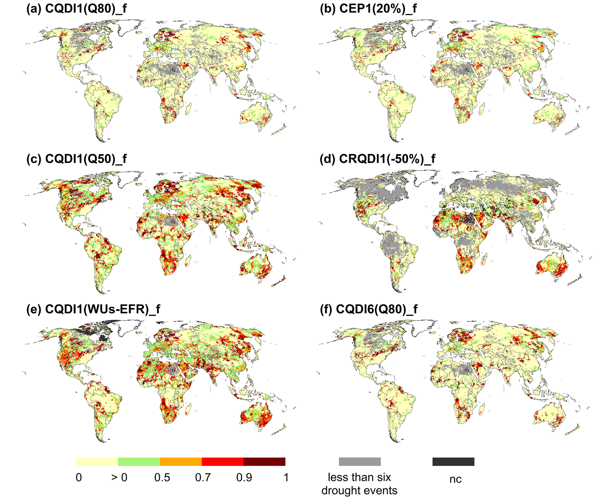
Figure 5Probability of non-exceedance of drought events (level 2 in Fig. 1) in July 2003 for the cumulative indicators CQDI1(Q80)_f (a), CEP1(20 %)_f (b), CQDI1(Q50)_f (c), CRQDI1(−50 %)_f (d), CQDI1(WUs-EFR)_f (e), and CQDI6(Q80)_f (f) for the reference period 1986–2015. A value of 0.8, for example, indicates that the cumulative anomaly or deficit, i.e., the severity up to this month, is higher than the severity of 80 % of all drought events in the reference period. The probability of non-exceedance was not computed for grid cells shown in light grey, where fewer than six drought events were computed in the reference period (Sect. 2.4). The notation “nc” stands for “not computable”.
Spatial patterns of CQDI1(Q80)_f (Figs. 5a and S5a) and CEP1(20 %)_f (Figs. 5b and S5b) are very similar, since they are based on the same drought concept. Nonetheless, small differences occur in all identified drought hotspots, which can be explained by the fact that the former quantifies absolute and the latter relative streamflow anomalies per calendar month, leading to a different ranking of low-flow and high-flow droughts during the reference period. This relation is illustrated for the Danube gauging station in Fig. 6 and for the other three investigated stations in Fig. S6. Although CEP1(20 %) (in units of cumulative percent) and CQDI1(Q80) (in units of mean annual streamflow) capture the same drought signal at the four stations, the relative levels among the drought events differ. In Fig. 6, the three most severe droughts according to CQDI1(Q80) are the drought events in 1998, followed by 2014 and 2003. In contrast, the 2003 drought, which occurred mainly during the low-flow period (August to November), has the second-highest severity according to CEP1(20 %). The high-flow drought from March to May 2011, on the other hand, has a lower severity rank according to CEP1(20 %). The differences are more pronounced with higher seasonal variability (Orange River and White River, Fig. S6) but almost negligible if seasonality is very low (Angara River, Fig. S6). Consequently, in a large-scale DEWS, CEP1(20 %) appears to be more suitable in regions where the risk system is more vulnerable to low-flow droughts than to high-flow droughts. These differences would not occur if volume-based monthly streamflow deficits were normalized using mean monthly streamflow. They only occur if they are either not normalized (e.g., the low-flow index – LFI, Cammalleri et al., 2016a) or normalized against mean annual streamflow volume (e.g., van Loon et al., 2014, and all CQDI1 variants in this paper).
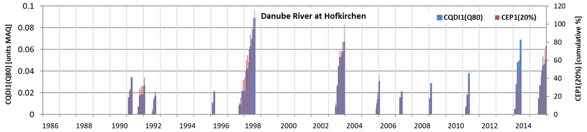
Figure 6Drought severity per month during the reference period 1986–2015 at the Danube River, Hofkirchen, Germany, as indicated by CQDI1(Q80) (blue) and CEP1(20 %) (red). MAQ: mean annual streamflow.
Continental and global DEWSs, which encompass near-real-time monitoring as well as seasonal forecasts, aim to provide information about drought hazards for diverse risk systems, which are characterized by different risk bearers (e.g., human water supply, river ecosystems), habituation, streamflow regimes, and water storage capacities. Therefore, a large-scale DEWS should provide data for a rather large number of drought hazard indicators together with a clear description of suitability for different risk systems including the underlying assumptions about habituation (or adaptation) of the risk bearer to the streamflow regime (Sect. 3.1). Then, end users can select and combine several drought hazard indicators that are most informative. Table 2 lists the SDHIs that should be provided by large-scale DEWSs, differentiating three risk groups and three main types of habituation. In a DEWS, drought magnitude indicators should be clearly differentiated from drought severity indicators (Sect. 3.2), and the specific suitability of each SDHI for different risk systems should be explained comprehensively.
Table 2SDHIs for human water supply and river ecosystems that should be provided by large-scale DEWSs for different risk groups. Italic font: indicator assumes habituation to a certain degree of interannual variability (see Fig. A1b). Bold font: indicator assumes the ability to fulfill seasonally varying demand for surface water abstractions and environmental flow. Normal font: indicator assumes habituation to a certain reduction from mean monthly streamflow, and it is likely suitable for highly vulnerable systems with high interannual streamflow variability. All indicators assume habituation to the seasonality of streamflow.
1 In regions with (suspected) poor quality of hydrological model output, analysis of SPEI6 and SPEI12 is suggested in addition to SDHIs. 2 Reservoir managers should be informed to consider SDHIs of the grid cells that represent inflow into the reservoir. 3 EP1: empirical streamflow percentile per calendar month with an averaging period of 1 month, with 0< EP1 ≤ 100 %. EP1 expresses the frequency of non-exceedance of the current streamflow. The return period, in years, is computed as 100 EP1. The lower the EP1 and the higher the return period, the higher the drought hazard. 4 RQDI1: relative deviation of monthly streamflow from mean calendar month streamflow (MMQ) in percent. It is calculated as the difference between monthly streamflow and the respective MMQ, which is then divided by MMQ. The indicator is not computable in months with MMQ = 0. 5 CQDI1(Q80): cumulative volume-based streamflow deficit with an averaging period of 1 month divided by mean annual streamflow. A deficit occurs if monthly streamflow Qm,y falls below Q80m (the 20th percentile) of the long-term calendar month streamflow. Monthly deficits are accumulated for all drought months to obtain severity. A drought event starts with at least 2 consecutive months with a deficit, and it ends (deficit set to zero) if there are 2 consecutive months without a deficit (2mc: 2-month criterion). Any streamflow surplus over Q80 in a single month between 2 deficit months does not decrease the cumulative deficit. To address flow intermittency, an existing drought continues during months in which both Q80 and the current streamflow are zero. If Q80 = 0 and the current streamflow exceeds zero, the drought event ends. Hence, a drought can be prolonged, but never begin, in calendar months with Q80 = 0. The indicator is expressed in units of mean annual streamflow. 6 CQDI1(Q80)_f: the frequency of non-exceedance of drought events of a certain severity as quantified by CQDI1(Q80), with values between 0 and 1. A high frequency value indicates a high drought hazard. First, the partial duration series of drought events is derived based on the severities of all drought events of the reference period. Grid cells with fewer than six drought events are excluded. Second, the frequency of non-exceedance is quantified using the exponential cumulative distribution function. Preferably, the indicator should be expressed as the return period Tr= 1/(θ(1-CQDI1(Q80)_f)), with θ as the average number of drought events per year during the reference period. 7 CEP1(20 %)_f: the frequency of non-exceedance of drought events of a certain severity (see above) as quantified by the cumulative percentile-based anomaly CEP1(20 %). The monthly percentile deficit is computed by subtracting the current streamflow percentile EP1m,y from the percentile threshold P20. Like CQDI1(Q80), CEP1(20 %) allows an existing drought event to continue during months in which both Q80 and the current streamflow are zero. The 2mc is also applied. As the unit of CEP1(20 %) (cumulative percent) is not informative, the indicator should be provided in frequency of non-exceedance or preferably as the return period Tr=1/(θ(1-CEP1(20 %)_f)), with θ as the average number of drought events per year during the reference period. 8 CRQDI1(−50 %)_f: the frequency of non-exceedance of drought events of a certain severity (see above) as quantified by the cumulative relative streamflow deviation CRQDI1(−50 %). The monthly percentile deficit is computed by subtracting the relative deviation of the current month RQDI1m,y from the threshold −50 %. Months with MMQ = 0, for which the relative deviation is not computable, are defined to end a drought event assuming that people are habituated to zero streamflow in this month. The 2mc is also applied. As the unit of CRQDI1(−50 %) (cumulative percent) is not informative, the indicator should be provided in frequency of non-exceedance or preferably the return period Tr= 1/(θ(1-CRQDI1(−50 %)_f)), with θ as the average number of drought events per year during the reference period. 9 CQDI1(WUs-EFR): cumulative, volume-based water deficit with an averaging period of 1 month divided by mean annual streamflow. It is computed like CQDI1(Q80) but using the threshold mean monthly potential surface water abstraction WUsm plus environmental flow requirement (EFRm) per calendar month. EFR is assumed to be 80 % of mean monthly naturalized streamflow Qnat per calendar month. As EFR might never be fulfilled in the case of strongly altered streamflow regimes, Qnat can be replaced by Qant, implying that the river ecosystem has adapted to the altered streamflow conditions. WUs represents the water demand from surface water bodies. The indicator is not computed in grid cells where mean annual WUs in the reference period is zero (approx. 9 % of all grid cells excluding Greenland). The indicator is expressed in units of mean annual streamflow. 10 CQDI1(WUs-EFR)_f: the frequency of non-exceedance of drought events of a certain severity (see above) as quantified by CQDI1(WUs-EFR). The indicator should be expressed as the return period Tr = 1/(θ(1-CQDI1(WUs-EFR)_f)), with θ as the average number of drought events per year during the reference period.
To assess drought magnitude, we recommend using empirical percentiles and relative deviations to cover risk systems that are either habituated to a certain degree of interannual variability or to a certain reduction to mean calendar month streamflow. An averaging period of 1 month is suitable for river ecosystems and water users without access to large reservoirs, who depend on the currently available streamflow. Longer averaging periods of 6 or 12 months are suitable for people who have access to or are downstream of reservoirs that are replenished during high-flow periods and that can alleviate short periods of below-normal streamflow. For reservoir managers, EP and RQDI with short and longer averaging periods (1, 6, and 12 months) are recommended for monitoring current reservoir inflow anomalies as well as reservoir storage anomalies (with different averaging periods depending on the storage capacity of the reservoir). Due to model uncertainties, time series of reservoir storage as simulated by WaterGAP should not be used for drought assessment. Importantly, reservoir managers should only consider SDHIs of the grid cells that represent inflow into the reservoir. This also applies if drought hazard for large lakes is analyzed by SHDIs.
We favor empirical percentiles (EP) over SSI as the former are more transparent to end users of a DEWS and do not entail uncertainties due to the fitting of a probability distribution. Moreover, application of one selected probability distribution function at large scales will always exclude many grid cells where the fitting is not possible. Here, other methods such as empirical percentiles would be required in any case. Expressing percentiles as a return period (in years) may further increase the transparency of EP as end users are accustomed to quantifying flood hazards by return periods. If the current streamflow is lower than the 30 values of the reference period, EP would only indicate a return period > 30 years (or a z score below −1.83), while SSI would indicate an extrapolated value, albeit with high uncertainty (Tijdeman et al., 2020). Hence, 40 reference years should be used, if possible, to differentiate severe and extreme droughts with return periods of up to 40 years (equivalent to ). In addition to the streamflow-based indicators, the standardized precipitation–potential evapotranspiration index (SPEI) (Vicente-Serrano et al., 2010) is suggested in regions with (suspected) poor quality of hydrological model output. Longer averaging periods of 6 and 12 months are recommended to consider the delayed response of streamflow to below-normal precipitation and potential evapotranspiration. However, it should be noted that meteorological indicators have limitations in describing hydrological drought processes (Haslinger et al., 2014; Blauhut et al., 2016; Laaha et al., 2017).
Drought severity should be assessed with indicators that imply habituation to a certain degree of interannual variability (CEP(20 %) and CQDI(Q80)), to a certain reduction from mean monthly streamflow (CRQDI(−50 %)), and to the ability to fulfill seasonally varying human water demand from surface water and environmental flow (CQDI(WUs-EFR)). Recommended averaging periods are the same as for magnitude indicators. With exceptions, we recommend that drought severity at a certain point in time be expressed in terms of the probability or frequency of non-exceedance (return period) of a drought event with such severity. These recommendations also relate to variable types other than streamflow (precipitation, soil moisture, etc.) and other spatial scales. In addition, the CQDIs should be provided in units of mean annual streamflow. CRQDI1(−50 %) is preferred over CQDI1(Q50), which is based on a similar assumption about habituation since percent deviations are often applied in climate change impact studies and may thus be easier to grasp. Moreover, CQDI1(WUs-EFR) is preferred over CQDI1(WUs) since the environmental component of water demand should be considered in a DEWS. Regarding the percentile-based indicators CEP1(20 %) and CQDI1(Q80 %), the problem of flow intermittency is overcome by allowing an existing drought to continue during months in which Q80 and the current streamflow are zero. CEP1 was found to be more sensitive to low-flow droughts than CQDI1, and it is therefore preferred over the latter if the risk system is more vulnerable to low-flow droughts than to high-flow droughts. CQDI1(Q80-HS), conceptualized for risk systems with reservoirs, is not recommended due to the small impact of the HS criterion (Sect. 2.3.2) at the global scale.
According to Stahl et al. (2020), practitioners often use particular streamflow values rather than anomalies as the trigger for management actions. These practitioners could use forecasted RQDI1 as provided by the global-scale DEWS to determine whether this trigger will be reached by computing streamflow from RQDI1 and observed mean monthly streamflow.
This paper presents a new systematic approach for selecting global-scale streamflow drought hazard indicators (SDHIs) for monitoring drought hazard for human water supply and river ecosystems in large-scale drought early warning systems (DEWSs). The methodology replaces the conventional and imprecise classification into threshold-based and standardized indicators by a new classification scheme that distinguishes indicators pertaining to four indicator types by (a) their inherent assumptions about the habituation of people and the ecosystem to the streamflow regime and (b) their level of drought characterization, namely drought magnitude and drought severity. The new scheme facilitates a better understanding of the information value of drought hazard indicators. It can support the development of a (large-scale) DEWS as well as water managers who rely on drought hazard indicators for their decision-making.
When providing drought hazard information in a global- or continental-scale DEWS, it is unknown which streamflow characteristics people and river ecosystems are locally accustomed to, and it is uncertain to what degree people have access to water stored in reservoirs. The suitability of hazard indicators is region- and risk-system-specific (Blauhut et al., 2022) and can only be evaluated with local knowledge about the vulnerability of the system at risk. Therefore, a large-scale DEWS should provide data for a rather large number of drought hazard indicators that characterize the condition of various water flows (streamflow, actual evapotranspiration as a fraction of potential evapotranspiration) and water storage compartments (snow, soil, groundwater, lakes). Clear explanations for the end users about the suitability of drought hazard indicators for specific risk systems need to be provided in DEWSs. When selecting hazard indicators, we recommend that end users make their assumptions about the habituation of the risk bearer explicit before selecting a drought hazard indicator that fits these assumptions. We suggest that future studies analyze how well these hazard indicators, in combination with suitable vulnerability and exposure indicators, can estimate drought impacts in the targeted risk systems at regional or national scales.
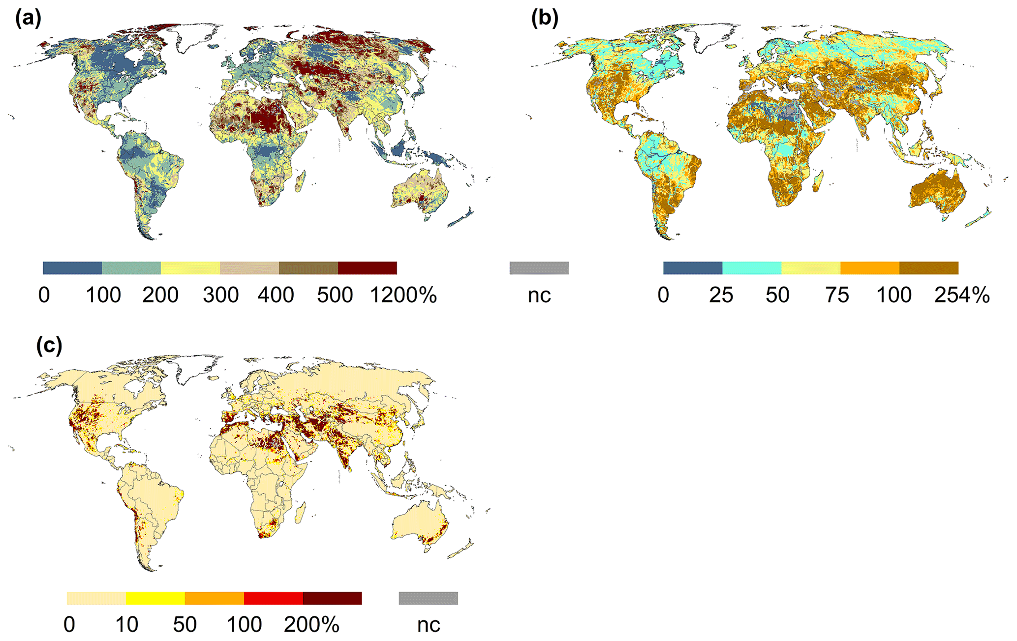
Figure A1Seasonal streamflow variability indicated by the seasonal amplitude (Q in calendar month with highest mean monthly Q minus Q in calendar month with lowest mean monthly Q divided by MMQ – mean monthly Q over all calendar months) (a), interannual streamflow variability indicated by the average of the 12 calendar month values of (Q20–Q80) Qmean (b), and average of the 12 calendar month values of WUsmean Qmean (c). All values in percent.
WaterGAP 2.2d model output data used in this study are available at https://doi.org/10.1594/PANGAEA.918447 (Müller Schmied et al., 2020). The WaterGAP 2.2d source code is published at https://doi.org/10.5281/zenodo.6902111 (Müller Schmied et al., 2022). The outputs from this study are available at https://doi.org/10.5281/zenodo.7764879 (Herbert and Döll, 2023). GRDC monthly streamflow data are available at https://portal.grdc.bafg.de/applications/public.html?publicuser=PublicUser#dataDownload/Home (GRDC, 2019; last access: 6 June 2023).
The supplement related to this article is available online at: https://doi.org/10.5194/nhess-23-2111-2023-supplement.
This paper was conceptualized by PD and CH. CH conducted the data analysis, visualization, and interpretation. The original draft was written by CH and revised by PD.
The contact author has declared that none of the authors has any competing interests.
Publisher's note: Copernicus Publications remains neutral with regard to jurisdictional claims in published maps and institutional affiliations.
We thank the editor and four anonymous referees for their thorough reviews and helpful suggestions for improving the paper. We thank Eklavyya Popat for computing the time series of SSI1 and SSI12.
This research has been supported by the Bundesministerium für Bildung und Forschung (grant no. 02WGR1457B).
This paper was edited by Anne Van Loon and reviewed by four anonymous referees.
Bachmair, S., Stahl, K., Collins, K., Hannaford, J., Acreman, M., Svoboda, M., Knutson, C., Smith, K. H., Wall, N., Fuchs, B., Crossman, N. D., and Overton, I. C.: Drought indicators revisited: the need for a wider consideration of environment and society, WIREs Water, 3, 516–536, https://doi.org/10.1002/wat2.1154, 2016.
Barker, L. J., Hannaford, J., Parry, S., Smith, K. A., Tanguy, M., and Prudhomme, C.: Historic hydrological droughts 1891–2015: systematic characterisation for a diverse set of catchments across the UK, Hydrol. Earth Syst. Sci., 23, 4583–4602, https://doi.org/10.5194/hess-23-4583-2019, 2019.
Beguería, S.: Uncertainties in partial duration series modelling of extremes related to the choice of the threshold value, J. Hydrol., 303, 215–230, https://doi.org/10.1016/j.jhydrol.2004.07.015, 2005.
Blauhut, V., Stahl, K., Stagge, J. H., Tallaksen, L. M., De Stefano, L., and Vogt, J.: Estimating drought risk across Europe from reported drought impacts, drought indices, and vulnerability factors, Hydrol. Earth Syst. Sci., 20, 2779–2800, https://doi.org/10.5194/hess-20-2779-2016, 2016.
Blauhut, V., Stoelzle, M., Ahopelto, L., Brunner, M. I., Teutschbein, C., Wendt, D. E., Akstinas, V., Bakke, S. J., Barker, L. J., Bartošová, L., Briede, A., Cammalleri, C., Kalin, K. C., De Stefano, L., Fendeková, M., Finger, D. C., Huysmans, M., Ivanov, M., Jaagus, J., Jakubínský, J., Krakovska, S., Laaha, G., Lakatos, M., Manevski, K., Neumann Andersen, M., Nikolova, N., Osuch, M., van Oel, P., Radeva, K., Romanowicz, R. J., Toth, E., Trnka, M., Urošev, M., Urquijo Reguera, J., Sauquet, E., Stevkov, A., Tallaksen, L. M., Trofimova, I., Van Loon, A. F., van Vliet, M. T. H., Vidal, J.-P., Wanders, N., Werner, M., Willems, P., and Živković, N.: Lessons from the 2018–2019 European droughts: a collective need for unifying drought risk management, Nat. Hazards Earth Syst. Sci., 22, 2201–2217, https://doi.org/10.5194/nhess-22-2201-2022, 2022.
Cammalleri, C., Vogt, J., and Salamon, P.: Development of an operational low-flow index for hydrological drought monitoring over Europe, Hydrol. Sci. J., 62, 346–358, https://doi.org/10.1080/02626667.2016.1240869, 2016a.
Cammalleri, C., Micale, F., and Vogt, J.: A novel soil moisture-based drought severity index (DSI) combining water deficit magnitude and frequency, Hydrol. Process., 30, 289–301, https://doi.org/10.1002/hyp.10578, 2016b.
Cammalleri, C., Barbosa, P., and Vogt, J. V.: Evaluating simulated daily discharge for operational hydrological drought monitoring in the Global Drought Observatory (GDO), Hydrol. Sci. J., 65, 1316–1325, https://doi.org/10.1080/02626667.2020.1747623, 2020.
Corzo Perez, G. A., van Huijgevoort, M. H. J., Voß, F., and van Lanen, H. A. J.: On the spatio-temporal analysis of hydrological droughts from global hydrological models, Hydrol. Earth Syst. Sci., 15, 2963–2978, https://doi.org/10.5194/hess-15-2963-2011, 2011.
Fleig, A. K., Tallaksen, L. M., Hisdal, H., and Demuth, S.: A global evaluation of streamflow drought characteristics, Hydrol. Earth Syst. Sci., 10, 535–552, https://doi.org/10.5194/hess-10-535-2006, 2006.
Flörke, M., Kynast, E., Bärlund, I., Eisner, S., Wimmer, F., and Alcamo, J.: Domestic and industrial water uses of the past 60 years as a mirror of socio-economic development: A global simulation study, Global Environ. Change, 23, 144–156, https://doi.org/10.1016/j.gloenvcha.2012.10.018, 2013.
GRDC: Global Runoff Data Centre, Federal Institute of Hydrology, Koblenz, Germany, GRDC [data set], https://portal.grdc.bafg.de/applications/public.html?publicuser=PublicUser#dataDownload/Home (last access: 6 June 2023), 2019.
Griffiths, M. L. and Bradley, R. S.: Variations of Twentieth-Century Temperature and Precipitation Extreme Indicators in the Northeast United States, J. Climate, 20, 5401–5417, https://doi.org/10.1175/2007JCLI1594.1, 2007.
Haslinger, K., Koffler, D., Schöner, W., and Laaha, G.: Exploring the link between meteorological drought and streamflow: Effects of climate-catchment interaction, Water Resour. Res., 50, 2468–2487, https://doi.org/10.1002/2013WR015051, 2014.
Herbert, C. and Döll, P.: Streamflow drought hazard indicators for monitoring drought hazard for human water supply and river ecosystems at the global scale (WaterGAP 2.2d, WFDEI-GPCC), Zenodo [data set], https://doi.org/10.5281/zenodo.7764879, 2023.
Heudorfer, B. and Stahl, K.: Comparison of different threshold level methods for drought propagation analysis in Germany, Hydrol. Res., 48, 1311–1326, https://doi.org/10.2166/nh.2016.258, 2017.
Kumar, N. M., Murthy, C. S., Sesha Sai, M. V. R., and Roy, P. S.: On the use of Standardized Precipitation Index (SPI) for drought intensity assessment, Met. Apps, 16, 381–389, https://doi.org/10.1002/met.136, 2009.
Laaha, G., Gauster, T., Tallaksen, L. M., Vidal, J.-P., Stahl, K., Prudhomme, C., Heudorfer, B., Vlnas, R., Ionita, M., Van Lanen, H. A. J., Adler, M.-J., Caillouet, L., Delus, C., Fendekova, M., Gailliez, S., Hannaford, J., Kingston, D., Van Loon, A. F., Mediero, L., Osuch, M., Romanowicz, R., Sauquet, E., Stagge, J. H., and Wong, W. K.: The European 2015 drought from a hydrological perspective, Hydrol. Earth Syst. Sci., 21, 3001–3024, https://doi.org/10.5194/hess-21-3001-2017, 2017.
Lehner, B., Döll, P., Alcamo, J., Henrichs, T., and Kaspar, F.: Estimating the Impact of Global Change on Flood and Drought Risks in Europe: A Continental, Integrated Analysis, Clim. Change, 75, 273–299, https://doi.org/10.1007/s10584-006-6338-4, 2006.
Lloyd-Hughes, B.: The impracticality of a universal drought definition, Theor. Appl. Climatol., 117, 607–611, https://doi.org/10.1007/s00704-013-1025-7, 2014.
López-Moreno, J. I., Vicente-Serrano, S. M., Beguería, S., García-Ruiz, J. M., Portela, M. M., and Almeida, A. B.: Dam effects on droughts magnitude and duration in a transboundary basin: The Lower River Tagus, Spain and Portugal, Water Resour. Res., 45, 1–13, https://doi.org/10.1029/2008WR007198, 2009.
McKee, T. B., Doesken, N. J., and Kleist, J.: The relationship of drought frequency and duration to time scales: Preprints, 8th Conference on Applied Climatology, 17–22 January, Anaheim, California, American Meteorological Society, 6 pp., 179–184, 1993.
Modarres, R.: Streamflow drought time series forecasting, Stoch. Environ. Res. Ris. Assess., 21, 223–233, https://doi.org/10.1007/s00477-006-0058-1, 2007.
Müller Schmied, H., Cáceres, D., Eisner, S., Flörke, M., Herbert, C., Niemann, C., Peiris, T. A., Popat, E., Portmann, F. T., Reinecke, R., Schumacher, M., Shadkam, S., Telteu, C.-E., Trautmann, T., and Döll, P.: The global water resources and use model WaterGAP v2.2d – Standard model output, PANGAEA [data set], https://doi.org/10.1594/PANGAEA.918447, 2020.
Müller Schmied, H., Cáceres, D., Eisner, S., Flörke, M., Herbert, C., Niemann, C., Peiris, T. A., Popat, E., Portmann, F. T., Reinecke, R., Schumacher, M., Shadkam, S., Telteu, C.-E., Trautmann, T., and Döll, P.: The global water resources and use model WaterGAP v2.2d: model description and evaluation, Geosci. Model Dev., 14, 1037–1079, https://doi.org/10.5194/gmd-14-1037-2021, 2021.
Müller Schmied, H., Cáceres, D., Eisner, S., Flörke, M., Herbert, C., Niemann, C., Peiris, T. A., Popat, E., Portmann, F. T., Reinecke, R., Schumacher, M., Shadkam, S., Telteu, C.-E., Trautmann, T., and Döll, P.: WaterGAP v2.2d. In The global water resources and use model WaterGAP v2.2d: model description and evaluation (v2.2d, Vol. 14, Number 2, pp. 1037–1079). Zenodo [data set], https://doi.org/10.5281/zenodo.6902111, 2022.
Nalbantis, I. and Tsakiris, G.: Assessment of Hydrological Drought Revisited, Water Resour. Manage., 23, 881–897, https://doi.org/10.1007/s11269-008-9305-1, 2009.
Palmer, W. C.: Meteorological Drought: Research Paper 45, U.S. Department of Commerce, Weather Bureau, Washington, D.C., 58 pp., 1965.
Popat, E. and Döll, P.: Soil moisture and streamflow deficit anomaly index: an approach to quantify drought hazards by combining deficit and anomaly, Nat. Hazards Earth Syst. Sci., 21, 1337–1354, https://doi.org/10.5194/nhess-21-1337-2021, 2021.
Pozzi, W., Sheffield, J., Stefanski, R., Cripe, D., Pulwarty, R., Vogt, J. V., Heim, R. R., Brewer, M. J., Svoboda, M., Westerhoff, R., van Dijk, A. I. J. M., Lloyd-Hughes, B., Pappenberger, F., Werner, M., Dutra, E., Wetterhall, F., Wagner, W., Schubert, S., Mo, K., Nicholson, M., Bettio, L., Nunez, L., van Beek, R., Bierkens, M., Goncalves, L. G. G. de, Mattos, J. G. Z. de, and Lawford, R.: Toward Global Drought Early Warning Capability: Expanding International Cooperation for the Development of a Framework for Monitoring and Forecasting, B. Am. Meteorol. Soc., 94, 776–785, https://doi.org/10.1175/BAMS-D-11-00176.1, 2013.
Prudhomme, C., Giuntoli, I., Robinson, E. L., Clark, D. B., Arnell, N. W., Dankers, R., Fekete, B. M., Franssen, W., Gerten, D., Gosling, S. N., Hagemann, S., Hannah, D. M., Kim, H., Masaki, Y., Satoh, Y., Stacke, T., Wada, Y., and Wisser, D.: Hydrological droughts in the 21st century, hotspots and uncertainties from a global multimodel ensemble experiment, P. Natl. Acad. Sci. USA, 111, 3262–3267, https://doi.org/10.1073/pnas.1222473110, 2014.
Richter, B. D., Davis, M. M., Apse, C., and Konrad, C.: A PRESUMPTIVE STANDARD FOR ENVIRONMENTAL FLOW PROTECTION, River Res. Applic., 28, 1312–1321, https://doi.org/10.1002/rra.1511, 2012.
Satoh, Y., Shiogama, H., Hanasaki, N., Pokhrel, Y., Boulange, J. E. S., Burek, P., Gosling, S. N., Grillakis, M., Koutroulis, A., Müller Schmied, H., Thiery, W., and Yokohata, T.: A quantitative evaluation of the issue of drought definition: a source of disagreement in future drought assessments, Environ. Res. Lett., 16, 104001, https://doi.org/10.1088/1748-9326/ac2348, 2021.
Sharma, T. C. and Panu, U. S.: Predicting return periods of hydrological droughts using the Pearson 3 distribution: a case from rivers in the Canadian prairies, Hydrol. Sci. J., 60, 1783–1796, https://doi.org/10.1080/02626667.2014.934824, 2015.
Shukla, S. and Wood, A. W.: Use of a standardized runoff index for characterizing hydrologic drought, Geophys. Res. Lett., 35, 2, https://doi.org/10.1029/2007GL032487, 2008.
Smakhtin, V.: Low flow hydrology: a review, J. Hydrol., 240, 147–186, https://doi.org/10.1016/S0022-1694(00)00340-1, 2001.
Spinoni, J., Barbosa, P., Jager, A. de, McCormick, N., Naumann, G., Vogt, J. V., Magni, D., Masante, D., and Mazzeschi, M.: A new global database of meteorological drought events from 1951 to 2016, J. Hydrol.-Reg. Stud., 22, 100593, https://doi.org/10.1016/j.ejrh.2019.100593, 2019.
Stagge, J. H., Tallaksen, L. M., Gudmundsson, L., van Loon, A. F., and Stahl, K.: Candidate Distributions for Climatological Drought Indices (SPI and SPEI ), Int. J. Climatol., 35, 4027–4040, https://doi.org/10.1002/joc.4267, 2015.
Stahl, K., Vidal, J.-P., Hannaford, J., Tijdeman, E., Laaha, G., Gauster, T., and Tallaksen, L. M.: The challenges of hydrological drought definition, quantification and communication: an interdisciplinary perspective, Proc. IAHS, 383, 291–295, https://doi.org/10.5194/piahs-383-291-2020, 2020.
Steinemann, A., Iacobellis, S. F., and Cayan, D. R.: Developing and Evaluating Drought Indicators for Decision-Making, J. Hydrometeorol., 16, 1793–1803, https://doi.org/10.1175/JHM-D-14-0234.1, 2015.
Tijdeman, E., Stahl, K., and Tallaksen, L. M.: Drought Characteristics Derived Based on the Standardized Streamflow Index: A Large Sample Comparison for Parametric and Nonparametric Methods, Water Resour. Res., 56, 10, https://doi.org/10.1029/2019WR026315, 2020.
UNECE: Policy Guidance Note on the Benefits of Transboundary Water Cooperation: Identification, Assessment and Communication, https://www.unece.org/fileadmin/DAM/env/water/publications/WAT_Benefits_of_Transboundary_Cooperation/ECE_MP.WAT_47_PolicyGuidanceNote_BenefitsCooperation_1522750_E_pdf_web.pdf (last access: 6 June 2023), 2015.
van Huijgevoort, M. H. J., Hazenberg, P., van Lanen, H. A. J., and Uijlenhoet, R.: A generic method for hydrological drought identification across different climate regions, Hydrol. Earth Syst. Sci., 16, 2437–2451, https://doi.org/10.5194/hess-16-2437-2012, 2012.
van Huijgevoort, M., van Lanen, H., Teuling, A. J., and Uijlenhoet, R.: Identification of changes in hydrological drought characteristics from a multi-GCM driven ensemble constrained by observed discharge, J. Hydrol., 512, 421–434, https://doi.org/10.1016/j.jhydrol.2014.02.060, 2014.
Van Lanen H A. J.: Drought propagation through the hydrological cycle, in: Climate variability and change, 122–127, edited by: Demuth, S., Gustard, A., Planos, E., Scatena. F., and Servat, E., IAHS Publication 308, Wallingford, UK, ISBN 978-1901502787, 716 pp., 2006.
van Lanen, H., Vogt, J. V., Andreu, J., Carrão, H., Stefano, L. de, Dutra, E., Feyen, L., Forzieri, G., Hayes, M., Iglesias, A., Lavaysse, C., Naumann, G., Pulwarty, R., Spinoni, J., Stahl, K., Stefanski, R., Stilianakis, N., Svoboda, M., and Tallaksen, L. M. (Eds.): Climatological risk: droughts: edited by: Poljanšek, K., Marín Ferrer, M., De Groeve, T., and Clark, I, Science for disaster risk management 2017: knowing better and losing less, 556 pp., https://doi.org/10.2788/688605, 2017.
van Loon, A. F.: Hydrological drought explained, WIREs Water, 2, 359–392, https://doi.org/10.1002/wat2.1085, 2015.
van Loon, A. F., Tijdeman, E., Wanders, N., van Lanen, H. A. J., Teuling, A. J., and Uijlenhoet, R.: How climate seasonality modifies drought duration and deficit, J. Geophys. Res.-Atmos., 119, 4640–4656, https://doi.org/10.1002/2013JD020383, 2014.
Van Loon, A. F., Van Huijgevoort, M. H. J., and Van Lanen, H. A. J.: Evaluation of drought propagation in an ensemble mean of large-scale hydrological models, Hydrol. Earth Syst. Sci., 16, 4057–4078, https://doi.org/10.5194/hess-16-4057-2012, 2012.
Van Loon, A. F., Stahl, K., Di Baldassarre, G., Clark, J., Rangecroft, S., Wanders, N., Gleeson, T., Van Dijk, A. I. J. M., Tallaksen, L. M., Hannaford, J., Uijlenhoet, R., Teuling, A. J., Hannah, D. M., Sheffield, J., Svoboda, M., Verbeiren, B., Wagener, T., and Van Lanen, H. A. J.: Drought in a human-modified world: reframing drought definitions, understanding, and analysis approaches, Hydrol. Earth Syst. Sci., 20, 3631–3650, https://doi.org/10.5194/hess-20-3631-2016, 2016.
van Oel, P. R., Martins, E. S. P. R., Costa, A. C., Wanders, N., and van Lanen, H. A. J.: Diagnosing drought using the downstreamness concept: the effect of reservoir networks on drought evolution, Hydrol. Sci. J., 63, 979–990, https://doi.org/10.1080/02626667.2018.1470632, 2018.
Vincent, L. A. and Mekis, É.: Changes in Daily and Extreme Temperature and Precipitation Indices for Canada over the Twentieth Century, Atmos.-Ocean, 44, 177–193, https://doi.org/10.3137/ao.440205, 2006.
Vicente-Serrano, S. M., Beguería, S., and López-Moreno, J. I.: A Multiscalar Drought Index Sensitive to Global Warming: The Standardized Precipitation Evapotranspiration Index, J. Climate, 23, 1696–1718, https://doi.org/10.1175/2009JCLI2909.1, 2010.
Vidal, J.-P., Martin, E., Franchistéguy, L., Habets, F., Soubeyroux, J.-M., Blanchard, M., and Baillon, M.: Multilevel and multiscale drought reanalysis over France with the Safran-Isba-Modcou hydrometeorological suite, Hydrol. Earth Syst. Sci., 14, 459–478, https://doi.org/10.5194/hess-14-459-2010, 2010.
Weedon, G. P., Balsamo, G., Bellouin, N., Gomes, S., Best, M. J., and Viterbo, P.: The WFDEI meteorological forcing data set: WATCH Forcing Data methodology applied to ERA-Interim reanalysis data, Water Resour. Res., 50, 7505–7514, https://doi.org/10.1002/2014WR015638, 2014.
Wilhite, D. and Glantz, M.: Understanding the drought phenomenon: the role of definitions, Water Int., 10, 111–120, https://doi.org/10.1080/02508068508686328, 1985.
WMO and GWP: Handbook of Drought Indicators and Indices (M. Svoboda and B.A. Fuchs). Integrated Drought Management Programme (IDMP), Integrated Drought Management Tools and Guidelines Series 2. Geneva, ISBN 978-91-87823-24-4, 52 pp., 2016.
Yevjevich, V.: An objective approach to definitions and investigations of continental hydrological droughts, Hydrology Papers Colorado State University, Vol. 23, 25 pp., 1967.
Zaidman, M. D., Rees, H. G., and Young, A. R.: Spatio-temporal development of streamflow droughts in north-west Europe, Hydrol. Earth Syst. Sci., 6, 733–751, https://doi.org/10.5194/hess-6-733-2002, 2002.
Zelen, M. and Severo, N. C.: Probability functions, in: Handbook of mathematical functions with formulas, graphs, and mathematical tables, edited by: Abramowitz, M. and Stegun, I. A., Dover Publications Inc., New York, ISBN 9780486612724, 1046 pp., 1965.
- Abstract
- Introduction
- Methods and data
- Proposed systematic approach for selecting and computing SDHIs
- Similarities and discrepancies in SDHIs as quantified by a global hydrological model
- Recommendations for SDHIs in continental and global DEWSs
- Conclusions
- Appendix A
- Data availability
- Author contributions
- Competing interests
- Disclaimer
- Acknowledgements
- Financial support
- Review statement
- References
- Supplement