Improvements to the detection and analysis of external surges in the North Sea

External surges are a key component of extreme water levels in the North Sea. Caused by low-pressure cells over the North Atlantic and amplified at the continental shelf, they can drive water-level changes of more than 1 m at the British, Dutch and German coasts. This work describes an improved and semi-automated method to detect external surges in sea surface time histories. The method is used to analyse tide gauge and meteorological records from 1995 to 2020 and to supplement an existing dataset of external surges, which is used in the determination of design heights of coastal protection facilities. Furthermore, external surges are analysed with regard to their annual and decadal variability, corresponding weather conditions, and their interaction with storm surges in the North Sea. A total of 33 % of the 101 external surges occur within close succession of each other, leading to the definition of serial external surges, in which one or more external surges follow less than 72 h after the previous external surge. These serial events tend to occur more often during wind-induced storm surges. Moreover, the co-occurrence with a storm surge increases the height of an external surge by 15 % on average, highlighting the importance of the consideration of combined events in coastal protection strategies. The improved dataset and knowledge about serial external surges extend the available basis for coastal protection in the North Sea region.

1 Introduction

There is common agreement in scientific debates about the increasing vulnerability of coastal regions due to climate change, which above all leads to increased water levels caused by both long-term effects such as sea-level rise and short-term extreme events (Oppenheimer et al., 2019). Institutions and responsible coastal protection authorities constantly have to deal with these changing conditions resulting from long-term sea-level rise and short-term extreme-water-level events. Changes in global (GMSL) and regional mean sea level (RMSL) are the most relevant processes causing increased to extreme water levels along the coasts from a long-term perspective. In 2021, the updated IPCC report (Fox-Kemper et al., 2021) reconfirmed that GMSL has risen faster since 1900 than over any preceding century in at least the last 3000 years and will continue to rise over the 21st century and beyond. Studies on RMSL also confirm these trends on a regional scale for the European coastlines, including the North Sea region (Albrecht et al., 2011; Wahl et al., 2013; Steffelbauer et al., 2022), which will be the focus of this study. Additionally, tidal ranges in the North Sea show significant trends, which can superimpose RMSL rise and further increase the long-term variability of peak water levels (Jänicke et al., 2021).

Besides long-term changes, short-term extreme sea levels in particular pose challenges for risk management and coastal protection in low-lying coastal regions. For the North Sea coast, extreme water levels are driven by various effects such as wind setup, tides, intricate local effects and their interactions (Mikhailova, 2011). The most common effects related to wind setup are storm surges, caused by high winds over the North Sea, which represent the proportionately largest increases in extreme water levels. The disastrous impacts of storm surges have been well known for centuries along the North Sea coast and have been an inherent part of coastal protection strategies (Siefert, 1991). Well-known impacts of climate change are accounted for in recent coastal protection strategies (Dronkers and Stojanovic, 2016).

Besides tides and storm surges, external surges represent an additional phenomenon that generates increased regional extreme water levels in particular along the British, Dutch and German North Sea coasts. This phenomenon was first discovered in the 1940s (Corkan, 1948) along the British coastline bordering the North Sea. Increases in water-level time histories could not be well explained by local wind setup or tides and were observed to propagate anticlockwise through the shelf sea, similarly to the propagation of tides. They were determined to originate from the response of the northeast Atlantic to low-pressure cells moving eastwards and to be amplified at the continental shelf. Reaching heights of 1.3 m on the British coast and 1.2 m in the German Bight (Koopmann, 1962; Gönnert, 2003), external surges were also found to occur simultaneously with surge storm events. Combined events like this are already known and confirmed, including the disastrous storm surge event on 16 and 17 February 1962, which caused more than 300 deaths (Koopmann, 1962), or the record storm Xaver in 2013 (Fenoglio-Marc et al., 2015).

In practice, those events in which different factors occur at the same time are of particular interest for the design and continuous improvement of coastal protection facilities because they might produce the most extreme water levels. For this purpose, extensive knowledge about single factors, as well as knowledge about effects resulting from superimposing different factors in a combined extreme event, is essential. In contrast to the extensive knowledge available about tides, wind surge and RMSL rise, knowledge about the phenomenon of external surges is still rare. To the best of the authors' knowledge, external surges have not been extensively studied with respect to long-term variability and trends, as no dataset of external surges spanning a sufficient period exists. Therefore, this study aims to improve the state of knowledge about external surges by improving the detection of external surges methodologically, building on previous work by Gönnert (2003), and presenting a novel automated algorithm that is faster and more reliable than that found in previous work. A secondary aim is to apply the novel automated approach to isolate external surges from water-level records since 1995. Those can be combined with the dataset of Gönnert (2003), spanning from 1971 to 1995, and thus generate a comprehensive dataset of external surges in the North Sea covering a period from 1971 to 2020.

1.1 External surges: scientific background

External surges in the North Sea were first discovered by Corkan (1948) and in the following years also confirmed by other studies in the same area (e.g. Corkan, 1950; Darbyshire and Darbyshire, 1956; Rossiter, 1958) to be progressive anomalies in tide gauge data along the British coast. Tomczak (1958) investigated a progressive wave at the Dutch and German North Sea coast, which was not recorded at British tide gauges but also coincided with a low-pressure cell travelling eastwards over the North Sea. During his analysis of residuals (after considering astronomical tides, local wind and air pressure effects), Koopmann (1962) also analysed the propagation of external surges, entering from the northern boundary of the North Sea along the British Isles and the Belgian and Dutch coasts to the German coast, and described a contribution to the high water levels of the devastating flood on 16 and 17 February 1962. This event was also examined by Bork and Müller-Navarra (2005), who isolated the external surge using a numerical model. The work of Schmitz et al. (1988), using a numerical model to cover the entire North Sea basin, was able to verify the assumptions about the generation of external surges in the northeast Atlantic and their path of propagation into the North Sea. Still, besides the work of Gönnert (2003), who manually investigated external surges in the North Sea occurring between 1971 and 1995, no comprehensive datasets of external surges, identifying their occurrence within observational records, are known to the authors.

Similar phenomena to the external surges in the North Sea are known in other shelf seas like the Irish Sea (Brown and Wolf, 2009), the Moreton Bay on the Australian coast (Treloar et al., 2010) and the Leizhou Bay, which borders the South China Sea (Liu et al., 2018). As of now, besides the surges in the North Sea, they have only been identified for singular events and have not been statistically assessed over long periods of time. Aside from the lack of analysis stretching over longer periods of time, no comparative study between different sea basins has been conducted so far.

In more recent studies, external surges are often considered in the analysis of storm surge events using numerical models. While Prandle (1975) used tide gauge measurements of external surges to define boundary conditions for a model of the Thames Estuary, recent models use nested grids to incorporate external surges among other water-level oscillations over time and space for varying weather conditions (e.g. Brown and Wolf, 2009; Comer et al., 2017; Ganske et al., 2018). Large-scale models of the surrounding oceans are used to produce water levels from wind and air pressure data as boundary conditions for the smaller, more refined models of the actual study area. Ganske et al. (2018) mention external surges as a potential reason for differences in predicted and modelled storm surge heights at the German coast. Many of the high storm surge water levels that occurred during moderate wind speeds coincided with raised water levels at the northern entrance of the North Sea, showing that water-level elevations originating from the northeast Atlantic are an important factor in the prediction of storm surge heights.

External surges exhibit certain similarities to meteotsunamis, as both are long waves that are generated by air pressure cells and propagate in shallow water conditions. Both are strongly dependent on Proudman resonance (Proudman, 1929) to amplify the water-level displacement that is expected by estimations like the inverted barometer law (IBL). The generation of meteotsunamis has been studied numerous times in numerical models (Vilibić, 2008; Vennell, 2007, 2010). They are further amplified by slopes in the ocean bed, especially the continental shelf (Dogan et al., 2021). Meteotsunamis have been identified around the world, for example in the Adriatic Sea (Vilibiæ, 2008), the Japanese coast (Kubota et al., 2021), the Yellow Sea (Kim et al., 2016., 2021) and the Gulf of Mexico (Olabarrieta et al., 2017). They have also occurred in the North Sea (de Jong, 2004; Sibley et al., 2016) but can be differentiated by their characteristics like period, amplitude and their effect on water levels. For example, the recorded meteotsunamis in the North Sea have periods of the order of 1 h and can also travel northwards, while external surges have longer periods of 8 h to several days and travel anticlockwise (Gönnert, 2003). So far, no comprehensive body of literature on similarities or differences between external surges and meteotsunamis has been identified.

After careful consideration of existing research on external surges, it can be concluded that external surges can significantly raise water levels along the North Sea coast. However, available knowledge of external surges is small, and translation of knowledge and impacts resulting from external surges into practical approaches, e.g. in terms of concepts for design level for coastal protection facilities, is still rare. An exception to the missing translation of this knowledge into practice is given by the multi-method approach to calculate design water level of the Free and Hanseatic City of Hamburg that involves detailed analysis of the individual storm surge components tide, external surges, wind surge and their non-linear interactions (Gönnert and Gerkensmeier, 2015; LSBG, Agency for Roads, Bridges and Waters Hamburg, 2012).

1.2 Objectives

In this context, the present work aims to provide a methodology for further external surge research and a comprehensive dataset for the North Sea and to collect existing knowledge about external surges. The methodology can be used not only to include additional locations in the detection of external surges, but also to support local authorities in considering external surges for the protection of their communities. The research conducted in this study consists of the following specific objectives:

• to improve and automate an existing method of detection of external surges in the North Sea;

• to extend the knowledge of external surges with respect to their temporal and spatial occurrence and evolution across the basin;

• to present a combined dataset of external surges in the North Sea spanning 50 years and highlight the phenomenon of serial external surges;

• to discuss implications of enhanced knowledge about external surges in practice, such as coastal protection strategies.

In the following, this study describes the data used, the method for detection of external surges and the alterations that were made to improve the available dataset on external surges. In Sect. 4, the dataset created by the improved method is analysed concerning the general characteristics of external surges, the accompanying meteorological conditions and the characteristics of serial external surges. The findings and implications for coastal defence structures are discussed in Sect. 5. In Sect. 6, the conclusions of the proposed methodology and the acquired dataset are drawn, and further prospections on the use of this research are given.

2 Materials and methods

2.1 Study area

The study focuses on the North Sea basin, complementing earlier studies about external surges in this area. The North Sea is a shelf sea connected to the northeast Atlantic through a 400 km wide opening to the Norwegian Sea and the narrower English Channel, which is 34 km wide at its narrowest point. The depth of the North Sea is on average 95 m but varies between less than 20 m at the Dogger Bank and 700 m in the Norwegian Trench. Also, the coastal morphology in this focus area is very diverse: fjords at the Scottish and Norwegian coasts, cliffs on the west coasts, and marshlands at the southern and southeastern coasts, which border the Netherlands, Germany and Denmark (OSPAR Commission, 2000). These marsh coasts also include the unique biotope of the Wadden Sea (Lotze et al., 2005; Reise et al., 2010). In order to capture the dynamics of external surge propagation when entering the North Sea basin, four tide gauges, as shown in Fig. 1, were selected for the analysis of non-tidal residuals that are distributed over the west coast of Great Britain, the Netherlands and Germany.

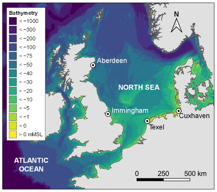
Figure 1 Study area and locations of the tide gauges. Bathymetry was provided by EMODnet Bathymetry Consortium (2020).

The British tide gauges in Aberdeen and Immingham have already been used in several previous studies (Gönnert, 2003), sometimes alongside additional tide gauges on the British coast (Koopmann, 1962). The height of the external surge at the Aberdeen tide gauge was used as a proxy for the height during its entrance into the North Sea (Bruss et al., 2011; Ganske et al., 2018), while Immingham is close to the location where most external surges reach their maximum height. The model of Bork and Müller-Navarra (2005) determines the maximum height to occur at the estuary The Wash, about 55 km south of the Humber Estuary, which coincides with the location of the maximum tidal range on the eastern British coast (ABPmer, 2008). However, the Immingham tide gauge provides more comprehensive data and shows only a small difference to tidal ranges in The Wash. Hence, these first two tide gauges can be assumed to be representative of important characteristics of external surges. The tide gauge in Cuxhaven has been regularly used as reference tide gauge in German coastal protection considerations, as it provides a continuous data series (a continuous record has been available since 1918 and tidal high and low waters since 1843) and is influenced neither by barriers like the East Frisian Islands nor by the Elbe Estuary fluxes. These three tide gauges have also been used in the study by Gönnert (2003), which serves as a benchmark for the present study. Additionally, the present study uses the tide gauge Texel Noordzee (hereafter called Texel) because it is located at an almost even distance to Immingham and Cuxhaven and can thus supplement information about the propagation of external surges after they reached their maximum height near Immingham. Water levels at these tide gauges are influenced by the local bathymetry, such as their position in an estuary or harbour basins, or man-made structures like breakwaters (Spencer et al., 2015; Serafin et al., 2019). Still, these tide gauges are used in the herein conducted study, as they cover the desired timespan, maintain comparability and quantify the effects of external surges on coastal areas, which is the main focus of this study. Inaccuracies in the height of the external surge due to variations of density (Mehra et al., 2009) and runoff in the estuary (Müller-Navarra and Bork, 2011) fall within the general uncertainties of the study, e.g. due to the calculation of astronomical tides.

2.2 Data acquisition and processing

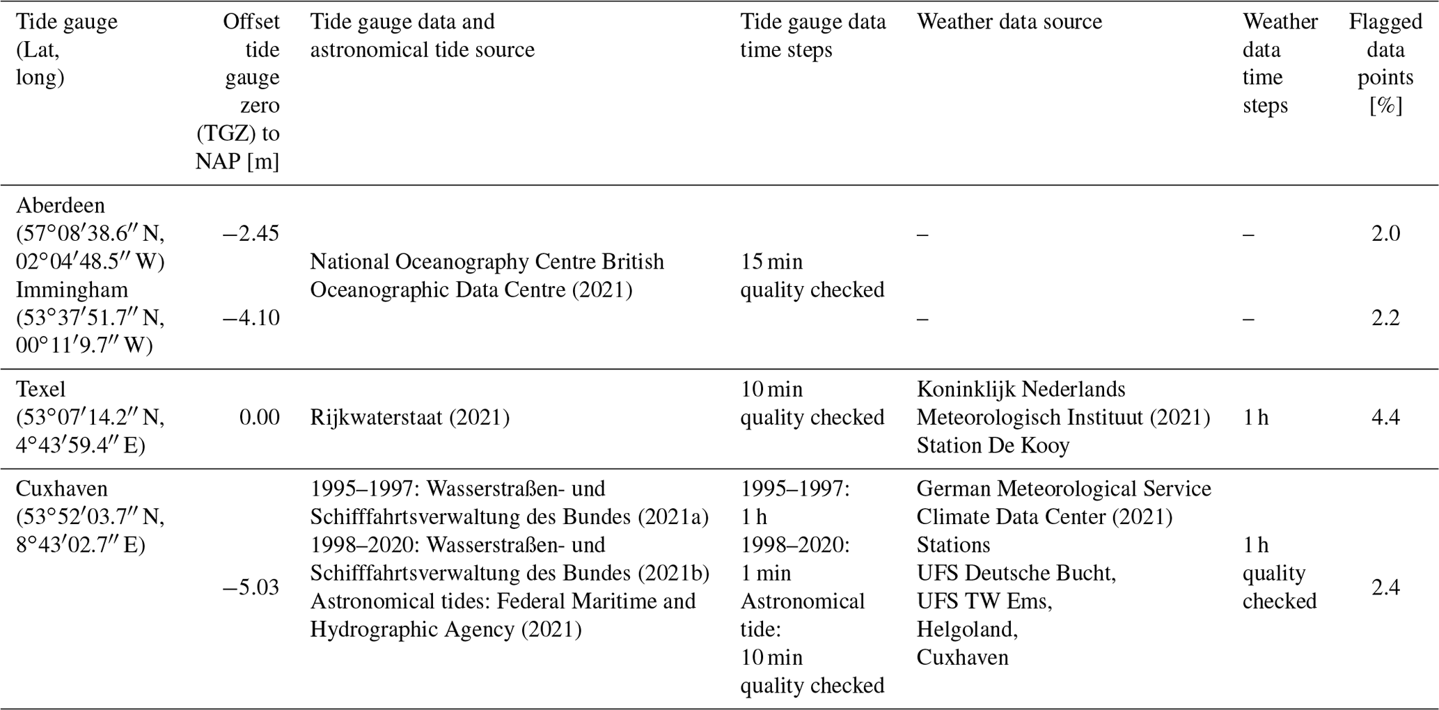
All data used in this study were provided by local authorities, mostly through open-access data portals. To receive uniform input data, all data were filtered to contain only hourly measurements, and tide gauge data as well as astronomical tides were transformed to be in reference to the Amsterdam Ordnance Datum (NAP). Missing or unlikely data like wind speed above 35 m s⁻¹ and air pressure above 1050 hPa or below 950 hPa were flagged and combined with the flags from the quality checks of the data providers. In the data of the tide gauge in Texel, two gaps, spanning more than a week, exist between 11 January and 22 November 2002 and 16 June and 2 July 2020. Flagged values are still used in the calculation of residuals, as the flags can also indicate successfully verified data. Overall, of the 227 928 data points per location, the fractions flagged as missing or unreasonable are given in Table 1.

Table 1 Location, offset to NAP, data sources and percentage of flagged data (flags from the data providers, as well as missing and unreasonable values) for each measurement station.

The weather data used to hindcast wind setup at the tide gauges in Texel and Cuxhaven are provided by the meteorological institutions as the following products:

• mean wind direction (average of the last 10 min before the full hour),

• mean wind speed (averaged accordingly) and

• air pressure reduced to sea level.

2.3 Methodological approach to identify external surges

To isolate external surges from hydrographic records, all other major components have to be eliminated. The methodology was developed by Gönnert (2003) but was adapted for this study to make the time steps independent from tidal cycles and therefore enable a more refined analysis. While Gönnert (2003) used the average residual between high and low water, resulting in time steps of 6.25 h, here the time steps are shortened to 1 h, allowing more precise assertions of the duration, height and timing of the events. Figure 2 gives an overview of the general steps in this process, consisting of three automated steps, each eliminating one contributor to water levels, and the consecutive manual quality check. Each step is explained in further detail in the following three subsections.

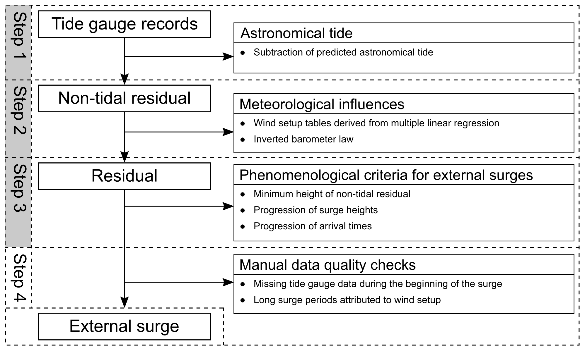
Figure 2 Schematic representation of the process to identify external surges. Grey backgrounds mark automated steps in the analysis.

2.3.1 Calculation of the non-tidal residual

First, the astronomical tide (h_astro) is eliminated from the water-level records to retrieve the non-tidal residual (Δh). The analysis and prediction have a long history on the North Sea coast and are still continuously improved (e.g. Amin, 1982; Müller-Navarra, 2013; Boesch and Müller-Navarra, 2019). As continuous predicted tides are available from the respective authorities, no separate analysis is conduced in this study. By removing the predicted tide, the non-tidal residual remains, which includes all parts of the water level, which do not follow the harmonic forcing of the sun and the moon:

$$\begin{array}{}\text{(1)}& \mathrm{\Delta }{h}_i=h_{\mathrm{obs},i}-h_{\mathrm{astro},i}.\end{array}$$

2.3.2 Wind setup hindcast

In step 2, the influence of meteorological factors on the non-tidal residual during external surges has to be discussed to derive the wind setup and the residual individually. In this study, wind setup describes the effect of wind and air pressure on the water level but only including local forcing. The residual therefore describes the remaining components of the water level, for example, remote meteorological forcing, lateral oscillations or the influence density variations. The methodology to determine the wind setup varies between the tide gauges due to different local and regional bathymetry and time lag between wind and water-level maxima (Proudman and Doodson, 1926; Dibbern and Müller-Navarra, 2009). For the British tide gauges, Rossiter (1959) developed empirical forecast formulae based on air pressure gradients from five sample points over the North Sea and northeast Atlantic, which can be attributed to wind directions and speeds. For the Aberdeen tide gauge, he concluded that residuals mainly depend on the following:

• local air pressure deviations, using the base value of 1012 hPa;

• northeast winds over the North Sea, with a time lag of 3 h;

• return surges that occur approximately 15 h after southerly winds over the northern North Sea;

• westerly winds over the North Atlantic, with a time lag of 9 h, causing or driving external surges.

Due to the different main wind direction, the coincidence of either two of the last three factors would require significant and sudden changes in wind conditions.

For the Immingham tide gauge, Rossiter (1959) concluded that the following parameters influence the residuals the most:

• the residual in Aberdeen with a time lag of 5 h and

• northeast winds over the North Sea with a time lag of 6 h.

The first accounts for local air pressure as well as external surges propagating southwards along the British coast. As the entrance of external surges is hindered by easterly winds, these two main factors are assumed to not coincide in general. For these two British tide gauges it can therefore be assumed that wind setup does not need to be accounted for during the detection of external surges, which was proven successfully in previous studies (Gönnert, 2003). Further research on the meteorological conditions causing external surges is certainly needed, especially focusing on wind and air pressure patterns. This detailed analysis could also enable more detailed statements about the co-occurrence of the weather patterns that cause non-tidal residuals in Aberdeen and Immingham. This analysis is, however, beyond the scope of this study but will be the focus of further work on external surges in the North Sea. The influence of other factors like water and air temperature or wind setup should be taken into consideration during the interpretation of surge heights, nonetheless.

For the tide gauge in Cuxhaven, Müller-Navarra and Giese (1999) developed an empirical forecast model using multiple linear regression (MLR) of various meteorological input factors like quadratic and cubic wind speeds of the zonal and meridional winds, air and water temperature gradients, static air pressure, and short-term air pressure changes as well as increases in water levels spanning multiple tide phases or stemming from the Atlantic. Wind setup tables, using wind speeds and directions as input, were provided by the Federal Maritime and Hydrographic Agency (BSH) and used to hindcast the expected wind setup. These tables group the measurements by two criteria to account for non-linear interactions between tide and wind setup:

• Tidal phase. Based on the height of the hindcast astronomical tide, the data points are split into high- (HW, h_astro>0 cm above NAP) and low-water phases (LW).

• General wind direction (onshore or offshore). Wind directions are split orthogonally to the main wind direction. The main wind direction, which produces the highest wind setup, was determined to be around 295^∘ in Cuxhaven (Annutsch, 1977; Gönnert, 2003). Winds between 20 and 200^∘ are offshore wind, resulting in negative wind setup in the German Bight.

The time lag between wind measurements and water-level deviation is given by Müller-Navarra and Giese (1999) with 3 h. For the influence of static air pressure, the inverted barometer law is used. It states that a decrease in air pressure by 1 hPa correlates linearly to an increase in water level by 1 cm (Koopmann, 1962), even though this correlation is simplified and can vary depending on local factors (Ponte and Gaspar, 1999; Müller-Navarra and Giese, 1999; Olbert and Hartnett, 2010). A simplified analysis of wind setup in Cuxhaven, using only wind and air pressure measurements, determined linear factors between 0.9 and 1.25 cm hPa⁻¹, depending on tidal phase and main wind direction, showing that the proposed value of 1 cm hPa⁻¹ is a good first approximation of the relationship. The other predictors of the forecast model are omitted due to lack of data (air and water temperatures) or because they anticipate the effect of external surges, as they can last several tidal phases and enter the North Sea from the Atlantic. This certainly reduces the accuracy of the hindcast and has to be discussed during analysis of the height of the external surges, but previous studies have produced satisfactory results based on wind and air pressure data (Dibbern and Müller-Navarra, 2009; Jensen et al., 2013). At the Texel tide gauge, a simplified method of this forecast model, which was introduced by Dibbern and Müller-Navarra (2009), is used to calculate wind setup tables and the air pressure coefficient. The method defines the water level as the weighted sum of multiple terms depending on meteorological measurements. The functions and units of the six terms are given in Table 2.

Table 2 Functions to produce MLR input.

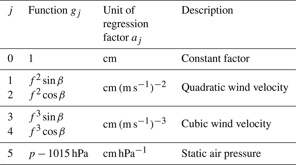
Function 0 is a constant term for the difference between the neutral sea state and RMSL. Functions 1 and 2 are the orthogonal components of the quadratic wind stress; functions 3 and 4 add the cubic wind stress. Function 5 accounts for static air pressure and uses the same assumption as the IBL. The weighted sum of these terms gives a prediction of the measured non-tidal residual. In Eq. (2), deviations from the measured height are incorporated by an error term:

$$\begin{array}{}\text{(2)}& \mathrm{\Delta }{h}_{\mathrm{obs},i}=\sum _{j=\mathrm{0}}^J{a}_j{g}_j\left({\mathit{x}}_i\right)+e_i=\mathrm{\Delta }{h}_{\mathrm{pre},i}+e_i.\end{array}$$

An MLR optimizes the regression factors for the least square error. The total of the squared errors is defined in Eq. (3), which is taken from the detailed description of the procedure in Müller-Navarra and Giese (1999).

$$\begin{array}{}\text{(3)}& {\mathit{\chi }}^{\mathrm{2}}\left(\mathit{a}\right)=\sum _{i=\mathrm{1}}^I{e}_i^{\mathrm{2}}=\sum _{i=\mathrm{1}}^I\left(\mathrm{\Delta }{h}_i-\sum _{j=\mathrm{0}}^J{\left(a_j{g}_j\left({\mathit{x}}_i\right)\right)}^{\mathrm{2}}\right)=\min \end{array}$$

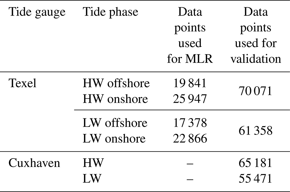
Data are again grouped into four by tidal phase and wind direction. The MLR is conducted for each group individually. Data from 1995 to 2004 are used to determine the regression factors so that independent validation of the regression results can be conducted using the 2005 to 2020 data. The 2005 to 2020 data are also used for the Cuxhaven tide gauge to verify the wind setup tables of the BSH. Table 3 gives the number of data points used in each regression and validation. Flagged data points are not included in the regression data, as the flags do not accurately distinguish between verified or corrected and flawed data. Data points with wind speeds above 20 m s⁻¹ are not included as well because these rather rare events show great variability and have a strong influence on the regression factors, causing an overall worse hindcast if included.

Table 3 Overview of the remaining data points available for MLR and validation for Texel and Cuxhaven subdivided into tide-phase groups.

The accuracy of the hindcast can be assessed by calculating the root mean square error (RMSE) of the verification period (2005–2020):

$$\begin{array}{}\text{(4)}& e_{\mathrm{RMS}}=\sqrt{{\displaystyle \frac{\sum _{i=\mathrm{1}}^I{\left(\mathrm{\Delta }{h}_{\mathrm{obs},i}-\mathrm{\Delta }{h}_{\mathrm{pre},i}\right)}^{\mathrm{2}}}{I}}}.\end{array}$$

For the tide gauge in Cuxhaven, the RMSE is used to verify the time lag of 3 h between wind measurements and predicted water levels, which was determined by Müller-Navarra and Giese (1999). The hindcast model generally performs better for high-water phases, with a minimum RMSE of 18.5 cm compared to 20.8 cm for low water. Both minima are determined with a time lag of 4 h, but the strong increase in a time lag of 5 h suggests an optimal time lag between 3 and 4 h, corresponding generally with the assumption of Müller-Navarra and Giese (1999). The relation between the RMSE and the time lag is shown in Fig. 3.

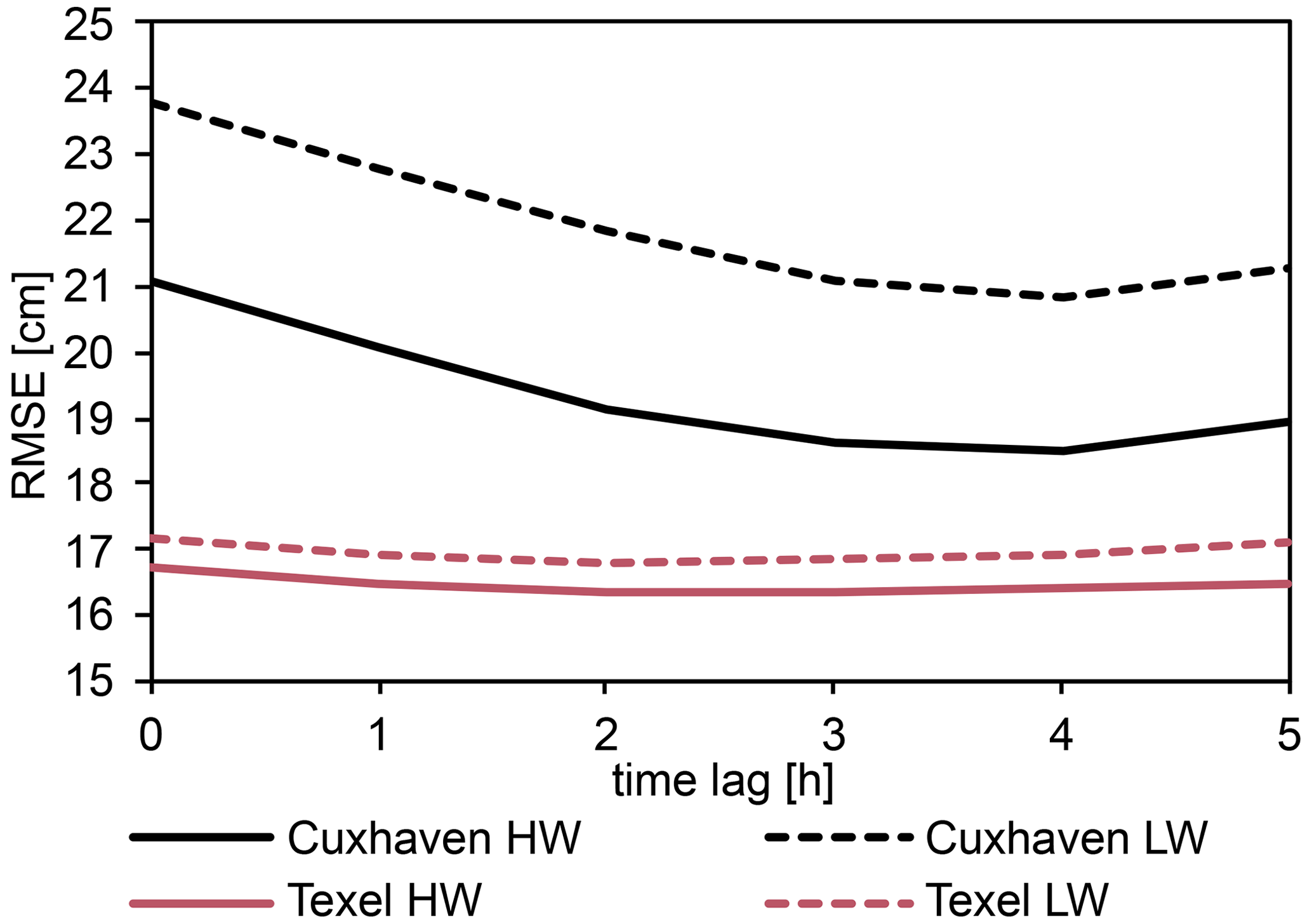
Figure 3 RMSE depending on the time lag between measured winds and wind setups at the tide gauges in Cuxhaven (black lines) and Texel (red lines). Solid lines mark the RMSE for high-water phases and dashed lines for low-water phases. The groups, based on off- and onshore wind directions, are combined before determining the RMSE.

For the Texel tide gauge, the unknown factors of main wind direction and time lag between wind and water level have to be determined as well. First, the RMSE is calculated for multiple MLRs with varying main wind directions and the separation between onshore and offshore wind at ±90^∘ of the main direction. The optimal limit between on- and offshore wind is found to be around 20 and 200^∘, which is close to the general orientation of Texel's coast. The optimization of the time lag is shown in Fig. 3, which determines a time lag of 2 h. The RMSE is lower than in Cuxhaven with 16.3 cm for high-water and 16.8 cm for low-water phases.

Table 4 Regression factor a_i for the tide gauge in Texel and statistical significance of each component. Statistical significance is determined at the 95 % confidence level.

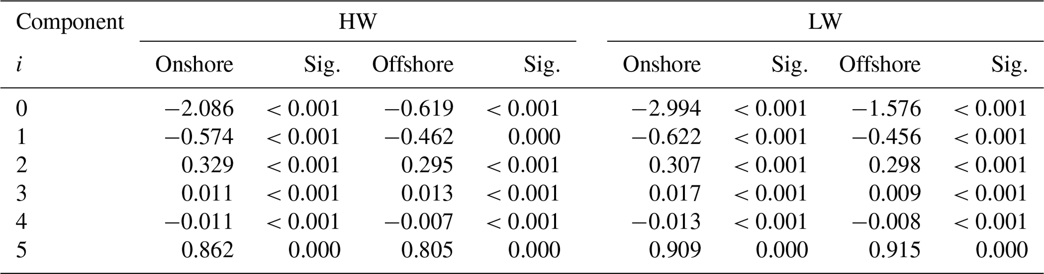
Table 4 lists the regression factors for the optimal main wind direction, the time lag for the tide gauge in Texel and their statistical significance at the 95 % confidence level for the four groups of data points. The air pressure coefficient for example varies between 0.805 and 0.915, meaning that the dependence on static air pressure is more uniform than in Cuxhaven but slightly smaller than predicted by the IBL.

In Eq. (5), the regression factors of components 0 to 4 are used to compile wind setup tables similar to those of the BSH:

$$\begin{array}{}\text{(5)}& \begin{array}{rl}\mathrm{\Delta }{h}_{\mathrm{W},i}& =a_{\mathrm{0}}+\left(a_{\mathrm{1}}\sin {\mathit{\beta }}_i+a_{\mathrm{2}}\cos {\mathit{\beta }}_i\right)f_i^{\mathrm{2}}\\ & +\left(a_{\mathrm{3}}\sin {\mathit{\beta }}_i+a_{\mathrm{4}}\cos {\mathit{\beta }}_i\right)f_i^{\mathrm{3}}.\end{array}\end{array}$$

The tables contain the calculated wind setup in steps of 1 m s⁻¹ and 5^∘. To mitigate the effects of spikes or troughs and to further account for the delayed reaction of wind setup, the wind setups are averaged over 3 h from 2 h before the timestamp to 1 h after the timestamp. For Cuxhaven, the wind setup is calculated from the winds from 5 to 2 h before the water-level measurement.

Additionally, the water-level deviation due to air pressure is calculated in Eq. (6):

$$\begin{array}{}\text{(6)}& \mathrm{\Delta }{h}_{\mathrm{AP}}=a_{\mathrm{5}}(p-\mathrm{1015}\mathrm{hPa}).\end{array}$$

For Cuxhaven, where the IBL is used, a₅ equals 1 cm hPa⁻¹. To assess the quality of the hindcast, the calculated wind setup including the effect of static air pressure is plotted against the measured wind setup for both tide gauges and grouped by tidal phases in Fig. 4, using the verification time period.

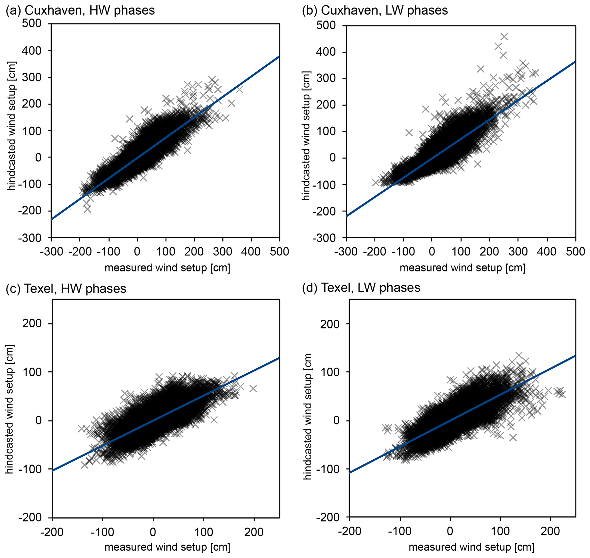
Figure 4 Comparison of hindcasts and measurements of wind setups in Cuxhaven (a, b) and Texel (c, d).

Hindcast and measurement are in good agreement, but they show a tendency to underestimate wind setup, which is more pronounced at the Texel tide gauge, with the exception of three hindcasts of high wind setup during low-water phases at the Cuxhaven tide gauge. This is probably due to the reduced set of predictors of wind setup. The method was tested for the British tide gauges as well but did not produce sufficient results, probably due to the wrong set of key predictors. Approaches to improve the wind setup for all locations are discussed in Sect. 4.

2.3.3 Calculation of the residual

The meteorological influences from wind setup and air pressure are used in Eq. (7) to calculate the residual in Cuxhaven and Texel. For the wind setup, the tables, which were compiled in Sect. 2.3.2, are interpolated linearly.

$$\begin{array}{}\text{(7)}& \mathrm{\Delta }{h}_{\mathrm{R}}=\mathrm{\Delta }h-\mathrm{\Delta }{h}_{\mathrm{W}}-\mathrm{\Delta }{h}_{\mathrm{AP}}\end{array}$$

During timespans where only tides and local meteorological forcing influence the water level, the residual should be approximately 0 cm, but many deviations remain, which may be caused by external surges, but can also be due to the simplified approach to hindcast the wind setup, natural variability or other local phenomena. To find a collective term for these deviations, we call them surges, without specifying their origin. In step 3, the surges are filtered for external surges based on the following conditions proposed by Gönnert (2003):

• The non-tidal residual in Aberdeen is greater than 40 cm.

• Surge heights generally increase from Aberdeen to Immingham, caused by local winds, with a maximum decrease of 10 cm.

• The arrival in Immingham is at least 2 h later than in Aberdeen but no more than 5 h later. The time of arrival is defined as the time when the non-tidal residual is over 10 cm in height.

For each external surge, the maximum height and arrival time at each tide gauge are determined and the non-tidal residual (for Aberdeen and Immingham) or the residual (for Texel and Cuxhaven) as well as the data quality flags are plotted from 6 h before the arrival of the external surge in Aberdeen to 42 h after the arrival.

Finally, a manual quality check is conducted on the plots of the external surges. A total of four surges were eliminated due to either of the following reasons:

• missing tide gauge data during the beginning of the surge in Aberdeen or Immingham (the height or the offset of the surge may be influenced by these missing values) and

• long surge periods that can be attributed to wind setup in Aberdeen and Immingham.

2.4 Sensitivity analysis

Criteria for external surges are assessed by varying the minimum height in Aberdeen and the maximum offset between Aberdeen an Immingham. The minimum height in Aberdeen is found to be suitable for the uncertainties of the hindcast of tides and wind setup. If the minimum height is reduced by 10 cm, more than 50 % of the additionally detected surges cannot clearly be differentiated from fluctuations in residuals due to wind setup and other factors. For an increase of the temporal offset from 5 to 7 h, the error rate is only 24 %, meaning that 76 % of the additionally detected surges match external surges in their general behaviour like heights at the four tide gauges and periods. However, to maintain comparability between this study and the study conducted by Gönnert (2003), these surges are not included in the dataset. Moreover, external surges have to be studied further to discern whether an offset of 7 h between Aberdeen and Immingham is physically possible. This would require extensive research about the propagation of external surges, which is beyond the scope of this paper. Using the dataset with a longer allowed offset between Aberdeen and Immingham would, however, invalidate the comparison of data collected by Gönnert (2003) and this study.

2.5 Meteorology

External surges found in this study are mainly compared to the dataset of Gönnert (2003), which spans the years 1971 to 1995. To distinguish between the datasets, the dataset of Gönnert is hereafter called DataSet1, and the dataset derived from the automated approach is called DataSet2.

The occurrence of external surges in the North Sea basin is strongly coupled to storm systems in the North Atlantic. Although the process of the physical meteo-oceanic coupling is not within the scope of this work, it will be important to correlate the observations from the tide gauge data to general weather patterns. To briefly repeat meteorological conditions in a context of surge generation, the European weather situations during the beginning of the observed external surges are assembled first. The European weather situations were originally defined by Hess and Brezowski (1977) and determined by Werner and Gerstengarbe (2010) for the duration from 1881 to 2009. From 2010 onwards, the records from the German Meteorological Service (2021) are used. The Agency for Roads, Bridges and Waters Hamburg (2012) found 61 of the 73 external surges of DataSet1 to occur during four weather situations (western situation cyclonic: WZ, western situation anticyclonic: WA, southwestern situation anticyclonic: SWA, high-pressure bridge central Europe: BM).

The characterization of external surges with respect to low-pressure cells can be summarized from Werner and Gerstengarbe (2010) as follows:

• WZ. Single disturbances with high-pressure cells in between travel from Ireland over the British Isles and North and Baltic Sea towards eastern Europe. The driving low-pressure cells are located north of 60^∘ N.

• WA. The central low-pressure cell is often located north of 65^∘ N with single disturbances travelling from the west of Scotland over Scandinavia towards the Baltic.

• SWA. A low-pressure system is mostly located over the middle of the North Atlantic and the western Norwegian Sea. Single disturbances travel to the northeast.

• BM. A high-pressure bridge is located between the Azores and eastern Europe with an eastward-directed frontal zone north of it and single disturbances travelling eastwards.

In the analysis of DataSet2, an additional weather situation is identified that correlates with an increased number of external surges (NWZ, northwestern situation cyclonic) and has the following characteristics:

• NWZ. It is characterized by having an extensive low-pressure area over Scotland, the Norwegian Sea and Scandinavia with single disturbances travelling over the British Isles towards eastern central Europe.

A detailed analysis of weather situations is presented in Sect. 3.2, while Sect. 3.3 analyses the influence of external surges on storm surges in the German Bight.

3 Results

3.1 The phenomenon of serial external surges

Overall, 65 external surge events were identified between 1995 and 2020 (labelled DataSet2); the statistical base parameters of this new dataset are listed in Table 5.

Table 5 Total number of external surge events and external surges in the datasets.

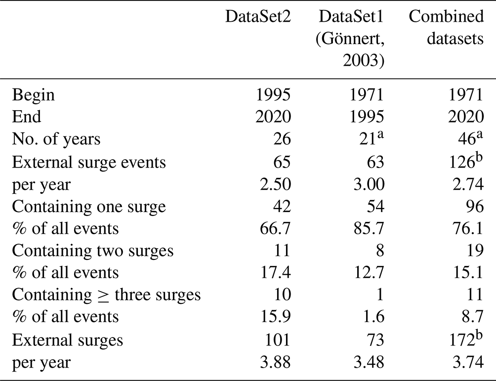
^a In total 4 years with missing data (1974–1977) are deducted; ^b two events that are part of both datasets (18 January and 1 February 1995) are deducted.

Several of those events consist of more than a single external surge and are identified as a sequence or series of external waves in the residual water-level oscillations. Figure 5 gives examples of both a single external surge (Fig. 5a) and an event consisting of three external surges (Fig. 5b), arriving with gaps of 22 h between the first and second surge and 43 h between the second and third surge. For those events, it is possible that they depend on the same meteorological origin caused by storm systems in the northeast Atlantic. Moreover, they can interact with each other in the North Sea, as they can remain there for more than 48 h depending on their celerity and wavelength. This can also be seen in Fig. 5b: during the arrival of the second external surge in Aberdeen, the residual at the Cuxhaven tide gauge is still at around 30 cm caused by the first external surge. It also shows possible effects of the interaction of the first two surges: while the two external surges are mostly uniform and of similar height in Aberdeen and Immingham (the peak height varies by around 15 cm), the second external surge is 30 cm higher in Texel and 50 cm higher in Cuxhaven. To verify whether this behaviour is caused by interactions of the two external surges or other influences, more detailed studies should be conducted using numerical models or residuals at other tide gauges. In this study, the term “serial external surges” is used for series of identified external surges in close succession. In total, 101 external surges were found in 65 external surge events. Some of those external surges were also detected by the automated detection but grouped with other external surges; others do not match the required height or offset between Aberdeen and Immingham but were identified during the manual review of the external surges. Since they occurred shortly before or after a detected external surge, and preceding external surges may alter the height and timing of the external surge, they are also included in the dataset. The grouping into external surge events has therefore been conducted manually.

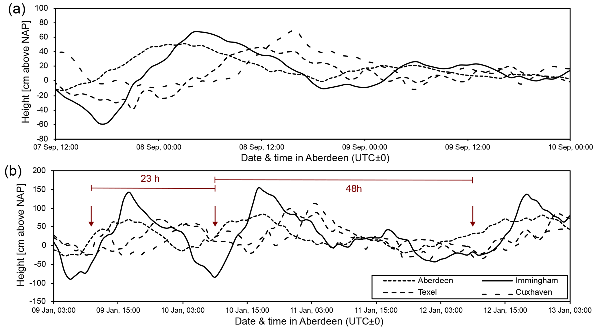
Figure 5 Height of the non-tidal residual (at the gauges in Aberdeen and Immingham) and the residual (in Texel and Cuxhaven) for examples of an external surge on 7 and 8 September 2000 (a) and a serial external surge on 9–13 January 2015 (b). The arrows in (b) mark the beginning of the external surges in Aberdeen (residual > 20 cm), and the timing between the serial external surges is given.

Figure 6 shows the heights of each external surge and the time since the previous external surge (note the logarithmic scale). Additionally, the sum line of events depending on their time since the previous surge is also shown.

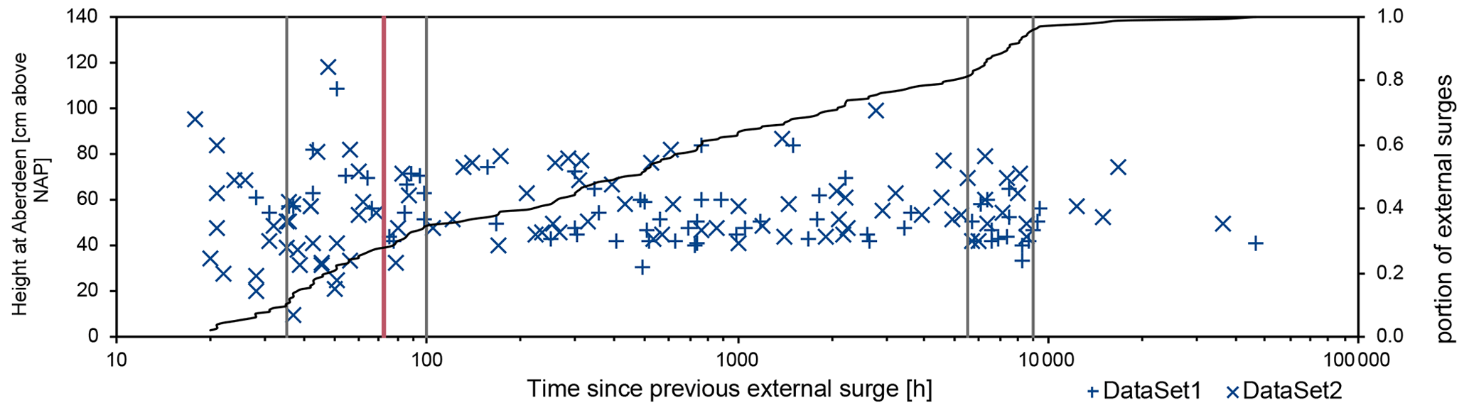
Figure 6 Height of the external surges (combined datasets) over the time since the previous surge and the sum line of external surges depending on the time since the previous surge. Two areas of stronger increases can be seen (highlighted by the grey lines): between 35 and 100 h and between 5500 and 9000 h. The first shows the occurrence of serial external surges, and the second is due to the lack of external surges in spring and summer, resulting in similar gaps between the last surge in winter and the first surge in autumn. The red line shows the threshold of 72 h for serial external surges.

A closer inspection of the sum line reveals two frequency peaks: one peak exists for external surges occurring less than 100 h after the last surge, and the second peak is for a timespan between 230 and 375 d (5500 and 9000 h). The second peak originates from the very rare occurrence of external surges during spring and summer months, resulting in similar timespans between the last surge in winter and the first surge in the following autumn. The first peak however indicates that the frequency of serial external surges is way higher than would be expected by the random close occurrence of two independent external surges. A threshold duration of 72 h is chosen, as the definition of serial external surges should not only include their increased occurrence, but also their origin (the same or closely succeeding low-pressure cells) and their possible impact (interaction with each other and modulation of storm surges). The occurrence of serial external surges has not been addressed in the recent literature so far.

In DataSet2, a third of the external surge events consisted of more than one surge. Of those, 11 events contain two surges, and the other 10 contain three or more surges. One special event can be found in February 1997: from 18 February onwards, six consecutive external surges were detected, all within 72 h of each other. The calculated residuals for this event are plotted in Fig. 7.

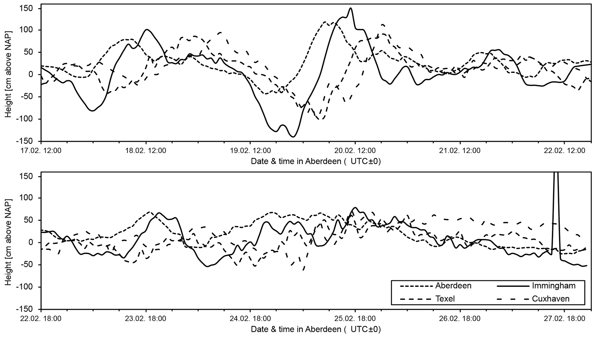
Figure 7 Height of the non-tidal residual (at the gauges in Aberdeen and Immingham) and the residual (in Texel and Cuxhaven) during the serial external surges from 17 to 27 February 1997. The fourth surge, starting on 22 February at 06:00 LT in Aberdeen, does not reach the required height limit. However, if the preceding troughs are considered, this surge reaches 39 cm in Aberdeen and 48 cm in Immingham and can therefore be considered an external surge. The spike in Immingham around 27 February 15:00 LT is due to uncorrected flawed data.

This series of surges lasted until 27 February. From 28 February to 3 March two additional surges can be seen in the residuals that loosely resemble external surges but do not match the criteria defined previously. The weather conditions in northwestern Europe were consistent during the period with westerly winds and low-pressure cells over the Atlantic, which match the conditions that Gönnert (2003) found to be the most prominent during the detection of external surges.

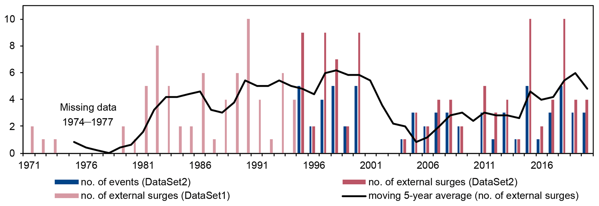
Figure 8 Number of external surges per year and moving 5-year average, both from this study and Gönnert (2003). The 5-year average is accurate from 1983 onwards, as previous values include years with missing data. From 1995 onwards, the number of events is also shown, which counts serial external surges as a single event.

The dataset from Gönnert (2003) (labelled DataSet1) was not previously analysed with regards to serial external surges. This study hence uses that dataset with a focus on detecting additional serial surge events, appending them to those found in the 1995 to 2020 dataset. In total 73 external surges can be grouped into 63 events. In eight cases or 12.7 % of the external surge events, two external surges were detected less than 3 d apart, which is slightly less than in DataSet2. By contrast, only one event containing three surges is found so that the overall percentage of serial external surges is lower in this dataset. This aberration might be due to the different time steps of the analysis and cannot be interpreted as a significant trend. All in all, 30 serial surge events are identified; of those, 19 consist of two surges and 3 of four or more (see Table 5).

3.2 Frequency and height of external surges in the North Sea

Figure 8 shows the number of external surges per year for both datasets and their moving 5-year average.

In comparison to the external surges found by Gönnert (2003), the total number of external surges increases, while the number of external surge events decreases slightly. The increased number of external surges can mainly be explained by the higher temporal resolution that enables a clearer distinction between single external surges and the focus on serial external surges. On the other hand, the decrease in the number of external surge events is rather small and can mainly be attributed to the period from 2001 to 2006, when only six events were detected. Due to this variability in their occurrence, no significant trend can be determined, as linear, polynomial or logarithmic trend lines predict an increasing, constant or falling number of external surges respectively.

The distribution of external surges over the year (see Fig. 9) – an important distribution with respect to its co-influence with wind surge effects in coastal waters – is not equal but shows a strongly increased occurrence during autumn and winter months with January having the highest number of external surges.

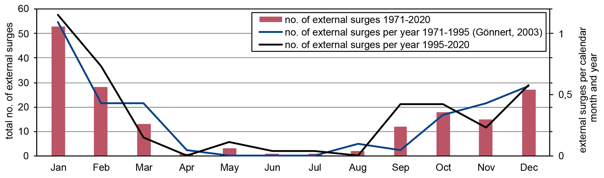
Figure 9 Number of external surges per calendar month; the data from Gönnert (2003) contain a data gap from 1974 to 1977, which does not influence the monthly distribution, as whole years are missing.

Only eight of the 172 external surges from DataSet1 and DataSet2 occurred during the spring and summer months from April to August. The comparison of distributions between the two datasets shows a 10-fold increase in external surges in September and a decrease of 65 % in March. This may hint towards a shift of the main external surge season to start earlier in the year but also end earlier. As of now, the datasets do not span a sufficient timeframe to verify this assumption. A one-tailed t test (using the day of arrival after 1 July) found earlier arrival by 6 d between DataSet1 (M=183.0, SD = 50.5) and DataSet2 (M=177.1, SD = 63.3). However this difference was not found to be significant (t(170)=0.681, $p=\mathrm{0.248}>\mathrm{0.05}$).

The height of the external surges matches previous studies and simulations (Schmitz et al., 1988; Gönnert, 2003; Bork and Müller-Navarra, 2005). Figure 10 shows boxplots of the heights of the recorded external surges.

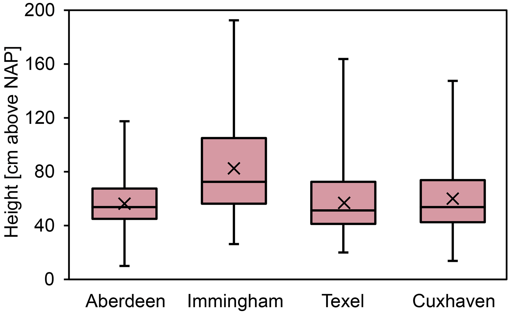
Figure 10 Boxplot of the heights of external surges in Aberdeen, Immingham, Texel and Cuxhaven from 1995 to 2020. Crosses mark the mean, and the boxes represent the upper and lower quartile with the horizontal line for the median. The whiskers show the minimum and maximum height.

Beginning with an average height of 56 cm in Aberdeen, the external surge height increases along the British coast and reaches 83 cm in Immingham. During their propagation along the southern and southeastern coast of the North Sea, their averaged height decreases to 57 and 60 cm at the Texel and Cuxhaven gauges respectively. Nonetheless, the maximum height of the external surges can reach 100 cm in Aberdeen with a single even higher event with 118 cm. The highest overall surge height was recorded in Immingham with 192 cm. In Texel and Cuxhaven, the highest events are also more than double the average height with 164 and 148 cm respectively. The most extreme event in Texel should be further assessed, as it is almost 60 cm higher than the second highest. This exceptionally high external surge was recorded on 5 December 2013 as the storm Xaver also crossed the North Sea. The predictability of heights based on the British tide gauges is higher in Texel than in Cuxhaven. For both locations, the height is more closely related to the height in Immingham than in Aberdeen. The ratios of heights $\frac{h_{\mathrm{Tex}}}{h_{\mathrm{Imm}}}$ and $\frac{h_{\mathrm{Cux}}}{h_{\mathrm{Imm}}}$ show 3 times the variance in Cuxhaven compared to Texel. In Texel, only seven of the 101 external surges are recorded higher than in Immingham with a maximum increase of 17 cm. These growing surges reach heights between 58 and 103 cm in Texel. An increase in heights between Immingham and Cuxhaven is also rare but more prevalent with 20 % of the events showing a height increase. Among those are two of the highest recorded surges, reaching 148 and 121 cm. The closer correlation between Immingham and Texel can be explained by the shorter distance and minimizing potential for currents or local weather to influence the surge height.

3.3 Classification based on meteorological conditions

Figure 11 correlates the weather situations as per Hess and Brezowski's (1977) definition (see Sect. 2.5 for the description of the weather patterns) with the number of external surges that was detected at the time of the weather situation.

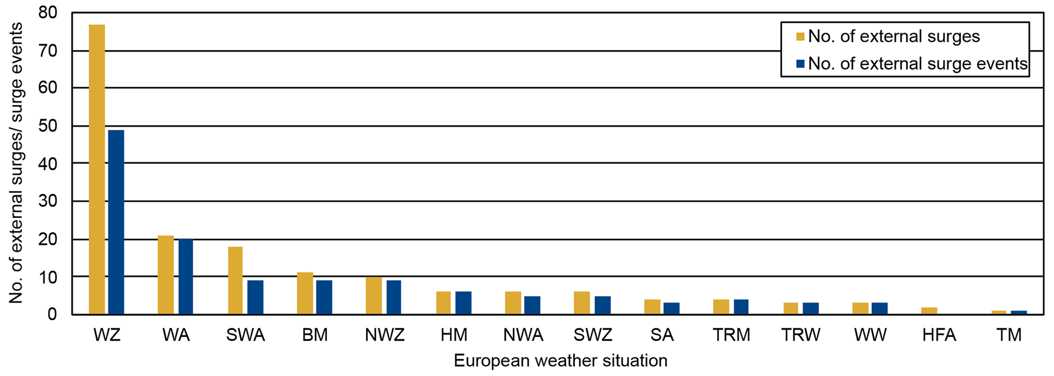
Figure 11 Number of external surges per European weather situation of the 1971 to 2020 external surges. Weather situations are defined by Hess and Brezowski (1977). The weather situation of an external surge is the one that is present at the date of arrival in Aberdeen. For an external surge event, the weather situation of the first or only surge in the series is used. For the weather situation HFA, no external surge event is noted, as both external surges occurred as part of a series that started during a different weather situation.

The Agency for Roads, Bridges and Waters Hamburg (2012) already collected the weather situations during the years 1971 to 1995 and found that the weather situation WZ produces by far the most external surges with about half of the external surges being recorded during this weather situation. The three other main weather situations that were found during external surges are WA, SWA and BM. These weather situations show the characteristics that were previously associated with external surges in the North Sea with low-pressure cells over the North Atlantic and disturbances travelling eastwards and account for more than 80 % of the detected external surges. Including DataSet2, an additional main weather situation prone to generating external surges (NWZ) is however identified. From only three external surges in the older dataset, the number of external surges during this weather situation more than doubles. Two other weather situations also show an increase in relevance: BM and SWA. Meanwhile, the share of external surges caused during the weather situations WZ and WA slightly lost relevance. Still, these variations lie within the natural variability of the occurrence of external surges.

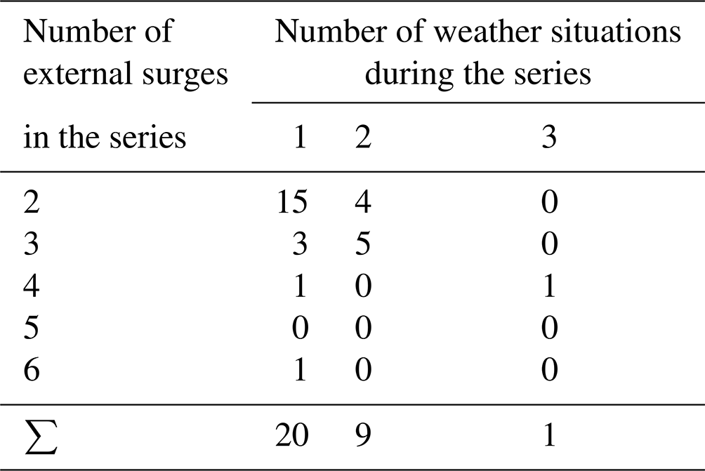
Serial external surges seem to be more prevalent during certain weather conditions, namely WZ and SWA situations, which show the highest ratios of external surges to the number of external surge events. They also seem to be supported by long-lasting weather situations. Table 6 shows that 20 of the 30 serial events did not happen during changing weather situations, including the series of six external surges, and only one event (consisting of four external surges) was driven by three different weather situations.

Table 6 Number of serial external surges depending on the number of external surges in the series and the number of weather situations during the start of the contained external surges.

These observations are based on a rather small sample size, so they should be assessed by further, more detailed studies of the weather conditions that cause external surges, for example, the analysis of travel paths of the low-pressure cells. The weather situation also influences the average height of the external surges with the highest occurring during WZ and BM conditions with 57 cm in Aberdeen and the lowest during the SWA situation only reaching 51 cm.

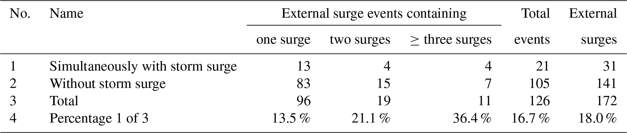
Table 7 Number of external surges and external surge events during storm surges.

3.4 Combined events of external surge and storm surge events

Increased water levels caused by external surges along the North Sea coast are of particular interest when it comes to co-occurrence with storm surge events. Storm surge events, in most cases, are composed of tide and wind surge. Combined events of tide, wind surge and external surges have the potential to cause extreme water levels along the North Sea coast, challenging current and future coastal protection strategies and actions. Therefore, analysing combined events of external and storm surges is an essential step. Combined events of external surge and storm surge events can be generated by two different meteorological situations: on the one hand, both phenomena are initiated by two different extra-tropical cyclones in close succession. Due to different propagation velocities both phenomena arrive at a tide gauge at the same time. On the other hand, both phenomena are initiated by the same extra-tropical cyclone (Gönnert and Gerkensmeier, 2015). Whether the wind setup is defined as a storm surge or not depends on the chosen definition of these events. For this analysis, storm surges are defined as events reaching peaks of at least +1.5 m above mean high water (moving average of the previous 5 years) in Cuxhaven, or a wind setup of at least 2 m is reached independently of the tidal phase (definition follows the determination of the Agency for Roads, Bridges and Waters Hamburg (2012), who is responsible for assessing the design water level for public coastal protection facilities of the Free and Hanseatic City of Hamburg). Following this definition, 21 % or 16.7 % out of 126 external surge events recorded between 1971 and 2020 occurred during or close to a storm surge event in the German Bight. Moreover, serial external surge events, a phenomenon that was analysed in this study for the first time, can be observed more frequently during combined events. Particularly the number of external surges in the series increases during combined events, compared to observed single events (see Table 7). As stated before, the statistical correlations have to be verified by further research about the interactions between external and storm surges.

With regard to a more detailed analysis of the average height of the external surges during storm surge events, DataSet2 shows an increase to an average of 64 cm in Aberdeen and 70 cm in Cuxhaven (compared to average heights without storm surges of 56 cm in Aberdeen and 60 cm in Cuxhaven as described in Sect. 3.1). It confirms former findings for average heights of external surges during storm surge events compiled for DataSet1 (1971–1995) (Agency for Roads, Bridges and Waters Hamburg, 2012). Local effects of the extra-tropical cyclones involved during the development of these combined events might play a role in this development. One special example of an external surge occurring during a storm surge is the external surge during the storm Xaver on 5 and 6 December 2013. The external surge, which was earlier detected by Fenoglio-Marc et al. (2015) using satellite altimetry, contributed to record water levels at some parts of the German coast (Dangendorf et al., 2016) and, in the present study, reached a calculated height of 146 cm at the Cuxhaven tide gauge. Upon closer inspection, this calculation was most likely influenced by missing wind records at some German weather stations, bringing the maximum height to 95 cm. Still, extraordinary heights were calculated in Immingham and Texel (Spencer et al., 2015; Kettle, 2020), highlighting the need for further, detailed analysis of single external events using multiple approaches to assess the occurrence and impact of the highest external surges.

4 Discussion

The automated detection of external surges presented in this study improves the possibility of faster and more detailed analysis of external surges, while past work had predominantly relied on manual interpretation of tide records. Using the automated algorithm (see Sect. 2.3), further tide gauges can be easily added to get a more detailed picture of heights, timing and velocity of external surges, and analysis might be expanded to the Danish or Norwegian coast. Moreover, for the first time, active application of the automated algorithm facilitates a continuous monitoring of external surge events. A reanalysis of the 1971 to 1995 period might also be possible and meaningful to find deviations due to the changes in the detection, but data assimilation and pre-processing is more time-consuming due to the increased temporal resolution. As of now, the automated detection cannot accurately detect all external surges in a series of external surges and differentiate between each external surge.

Additional characteristics of the external surges can also be analysed in future studies using the new dataset. For example, the meteorological conditions used in this study only resemble generalized classification. Analysis of the tracks of the low-pressure cells is important to understand their influence on the generation, propagation and surge characteristics. Combination with the analysis of storm tracks (e.g. Ganske et al., 2018; Horsburgh et al., 2021) is important to identify possible extreme events consisting of external surges and storm surges. Moreover, the enhanced dataset can be used to evaluate the time of arrival of external surges at certain tide gauges in relation to tides and the maximum wind setup to further investigate non-linear interactions.

By providing an adapted methodological approach, application of the study exposed further points for improvements with regard to detailed analysis of the characteristics of external surge events. This study showed a significant number of events similar to external surges with an offset larger than 6 h between Aberdeen and Immingham that are not yet considered in the dataset. Those events still need to be verified as external surges, for example, by numerical models and assessment of weather conditions. With regard to the measured height of external surges, which is strongly related to the height of the wind setup, this study used a simplified version of the hindcast method by Müller-Navarra and Giese (1999). A more complex approach, such as hindcast modelling of all relevant storm conditions, might improve the accuracy of the overall analysis. For this improvement, the predictors of Müller-Navarra and Giese (1999) have to be split into those that are independent of external surges and those influenced by them. Predictors like the residual in Aberdeen and residual spanning multiple tide phases can be included to separate local and far-field meteorological effects. They should, however, only be included during the determination of the regression factors, not in the calculation of wind setup. This way the effect of external surges on the regression is minimized, but external surges remain part of the residual. On the other hand, to better predict values between tide peaks and to quantify non-linear interactions, the height of the tide could be added as an additional predictor. Moreover, further improvement to increase the level of specification of the external surge heights could be reached by improving the hindcast method suitable for the British tide gauges. Using a modified set of predictors and suitable location for the wind data should produce results similar to those of Rossiter (1959), as he also used MLR to determine the optimal weights in his forecast. An accurate hindcast of wind setup at these locations could on the one hand improve the accuracy of the measured height and on the other hand enable a smaller height threshold for the detection of external surges, resulting in a more detailed dataset for future analysis.

The combination of the manually compiled DataSet1 from 1971 to 1995 and the new DataSet2 spanning the 1995 to 2020 period provides further insight into the occurrence of external surges in the North Sea and their variability in a decadal perspective. Findings resulting from the improved dataset can also be used to assess existing procedures on how to deal with extreme water levels and therewith have a direct effect on coastal protection in practice. In the particular case of the Free and Hanseatic City of Hamburg, the responsible authority, the LSBG is one of the few who explicitly considers external surges as an essential component of extreme-water-level events in their assessment (Gönnert and Müller, 2014). The design-level height is determined by a multi-method approach that analyses and includes non-linear interactions of all storm surge components (spring tide, wind surge and external surge). These non-linear interactions with spring tides and wind setup reduce the effective height of an external surge (Gönnert et al., 2010). The resulting design-level height in Hamburg incorporates an external surge with a height of 77 cm that results from the highest observed external surge reached at the tidal gauge in Aberdeen (1.08 m) and a determined reduction of 30 % on its way to Cuxhaven, due to non-linear interactions with a very high wind surge during an extreme storm surge event (Gönnert et al., 2010; Agency for Roads, Bridges and Waters Hamburg, 2012). The extended dataset provided the opportunity for the LSBG to verify the assumptions about external surges in its design-level concept for an even longer period. Thus, possible, necessary adjustments to the assumption about a maximum height of external surges in the context of an extreme storm surge event described above had to be examined and confirmed. Additionally, the design process of coastal defence structures considers local wave climate by limiting wave run-up and overtopping. Limiting the overtopping rate results in additional elevation (Pullen et al., 2007), which has to be added to the design water level, consisting of spring tide, wind setup and external surge. A local wave climate is, however, determined by the angle of attack and the significant wave height, which are, in contrast to the still water level, statistical properties. Methods to analyse wave climate therefore differ from those to analyse water levels (e.g. in Weisse et al., 2012); hence wave climate is not further considered in this study. It is, nonetheless, monitored alongside sea-level rise and storm surges to detect possible changes and plan the necessary adaption.

Resulting from this monitoring, serial external surges should be analysed as interdependent waves in the future, since they can influence peak water level in a couple of different ways depending on the timing between high waters, maximum wind setup and external surge peaks. A single storm surge spanning multiple tide cycles may as well be influenced by two or more external surges in close succession, e.g. resulting in higher peak flood elevations as compared to cases where external surge events are absent. The assumption of interactions between these external surges cannot be verified in this study, as it requires more detailed analysis with higher spatial and temporal resolutions, possibly including numerical simulations. However, this study highlighted the need to assess serial external surges more thoroughly in the future, particularly as it might alter the design assumptions regarding long-lasting (extreme) water levels stretching over a couple of tidal cycles causing increased stress on coastal protection facilities. Further insights into meteorological conditions causing combined events including a serial external surge event, as well as improved knowledge about propagation velocity of external surges, are needed at this point.

5 Conclusion and outlook

External surges are an important component of extreme water levels in the North Sea. To improve the knowledge on their impact, this study has come to the following conclusions, which the authors have briefly combined with relevant aspects for future research:

• This work has successfully improved and implemented an automated detection algorithm of external surges within water-level time histories. The automation improves the flexibility of the analysis to add further tide gauges or additional timespans. Comparative studies with similar phenomena in other shelf seas will now be possible, should more data become available in these areas. Modification of the automated detection should however be tested for the accurate detection of those phenomena in pilot regions other than the North Sea.

• The most important characteristics of external surges in the North Sea from 1995 to 2020 like their height, seasonality, and connection to European weather conditions and storm surges were presented and analysed. The most important novel finding is the occurrence of serial external surges, meaning multiple external surges that arrive at a tide gauge less than 3 d apart. For this definition, statistical, meteorological and hydrodynamic factors are taken into account. In total 33 % of the external surges that occurred between 1995 and 2020 are part of a series of external surges.

• The novel methods of detection adapt those of Gönnert (2003) so that her dataset and the newly derived events can be combined to span almost 50 years of external surge records containing 172 external surges. The findings of this study align with those of Gönnert (2003), and the variance is within the margin of natural variability. The larger, combined dataset enables further analysis of external surges and non-linear interactions with tide and wind setup. However, the combined dataset is still too small to allow for the reliable analysis of long-term trends spanning decades to centuries. Hence, there is a need for continuous monitoring of external surges.

• The discussion of the enhanced dataset in the practical context of design-level heights confirmed no relevant changes due to external surge heights compared to DataSet1 have to be considered for the design-level concept in Hamburg, Germany. From a more general perspective, the study emphasizes consideration of the phenomenon of serial external surge events in the design-level practice, as they might have an increased impact on coastal protection facilities and might cause challenges due to increased surge-induced blockage of estuarine inflow. Both might require future adaptation of coastal protection and risk management strategies.

Focusing on these aspects and proposing specific questions, this study demonstrates the need for further research on external surges in consideration of changing climate conditions, coastal communities and risk management strategies.