Reduced-order digital twin and latent data assimilation for global wildfire prediction

The occurrence of forest fires can impact vegetation in the ecosystem, property, and human health but also indirectly affect the climate. The Joint UK Land Environment Simulator – INteractive Fire and Emissions algorithm for Natural envirOnments (JULES-INFERNO) is a global land surface model, which simulates vegetation, soils, and fire occurrence driven by environmental factors. However, this model incurs substantial computational costs due to the high data dimensionality and the complexity of differential equations. Deep-learning-based digital twins have an advantage in handling large amounts of data. They can reduce the computational cost of subsequent predictive models by extracting data features through reduced-order modelling (ROM) and then compressing the data to a low-dimensional latent space. This study proposes a JULES-INFERNO-based digital twin fire model using ROM techniques and deep learning prediction networks to improve the efficiency of global wildfire predictions. The iterative prediction implemented in the proposed model can use current-year data to predict fires in subsequent years. To avoid the accumulation of errors from the iterative prediction, latent data assimilation (LA) is applied to the prediction process. LA manages to efficiently adjust the prediction results to ensure the stability and sustainability of the prediction. Numerical results show that the proposed model can effectively encode the original data and achieve accurate surrogate predictions. Furthermore, the application of LA can also effectively adjust the bias of the prediction results. The proposed digital twin also runs 500 times faster for online predictions than the original JULES-INFERNO model without requiring high-performance computing (HPC) clusters.

1 Introduction

Every year, unwanted wildland fires result in significant economic, social, and environmental impacts on a global scale (Grillakis et al., 2022). In addition, forest fires are especially sudden, extraordinarily destructive, and notably difficult to respond to timely (Grillakis et al., 2022). Globally, an average of more than 200 000 forest fires occur each year, burning more than 1 % of the world's forested area (Pais et al., 2021). Wildfires not only destroy vegetation but can also pose risks to life and property, impact human health due to smoke pollution, and feed back on climate change through the release of stored carbon (Kim, 2015; Marlier et al., 2015; Jauhiainen et al., 2012; Lasslop et al., 2019; Ward et al., 2012). Studying the influence of vegetation and climatic factors on wildfire occurrence is critical for anticipating future wildfires and preparing for their possible impacts on ecosystems and society.

Global fire frequency is related to land use, vegetation type, and meteorological factors. Arid land, hot and dry weather, and combustible vegetation are all wildfire risk factors. Therefore, data from validated natural environment models can predict forest fire risk. Numerous valid and relevant models exist, such as earth system models (Claussen et al., 2002) and dynamic global vegetation models (DGVMs) (Prentice and Cowling, 2013). The Joint UK Land Environment Simulator – INteractive Fire and Emissions algorithm for Natural envirOnments (JULES-INFERNO) (Best et al., 2011; Clark et al., 2011) is an example of a DGVM. JULES-INFERNO simulates fire burnt area and emissions over time based on geographic features such as population, land usage, and meteorological conditions (Burton, 2019; Mangeon et al., 2016). However, implementing such a DGVM simulation is time-consuming due to the complexity of the physical model and the number of associated geographical features. For example, predicting wildfire occurrence over a 100-year climate change scenario takes approximately 17 h runtime using 32 threads on the JASMIN high-performance computing (HPC) service (JASMIN Site, 2022; Lawrence, 2013) (100-year runtime estimated as average from four simulations, range of 14.3–19.7 h, using Intel Xeon E5-2640 v4 “Broadwell” or Intel Xeon Gold 5118 “Skylake” processors with ∼7 GB RAM available per thread). This is further limited by availability and queuing priority of the computer resource. Therefore, building an efficient digital twin as a surrogate model is necessary for accelerating the prediction process.

The digital twin paradigm combines process-based information and data-driven approaches to best estimate complex systems. An extensive range of scientific problems, including medical science (Quilodrán-Casas et al., 2022), nuclear engineering (Gong et al., 2022a), and earth system modelling (Bauer al., 2021), use the digital twin paradigm for modelling. Since the 1990s, researchers have studied the relationship between vegetation and wildfire using machine learning and artificial intelligence (Nadeem et al., 2020). Recent research shows that machine-learning-based reduced-order modelling (ROM) can effectively reduce the computational cost by constructing surrogate models (Mohan and Gaitonde, 2018). ROM efficiently compresses the raw data into a low-dimensional space using an encoder and then decompresses the data using a decoder. Thus, predictions and simulations can be performed in a low-dimensional latent space before being decoded into a real physical space. However, predictive models trained using large amounts of data do not necessarily guarantee long-term prediction accuracy. In fact, iterative applications of sequence-to-sequence (Seq2seq) forecasting models can lead to error accumulation, resulting in incorrect long-term predictions (Cheng et al., 2022a, b). Researchers have applied data assimilation (DA) methods to address this challenge. DA methods correct the predicted data by combining simulated data with observations through specific weighting (Gong et al., 2020). Applications of DA in high-dimensional dynamical systems include weather forecasting (Lorenc et al., 2000; Bonavita et al., 2015; Ma et al., 2014), hydrology (Cheng et al., 2020), and nuclear engineering (Gong et al., 2022b). However, wildfire data from the increasing number of meteorological satellites have high data dimensions (Jain et al., 2020). Applying DA operations on full-size data is computationally expensive, if not prohibitively so, because there are some major challenges in high-dimensional dynamical system models, such as ROM, dynamical system identification, and model error correction (Cheng et al., 2023).

Latent data assimilation (LA), which combines ROM, machine learning (ML) surrogate models, and DA, was recently proposed (Peyron et al., 2021) and applied to a wide range of engineering problems, including air pollution modelling (Amendola et al., 2021), multiphase fluid dynamics (Cheng et al., 2022a), and regional wildfire predictions (Cheng et al., 2022b). In LA, data compression happens before the DA operation (Peyron et al., 2021), significantly reducing the computational cost. Iteration of this prediction assimilation process improves the starting point of the next time-level forecast and leads to more robust long-term predictions.

The main objective of this study is to propose a digital twin model with the same burnt area output as the JULES-INFERNO system. The digital twin model combines ROM, machine learning predictive models, and LA. Data from the JULES-INFERNO simulations are used to train the machine-learning-based digital twin model. A time series of wildfire-related data is given as input to predict the occurrence of wildfires in the following years. The proposed model is tested on unseen initial conditions to predict subsequent fire conditions. This digital twin can significantly improve prediction efficiency compared to the physical model.

Two ROM approaches, convolutional autoencoder (CAE) and principal component analysis (PCA), are chosen to reduce data dimensionality. Long short-term memory (LSTM) forms the main structure for wildfire occurrence probability prediction because LSTM is suitable for dealing with dynamic simulations with long-term temporal correlations (Graves and Schmidhuber, 2005a). LA is applied to correct the model results as soon as “observation” data become available. The “observation” data used here for LA are the encoded data from the original JULES-INFERNO simulations, which we use as a proof-of-concept substitute for high-quality observation data. Compared to the traditional DA in the entire physical space, LA can considerably improve computational efficiency thanks to the ROM (Graves and Schmidhuber, 2005a). This research aims to use the initial months' output from JULES-INFERNO as input to implement a global-scale wildfire predictive model that combines ROM, recurrent neural networks (LSTM), and LA for efficient wildfire forecasting.

To summarize, the main contributions of this study are as follows.

• This research implements a deep learning digital twin for wildfire prediction based on the JULES-INFERNO land surface model. The digital twin can greatly improve the computational efficiency of the physical model by embedding the input into a low-dimensional space before prediction.

• We tested and compared two ROM approaches – convolutional autoencoder (CAE) and principal component analysis (PCA) – in terms of reconstruction and prediction accuracy over the simulation period of 1961 to 1990.The objective is to achieve a significant reduction in data dimensionality to improve the efficiency of subsequent predictions but maintain the original characteristics of the data. The digital twin achieves long-term predictions by making iterative predictions by using the current predicted results as the next-level input to predict the situation in the next time step.

• LA is applied to avoid error accumulation. LA compares the predicted values against the original JULES-INFERNO outputs (considered as observations in this study) and periodically adjusts the predictions. When applying unseen scenarios to the developed model, LA adjusts the predicted values to improve the accuracy of subsequent predictions. Therefore, LA implemented in this project can effectively stabilize prediction results.

The paper is organized into the following sections: Sect. 2 explains the original physical model, JULES-INFERNO, and the dataset of this project. Section 3 describes the dimensionality reduction method used in the study (PCA and the constructed CAE structure), explains the surrogate model used in this research for wildfire prediction, and outlines the principles and applications of LA. Section 4 discusses the experimental results and analysis of the study. Finally, Sect. 5 concludes the most important findings of this research and suggests future directions for enhancement.

2 JULES-INFERNO

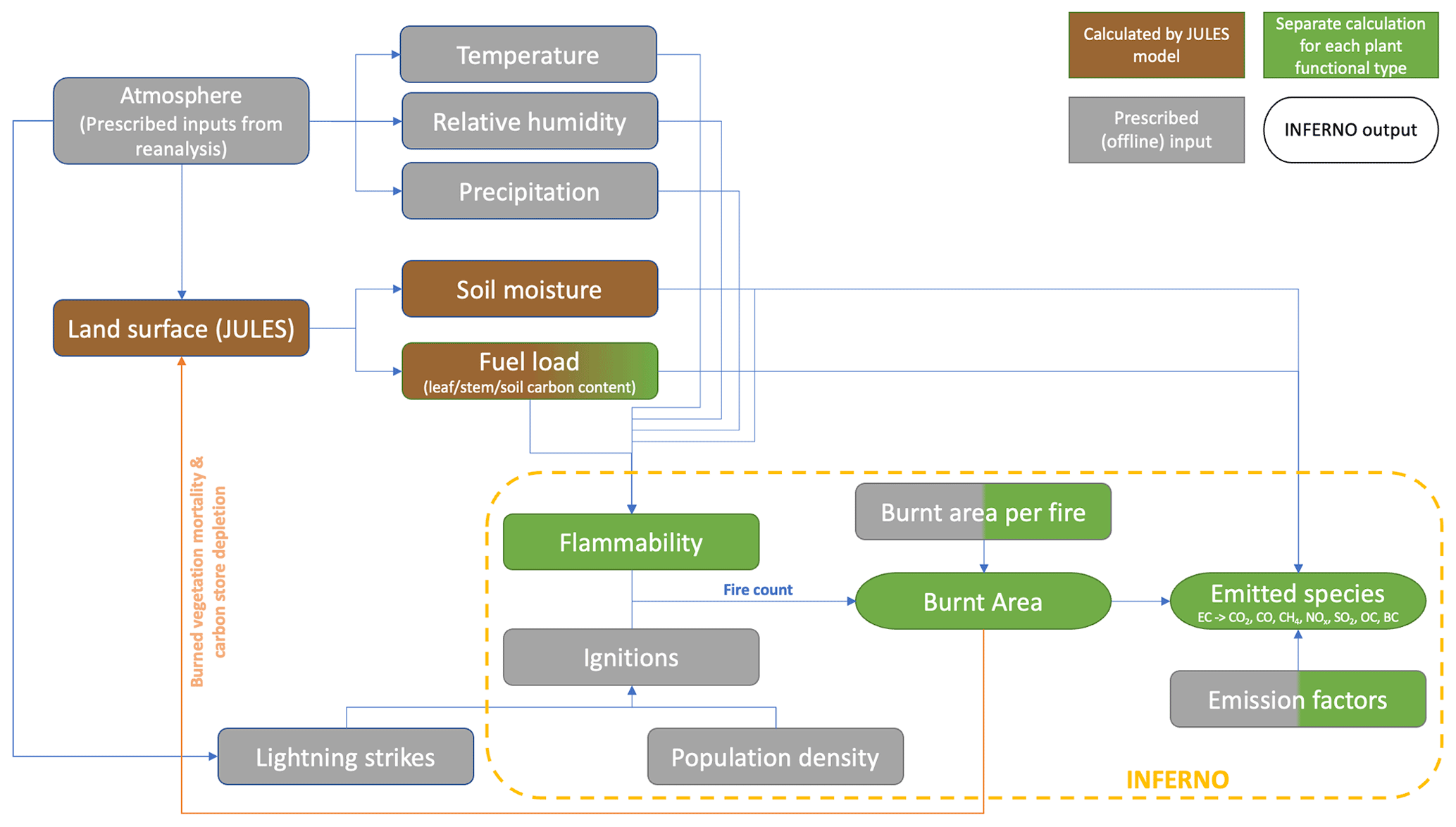
The Joint UK Land Environment Simulator (JULES) is simulating land surface vegetation, carbon stores, and hydrology, primarily using physical models to simulate the processes of land use, water and carbon fluxes with the atmosphere, and climate interactions with vegetation dynamics (Best et al., 2011; Clark et al., 2011). The INFERNO fire scheme was constructed based on a simplified parameterization of fire ignition and vegetation flammability (Pechony and Shindell, 2009). Coupled with JULES, the INFERNO scheme predicts fire burnt area and carbon emissions based on the simulated vegetation, as well as vegetation mortality due to fire, which feeds back on the vegetation distribution (Burton, 2019; Mangeon et al., 2016). More precisely, the model calculates flammability based on soil moisture, fuel density, temperature, humidity, and precipitation and then combines lightning strikes to estimate the average area burnt. Finally, emitted atmospheric aerosols and trace gases can be calculated from vegetation-dependent emission factors (Mangeon et al., 2016). Figure 1 illustrates the input variables and critical components of JULES-INFERNO. However, this model involves a large amount of data and number of parameters, leading to high computational cost. In the present paper, we propose the use of a surrogate model as a substitute for the original high-precision simulation model. The surrogate model aims to use the same input fields as the original model and to output a result that approximates the original INFERNO burnt area output but is less computationally intensive to solve.

Figure 1 The mechanism of JULES-INFERNO.

This research considered four meteorological boundary conditions and predicted burnt area (temperature (T), humidity (H), rainfall (R), and lightning (L)) and the field of burnt area fraction (P) from the JULES-INFERNO model as input data. We used an ensemble of five JULES-INFERNO simulations which were forced using meteorological conditions from the Fire Modeling Intercomparison Project (FireMIP) last glacial maximum (LGM) scenario (Rabin et al., 2017), which uses a detrended 1961–1990 re-analysis time series, uniformly shifted to match LGM global average climate, as the atmospheric boundary conditions. Monthly-mean values were collected for each meteorological boundary condition, nominally from 1961–1990 for each simulation. Thus 360 snapshots for each variable are available, denoted as temperature ($T_i,i=\mathrm{1},\mathrm{2},\mathrm{\cdots },\mathrm{360}$), humidity ($H_i,i=\mathrm{1},\mathrm{2},\mathrm{\cdots },\mathrm{360}$), rainfall ($R_i,i=\mathrm{1},\mathrm{2},\mathrm{\cdots },\mathrm{360}$), and lightning ($L_i,i=\mathrm{1},\mathrm{2},\mathrm{\cdots },\mathrm{360}$). JULES-INFERNO was run with a resolution of 1.25^∘ latitude × 1.875^∘ longitude, giving each snapshot a latitude span of 144 units and a longitude span of 192 units, so the size of each snapshot is 144×192. We denote the wildfire burnt area predicted by JULES-INFERNO from each of the five ensemble members as $P_{\mathrm{s}},s=\mathrm{1},\mathrm{2},\mathrm{\cdots },\mathrm{5})$. Although each ensemble member simulated the same nominal period (1961 to 1990) and was forced by the same detrended meteorological boundary conditions, we applied different initial internal states to sample a range of model internal variability. As shown in Table 1, P₁ was randomized, and the initial internal states of the subsequent experimental results were all the last internal states of the previous one. The burnt area model output is only diagnosed over latitudes with non-zero land cover, and so the wildfire burnt area data ($P_{\mathrm{s},i},s=\mathrm{1},\mathrm{2},\mathrm{\cdots },\mathrm{5},i=\mathrm{1},\mathrm{2},\mathrm{\cdots },\mathrm{360}$) only spans 112 latitude units, meaning the fire snapshot size is 112×192 rather than 144×192.

Table 1 JULES-INFERNO experiments' initial internal states.

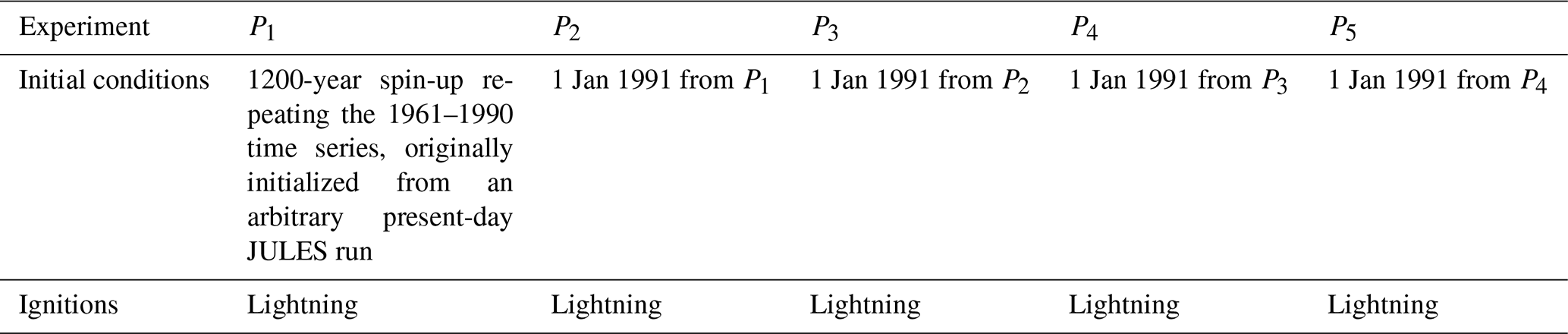
In subsequent experiments, P₁,P₂, and portion of P₃ are the training set, and another portion of P₃ is the validation set during training. P₄ and P₅ were used as the test set for all models built in the study. In addition, to eliminate the adverse effects of odd sample data in training, this research standardized all training and test sets (climates and fire variables) by applying Eq. (1) to normalize the data to [0, 1]:

$$\begin{array}{}\text{(1)}& P_{\mathrm{s}}={\displaystyle \frac{P_{\mathrm{s}}-P_{{\mathrm{s}}_{\min }}}{P_{{\mathrm{s}}_{\max }}-P_{{\mathrm{s}}_{\min }}}}s=\mathrm{1},\mathrm{2},\mathrm{\cdots },\mathrm{5}.\end{array}$$

3 Methodology

In this section, we present the main technologies used to develop the digital twin: ROM, surrogate predictive model, and LA. The computation of the digital twin starts by constructing the ROM for reducing the dimension of JULES-INFERNO data. The climate and wildfire data are then concatenated and processed into time series data and fed into the training predictive model. Afterwards, iterative forecasting tests the trained surrogate model. The test uses 12 months of unseen data as input to predict fires for the next 29 years. LA periodically adjusts the forecasting process to ensure stability, accuracy, and sustainability.

3.1 Reduced-order modelling

Assume that the original data are an n-dimensional vector denoted as $U=\mathit{\{}{u}_i{\mathit{\}}}_{i=\mathrm{1},\mathrm{2},\mathrm{\cdots },n}$; we then denote the compressed variable (k-dimension, k < n) after dimensionality reduction as $\stackrel{\mathrm{̃}}{U}=\mathit{\{}{\stackrel{\mathrm{̃}}{u}}_i{\mathit{\}}}_{i=\mathrm{1},\mathrm{2},\mathrm{\cdots },k}$. The variable that reconstructs the compressed data to the original size is denoted as $\widehat{U}=\mathit{\{}\widehat{u_i}{\mathit{\}}}_{i=\mathrm{1},\mathrm{2},\mathrm{\cdots },n}$. ROM's primary purpose is to minimize the expectation of the mean square error (MSE) of reconstruction, i.e. $E\left[\right(U-\widehat{U}{)}^{\mathrm{2}}]$. The meteorological boundary conditions and burnt area data obtained by dimensionality reduction can therefore be denoted by $\stackrel{\mathrm{̃}}{T_i},\stackrel{\mathrm{̃}}{H_i},\stackrel{\mathrm{̃}}{R_i},\stackrel{\mathrm{̃}}{L_i},\stackrel{\mathrm{̃}}{P_{\mathrm{s},i}},s=\mathrm{1},\mathrm{2},\mathrm{\cdots }\mathrm{5};i=\mathrm{1},\mathrm{2},\mathrm{\cdots }\mathrm{360}$, and each reduced snapshot is k-dimensional. Decoded data are denoted as $\widehat{T_i},\widehat{H_i},\widehat{R_i},\widehat{L_i},\widehat{P_{\mathrm{s},i}},s=\mathrm{1},\mathrm{2},\mathrm{\cdots }\mathrm{5};i=\mathrm{1},\mathrm{2},\mathrm{\cdots }\mathrm{360}$, and the dimensionality of each element is consistent with the original data (n-dimension).

3.1.1 PCA

PCA extracts essential information from the data and eliminates redundant information by analysing principal components. PCA uses the idea of dimensionality reduction to form new variables by linearly combining multiple parameter indicators and mapping the original n-dimensional features to k-dimensional features (n > k); k is known as the truncation parameter in PCA (Bianchi et al., 2015).

The compressed variable ${\stackrel{\mathrm{̃}}{u}}_i$ can be represented by a linear combination of $u_{\mathrm{1}},u_{\mathrm{2}},\mathrm{\dots },u_n$ as shown in Eq. (2) to make the global variance after the transformation maximal:

$$\begin{array}{}\text{(2)}& \left\{\begin{array}{l}{\stackrel{\mathrm{̃}}{u}}_{\mathrm{1}}={\mathit{\alpha }}_{\mathrm{11}}{u}_{\mathrm{1}}+{\mathit{\alpha }}_{\mathrm{12}}{u}_{\mathrm{2}}+\mathrm{\cdots }+{\mathit{\alpha }}_{\mathrm{1}n}{u}_n\\ {\stackrel{\mathrm{̃}}{u}}_{\mathrm{2}}={\mathit{\alpha }}_{\mathrm{21}}{u}_{\mathrm{1}}+{\mathit{\alpha }}_{\mathrm{22}}{u}_{\mathrm{2}}+\mathrm{\cdots }+{\mathit{\alpha }}_{\mathrm{2}n}{u}_n\\ {\stackrel{\mathrm{̃}}{u}}_{\mathrm{3}}={\mathit{\alpha }}_{\mathrm{31}}{u}_{\mathrm{1}}+{\mathit{\alpha }}_{\mathrm{32}}{u}_{\mathrm{2}}+\mathrm{\cdots }+{\mathit{\alpha }}_{\mathrm{3}n}{u}_n\\ \mathrm{⋮}\\ {\stackrel{\mathrm{̃}}{u}}_k={\mathit{\alpha }}_{k\mathrm{1}}{u}_{\mathrm{1}}+{\mathit{\alpha }}_{k\mathrm{2}}{u}_{\mathrm{2}}+\mathrm{\cdots }+{\mathit{\alpha }}_{kn}{u}_n\end{array}\right.,\end{array}$$

where ${\mathit{\alpha }}_i=[{\mathit{\alpha }}_{i\mathrm{1}},{\mathit{\alpha }}_{i\mathrm{1}},\mathrm{\cdots },{\mathit{\alpha }}_{\mathrm{in}}{]}^T(i=\mathrm{1},\mathrm{2},\mathrm{\cdots },k)$ is the eigenvector associated with the eigenvalues λ_i of the covariance matrix C.

The covariance matrix C is shown in Eq. (3), and the formula for the covariance is shown in Eq. (4):

$$\begin{array}{}\text{(3)}& {\displaystyle }\mathbf{C}=\left[\begin{array}{ccc}\begin{array}{cc}\mathrm{cov}\left(u_{\mathrm{1}},u_{\mathrm{1}}\right)& \mathrm{cov}\left(u_{\mathrm{1}},u_{\mathrm{2}}\right)\end{array}& \mathrm{\cdots }& \mathrm{cov}\left(u_{\mathrm{1}},u_n\right)\\ \mathrm{⋮}& \mathrm{\ddots }& \mathrm{⋮}\\ \begin{array}{cc}\mathrm{cov}\left(u_n,u_{\mathrm{1}}\right)& \mathrm{cov}\left(u_n,u_{\mathrm{2}}\right)\end{array}& \mathrm{\cdots }& \mathrm{cov}\left(u_n,u_n\right)\end{array}\right],\text{(4)}& {\displaystyle }\mathrm{cov}\left(u_i,u_j\right)=E\left(u_i{u}_j\right)-E\left(u_i\right)E\left(u_j\right)i,j=\mathrm{1},\mathrm{2},\mathrm{\cdots },n,\end{array}$$

where E(u_i) represents the mathematical expectation of u_i.

The contribution rate of each principal component can be calculated using the principal component explained variance formula (Eq. 5), and the principal components corresponding to the special eigenvalues ${\mathit{\lambda }}_{\mathrm{1}},{\mathit{\lambda }}_{\mathrm{2}},\mathrm{\cdots },{\mathit{\lambda }}_n$ are selected in descending order to construct $\stackrel{\mathrm{̃}}{U}$. The cumulative explained variance is referred to in Eq. (6):

$$\begin{array}{}\text{(5)}& {\displaystyle }{\mathit{\alpha }}_i={\displaystyle \frac{{\mathit{\lambda }}_i}{{\sum }_{j=\mathrm{1}}^k{\mathit{\lambda }}_j}},i,j=\mathrm{1},\mathrm{2},\mathrm{\cdots },k,\text{(6)}& {\displaystyle }{\sum }_{i=\mathrm{1}}^k{\mathit{\alpha }}_i={\displaystyle \frac{{\sum }_{j=\mathrm{1}}^k{\mathit{\lambda }}_j}{{\sum }_{j=\mathrm{1}}^k{\mathit{\lambda }}_j}},i,j=\mathrm{1},\mathrm{2},\mathrm{\cdots },k.\end{array}$$

3.1.2 CAE

An autoencoder (AE) is a self-supervised deep learning method that minimizes the reconstruction error between its model input and output. The autoencoder optimizes parameters to obtain a low-dimensional data representation of high-dimensional features (Huang et al., 2017). The feature extraction method used in standard AE is fully connected and straightforward to implement. However, each neuron connects to all the neurons in the next layer. Thus, standard AE generates massive parameters, making the computation more expensive while ignoring some spatial patterns in the image (Masci et al., 2011). A convolutional autoencoder (CAE) (Masci et al., 2011), a combination of AE and convolutional neural network (CNN), has been proposed to address the drawbacks of fully connected AEs. The CAE model inherits the self-supervision function of standard AE but replaces the matrix product operation between hidden neurons with convolution and pooling operations. Compared to AE, CAE can capture local spatial patterns of monitoring data (Masci et al., 2011). Furthermore, extracting features by convolution can reduce the number of parameters and increase the training speed.

This study includes climate and fire conditions from various regions in the form of 2-dimensional images. Therefore, this research constructed a CAE model using AE reconstruction, dimensionality reduction features, and CNN local-feature extraction capabilities. The CAE model aims to achieve self-supervised learning of environmental and wildfire features.

The encoder designed for this study uses three convolutional layers, three max pooling layers, and two fully connected layers. The decoder includes four convolutional layers, three up-sampling layers, and one fully connected layer. Figure 2 shows the CAE structure of this study with a latent space of dimension 100 and with Conv2d, MaxPooling2D, Dense, and UpSampling2D representing the 2D convolutional layer, max pooling layer, fully connected layer, and up-sampling layer respectively.

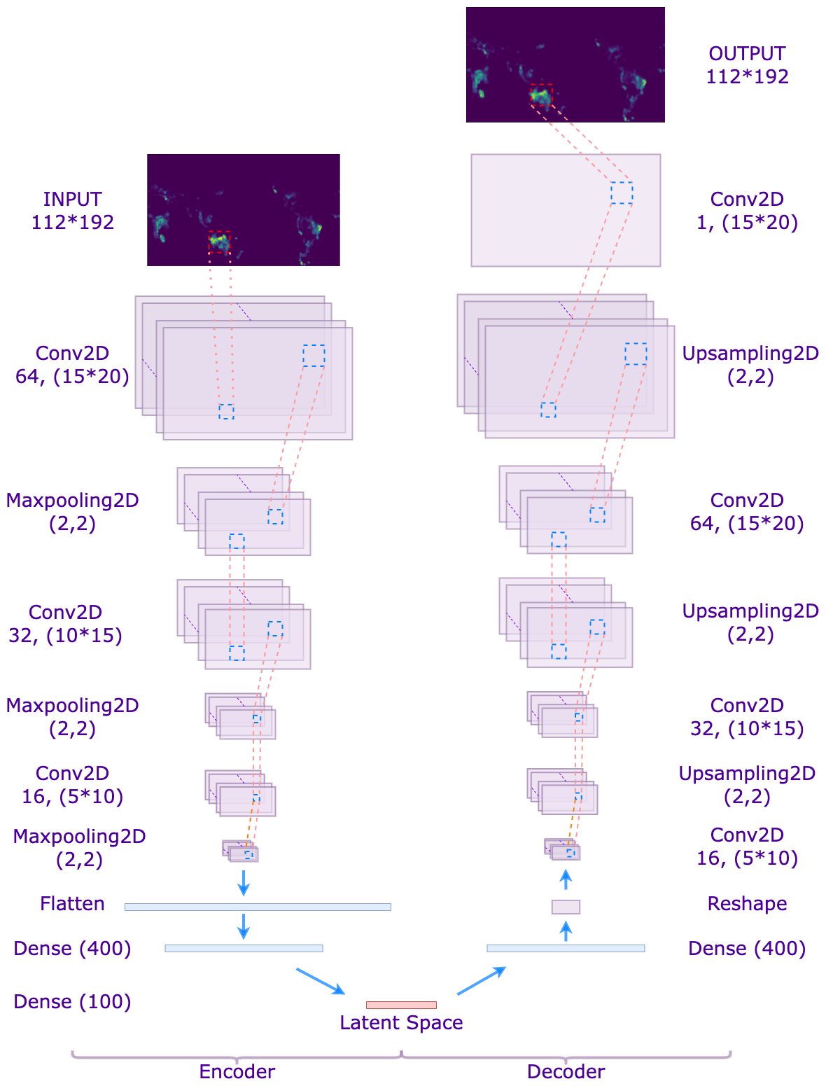
Figure 2 The CAE model structure.

Firstly, the sample data, $U=\mathit{\{}{u}_i{\mathit{\}}}_{i=\mathrm{1},\mathrm{2},\mathrm{\cdots },n}$, need to be converted into a 2-dimensional matrix of p rows and q columns ($p\cdot q=n$) according to the latitude and longitude range of the original data, and then each snapshot could be interpreted as an image. Given the input U, features are extracted by multiple convolutional kernels to obtain the output C_l of the lth layer, and then the $C_l^{\prime }$ is obtained by down-sampling through the subsequent pooling layer to retain the main features of the inflow data and prevent over-fitting. The operational methods are shown in Eqs. (7) and (8):

$$\begin{array}{}\text{(7)}& {\displaystyle }\left\{\begin{array}{ll}{C}_l=f\left(W_l\otimes U+b_l\right),& l=\mathrm{1}\\ C_l=f\left(W_l\otimes C_{l-\mathrm{1}}^{\prime }+b_l\right),& l=\mathrm{2},\mathrm{3},\end{array}\right.\text{(8)}& {\displaystyle }\begin{array}{ll}{C}_{l-\mathrm{1}}^{\prime }=\mathrm{Maxpooling}\left(C_l\right),& l=\mathrm{1},\mathrm{2},\mathrm{3},\end{array}\end{array}$$

where W_l and b_l are the weights and biases of the layer l network respectively, f(⋅) is the rectified linear unit (ReLU) function, and Maxpooling(⋅) is the maximum pooling operation.

As shown in Fig. 2, during the network training process, the encoder acquires the feature mapping of the input data layer by layer. It obtains the k-dimensional latent space data after the flatten and dense layers. In contrast, the decoder inputs the latent space data and reconstructs the data by convolution, up-sampling, etc., and evaluates the reconstruction performance of CAE on climate and wildfire data by the loss function (MSE). Equation (9) shows the square error of one sample (L(⋅)) and mean error for the training set (J(⋅)), supposing the training set is P_tr with N_tr snapshots:

$$\begin{array}{}\text{(9)}& \left\{\begin{array}{l}L(U,\widehat{U})=(U-\widehat{U}{)}^{\mathrm{2}}\\ J(P_{\mathrm{tr}},\widehat{P_{\mathrm{tr}}})=\frac{\mathrm{1}}{N_{\mathrm{tr}}}{\sum }_{i=\mathrm{1}}^{N_{\mathrm{tr}}}L(P_{\mathrm{tr},\mathrm{i}},\widehat{P_{\mathrm{tr},\mathrm{i}}})\end{array}.\right.\end{array}$$

3.2 Surrogate predictive model

After data compression, the proposed digital twin model combined the climate and fire data as inputs for the predictive surrogate model, denoted as $Z={\left\{Z_{\mathrm{s}}\right\}}_{\mathrm{s}=\mathrm{1},\mathrm{2},\mathrm{\cdots }\mathrm{5}}$ and $Z_{\mathrm{s}}={\left\{Z_{\mathrm{s},i}\right\}}_{\mathrm{s}=\mathrm{1},\mathrm{2},\mathrm{\cdots }\mathrm{5};i=\mathrm{1},\mathrm{2},\mathrm{\cdots }\mathrm{360}}=\left[\stackrel{\mathrm{̃}}{P_{\mathrm{s},i}}\stackrel{\mathrm{̃}}{T_i}\stackrel{\mathrm{̃}}{H_i}\stackrel{\mathrm{̃}}{R_i}\stackrel{\mathrm{̃}}{L_i}\right]$, where “s=1, 2,..5” indicates the five fire respective datasets (i.e. JULES-INFERNO simulations). The data are normalized before being fed into the model.

Here we aim to use ML techniques to surrogate the original physical predictive model. The recurrent neural network (RNN) is a reference method for time series prediction problems. The LSTM network, a variant of RNN, constructed the wildfire predictive model in the reduced latent space using the encoded JULES-INFERNO climate and fire data as inputs. Figure 3 shows the basic structure of the whole surrogate model.

Figure 3 The surrogate model structure.

The seq2seq prediction based on the LSTM network is implemented in this study with t_in time steps as input and t_out time steps as output. Here, each time step represents a month of simulation time. The length of the input and output sequences is fixed as $t_{\mathrm{in}}=t_{\mathrm{out}}=\mathrm{12}\mathrm{\dots }{Z}_{\mathrm{train}}=Z_{\mathrm{1}}\bigcup Z_{\mathrm{2}}\bigcup Z_{\mathrm{3}}$, and the test set consists of $Z_{\mathrm{test}}=Z_{\mathrm{4}}\bigcup Z_{\mathrm{5}}$. The input of the LSTM training can be obtained by shifting the initial time of each time series, as shown in Eq. (10). The model uses MSE loss function to evaluate the training performance:

$$\begin{array}{}\text{(10)}& \begin{array}{rl}& [Z_{\mathrm{1},\mathrm{1}},Z_{\mathrm{1},\mathrm{2}},\mathrm{\cdots },Z_{\mathrm{1},t_{\mathrm{in}}}]\\ & \stackrel{\mathrm{LSTM}\mathrm{train}}{⟶}[Z_{\mathrm{1},t_{\mathrm{in}}+\mathrm{1}},Z_{\mathrm{1},t_{\mathrm{in}}+\mathrm{2}},\mathrm{\cdots },Z_{\mathrm{1},t_{\mathrm{in}}+t_{\mathrm{out}}}],\\ & [Z_{\mathrm{1},\mathrm{2}},Z_{\mathrm{1},\mathrm{3}},\mathrm{\cdots },Z_{\mathrm{1},t_{\mathrm{in}}+\mathrm{1}}]\\ & \stackrel{\mathrm{LSTM}\mathrm{train}}{⟶}[Z_{\mathrm{1},t_{\mathrm{in}}+\mathrm{2}},Z_{\mathrm{1},t_{\mathrm{in}}+\mathrm{3}},\mathrm{\cdots },Z_{\mathrm{1},t_{\mathrm{in}}+t_{\mathrm{out}}+\mathrm{1}}]\\ & \mathrm{⋮}\\ & [Z_{\mathrm{1},\mathrm{360}-t_{\mathrm{in}}-t_{\mathrm{out}}+\mathrm{1}},\mathrm{\cdots },Z_{\mathrm{1},\mathrm{360}-t_{\mathrm{out}}}]\\ & \stackrel{\mathrm{LSTM}\mathrm{train}}{⟶}[Z_{\mathrm{1},\mathrm{360}-t_{\mathrm{out}}+\mathrm{1}},Z_{\mathrm{1},\mathrm{360}-t_{\mathrm{out}}+\mathrm{2}},\mathrm{\cdots },Z_{\mathrm{1},\mathrm{360}}]\\ & \mathrm{⋮}\\ & [Z_{\mathrm{3},\mathrm{360}-t_{\mathrm{in}}-t_{\mathrm{out}}+\mathrm{1}},\mathrm{\cdots },Z_{\mathrm{3},\mathrm{360}-t_{\mathrm{out}}}]\\ & \stackrel{\mathrm{LSTM}\mathrm{train}}{⟶}[Z_{\mathrm{3},\mathrm{360}-t_{\mathrm{out}}+\mathrm{1}},Z_{\mathrm{3},\mathrm{360}-t_{\mathrm{out}}+\mathrm{2}}\mathrm{\cdots },Z_{\mathrm{3},\mathrm{360}}].\end{array}\end{array}$$

As for the iterative predictions in the test dataset, the trained model uses the current predictive result as the input of the next prediction. The output of the predictive model can be denoted as $Z_{\mathrm{test}}^{\prime }=Z_{\mathrm{4}}^{\prime }\cup Z_{\mathrm{5}}^{\prime }$. The first-year data of the test set is used as model input, and the prediction result set only contains data from the following 29 years. At each iteration, the model can predict the global wildfire risk for the next year, as shown in Eq. (11):

$$\begin{array}{}\text{(11)}& \begin{array}{rl}& [Z_{\mathrm{4},\mathrm{1}},Z_{\mathrm{4},\mathrm{2}},\mathrm{\cdots },Z_{\mathrm{4},\mathrm{12}}]\stackrel{\mathrm{LSTM}\mathrm{predict}}{⟶}[Z_{\mathrm{4},\mathrm{13}}^{\prime },Z_{\mathrm{4},\mathrm{14}}^{\prime },\mathrm{\cdots },Z_{\mathrm{4},\mathrm{24}}^{\prime }],\\ & [Z_{\mathrm{4},\mathrm{13}}^{\prime },Z_{\mathrm{4},\mathrm{14}}^{\prime },\mathrm{\cdots },Z_{\mathrm{4},\mathrm{24}}^{\prime }]\\ & \stackrel{\mathrm{LSTM}\mathrm{predict}}{⟶}[Z_{\mathrm{4},\mathrm{25}}^{\prime },Z_{\mathrm{4},\mathrm{26}}^{\prime },\mathrm{\cdots },Z_{\mathrm{4},\mathrm{36}}^{\prime }]\\ & \mathrm{⋮}\\ & [Z_{\mathrm{4},\mathrm{337}}^{\prime },Z_{\mathrm{4},\mathrm{338}}^{\prime },\mathrm{\cdots },Z_{\mathrm{4},\mathrm{348}}^{\prime }]\\ & \stackrel{\mathrm{LSTM}\mathrm{predict}}{⟶}[Z_{\mathrm{4},\mathrm{349}}^{\prime },Z_{\mathrm{4},\mathrm{350}}^{\prime },\mathrm{\cdots },Z_{\mathrm{4},\mathrm{360}}^{\prime }],\\ & [Z_{\mathrm{5},\mathrm{1}},Z_{\mathrm{5},\mathrm{2}},\mathrm{\cdots },Z_{\mathrm{5},\mathrm{12}}]\\ & \stackrel{\mathrm{LSTM}\mathrm{predict}}{⟶}[Z_{\mathrm{5},\mathrm{13}}^{\prime },Z_{\mathrm{5},\mathrm{14}}^{\prime },\mathrm{\cdots },Z_{\mathrm{5},\mathrm{24}}^{\prime }]\\ & \mathrm{⋮}\\ & [Z_{\mathrm{5},\mathrm{337}}^{\prime },Z_{\mathrm{5},\mathrm{338}}^{\prime },\mathrm{\cdots },Z_{\mathrm{5},\mathrm{348}}^{\prime }]\\ & \stackrel{\mathrm{LSTM}\mathrm{predict}}{⟶}[Z_{\mathrm{5},\mathrm{349}}^{\prime },Z_{\mathrm{5},\mathrm{350}}^{\prime },\mathrm{\cdots },Z_{\mathrm{5},\mathrm{360}}^{\prime }].\end{array}\end{array}$$

Thanks to the gate structure, LSTM networks are efficient in dealing with long-term temporal correlations that standard RNNs cannot handle (Graves and Schmidhuber, 2005b). More precisely, the essence of the gate structure of the LSTM is to use the sigmoid activation function so that the fully connected network layer outputs a value between 0 and 1, describing the proportion of the information quantity passed. The forget gate indicates the proportion of the output information quantity forgotten at the last moment, and the input gate represents the proportion of the input information quantity retained at the current moment, both updating the state value together. Finally, the output gate represents the proportion of the new state output. Suppose x_t ($x_{\mathrm{0}}=[Z_{\mathrm{s},i},Z_{\mathrm{s},i+\mathrm{1}},\mathrm{\cdots },Z_{\mathrm{s},i+t_{\mathrm{in}}-\mathrm{1}}]$, $s=\mathrm{1},\mathrm{2},\mathrm{3},i=\mathrm{1},\mathrm{2},\mathrm{\cdots },\mathrm{349}$) are the current inputs, h_t−1 is the output of last moment, c_t is the value of the new state, and c_t−1 is the state value of last moment. Equations (12), (13), (14), (15), (16), and (17) represent the inner principal of the LSTM:

$$\begin{array}{}\text{(12)}& {\displaystyle }\text{Input state:}{z}_t=\tanh \left(W_z{x}_t+Q_z{h}_{t-\mathrm{1}}+b_z\right),\text{(13)}& {\displaystyle }\text{Input gate:}{i}_t=\mathit{\sigma }\left(W_i{x}_t+Q_i{h}_{t-\mathrm{1}}+b_i\right),\text{(14)}& {\displaystyle }\text{Forget gate:}{f}_t=\mathit{\sigma }\left(W_f{x}_t+Q_f{h}_{t-\mathrm{1}}+b_f\right),\text{(15)}& {\displaystyle }\text{Current state:}{c}_t=f_t\cdot c_{t-\mathrm{1}}+i_t\cdot z_t,\text{(16)}& {\displaystyle }\text{Output gate:}{o}_t=\mathit{\sigma }\left(W_o{x}_t+Q_o{h}_{t-\mathrm{1}}+b_o\right),\text{(17)}& {\displaystyle }\text{Current output:}{h}_t=o_t\cdot \tanh \left(c_t\right),\end{array}$$

where $W_z,W_i,W_f$, and W_o are input weighting matrix; $Q_z,Q_i,Q_f$, and Q_o are loop weights; $b_z,b_i,b_f$, and b_o are bias values; and σ(⋅) is the sigmoid function.

3.3 Latent data assimilation

The basic principle of DA is the combination of numerical models with observation data to improve the forecast of the system under study (Vallino, 2000). When applying the developed predictive model to unseen initial conditions, we apply the DA method periodically to enhance the current prediction results with the help of the observation data. The observation data in this research is considered the original output of the JULES-INFERNO model so that we can simulate the situation where high-quality real-time observation data are available. As periodic corrections are made to the forecast data, DA allows for a more stable and accurate long-term prediction. In this study, LA was applied, which combines ROM with DA, i.e. reducing the dimensionality of the data before applying the DA method (Peyron et al., 2021). In addition, ROM could reduce the parameters for subsequent operations, which allows LA to have a significant advantage in terms of computational efficiency compared to the classical full-space DA.

Both DA and LA can be summarized as a problem of solving the minimization of an objective function J_DA(⋅) characterizing the deviation between the analysis field (optimal state ${\dot{Z}}_{\mathrm{test}}$) and the observation field (actual state Z_test), as well as the background field (predicted state $Z_{\mathrm{test}}^{\prime }$), as shown in Eq. (18):

$$\begin{array}{}\text{(18)}& \begin{array}{rl}{J}_{\mathrm{DA}}\left(\dot{z_t}\right)& ={\displaystyle \frac{\mathrm{1}}{\mathrm{2}}}{\left(\dot{z_t}-z_t^{\prime }\right)}^T{\mathrm{B}}^{-\mathrm{1}}\left(\dot{z_t}-z_t^{\prime }\right)\\ & +{\displaystyle \frac{\mathrm{1}}{\mathrm{2}}}{\left[z_t-H\left(\dot{z_t}\right)\right]}^T{\mathrm{O}}^{-\mathrm{1}}\left[z_t-H\left(\dot{z_t}\right)\right],\end{array}\end{array}$$

where t indicates the temporal index (the tth predicted year), $\dot{z_t}$ is the analysis variable of DA, $z_t^{\prime }$ is the background variable, and z_t is the observation (original) variable. B and O represent the background and observation error covariance matrix. The modelling of these covariances determines the weight of prediction and observation in the objective function, which is crucial for DA approaches (Lawless et al., 2005). H(⋅) is the state-observation function in latent space, which maps the analysis variable to the observation variable. In this study, since we are assimilating the compressed output of the original JULES-INFERNO model, H(⋅) is the identity function.

The latent analysis field ${\dot{Z}}_{\mathrm{test},t}$ could be obtained by optimizing the objective function (Eq. 18):

$$\begin{array}{}\text{(19)}& {\dot{Z}}_{\mathrm{test},t}=\mathrm{argmin}\left(J_{\mathrm{DA}}\left(\dot{z_t}\right)\right).\end{array}$$

Equation (18) can be solved by the best linear unbiased estimator (Fulton, 2000), since the transformation operator H=H is a linear function in the latent space:

$$\begin{array}{}\text{(20)}& {\dot{Z}}_{\mathrm{test},t}=z_t^{\prime }+B{H}^T{\left(HB{H}^T+O\right)}^{-\mathrm{1}}\left(z_t-H\left(z_t^{\prime }\right)\right).\end{array}$$

The obtained analysis state ${\dot{Z}}_{\mathrm{test},t}$ can be used as an initial point for the next-level prediction, as shown in Fig. 4, and the predicted field in the latent space could be ${\dot{Z}}_{\mathrm{test},t}$ (when applying LA at t time index) or $Z_{\mathrm{test},t}^{\prime }$ (LSTM prediction at t time index). These processes can be repeated periodically to consistently improve the prediction performance. Furthermore, in Fig. 4, the final predicted sequence of the digital twin is the combination of $\mathit{\{}{\dot{Z}}_{\mathrm{test},t}{\mathit{\}}}_{n\mathit{ϵ}[\mathrm{0},\mathrm{29}]}$ and $\mathit{\{}{Z}_{\mathrm{test},m}^{\prime }{\mathit{\}}}_{m\in [\mathrm{0},\mathrm{29}]}$ (m≠n), which could be denoted as $Z_{\mathrm{opt}}^{\prime }$.

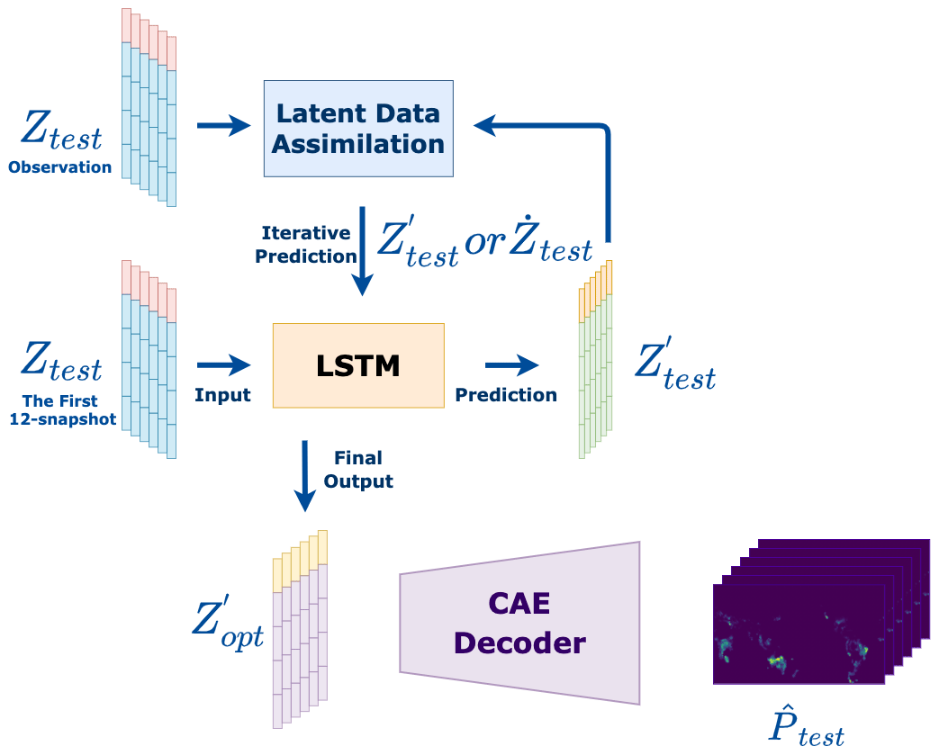
Figure 4 The predictive model with LA.

4 Numerical results

In this section, we evaluate the proposed digital twin model's performance regarding prediction accuracy and computational efficiency when the digital twin model faces unseen initial conditions.

4.1 ROM results

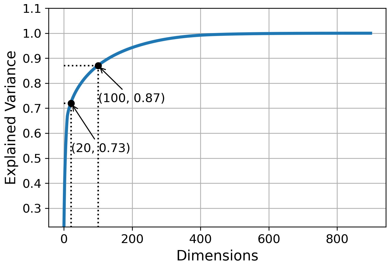
To set an optimal dimension of the latent space, we examined the explained variance of PCA for the training dataset. The training dataset consists of P₁, P₂, and P₃ with different numbers of principal components, as shown in Fig. 5. According to the work of Li et al. (2021), 85 % to 95 % of the explained variance can reflect most data information while effectively reducing the original data dimensionality. Therefore, to reduce the latent space dimension and the computational cost of subsequent processing, we chose in this research the 100-dimension latent space with 87 % explained variance, as shown in Fig. 5. In addition, we also chose the 20-dimensional latent space for both PCA and CAE for comparison purposes.

Figure 5 PCA-explained variances with different dimensions.

In terms of performance evaluation, the scenarios $P_{\mathrm{1}}\cup P_{\mathrm{2}}\cup P_{\mathrm{3}}$ are used as the training set and P₄ ∪ P₅ are considered as the test set. The number of training epochs for the CAE models is fixed at 1000. The MSEs between reconstructed and original simulations for different models are shown in Table 2. To quantify the mismatch between the JULES-INFERNO output P and decoded prediction P^′, we compute the MSE averaged by the number of pixels, i.e.

$${\in }^{\mathrm{MSE}}=\sqrt{\sum \mathrm{|}\mathrm{|}{P}_{i,j}-{P^{\prime }}_{i,j}\mathrm{|}{\mathrm{|}}_{\mathrm{2}}^{\mathrm{2}}}/(\mathrm{112}\cdot \mathrm{192}).$$

Table 2 PCA and CAE performances.

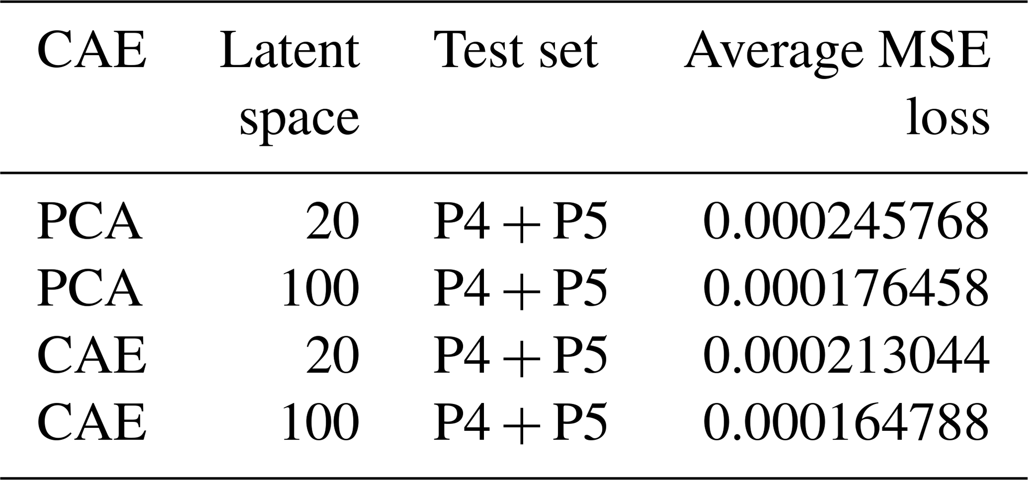
According to Table 2, for both PCA and CAE with 100-dimensional latent space, the reconstruction error is significantly lower compared to 20-dimensional. Furthermore, it can be evaluated from the experimental results that the CAE reconstruction MSE is lower compared to PCA. As previously described, CAE can capture feature information in 2-dimensional images during the encoding process, while PCA, which performs compression in 1-dimension space, may ignore these spatial patterns. In summary, CAE with 100-dimensional latent space has the best reconstruction performance in these experiments. As for the compression of climatic conditions $T,H,R$, and L, 83 % of data are used for PCA and CAE model training, and the rest of the data are used for model testing, where PCA and CAE have a similar performance.

4.2 Predictive model and latent data assimilation

After completing the ROM, the original JULES-INFERNO data are compressed into specific latent spaces, considerably reducing the number of parameters in the predictive model. The concatenated wildfire burnt area field and the four climate variables act as inputs to the surrogate model. Thus, the surrogate model achieves the same inputs as JULES-INFERNO. The predictive model (LSTM) trains separately using encoded data from different ROMs. Similar to the ROM, P₁, P₂, and P₃ are used as the training set, while P₄ and P₅ are used as the test set to evaluate the model performance. Each LSTM model has been trained over 10 000 epochs. As explained in Sect. 3.2, iterative predictions are used for the proposed digital twin. In other words, we first input the first year (12 snapshots) data and then use the current predicted result for the next-level prediction, until the 30th year's total burnt area is predicted. The MSEs for different combinations of ROM and LSTM are shown in Table 3.

Table 3 Surrogate models' performance.

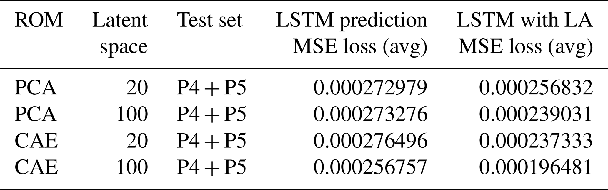
Table 3 shows that the predictions obtained using PCA down to 20 and 100 dimensions and CAE reduced to 20 dimensions are similar, with an MSE close to $\mathrm{2.7}\times {\mathrm{10}}^{-\mathrm{4}}$. Same as ROM, the best performance in LSTM prediction is obtained by applying CAE with 100-dimensional latent space, with an MSE loss of approximately $\mathrm{2.5}\times {\mathrm{10}}^{-\mathrm{4}}$.

Comparing the results shown in Tables 2 and 3, there is a gap between the MSE of the predictive model and the ROM reconstruction, mainly because of the accumulation of errors during the iterative prediction process. Therefore, we periodically used the observations (raw data) and LA to adjust the forecast results to stabilize subsequent forecasts. LA is implemented every 5 years during the prediction phase in this study. According to Table 3, there is a steady reduction in forecast MSE after correction by LA. The most significant reduction in MSE is obtained with 100-dimensional CAE compared to other approaches.

To better illustrate the evolution of the prediction error, we display the MSE of the prediction against time in different predictive models. In this study, the existing climate and fire data in 1961 (provided by JULES-INFERNO) with different initial conditions are given to predict the subsequent 29 years of fire. Figure 6 shows the MSE per prediction for the different surrogate models (in red when without LA and in green when with LA) evaluated on the P₄ test set, and we plotted the ROM MSE (in blue) for comparison.

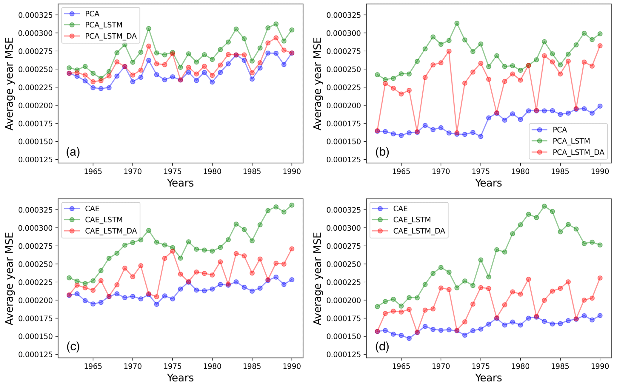
Figure 6 Evolution of MSE through the years in different surrogate models: (a) 20-dimensional PCA-based model, (b) 100-dimensional PCA-based model, (c) 20-dimensional CAE-based model, and (b) 100-dimensional CAE-based model.

According to Fig. 6, using LA can effectively reduce the prediction error, as the vast majority of red points are significantly lower than the corresponding green points. Furthermore, CAE-based surrogate models can better adapt the LA, stabilizing the predictions afterwards and reducing the accumulation of errors. When applying the LA to the PCA-based surrogate models to reduce the error after the simulation, there may still be a sharply increasing forecast error in the subsequent year, as seen in Fig. 6a and b. On the other hand, CAE-based models manage to maintain the improvement in DA for future time steps, as shown in Fig. 6c and d. These results demonstrate the advantage of CAE compared to PCA in terms of generalizability when applied to unseen data. This effect has also been highlighted in the work of Peyron et al. (2021). Comparing the four cases presented in Fig. 6, the 100-dimensional CAE demonstrates the strength of both the original prediction and the assimilated one.

Figure 7 The normalized output of 100-dimensional CAE-based digital twin: (a, b, c, d) the normalized output of original burnt area fraction, and their corresponding dates are January 1983, July 1983, January 1988, and July 1988; (e, f, g, h) the reconstructed output of the CAE model, and their corresponding dates are January 1983 , July 1983, January 1988, and July 1988; (i, j, k, l) the predicted output of CAE with the LSTM model, and their corresponding dates are January 1983, July 1983, January 1988, and July 1988; (m, n, o, p) the predicted output of CAE with the LSTM and LA models, and their corresponding dates are January 1983, July 1983, January 1988, and July 1988.

Figure 7 displays the output of the 100-dimensional CAE-based digital twin model of the years 1983 and 1988 (1 year after LA is implemented): the assimilated results (m, n, o, p) are compared with the original simulation (a, b, c, d), the CAE reconstruction (e, f, g, h), and the decoded image predicted by the LSTM model (i, j, k, l). In addition, the total burnt areas shown in Fig. 7 are normalized to the range 0 to 1. The horizontal and vertical coordinates in Fig. 7 represent latitude and longitude, and the colour values in the figure represent the grid box which indicates estimated burnt area fraction. The brighter the colour is, the larger the value is, and the colour bar is shown at the bottom of Fig. 7. It can be seen from Fig. 7 that forest wildfires in January are mainly in the Southern Hemisphere, such as Oceania (Fig. 7a) and South America in (Fig. 7c). On the other hand, the forest fires in July are mainly in the Northern Hemisphere, such as continental Europe in Fig. 7b and d.

As observed in Fig. 7, CAE and LSTM without LA can effectively reconstruct most of the features in the original image. Furthermore, comparing the LSTM-predicted images (i, j, k, l) and the optimization results after applying LA (m, n, o, p), it is found that the assimilation results are significantly closer to the JULES-INFERNO output.

Overall, in this research, we implemented four ROMs based on PCA and CAE, and the comparison reveals that the 100-dimensional CAE has the best reconstruction performance. Then, after combining the ROMs with predictive models (LSTM), a gap between the prediction results and the ROM reconstruction results is noticed. Eventually, the predictions of the surrogate model are made more stable after regular applications of LA to adjust the prediction outputs.

Table 4 compares the prediction time costs of the surrogate models using PCA and CAE downscaled to a 100-dimensional latent space without and with LA respectively. The prediction time of JULES-INFERNO in HPC is also shown as a reference. As can be seen in Table 4, the difference between PCA and CAE on the running time of the models is not significant; the application of LA slows down the prediction but still reduces the computing time cost significantly (around 500 times) compared to the original JULES-INFERNO fire predictive model.

Table 4 Time efficiency comparison.

In this study, the training of CAE and LSTM is performed with one NVIDIA P100 GPU (16 GB VRAM) in the Google Colab environment. All the online computations, including decoding, prediction and assimilation, are performed with Google Colab Intel CPUs as shown in Table 4. It is important to highlight that the application of such a digital twin does not require any HPC or GPU resources. Thus, a personal laptop can also run the model successfully.

5 Conclusion and future work

This study implemented a deep-learning-based digital twin for global wildfire prediction using the same input and output fields to replace the physical wildfire model JULES-INFERNO. The proposed model builds ROMs to encode the data into latent space to reduce subsequent processes' computational costs. Then it makes use of the compressed data to train a predictive model based on RNN. Finally, it applies LA to stabilize the prediction results when using the predictive model for iterative prediction to avoid error accumulation. According to the numerical results, the digital twin built using CAE is more accurate compared to the ones using PCA and can effectively capture the features of the original image for encoding and decoding. Applying LA periodically to optimize the prediction results can address the issue of error accumulation and achieve stable long-term predictions. Ultimately the research achieved a much more efficient wildfire-prediction digital twin based on JULES-INFERNO. The proposed model takes only 35 s on a laptop to predict 30 years of burnt area fractions, compared to ∼5 h using the original physical model on a 32-thread HPC node. The present research clearly brings additional insight to the computing of reduced-order digital twins for high-dimensional dynamical systems. Future work can consider further improving the generalizability of the proposed approach, by, for instance, training the model with scenarios of different time periods or fine tuning the model when the initial conditions are outside the range of the training set. In addition, it is reported in recent works (Teckentrup et al., 2019) that long-term predictions of JULES-INFERNO can introduce forecast bias. Further efforts can be considered to apply a latent data assimilation framework developed in this paper with real-time satellite observations.