the Creative Commons Attribution 4.0 License.
the Creative Commons Attribution 4.0 License.
 | 20 Apr 2023
The effect of deep ocean currents on ocean- bottom seismometers records
Afonso Loureiro
José Luis Duarte
Luis Matias
Tiago Rebelo
Tiago Bartolomeu
Ocean-bottom seismometers (OBSs) are usually deployed for seismological investigations, but these objectives are impaired by noise resulting from the ocean environment. We split the OBS-recorded seismic noise into three bands: short periods, microseisms and long periods, also known as tilt noise. We show that bottom currents control the first and third bands, but these are not always a function of the tidal forcing. Instead, we suggest that the ocean bottom has a flow regime resulting from two possible contributions: the permanent low-frequency bottom current and the tidal current. The recorded noise displays the balance between these currents along the entire tidal cycle, between neap and spring tides. In the short-period noise band, the ocean current generates harmonic tremors corrupting seismic dataset records. We show that, in the investigated cases, the harmonic tremors result from the interaction between the ocean current and mechanical elements of the OBS that are not essential during the sea bottom recording and thus have no geological origin. The data from a new broadband OBS type, designed and built at Instituto Dom Luiz (IDL – University of Lisbon)/Centre of Engineering and Product Development (CEIIA), hiding non-essential components from the current flow, show how utmost harmonic noise can be eliminated.
- Article
(13525 KB) - Full-text XML
-
Supplement
(41918 KB) - BibTeX
- EndNote


Ocean-bottom seismometers (OBSs) are deep-sea instruments that contain a three-component seismometer and a hydrophone built with the primary purpose of monitoring offshore seismicity of tectonically active areas (e.g. Geissler et al., 2010; Silva et al., 2017), contribute to regional and global seismology studies (e.g. Monna et al., 2014; Civiero et al., 2018, 2019) and image the marine subseafloor (e.g. Bowden et al., 2016; Loureiro et al., 2016; Corela et al., 2017). Typically, these instruments are dropped from a ship into the ocean and free fall through the water column until they reach the seafloor.
OBS measures ground motions, much like seismic stations on land do. However, deployment conditions on the seafloor differ from those on the continents as the seismometers can be protected from environmental disturbances (e.g. wind, temperature) through installations several metres underground. In contrast, in most cases, OBS stays on the seafloor and is exposed to all oceanic physical phenomena. This makes an OBS more than a seismic station, recording in addition to all types of seismic data (of geological, biological or anthropogenic origin) also oceanographic information (currents) as noise data. The noise of oceanic origin significantly impairs the investigation of all other phenomena leading to significant challenges and technical difficulties.
This noise can be split into three different bands in spectrograms (Fig. 1): (i) a subset of the short-period band from 0.5 to 6.5 Hz, the “harmonic tremors” (e.g. Díaz et al., 2007; Monigle et al., 2009) discussed and interpreted either as an instrumental cause, a geological cause or both; (ii) from 2 to 20 s, a well-known geophysical origin that corresponds to the microseismic band (Longuet-Higgins, 1950); and (iii) the long-period band from 20 to 60 s dominated by the tilt noise (Crawford and Webb, 2000), generally attributed to currents tilting the instrument.
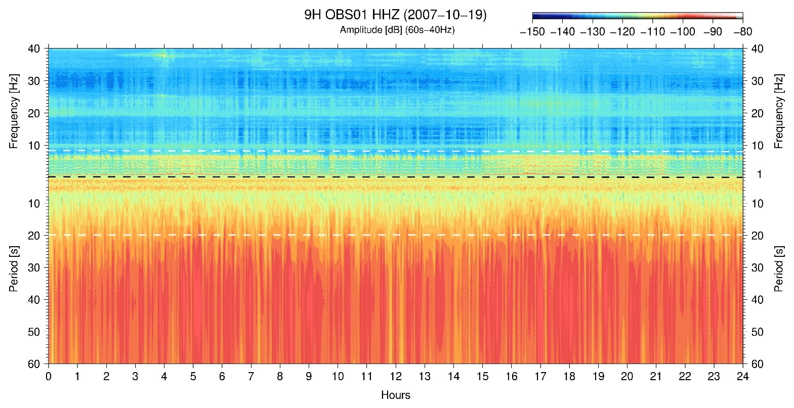
Figure 1Noise bands – inside the short-period band, from 0.5 to 6.5 Hz, we show long-lasting harmonic tremor signals frequently observed in spectrograms of OBS data with overlapping frequency content with earthquake detection events. The long-period band from the 20–60 s shows the tilt noise and the microseism noise band between 2 and 20 s. The harmonic tremors, microseism and tilt noise are shown in this particular OBS data record and are continuously observed in a one-day spectrogram (OBS01). The spectrogram is between 40 and 0.0167 Hz (60 s), however, between 1 and 0.0167 Hz converted to the period in seconds with linear axes. The amplitude unit is m2 s−4 Hz−1 [dB].
One of the challenges of seismic observations in the oceans regards the efficiency of noise reduction generated by oceanic processes (Webb, 1998). Therefore, understanding the sources and amplitudes of ocean seismic noise is essential for improving OBS design in terms of instrumental capabilities and noise mitigation.
On the short-period band (Fig. 1), 0.5–40 Hz (limited by the sampling rate of 100 Hz), local seismic events and whale vocalisations are widely recorded. Long-lasting harmonic tremor signals are commonly observed in spectrograms of OBS data with frequency content overlapping local earthquake signals. The resonance of OBS–sediment coupling could be generally observed in this same band of interest. Such problems have been described since the beginning of the development of OBS instruments. The first attempt to describe OBS behaviour in terms of current-generated noise was made near Hawaii (Duennebier et al., 1981; Lewis and Tuthill, 1981; Sutton et al., 1981a, b; Trehu and Solomon, 1981; Tuthill et al., 1981; Zelikovitz and Prothero, 1981; Trehu, 1985a,b; Duennebier and Sutton, 1995). Some of these authors show that resonance, related to the von Kármán vortex shedding off from the various parts of the instrument, can occur when near-bottom currents force the water to flow around an OBS. The current-induced noise was investigated using simultaneous recordings of ocean tides, current speed, seismic noise and transients' tests to study cross-coupling between the vertical and the horizontal components in several instruments available at that period. A great deal of information on OBS–sediment coupling is summarised in Sutton et al. (1981a, b), discussed further in Zelikovitz and Prothero (1981), Tuthill et al. (1981), Lewis and Tuthill (1981), and Johnson and McAlister (1981). Trehu (1985a) performed studies concerning the OBS–sediment coupling at the seafloor and concluded that the resonance was within the seismic main frequency band (2 to 15 Hz) for most instrument configurations. For OBSs, a large and heavy seismic sensor package, combined with very soft water-saturated sediments, can result in a resonance system within this band. Sutton and Duennebier (1987) suggested that OBS should be designed as small as possible, with the minimum mass conceivable and maximum symmetry towards the vertical axis, to prevent poor signal fidelity caused by the low shear strengths of most ocean sediments.
Similar results were reported by Kovachev et al. (1997), showing oscillation modes specific to the body of an OBS excited by near-bottom currents. These motions affected the seismic sensor, even when the sensor compartment lies several metres from the noise source. The presence of oscillating frequencies also affects the shape of recorded earthquake signals as they can also cause oscillations of the mechanical components of the station. Kovachev et al. (1997) concluded that the oscillations were caused by the interaction of the OBS components with the near-bottom current flow. However, unlike the von Kármán vortex mechanism, the observed resonant frequency was independent of the current flow speed. They suggested the formation of vortices on the vibrating components of the OBS as responsible for these oscillations. When the vortex shedding frequency (Strouhal frequency) was close to the resonant frequency of the station element, resonant interaction between the current and mechanical station components takes place, leading to an effect called a wake or lock-in in literature (e.g. Skop and Griffin, 1975; Griffin, 1985; Sumer and Fredsoe, 1999; Stähler et al., 2018; Essing et al., 2021). Late in the discussion, frequency locking or mode locking is mentioned to define this effect. Kovachev et al. (1997) concluded that the amplitude of the oscillation is dependent on the current speed, and oscillations arise or become significant when the flow speed is above 4 cm s−1. Webb (1998) also reported that the interaction between seafloor currents and OBS components could locally generate noise. Due to the current flow, a radio antenna or other elements, such as cables attached to the OBS structure, vibrated as a strummed string. This, in turn, produced harmonic noise with a narrow and energetic peak at frequencies of a few hertz.
Other studies reported harmonic signals in volcanic, nonvolcanic and hydrothermal regions of the world (Pontoise and Hello, 2002; Tolstoy et al., 2002; Díaz et al., 2007; Monigle et al., 2009; Bazin et al., 2010; Franek et al., 2014) associated with gas venting and resonance of fluid-filled cracks. These studies concluded that harmonic tremors could result from sustained pressure fluctuations, probably related to stress variations induced by the tidal change of oceanic load. Research campaigns frequently report that harmonic tremors signals are often tidally modulated (Monigle et al., 2009; Franek et al., 2014; Meier and Schlindwein, 2018; Ugalde et al., 2019, Ramakrushana Reddy et al., 2020). Some of these signals coincide with earthquake swarms (Meier and Schlindwein, 2018), although almost identical to hydrodynamically induced tremors on the OBS structure (Stähler et al., 2018). Recent studies (Stähler et al., 2018; Ugalde et al., 2019; Ramakrushana Reddy et al., 2020; Essing et al., 2021) show that modern OBS designs are also susceptible to substantial hydrodynamic tremor. Stähler et al. (2018) suggest vortex shedding on protuberant objects of the OBS, such as the recovery buoy or the flagpole, as the general excitation mechanism. Ugalde et al. (2019) observed harmonic tremor in their dataset and suggested resonances of the natural frequency of the OBS–sediment coupled system as a source driven by water currents modulated by tides. Essing et al. (2021) emphasised that the tremor episodes typically occur twice daily, starting with fundamental frequencies of 0.5–1 Hz, showing three distinct stages characterised by frequency gliding, mode-locking and large spectral amplitudes. The authors proposed ocean bottom currents above 5 cm s−1 as the cause of rhythmical Karman vortex shedding around protruding structures of the OBS, which excite eigenvibrations. Head-buoy strumming is the dominant tremor signal with a fundamental frequency between 0.5 and 1 Hz and overtones. The eigenvibration of the radio antenna with a distinctly different tremor signal is around 6 Hz.
The microseism noise band, 2–20 s (Fig. 1), is the noise of the ocean wave's origin. The primary microseisms or single-frequency microseism noise (11–20 s) is generated in shallow waters where the depth is less than the wavelength of wind-forced gravity waves (Bromirski et al., 2005) and has periods similar to those of the main ocean swell. The nonlinear interaction of ocean waves travelling in opposite directions generates secondary microseisms or double-frequency microseism noise (2–10 s) (Longuet-Higgins, 1950).
The long-period noise band, 20–60 s (Fig. 1), is generally attributed to currents tilting the OBS, which causes a redistribution of the gravitational force between the horizontal and vertical components of the seismometer (Sutton and Duennebier, 1987; Webb, 1998; Duennebier and Sutton, 1995; Crawford and Webb, 2000; An et al., 2021). Current-induced tilt noise is generated by two processes: a displacement term due to the change in the seismometer position and a rotation term from the difference in the gravitational acceleration on the seismometer. At low frequencies, the rotation term dominates, which can be calculated by the gravitational acceleration and the tilt angle (Crawford and Webb, 2000). The rotational term is generally much more prominent on the horizontal channels than on the vertical, making the low-frequency tilt noise higher on the horizontal than on the vertical (Crawford and Webb, 2000). When the design choices have fixed the seismometer to the OBS structure, this will increase current-induced long-period tilt noise because the OBS structure has a larger cross-section than a smaller external seismometer package (Webb, 1998). Stähler et al. (2018) suggested that bottom currents and the specific seismometer used create high noise levels on OBS records.
Another source for the 20–60 s noise band is the infragravity waves, which are characterised by small wave height, long wavelength, and long period (30–500 s), inducing long-period noise (>30 s) on the vertical component of the seismometer and hydrophone and are related with the ocean swell recorded on the microseismic band (Webb, 1998, 2007; Ardhuin et al., 2015; Doran and Laske, 2015).
Several explanations were given to describe the origin of the high noise levels on the short- and long-period noise bands. Typically, these signals have little or no influence on the hydrophone sensor and are only seen in the seismometer records. This study uses the vertical and horizontal components of the seismometer to identify and discuss the origin of the recorded signals. It also presents an OBS design that mitigates the harmonic tremors we consider of instrumental origin, not generated by geological causes.
The deep ocean, where OBSs are usually deployed, was considered until the 1980s as a relatively low-energy and quiescent depositional environment where deep water masses flow as relatively slow-moving tabular bodies and deposition is episodically interrupted by down-slope gravity-driven processes (Hernández-Molina et al., 2016). Since the 1990s it has been demonstrated that deep-water masses can exhibit relatively high speed and play a dominant depositional role in certain areas. “Bottom current” refers to deep water capable of eroding, transporting and depositing sediments along the seafloor (e.g. Rebesco et al., 2014). However, theoretical and numerical studies suggest that bottom current flow is efficiently generated by (1) deep tidal (e.g. Garrett and Kunze, 2007) and (2) geostrophic motions (e.g. Nikurashin and Ferrari, 2010a, b; Hernández-Molina et al., 2016) flowing over rough small-scale topography.
These deep internal tides (baroclinic) arise when the surface tide (barotropic), generated by the Sun and Moon, forces dense water up and over seafloor topography (MacKinnon, 2013). This happens in the same way that tides pull and push water up and down the beach once or twice a day. As water goes back and forth, up and over, it perturbs the flat interfaces between density layers, known as isopycnals, and creates internal waves along those surfaces (MacKinnon, 2013). Internal waves with tidal frequencies have been assumed to be a dominant mechanism for turbulent mixing. Some of that energy dissipates locally, producing a pattern of enhanced turbulence over rough seafloor topography. The internal tides have horizontal currents that are typically comparable in strength to the barotropic tidal currents of 0.1 m s−1 in the deep ocean and 1 m s−1 in shallow seas (Garrett and Kunze, 2007).
The tidal signal in the western Iberian coast consists of the superposition of several harmonics (tidal constituents) dominated by the semi-diurnal tidal components M2 (sea-level amplitudes between 100 and 180 cm with a periodicity of 12:42) followed by S2 (30–50 cm amplitude and periodicity of 12:00) giving rise to clear spring–neap tidal modulation of 14.8 d, the fortnightly tidal cycle (Almeida and Dubert, 2006; Hernández-Molina et al., 2016). The tidal wave propagates from south to north as a Kelvin wave with amplitudes decreasing as we move from the shore and a phase speed close to 900 km h−1 (Almeida and Dubert, 2006; Hernández-Molina et al., 2016). Pure Kelvin wave dynamics expect tidal currents to change directions periodically with time, describing an elliptical hodograph rotating anticlockwise and parallel to the coast and usually aligned along bathymetry contours in the ocean interior. However, bathymetric irregularities greatly influence the adjustment of the speed field. They are responsible for amplifying tidal currents, inversion of rotation of the tidal ellipses and polarisation in specific directions (Almeida and Dubert, 2006). Izquierdo and Mikolajewicz (2019) claim the existence of internal tides mostly at Gorringe Bank (GB) and São Vicente Canyon (SVC) vicinity in complete agreement with the location of hotspots for the generation of M2 reported by Quaresma and Pichon (2013).
The permanent low-frequency geostrophic flow regime around the Atlantic Iberian margin has several water masses flowing at different depths in the same or opposite directions, generating important along-slope sedimentary processes at the seafloor (Shepard et al., 1980; Hernández-Molina et al., 2011). For the deep ocean in SW Iberia, two main water masses have been identified: the Lower Deep Water (LDW), composed mainly of Antarctic Bottom Water (AABW as the dashed white line in Fig. 2) and flowing regionally below 4000 m depth, mainly across the abyssal plains, and the North Atlantic Deep Water (NADW as the dashed red line in Fig. 2), flowing in various directions between 1400–4000 m depth. The seafloor topography strongly influences the bottom current speed of these water masses. Oceanic gateways are essential in controlling water-mass exchange between the abyssal plains and bottom current speed flow and pathways. The Discovery Gap (DG in Fig. 2) is a critical gateway in the deep-water circulation in Tagus Abyssal Plain associated with higher than average bottom current speeds, reaching 10 cm s−1 and, in some locations, more than 50 cm s−1 (Hernández-Molina et al., 2011). Seamounts also represent significant obstacles to water mass circulation, and high bottom-current speed can be identified around their flanks. The deep-water currents capable of eroding, transporting and depositing sediments along the seafloor exhibit relatively high speed and play a dominant depositional role in certain areas when interacting with local seafloor irregularities like seamounts, mounds, hills, scarps and ridges (Hernández-Molina et al., 2016).
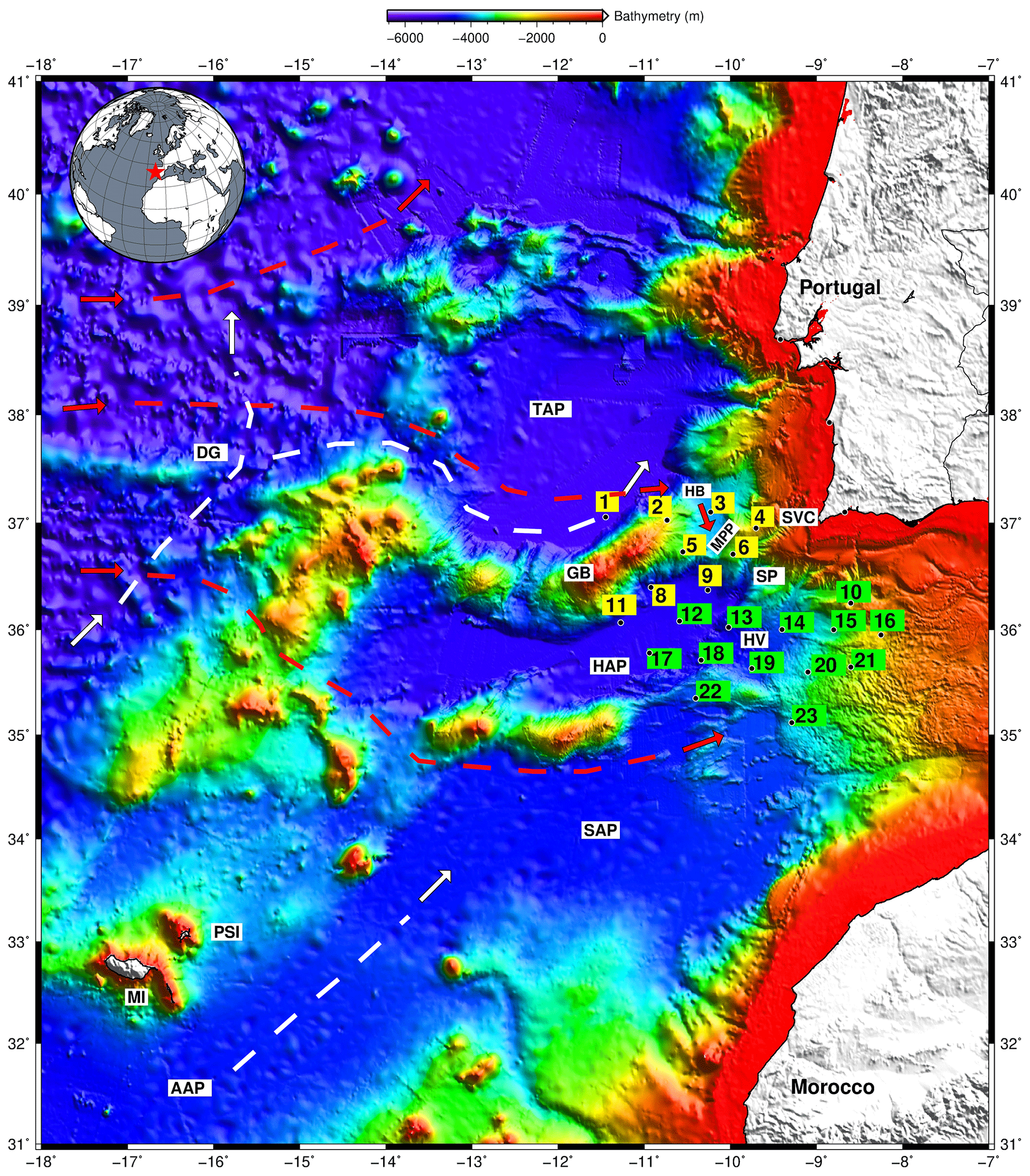
Figure 2LOBSTER OBS location – deployment of OBS (1 represents OBS01, and so on). Main geographical features shown: TAP – Tagus Abyssal Plain; HB – D. Henrique Basin; DG – Discovery Gap; GB – Gorringe Bank; MPP – Marquês de Pombal Plateau; SVC – São Vicente Canyon; SP – Sagres Plateau; HAP – Horseshoe Abyssal Plain; SAP – Seine Abyssal Plain; AAP – Agadir Abyssal Plain; MI – Madeira Island; PSI – Porto Santo Island. The dashed white lines represent the Antarctic Bottom Water (AABW) flowing regionally below 4000 m. The dashed red lines represent the North Atlantic Deep Water (NADW) flowing between 1400–4000 m. We mark the OBSs affected (yellow) or not (green) by the ocean bottom current flow. The OBS 9H OBS01, 9H OBS03 and 9H OBS04 are used in this study.
Voet et al. (2020), working near a tall submarine ridge in the Pacific Ocean, observed the superposition of two distinct energy sources, the tidal and permanent low-frequency flows, with a combined bottom-current speed of 20 cm s−1 in specific periods. Observations showed a stark contrast between conditions at spring and neap tide. The authors concluded that the tide flow speed, in that particular site, during spring tide was higher than the permanent low-frequency flow. Likewise, a minimum tide flow speed was observed through neap tides, and the permanent low-frequency flow dominated over the oscillatory tide flow (Voet et al., 2020). They emphasised that during spring or neap tides, when tide flow was stronger or weaker than the low-frequency flow speed, the resulting current flow was reduced when interacting as opposed to and increased when in phase (Voet et al., 2020). These authors concluded that both tide and low-frequency flows interact with bottom topography. The energy dissipation at any given time is dictated by the total flow speed (sum of tidal and permanent low-frequency flow). The turbulent flow regime observed in the OBSs in SW Iberia may have two contributions: the tidal bottom currents and the permanent low-frequency geostrophic current.
From September 2007 to August 2008, an ocean bottom seismometer experiment, NEAREST Project (Integrated observations from NEAR shore sourcES of Tsunamis: towards an early warning system), took place offshore of Cape S. Vincent and in the Gulf of Cádiz (Geissler et al., 2010), in the Portuguese and Moroccan exclusive economic zones. On board the Italian ship RV Urania, 24 LOBSTER (OBS) from the German instrument pool for amphibian seismology (DEPAS) were deployed at depths ranging from 1990 to 5100 m (Figs. 2 and 3). The FDSN temporary network 9H was assigned during the years 2007 to 2011.

Figure 3LOBSTER OBS – LOBSTER OBS used in NEAREST project. (a) OBS suspended by the ship's crane, waiting for the deploy signal; (b) on the deck of RV Urania ready to be deployed.
The OBSs recorded at a sampling rate of 100 Hz on a three-component Güralp CMG-40TOBS seismometer of 60 s corner period (vertical component Z, horizontal component X and Y; see Fig. 3 for orientation) and on a hydrophone HTI-04/01-PCA. The LOBSTER (Alfred-Wegener-Institut, Helmholtz-Zentrum für Polar- und Meeresforschung et al., 2017) components are illustrated in Fig. 3. The seismometer, hydrophone, data recorder and batteries comprise the acquisition system, while the syntactic foam floats and releaser unit are required only to recover instruments from the seafloor. The flag, radio beacon and flashlight are only needed when OBS surfaces to locate. The head buoy is only used to help retrieve the instrument from the sea surface to the ship. All the elements not required for data recording will also be present on the seafloor facing the current flow connected to the instrument frame. The head buoy floats 7–10 m above the OBS with an 18 mm diameter rope tied to the central OBS mainframe. There are two loops on this rope for retrieval at roughly 3 m intervals. The sub-horizontal flagpole has a diameter of 21 mm and is 1.3 m long. The radio antenna has a diameter of 1.9 mm and is 42 cm long. Both are firmly attached to the OBS frame.
The titanium mainframe has a rigid connection to the gimballed seismometer. According to Stähler et al. (2018), the German pool used the 60 s instrument in a version modified by Güralp for OBS by reducing power consumption and adding a mechanical gimbal system for automated levelling. In addition, the sensor was placed in a titanium casing which caused modifications to the instrument's self-noise. As a result, the self-noise exceeded the new low-noise model (NLNM; Peterson, 1993) for periods of more than 10 s (Tasic and Runovc, 2012).
During this deployment, all the OBS recorded a plethora of signals (e.g. Corela, 2014). This paper will focus on the harmonic tremors (short-period noise band) and tilt noise spectral windows (long-period noise band) triggered by the bottom current flow. In Fig. 2, we mark the OBSs that were affected or almost not by the ocean bottom current flow. Those affected are in yellow, and those that were not are in green (more details in Fig. S20 in the Supplement). This study used the 9H OBS01, 9H OBS03 and 9H OBS04 (see Fig. 4). The influence of deep current flow, tidal and permanent low frequency, is expected to be more pronounced near rougher topography; 9H OBS01 was located at the Tagus Abyssal Plain (TAP), deployed at a depth of 5100 m, within the influence of AABW, and 9H OBS03 in the middle of the D. Henrique Basin at a depth of 3932 m, within the effect of NADW (Fig. 2). Despite the focus, we present information regarding harmonic tremors and tilt noise for all the OBSs. In this work, we also evaluate the harmonic tremor and tilt noise signal recorded on the 9H OBS04 near the São Vicente Canyon (Figs. 2 and 4), at a depth of 1993 m, under the influence of the NADW. This particular OBS was the only one that showed a different harmonic tremors signal that polluted all spectra from 0.5 to 40 Hz, showing a large spectral amplitude.
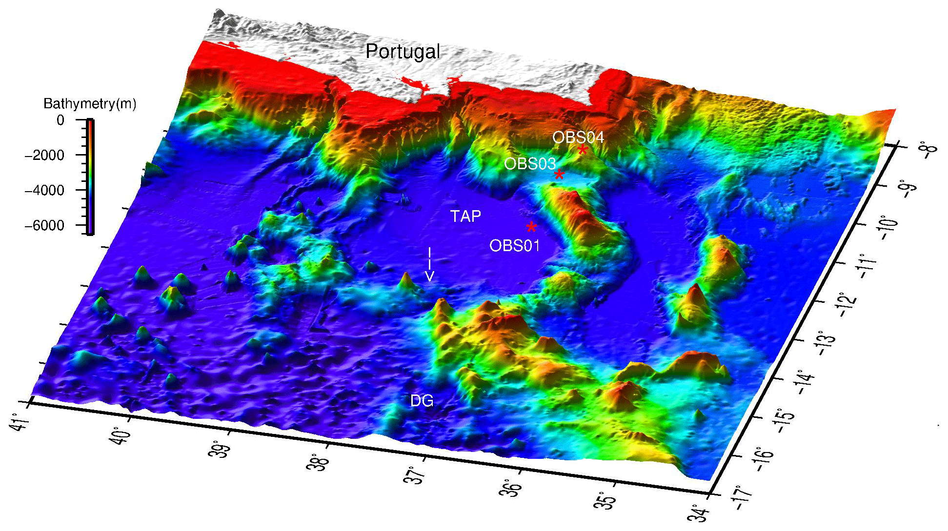
Figure 43D perspectives – location of 9H OBS01, OBS03 and OBS04 in SW Iberia with the local seafloor topography. Portugal is represented as white. The Discovery Gap (DG) is the main gate for the Antarctic Bottom Water (AABW), and the white arrow points out to the main gate where the AABW enters the Tagus Abyssal Plain (TAP).
Based on this characteristic, it was decided to deploy a new broadband OBS developed and built in Portugal at IDL/CEIIA within the DUNE project (PTDC/EAM-OCE/28389/2017) in the seafloor vicinity position of 9H OBS04 to study its behaviour in harsh conditions regarding higher bottom current speed. Accordingly, the DUNE OBS (Fig. 5) was deployed 25 May 2021 and recovered 15 October 2021, primarily associating the environment-generated noise on the two data records despite the long time interval between them.
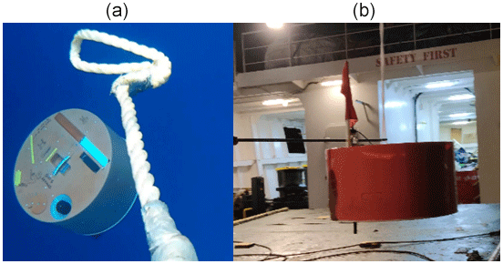
Figure 5DUNE OBS – new broadband OBS developed and built in Portugal with the new seismic sensor Aquarius (120s–100 Hz) from Güralp and a broadband hydrophone HTI-04-PCA. On the left DUNE OBS on free fall in the water column and, on the right, recovery of the DUNE OBS with the flag, radio and flashlight outside the orange shell. The deployment and recovery on board the Portuguese vessel RV Mário Ruivo (IPMA).
The DUNE OBS aimed to mitigate the influence of deep-sea currents on the instrument. The accessories (flag, radio antenna and head buoy) are inside the outer orange shell during the free fall and recording period. After releasing the instrument from the anchor at the seafloor, the flag, radio antenna, flash beacon and head buoy are released from the frame and stand outside the outer shell to simplify its recovery at the surface. For the DUNE campaign, the Güralp Aquarius (120 s–100 Hz) seismometer was firmly connected to the OBS inner structure, similar to the LOBSTER OBS. This sensor is a triaxial orthogonal broadband seismometer operational at ±90∘ with a self-noise of −173 dB re(m s−2)2 Hz−1 at 10 s in the vertical component. The OBS is a cylinder with a diameter of 1 m and a height of 55 cm.
It should be noted that the amplitude of the tilt noise band (20–60 s) and harmonic tremors (0.5–6.5 Hz) are used as a proxy to the bottom flow current speed that impacts the OBS structure. No current meter was used in this work. As a proxy to the tidal forcing of the deep ocean currents, we will use Lagos, Sines and Cascais harbour tide table from 10 to 28 September 2007. This period represents one cycle from spring to neap tide and back to the spring tide (Table S1 in the Supplement). The locations of Lagos, Sines and Cascais tide gauges are given in Fig. 2. The tidal time is almost identical at the different areas separated by hundreds of kilometres (information from Hydrographic Institute, https://www.hidrografico.pt/prev.mare, last access: 12 April 2023). It should be noted that the tidal range away from the coast is lower than the nearby coast.
We concentrate the OBS-recorded noise analysis on two frequency bands, the short-period (harmonic tremors) and the long-period (tilt noise) bands, in the seismometer's horizontal Y and vertical Z components. As a result, we expected to see a robust seismometer response during the spring tide by deep ocean currents modulated by the tide and during the neap tides, a significant impact from the permanent low-frequency flow, AABW and NADW.
4.1 Deep ocean current regime as inferred from OBS noise
The spectrograms of 9H OBS01 and 9H OBS03 during the new moon spring tide are seen in Fig. 6 for the horizontal components HHY (vertical components HHZ, in Fig. S2). At the spring tide of 11 September 2007, the tide current flow speed, during the flood and ebb tide, should give higher amplitude in spectrograms in the harmonic tremor and tilt noise band when impacting the OBS structure. The tidal range, the high tide amplitude minus the low tide amplitude, is 2.9, 2.8 and 2.8 m, measured in Lagos, Sines and Cascais tide gauge, respectively. The 9H OBS01, located at TAP, reveals a higher current flow speed during the flood tide, reaching a maximum amplitude of −80 dB in the tilt noise band and a maximum amplitude of −90 dB in the harmonic tremor band. During the ebb tide, the tilt noise amplitude on the spectrogram decreases to −110 dB, and the harmonic tremors are not triggered. The 9H OBS03 shows a different response. During the ebb tide, the resulting current flow speed tilts the seismometer amplitude to −89 dB and the harmonic tremor to −100 dB. During the flood tide, the maximum tilt noise amplitude decreases to −110 dB, and the harmonic tremors are not triggered.

Figure 6Spring tide at new moon – spectrograms of 9H OBS01 and 9H OBS03 (11 September 2007) during the spring tide. The OBS shows different responses to the tide and low-frequency current flows. During the spring tide the tidal range in Sines was 2.8 m.
During the first quarter moon, the neap tide of 20 September 2007 (Fig. 7), the tidal range measured in Lagos, Sines and Cascais was 0.7, 0.7 and 0.7 m, respectively, and the tide current flow speed reached a minimum. For 9H OBS01, the permanent low-frequency flow dominates over the tide oscillatory flow, with a tilt noise amplitude of −100 dB, increasing to −90 dB during the flood tide. As a result, the harmonic tremors reach a maximum amplitude of −100 dB during the flood tide. In the same period, 9H OBS03 shows a low-frequency flow domination with an amplitude between −110 and −100 dB in the tilt noise band, and the harmonic tremors are not visible.
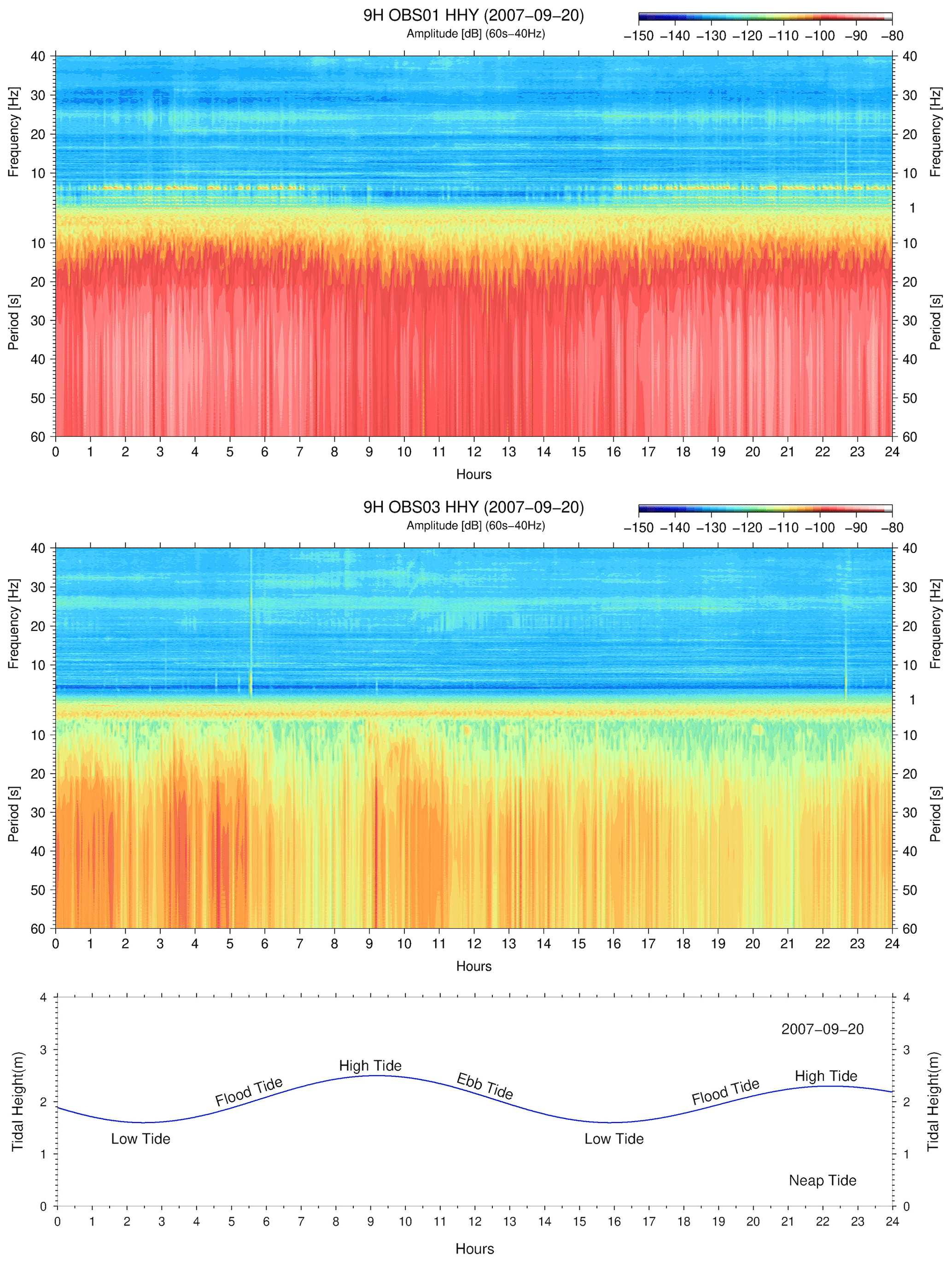
Figure 7Neap tide in quarter moon – 9H OBS01 and 9H OBS03 spectrograms during the neap tide period (20 September 2007). The permanent low-frequency flow dominates over the tide flow. The tidal range in neap tide was 0.7 m (measured in Sines).
After the full moon (26 September 2007), the spring tide has a tidal range of 3.5, 3.5 and 3.6 m, measured at Lagos, Sines and Cascais, respectively (28 September 2007, Fig. 8). The tide current flow speed reaches again to a maximum. The 9H OBS01 impact is higher during the flood tide with a maximum amplitude of −80 dB in the tilt noise band and a maximum amplitude of −89 dB in the harmonic tremors. During the influence of the ebb tide, the tilt noise amplitude decreases to −105 dB with no visible harmonic tremor. Similar spectrograms are observed during both spring tides (11 and 28 September 2007). On 9H OBS03, at the D. Henrique Basin, the current flow speed is higher during the ebb tide, attains an amplitude of −100 dB in the tilt noise band, and the harmonic tremors are not triggered. See supplementary figures S2 to S19 to infer the amplitude of the horizontal Y and vertical Z spectrograms in the tilt noise band and the harmonic tremors from 10 to 28 September 2007.
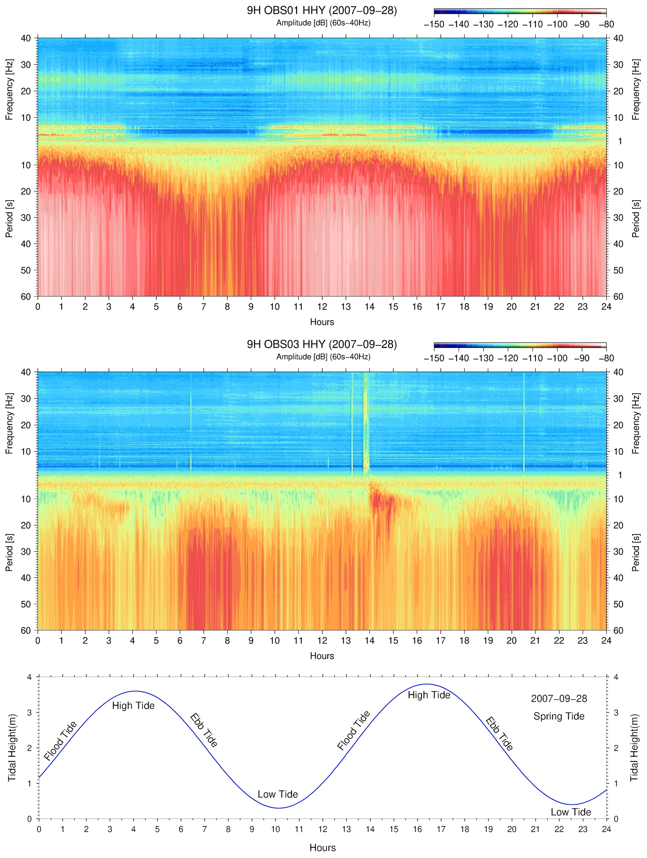
Figure 8Spring tide at full moon – 9H OBS01 and 9H OBS03 spectrograms during the spring tide (28 September 2007). The OBSs respond differently to the energy balance between the tide and the permanent low-frequency flows. The 9H OBS01 during flood tide and 9H OBS03 in ebb tide. During the spring tide, the tidal range was 3.5 m (measured in Sines).
The recorded amplitude on the spectrograms increases, in the long-period (tilt noise) and short-period (harmonic tremors) bands, when the laminar flow that impacts the OBS becomes a turbulent flow due to an increase in the current flow speed. This boundary we call the current flow speed threshold, which is different for the diverse OBS resonance components, like the floating units, several titanium tubes, rope, flagpole and radio antenna.
4.2 Harmonic tremor structure
Zooming in on the harmonic tremor, as an example, on 11 September, it is possible to observe, during the flood tide, that the OBS components which have the resonant frequency inside the short-period noise domain starts to resonate (Fig. 9, 9H OBS01 HHZ). That is the case of the resonance of the head buoy rope, flagpole, radio antenna and the OBS–sediment coupling. The head buoy rope is tied directly to the OBS's titanium tubing mainframe and held taut by the syntactic foam float. The flagpole and radio antenna have a rigid connection with the titanium frame. With a gimbal system, the seismic sensor has a firm connection to the titanium mainframe and is pressed against the anchor (see Fig. 3).

Figure 9Harmonic tremors – the prevailing signals before, during and after the harmonic tremors. The current flow speed described in terms of (A) radio antenna, (F) flagpole, (R1) head buoy rope fundamental frequency, (R2) second, (R3) third, (R4) and fourth overtones, and (C) the natural frequency of OBS–sediment coupling. At (1) 07:30, before the harmonic tremors, with its normal vibration; (2) 09:40, observed frequency gliding in the head buoy rope; (3) 10:50, we observe mode-locking frequency on harmonic tremor; (4) 13:10, continues the previous situation in terms of frequency (mode-locking); (5) 15:30, the current flow speed is decreasing and a frequency gliding of the head buoy rope is observed; (6) 18:00, the harmonic tremor is no longer active and the natural frequency of OBS–sediment coupling returns to normal.
From the spectrogram, which highlights the harmonic tremors, the first emergent resonance is due to the head buoy rope fundamental frequency (R1), afterwards the rope overtones (R2, R3, R4), radio antenna (A) and finally the flagpole (F) eigenvibrations. Before and after the harmonic tremors (Fig. 9, (1) and (6)), the dominant signal is the natural frequency of OBS–sediment coupling resonance (C), between 5.5 and 5.7 Hz, observed during the entire recording period of the campaign. This signal is easily detected on the upper spectrogram from 7 to 9 h and from 16 to 19 h.
The head buoy rope fundamental frequency (R1) starts to vibrate around 09:05 (Fig. 9). The current flow causes the tensioned cable to strum (Stähler et al., 2018). At 09:15, the head buoy rope overtones (R2, R3, R4) emerge at integer multiples of the fundamental frequency. During this period, the von Kármán vortex shedding off the rope is at a frequency lower than the resonance frequency of the rope and is observed in the frequency-gliding phenomena. At the same time, the radio antenna (A) starts to resonate, and a minor frequency gliding is observed. At 09:40, four signals from the head buoy rope are visible, during frequency gliding, with 0.92, 1.84, 2.76 and 3.68 Hz. The OBS–sediment coupling (C) is amplified at this time with a frequency of around 5.7 Hz. The current flow speed at 10:00 initiated a new effect called a wake or lock-in (Skop and Griffin, 1975; Griffin, 1985, and described by Stähler et al., 2018), denominated mode-locking frequency, stable until 14:00, which is boosted when vortex shedding frequency is equal or close to the resonant frequency of the rope, radio antenna and flagpole. At 10:30, the flagpole (F) eigenvibrations begin, without any frequency gliding, and keep the signal until 13:30. Between (3) 10:50 and (4) 13:10 (Fig. 9), for example, it is possible to identify the flagpole signal (F) with 1.45 Hz, radio antenna (A) at 6.4 Hz and the fundamental and overtones of the head buoy rope (R1 around 1.17 Hz, R2 near 2.34 Hz, R3 at 3.51 Hz and R4 around 4.68 Hz). At (5) 15:30, R1, R2, R3 and R4 have a noticeable decrease in amplitude and frequency due to the reduction of current flow speed. Around (6) 18:00, the OBS returns to its natural state, and the observed signal is the natural frequency of the OBS–sediment coupling resonance (C). In the short (harmonic tremors), the recorded amplitude on the spectrograms increases when the laminar flow that impacts the OBS becomes a turbulent flow due to an increase in the current flow speed. The current flow speed threshold differs for the short-period OBS components that resonate.
4.3 Noise levels observed on 9H OBS04 and LX OBS01
During the NEAREST campaign in 2007, 24 OBSs were deployed and analysed. Most of the OBSs were deployed in areas where the current flow speed was not enough to trigger the harmonic tremors (Corela, 2014). However, 9H OBS04 (see Figs. 2 and 4) was deployed in an area where when the current flow speed impacts the OBS structure, it gives rise to a different OBS response not observed on other LOBSTER OBSs in the short and long-period band noise. The harmonic tremors and tilt noise showed a larger spectral amplitude (−60 dB) when compared with 9H OBS01 and 9H OBS03 (maximum spectral amplitude of −83 dB). The mode-locking is not always present. This response was observed, as an example, most of the day of 14 October 2007 (Fig. 10).
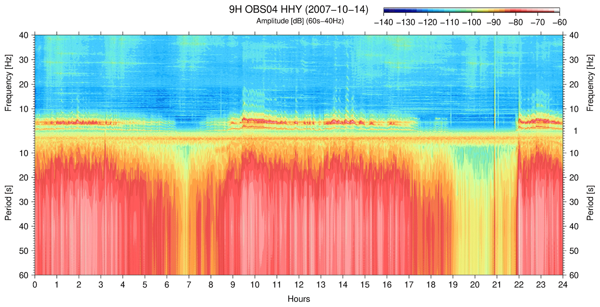
Figure 10Strong harmonic tremor – the effect of strong current flow speed when impacts the head buoy rope between 1–40 Hz.
The LX OBS01 was deployed at the exact sea surface location as 9H OBS04 to study the response of the OBS in an environment where a strong current flow speed is expected, as noted in previous studies. Searching for periods of solid tilt noise and associated noise in the first short-period domain, for instance, during 20 September 2021 (Fig. 11), the harmonic tremors were not triggered because the radio antenna, flagpole and head buoy rope were isolated from vibrations and safely stowed inside the OBS shell (see Fig. 5). However, the natural frequency OBS–sediment coupling was observed as expected because the seismometer is connected firmly to the OBS structure. During the strong current flow speed scenario, the OBS vibrates when impacted by the current flow.
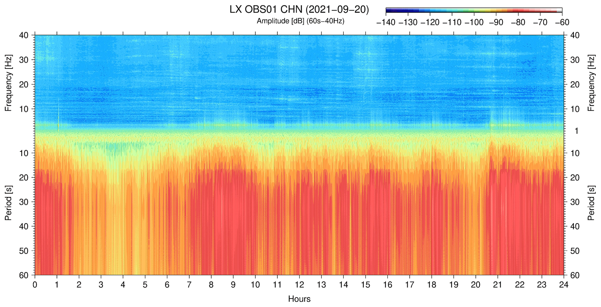
Figure 11LX OBS01 spectrogram – on this particular day, a strong current flow scenario was observed during the campaign without harmonic tremors with noise around the natural frequency of OBS–sediment coupling resonance. The tilt noise, resulting from the current flow impact on the OBS structure, was observed almost during the entire day.
We processed data on all OBS available during the period of this study. In Fig. 2, we mark the OBSs that recorded tilt noise and harmonic tremors due to ocean bottom currents in yellow and those that did not appear in green (see also Fig. S20) during the time interval analysed in this study. As expected, seafloor topography irregularities have an enormous responsibility in adjusting the speed flow field. Therefore, we chose the OBSs, 9H OBS01 and 9H OBS03 because they were installed at locations where the bottom current speed effect is evident. The tidal bottom current and the permanent low-frequency currents, AABW and NADW, are evident in these two spots.
The AABW, flowing below 4000 m, needs oceanic gateways to move into the abyssal plains (Hernández-Molina et al., 2011). The Discovery Gap (DG in Fig. 2) is an essential gateway for deep water circulation in Tagus Abyssal Plain. Figure 2 shows that AABW, a dashed white line near 9H OBS01, 5100 m deep at TAP, moves from SW to NE. The bottom tidal current, aligned along the bathymetric contour, the flood tide describes a movement from SW to NE and the ebb tide on the contrary direction. The permanent low-frequency AABW current is in phase with the flood tide, and the total flow speed is the sum of the two contributions. This flow speed, during the spring tide of 11 September 2011 (new moon, Fig. 6, 9H OBS01 HHY), gives −83 dB (maximum amplitude) in the tilt noise and −90 dB in the harmonic tremors. During the spring tide of 28 September 2007 (full moon, Fig. 8, 9H OBS01 HHY), −80 dB in the tilt noise and −87 dB in the harmonic tremors. During the ebb tide, the tidal and the permanent low-frequency AABW currents are in opposing directions, and the total flow speed decreases. As a result, the current flow speed in the tilt noise band decrease to a maximum amplitude of −110 dB and the harmonic tremors' resonances cease their movement. In both spring tides, the behaviour of the 9H OBS01 is identical. During neap tide, 20 September 2007 (first quarter moon, Fig. 7, 9H OBS01 HHY), the permanent low-frequency AABW is noticeable all day with a constant recorded amplitude of −100 dB and, during the period of the flood tide, increases to −90 dB. In these two flood tide periods, the little increase in current flow speed is sufficient for the harmonic tremors resonances to appear with a maximum amplitude of −100 dB.
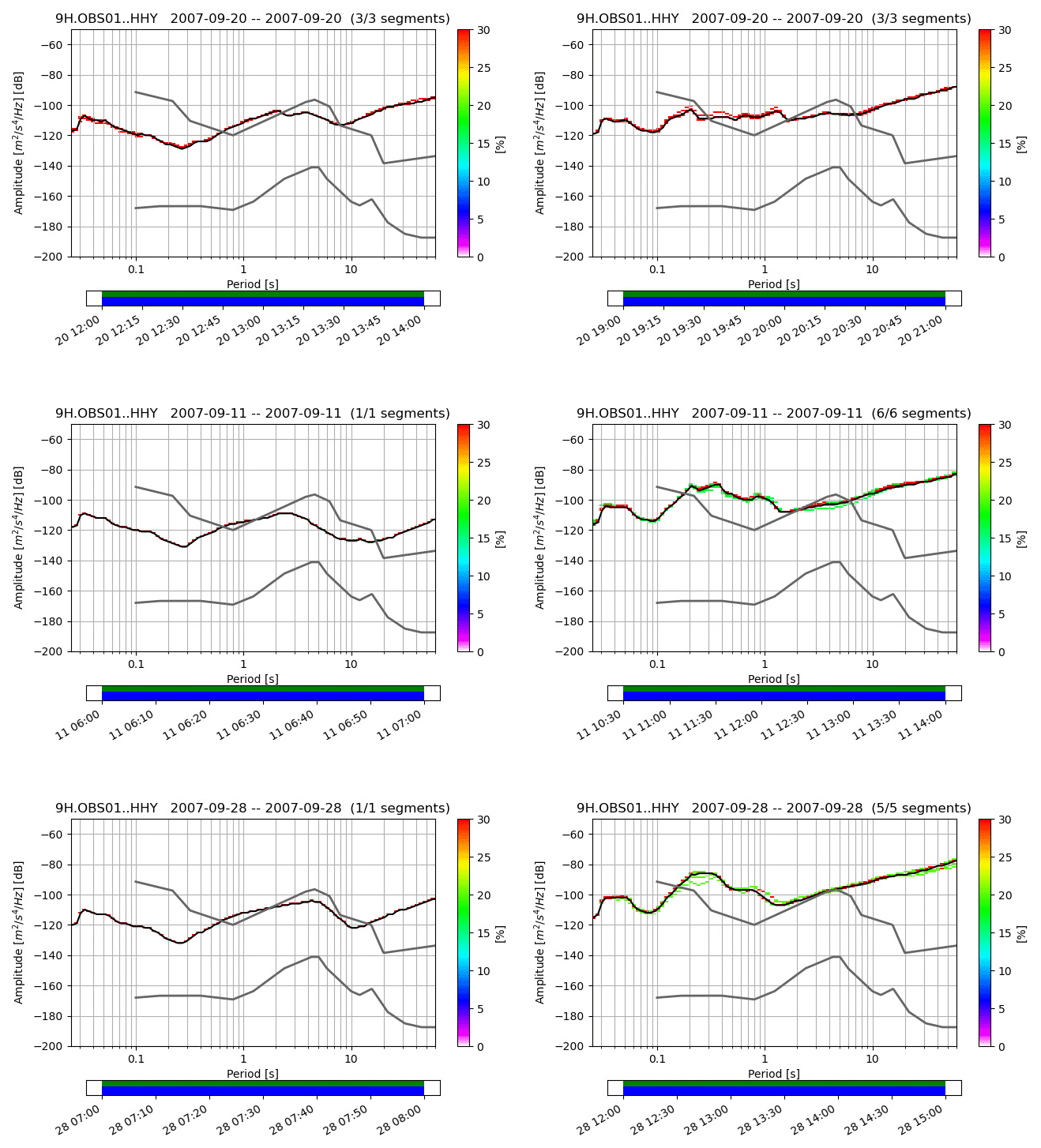
Figure 12PPSD of 9H OBS01 for the spring and neap tides – on top, PPSD for the 20 September 2007 (first quarter moon neap tide with 0.7 m tidal range), middle at 11 September 2007 (new moon spring tide with 2.8 m tidal range) and on the bottom the 27 September 2007 (full moon spring tide with 3.5 m tidal range). On the left, the seismometer response during laminar flow and, on the right, during turbulent flow.
Figure 12 shows the probabilistic power spectral densities (PPSDs), from 9H OBS01 Güralp CMG-40TOBS, during the neap and spring tides. It is possible to infer the response of the seismometer during the laminar flow (Fig. 12, left side) and the turbulent flow (Fig. 12, right side). During the neap tide, with laminar flow between 12 and 14 h, within the ebb tide of 20 September 2007, the response, between 3–40 Hz, was inside the Peterson noise curves and exceeded the new low-noise model for periods higher than 1 s. Within the turbulent flow (Fig. 12, right side, flood tide, 20 September 2007, between 19 and 21 h, 0.7 m tidal range in Sines), as an example, for 30 s, from the laminar to turbulent flow, the tilt noise band increases from −100 to −93 dB (7 dB) and in harmonic tremor band, at 5 Hz, from −125 to −102 dB (23 dB). During 11 September 2007 (2.7 m tidal range in Sines), laminar to turbulent flow increased from −120 to −87 dB in the tilt noise band (37 dB) and harmonic tremor band, 5 Hz, from −127 to −90 dB (37 dB). On 28 September 2007 (3.5 m tidal range in Sines), laminar to turbulent flow increased from −110 to −82 dB in the tilt noise band (28 dB) and in the harmonic tremor band from −130 to −85 dB (45 dB). The impact of current flow outcomes a seismometer higher spectral amplitude in the short-period band.
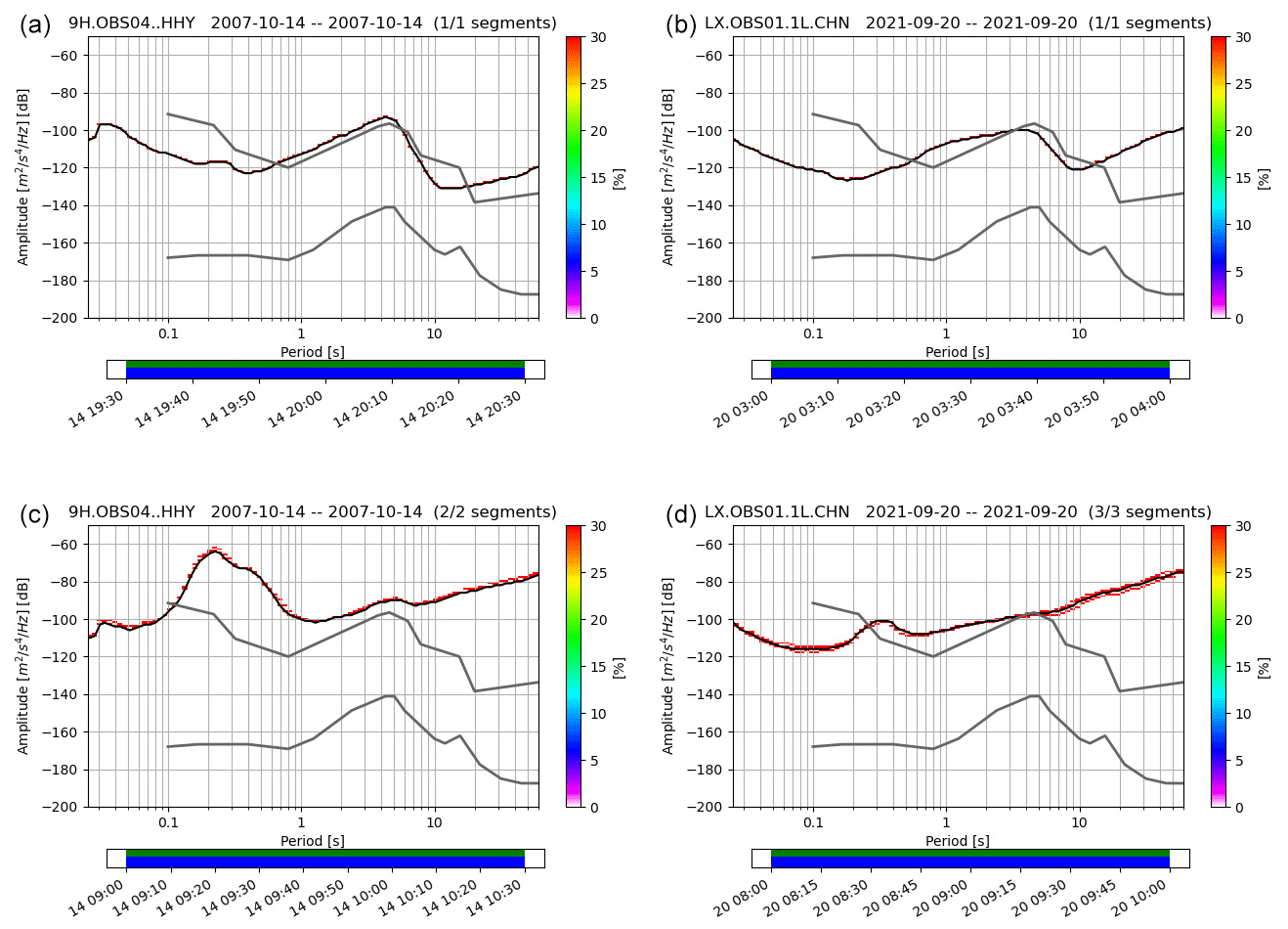
Figure 13PPSD of 9H OBS04 and LX OBS01 during laminar and turbulent flow events – different high current flow speed scenarios on 14 October 2007 (9H OBS04) and 20 September 2021 (LX OBS01). The upper part of the figure represents the laminar flow scenario in both OBSs, and the bottom part is the turbulent one.
In the 9H OBS03, D. Henrique Basin area, the tide bottom current and the permanent low-frequency current, NADW, cause tilt noise and harmonic tremors. In this basin, the tide bottom current still describes an elliptical hodograph in the anticlockwise direction parallel to the coast. The flood tide is from south to north, and the ebb tide is in the opposite direction. The permanent low-frequency current, NADW (dashed red line, Fig. 2), shows a trend from NNW to SSE. The permanent low-frequency NADW is almost in phase with the ebb tide and nearly opposite to the flood tide. During the spring tide, 11 September 2007 (Fig. 6, 9H OBS03 HHY), the maximum amplitude recorded in the tilt noise occurred only during the two periods of the ebb tide, −90 dB. Only during these ebb tide periods is the current flow speed threshold attained, and the harmonic tremors rise with a maximum amplitude of −100 dB. During the spring tide of 28 September 2007 (Fig. 7, 9H OBS03 HHY), surprisingly, the maximum amplitude recorded in the tilt noise band was −100 dB during the two periods of the ebb tide. Nevertheless, the current flow speed threshold is not attained, and the harmonic tremors are not triggered. One possible explanation is a decreased current flow speed in the permanent low-frequency NADW. This explanation is corroborated by the spectrogram recorded during the neap tide of 20 September (Fig. 7, 9H OBS03 HHY), where we see an intermittent flow of the permanent low-frequency NADW current. Consulting the supplement figures, from Figs. S2 to S19, a speed decrease of permanent low-frequency NADW current flow between 13 and 14 of September 2007 shows two ebb tides and two flood tides. After the 23 of September 2007, the permanent low-frequency NADW current flow increases the speed, in phase again with the ebb tide. However, the total flow speed is less than the current flow speed threshold necessary to initiate the harmonic tremors. From 11 to 28 September 2007, the permanent low-frequency flow observed in TAP, the AABW current, shows an intense and persistent direction. In contrast, the NADW current is intermittent and has a lower speed flow when compared to the AABW.
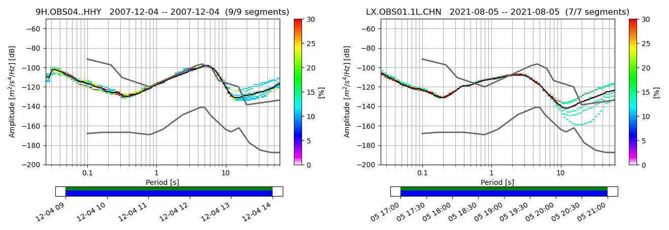
Figure 14Response – the response of CMG-40T and Aquarius seismometer, both from Güralp, to laminar flow. The Güralp CMG-40T (9H OBS04) has a standard response between 10 s–40 Hz and exceeds the new low noise model for periods above 10 s. The Güralp Aquarius (LX OBS01) shows −160 dB re((m s−2)2 Hz−1) between 15 and 20 s.
We show that the ocean bottom flow, as inferred from the tilt noise, is not an exclusive function of the tidal forcing. Instead, it is shown that the ocean bottom has a flow regime that may have two contributions – the permanent low-frequency current and the tidal current – as mentioned in Voet et al. (2020). The recorded tilt noise displays the balance between these two currents along the entire tidal cycle, between neap and spring tides. From these current flows, it is possible to highlight that the most relevant parameter to the OBS noise recorded is the resulting current flow speed due to both currents or just one of them. For example, in Fig. 1, during the neap tide of 19 October 2007, with a tidal range of 0.8 m (measured in Sines), it was possible to observe harmonic tremors features for as long as 24 h in 9H OBS01. The permanent low-frequency flow triggered the resonance state, but a tidal modulation can still be inferred.
Highlighting the harmonic tremor spectral band, the 9H OBS01 components with a resonant frequency inside the short-period noise domain start to resonate during the flood tide. When the current flow speed threshold is reached and exceeded, and when we observe the frequency mode-locking, the vortex shedding frequency is equal to or close to the resonant frequency of the several components of the OBS. This allows us to infer the current flow speed observed in this particular location in harmonic tremors. For example, in Fig. 9 (4), at 13:10 on 11 September 2007, the observed resonance frequency of the radio antenna is 6.4 Hz and for the flagpole is 1.45 Hz. The shedding frequency is proportional to the Strouhal number, which for this OBS design is 0.21, and to the current flow speed, in centimetres per second, and inversely proportional to the diameter of the OBS component (see, e.g. Stähler et al., 2018). One of the first components to enter a resonant state is the radio antenna (diameter of 0.19 cm), which only needs a current flow speed of 5.3 to 5.5 cm s−1 to reach the frequency mode-locking. For the flagpole, with a diameter of 2.1 cm, the current flow speed must equal 15 cm s−1. Applying this reasoning to the spectrum of Fig. 9, we infer that between 10:10 and 10:30, the current flow speed is limited to the range of 5 to 15 cm s−1, between 10:30 and 13:30 at least equal to or higher than 15 cm s−1, between 13:30 and 14:10 to the range of 15 to 5 cm s−1, and between 14:20 and 15:40 below 5 cm s−1. The maximum harmonic tremor spectral amplitude observed in 9H OBS01 was −85 dB (Fig. 12). From Fig. 13, 9H OBS04, with a maximum harmonic tremor spectral amplitude of −63 dB, one possible conclusion is that the current flow speed can reach 50 cm s−1 or more, as proposed by Hernández-Molina et al. (2011).
Due to the large spectral amplitude detected near São Vicente Canyon, owing to the high current flow speed observed in this region, we showed the noise levels of 9H OBS04 and LX OBS01 (Fig. 13). Two windows, one with laminar flow and one with turbulent flow, as identified in Figs. 10 and 11, were chosen to illustrate the seismometer response when impacted by the current flow. For 9H OBS04, an increase of the spectral amplitude of 47 dB at the tilt noise band (30 s) was observed and an increase of 56 dB in the short-period band (5 Hz). For the LX OBS01, we observed a gain of 23 dB at the tilt noise band (30 s), and we observed an increase of 23 dB in the short-period band (one spectral line of 3.8 Hz, which is the natural frequency of the OBS–sediment coupling resonance). When both stations were impacted by laminar flow (Fig. 13), the natural response of the seismometers at the sea bottom was recorded. The Güralp CMG-40T has a standard response between 10 s–40 Hz and exceeds the new low-noise model for periods above 10 s. On the other hand, the Güralp Aquarius shows −160 dB re(m s−2)2 Hz−1 between 15 and 20 s (Fig. 14). However, in the turbulent regime, we can infer that better performance of the LX OBS is only attained for lower periods.
This new design, DUNE OBS, is still highly exposed to the current flow. Therefore, later iterations are aimed, at the long-period noise band, since the tilt noise still needs to be mitigated. Research into solving this problem is already in progress, and further work needs to be carried out to establish improvements in OBS design. Future work should focus on changing the seismic sensor position and disconnection from the OBS structure in a smaller package. This action should shift the natural frequency of the OBS–sediment coupling resonance to above the seismologically interested frequency band and mitigate the tilt noise. Similar design changes could also improve the signal of the LOBSTER OBS.
This study finds that the harmonic tremors and the tilt noise signal are independent of the current direction relative to the OBSs in both designs. The features are in all seismometer components (Fig. S21). However, the difference in the spectral amplitude of the signal on the horizontal components could give some insight into the path of the current flow field.
Analysing seismic data recorded by OBS in the SW Iberia, we showed that the short-period (0.5–6.5 Hz) and long-period (20–60 s) noise bands have an environmental origin of deep ocean currents. However, each site is unique regarding depth, currents and seafloor topography. Furthermore, this work shows that tidal forcing does not always dominate the ocean bottom flow, as inferred from the tilt noise. Instead, the ocean bottom has a flow regime that may have two independent contributions: the permanent low-frequency current and the tidal current. The recorded noise displays the balance between these two currents along the entire tidal cycle, between neap and spring tides, and depends on the direction of each flow and the final combined current flow speed.
In the short-period noise domain, we investigated the harmonic tremor band (0.5–6.5 Hz) in detail. We showed that all the mechanical elements of the OBS that are not essential for recording at sea bottom do resonate when the current speed reaches some threshold. Noise is shown on spectrograms by nearly constant frequency bands and broadband spectral lines.
These findings support the interpretation that the strongest harmonic tremors are the result of the strumming of the head-buoy rope on the LOBSTER design (Stähler et al., 2018; Essing et al., 2021) and confirmed that the radio antenna, flagpole and the natural frequency of OBS–sediment coupling resonance are also excited by the current flow speed when the laminar flow became turbulent in each component. The head buoy rope's fundamental frequency and respective overtones exhibit frequency gliding. These characteristics are reported in different studies. However, the strumming rope frequencies reported in this study differ from those reported previously (e.g. Stähler et al., 2018; Essing et al., 2021). The radio antenna exhibits a smaller amplitude, and the flagpole has no visible frequency gliding. When the frequency of vortex shedding is near or identical to the resonance frequency of the different components, we observe the mode-locking frequency, which gives some insight into the minimum current flow speed threshold that causes that disturbance.
Our study provides evidence for another noise regime without precise mode-locking frequency when a robust current flow triggers the several resonance components of the OBS. In 9H OBS04, the observed harmonic tremor starts with frequency gliding, but the mode-locking frequency state is attained only on several occasions. The observed harmonic tremor increased the spectral amplitude and enlarged the number of overtones.
Code used in this research can be obtained from the first author upon reasonable request.
The resulting data can be obtained from the first author upon reasonable request. The LOBSTER OBS data, acquired in SW Iberia, near Portugal, are a contribution of project NEAREST FP6-2005-GLOBAL-4 (OJ 2005C177/15). The new broadband OBS data were provided by the DUNE project (PTDC/EAM-OCE/28389/2017, https://idl.ciencias.ulisboa.pt/dune-project, last access: 17 April 2023; Instituto Dom Luiz, 2023) and the EMSO-PT project (PINFRA/22157/2016, https://emso-pt.pt/, last access: 17 April 2023; EMSO Portugal, 2020).
The supplement related to this article is available online at: https://doi.org/10.5194/nhess-23-1433-2023-supplement.
All authors prepared the manuscript and jointly reviewed and edited subsequent drafts.
The contact author has declared that none of the authors has any competing interests.
Publisher’s note: Copernicus Publications remains neutral with regard to jurisdictional claims in published maps and institutional affiliations.
Instruments were provided by Deutscher Geräte-Pool für Amphibische Seismologie (DEPAS) at Alfred Wegener Institute Bremerhaven and Deutsches GeoForschungsZentrum Potsdam (https://doi.org/10.17815/jlsrf-3-165). The authors are grateful to Instituto Dom Luiz (IDL), Faculdade de Ciências da Universidade de Lisboa (FCUL), Instituto Português do Mar e da Atmosfera (IPMA) and CEIIA. The authors are also grateful to the crew of RV Mário Ruivo for the excellent support during the deployment and retrieval of OBSs. Finally, we acknowledge the contributions of the reviewers Wolfram Geissler and one anonymous referee and the editor, Rachid Omira, whose thoughtful feedback improved the quality of this article. Figures for this article and to the Supplement were created using Generic Mapping Tools (GMTs) (Wessel et al., 2013) and ObsPy (Krischer et al., 2015).
This work was funded by Portuguese Fundação para a Ciência e a Tecnologia (FCT) I.P./MCTES through national funds (PIDDAC) – UIDB/50019/2020 – Instituto Dom Luiz (IDL).
This paper was edited by Rachid Omira and reviewed by Wolfram Geissler and one anonymous referee.
Alfred-Wegener-Institut, Helmholtz-Zentrum fur Polar- und Meeresforschung: DEPAS (Deutscher Gerate-Pool fur amphibische Seismologie): German Instrument Pool for Amphibian Seismology, J. Largescale Res. Facil., 3, A122, https://doi.org/10.17815/jlsrf-3-165, 2017.
Almeida, M. M. and Dubert, J.: The structure of tides in the Western Iberia region, Cont. Shelf Res., 26, 385–400, https://doi.org/10.1016/j.csr.2005.11.011, 2006.
An, C., Cai, C., Zhou, L., and Yang, T.: Characteristics of low-frequency horizontal noise of ocean-Bottom Seismic data, Seismol. Res. Lett., 93, 257–267, https://doi.org/10.1785/0220200349, 2022.
Ardhuin, F., Gualtieri, L., and Stutzmann, E.: How ocean waves rock the Earth: Two mechanisms explain microseisms with periods 3 to 300 s, Geophys. Res. Lett. 42, 765–772, https://doi.org/10.1002/2014GL062782, 2015.
Bazin, S., Feuillet, N., Duclos, C., Crawford, W., Nercessian, A., Bengoubou-Valérius, M., Beauducel, F., and Singh, S. C.: The 2004–2005 Les Saintes (French West Indies) seismic aftershock sequence observed with ocean bottom seismometers, Tectonophysics, 489, 91–103, https://doi.org/10.1016/j.tecto.2010.04.005, 2010.
Bowden, D. C., Kohler, M. D., Tsai, V. S., and Weeraratne, D. S.: Offshore Southern California lithospheric velocity structure from noise cross-correlation functions, J. Geophys. Res.-Solid Earth, 121, 3415–3427, https://doi.org/10.1002/2016JB012919, 2016.
Bromirski, P. D., Duennebier, F. K., and Stephen, R. A.: Midocean microseisms, Geochem. Geophys. Geosys., 6, Q04009, https://doi.org/10.1029/2004GC000768, 2005.
Civiero, C., Strak, V., Custódio, S., Silveira, G., Rawlinson, N., Arroucau, P., and Corela, C.: A common deep source for upper-mantle upwellings below the Ibero-western Maghreb region from teleseismic P-wave travel-time tomography, J. Geophys. Res.-Solid Earth, 124, 1781–1801, https://doi.org/10.1029/2018JB016531, 2018.
Civiero, C., Custódio, S., Rawlinson, N., Strak, V., Silveira, G., Arroucau, P., and Corela, C.: Thermal nature of mantle upwellings below the Ibero-western Maghreb region inferred from teleseismic tomography, Earth Planet. Sci. Lett., 499, 157–172, https://doi.org/10.1016/j.epsl.2018.07.024, 2019.
Corela, C.: Ocean bottom seismic noise: applications for the crust knowledge, interaction ocean-atmosphere and instrumental behavior, PhD thesis – Science Faculty of Lisbon University, 1-353, http://hdl.handle.net/10451/15805 (last access: 12 April 2023), 2014.
Corela, C., Silveira, G., Matias, L., Schimmel, M., and Geissler, W.: Ambient seismic noise tomography of SW Iberia integrating seafloor and land-based data, Tectonophysics, 700–701, 131–149, https://doi.org/10.1016/j.tecto.2017.02.012, 2017.
Crawford, W. C. and Webb, S. C.: Identifying and removing tilt noise from low-frequency (< 0.1 Hz) seafloor vertical seismic data, B. Seismol. Soc. Am., 90, 952–963, https://doi.org/10.1785/0119990121, 2000.
Díaz, J., Gallart, J., and Gaspà, O.: Atypical seismic signals at the Galicia Margin, North Atlantic Ocean, related to the resonance of subsurface fluid-filled cracks, Tectonophysics, 433, 1–13, https://doi.org/10.1016/j.tecto.2007.01.004, 2007.
Doran, A. K. and Laske, G.: Infragravity waves and horizontal seafloor compliance, J. Geophys. Res., 121, 260–278, https://doi.org/10.1002/2015jB012511, 2015.
Duennebier, F. K. and Sutton, G. H.: Fidelity of ocean bottom seismometers, Mar. Geophys. Res., 17, 535–555, https://doi.org/10.1007/BF01204343, 1995.
Duennebier, F. K., Blackinton, J. G., and Sutton, G.: Current-Generated Noise Recorded on Ocean Bottom Seismometers, Mar. Geophys. Res., 5, 109–115, https://doi.org/10.1007/BF00310316, 1981.
EMSO Portugal: Monitorização continuada de fatores bióticos e abióticos através de observatórios submarinos, https://emso-pt.pt/ (last acccess: 17 April 2023), 2020.
Essing, D., Schlindwein, V., Schmidt-Aursch, M. C., Hadziioannou, C., and Stähler, S. C.: Characteristics of Current-Induced Harmonic Tremor Signals in Ocean-Bottom Seismometer Records, Seismol. Res. Lett., 92, 3100–3112, https://doi.org/10.1785/0220200397, 2021.
Franek, P., Mienert, J., Buenz, B., and Géli, L.: Character of seismic motion at a location of a gas hydrate bearing mud volcano on the SW Barents Sea margin, J. Geophys. Res., 119, 6159–6177, https://doi.org/10.1002/2014JB010990, 2014.
Garrett, C. and Kunze, E.: Internal Tide Generation in the Deep Ocean, Ann. Rev. Fluid Mech., 39, 57–87, https://doi.org/10.1146/annurev.fluid.39.050905.110227, 2007.
Geissler, W. H., Matias, L., Stich, D., Carrilho, F., Jokat, W., Monna, S., IbenBrahim, A., Mancilla, F., Gutscher, M.-A., Sallarès, V., and Zitellini, N.: Focal mechanisms for sub–crustal earthquakes in the Gulf of Cadiz from a dense OBS deployment, Geophys. Res. Lett., 37, L18309, https://doi.org/10.1029/2010GL044289, 2010.
Griffin, O. M.: Vortex-induced vibrations of marine cables and structures, Technical Report, Naval Research Lab, Washington, D. C., https://apps.dtic.mil/dtic/tr/fulltext/u2/a157481.pdf (last access: 12 April 2023), 1985.
Hernández-Molina, F. J., Serra, N., Stow, D. A. V., Llave, E., Ercilla, G., and van Rooij, D.: Along-slope oceanographic processes and sedimentary products around the Iberian margin, Geo-Mar. Lett., 31, 315–341, https://doi.org/10.1007/s00367-011-0242-2, 2011.
Hernández-Molina, F. J., Wåhlin, A., Bruno, M., Ercilla, G., Llave, E., Serra, N., Rosón, G., Puig, P., Rebesco, M., Van Rooij, D., Roque, D., González-Pola, C., Sánchez, F., Gómez, M., Preu, B., Schwenk, T., Hanebuth, T. J. J., Sánchez Leal, R. F., García-Lafuente, J., Brackenridge, R. E., Juan C., Stow, D. A. V., and Sánchez-González, J. M.: Oceanographic processes and morphosedimentary products along the Iberian Margins: A new multidisciplinary approach, Mar. Geol., 378, 127–156, https://doi.org/10.1016/j.margeo.2015.12.008, 2016.
Instituto Dom Luiz: DUNE Project, Ocean Bottom Seismometer Data (FCT), Instituto Dom Luiz [data set], https://idl.ciencias.ulisboa.pt/dune-project, last access: 17 April 2023.
Izquierdo, A. and Mikolajewicz, U.: The role of tides in the spreading of Mediterranean Outflow waters along the southwestern Iberian margin, Ocean Modell., 133, 27–43, https://doi.org/10.1016/j.ocemod.2018.08.003, 2019.
Johnson, S. H. and McAlister, R. E.: Bottom seismometer observations of airgun signals at Lopez Island, Mar. Geophys. Res., 5, 87–94, https://doi.org/10.1007/BF00310314, 1981.
Kovachev, S. A., Demidova, T. A., and Son'kin, A. V.: Properties of noise registered by Pop-Up Ocean Bottom Seismographs, J. Atmos. Ocean. Technol., 883–888, https://doi.org/10.1175/1520-0426(1997)014<0883:PONRBP>2.0.CO;2, 1997.
Krischer, L., Megies, T., Barsch, R., Beyreuther, M., Lecocq, T., Caudron, C., and Wassermann, J.: ObsPy: a bridge for seismology into the scientific Python ecosystem, Comput. Sci. Discovery, 8, 014003. http://stacks.iop.org/1749-4699/8/i=1/a=014003 (last access: 12 April 2023), 2015.
Lewis, B. and Tuthill, J.: Instrumental Waveform Distortion on Ocean Bottom Seismometers, Mar. Geophys. Res., 5, 79–86, https://doi.org/10.1007/BF00310313, 1981.
Longuet-Higgins, M. S.: A theory of the origin of microseisms, Phil. Trans. Roy. Soc. Lond. A, 243, 1–35, https://doi.org/10.1098/rsta.1959.0012, 1950.
Loureiro, A., Afilhado, A., Matias, L., Moulin, M., and Aslanian, D.: Monte Carlos approach to assess the uncertainty of wide-angle layered models: Application to the Santos Basin, Brazil, Tectonophysics, 683, 286–307, https://doi.org/10.1016/j.tecto.2016.05.040, 2016.
MacKinnon, J.: Mountain waves in the deep ocean, Nature, 501, 320–321, https://doi.org/10.1038/501321a, 2013.
Meier, M. and Schlindwein, V.: First in situ seismic record of spreading events at the ultraslow spreading Southwest Indian ridge, Geophys. Res. Lett., 45, 10360–10368, https://doi.org/10.1029/2018gl079928, 2018.
Monigle, P. W., Bohnenstiehl, D. R., Tolstoy, M., and Waldhauser, F.: Seismic tremor at the 9_500N East Pacific Rise eruption site, Geochem. Geophys. Geosys., 10, Q11T08, https://doi.org/10.1029/2009GC002561, 2009.
Monna, S., Argnani, A., Cimini, G. B., Frugoni, F., and Montuori, C.: Constrains on the geodynamics evolution of the Africa-Iberia plate margin across the Gibraltar Strait from seismic tomography, Geosci. Front., 6, 39–48, https://doi.org/10.1016/j.gsf.2014.02.003, 2014.
Nikurashin, M. and Ferrari, R.: Radiation and dissipation of internal waves generated by geostrophic flows impinging on small-scale topography: Theory, J. Phys. Oceanogr., 40, 1055–1074, https://doi.org/10.1175/2009JPO4199.1, 2010a.
Nikurashin, M. and Ferrari, R.: Radiation and dissipation of internal waves generated by geostrophic flows impinging on small-scale topography: Application to the Southern Ocean, J. Phys. Oceanogr., 40, 2025–2042, https://doi.org/10.1175/2010JPO4315.1, 2010b.
Peterson, J.: Observations and Modeling of Seismic Background Noise, U.S.G.S, Open File Report, 93-322, 95 p., https://doi.org/10.3133/ofr93322, 1993.
Pontoise, B. and Hello, Y.: Monochromatic infra-sound waves recorded offshore Ecuador: Possible evidence of methane release, Terra Nova, 14, 425–435, https://doi.org/10.1046/j.1365-3121.2002.00437.x, 2002.
Quaresma, L. S. and Pichon, A.: Modelling the barotropic tide along the west-Iberian margin, J. Mar. Syst., 109–110, S3–S25, https://doi.org/10.1016/j.jmarsys.2011.09.016, 2013.
Ramakrushana Reddy, Dewangan, T. P., Arya, L., Singha, P., and Kamesh Raju, R. A.: Tidal triggering of the harmonic noise in ocean-bottom seismometers, Seismol. Res. Lett., 91, 803–813, https://doi.org/10.1785/0220190080, 2020.
Rebesco, M., Hernández-Molina, F. J., Van Rooij, D., and Wåhlin, A.: Contourites and associated sediments controlled by deep-water circulation processes: state of the art and future considerations, Mar. Geol., 352, 111–154, https://doi.org/10.1016/j.margeo.2014.03.011, 2014.
Shepard, F. P., Marshall, N. F., McLoughlin, P. A., and Sullivan, G. G.: Currents in submarine canyons and other seavalleys, American Association of Petroleum Geologists, Stud. Geol., 117, 304–305, https://doi.org/10.1017/S0016756800030612, 1980.
Silva, S., Terrinha, P., Matias, L., Duarte, J. C., Roque, C., Ranero, C. R., Geissler, W., and Zitellini, N.: Micro-seismicity in the Gulf of Cadiz: Is there a link between micro-seismicity, high magnitude earthquakes and active faults?, Tectonophysics, 717, 226–241, https://doi.org/10.1016/j.tecto.2017.07.026, 2017.
Skop, R. A. and Griffin, O. M.: On a theory for the vortex-excited oscillations of flexible cylindrical structures, J. Sound Vib., 41, 263–274, https://doi.org/10.1016/S0022-460X(75)80173-8, 1975.
Stähler, S. C., Schmidt-Aursch, M. C., Hein, G., and Mars, R.: A self-noise model for the German DEPAS OBS pool, Seismol. Res. Lett., 89, 1838–1845, https://doi.org/10.1785/0220180056, 2018.
Sumer, B. M. and Fredsøe, J.: Hydrodynamics around Cylindrical Structures, edited by: Liu, P., Vol. 12, Advanced Series on Ocean Engineering, World Scientific, Singapore, https://doi.org/10.1142/3316, 1999.
Sutton, G. H. and Duennebier, F. K.: Optimum design of ocean bottom seismometers, Mar. Geophys. Res., 9, 47–65, 1987.
Sutton, G. H., Duennebier, F. K., and Iwatake, B.: Coupling of Ocean Bottom Seismometers to Soft Bottom, Mar. Geophys. Res., 5, 35–51, https://doi.org/10.1007/BF00310310, 1981a.
Sutton, G. H., Duennebier, F. K., Iwatake, B., Tuthill, J., Lewis, B., and Ewing, J.: An Overview and General Results of the Lopez Island OBS Experiment, Mar. Geophys. Res., 5, 3–34, https://doi.org/10.1007/bf00310309, 1981b.
Tasič, I. and Runovc, F.: Seismometer self-noise estimation using a single reference instrument, J. Seismol., 16, 183–194, https://doi.org/10.1007/s10950-011-9257-4, 2012.
Trehu, A. M.: Coupling of Ocean Bottom Seismometers to Sediment: Results of Tests with the U.S. Geological Survey Ocean Bottom Seismometer, Bull. Seism. Soc. Am., 75, 271–289, 1985a.
Trehu, A. M.: A Note on the Effect of Bottom Currents on an Ocean Bottom Seismometer, Bull. Seism. Soc. Am., 75, 1195–1204, 1985b.
Trehu, A. M. and Solomon, S. C.: Coupling parameters of the MIT OBS at two nearshore sites, Mar. Geophys. Res., 5, 69–78, https://doi.org/10.1007/BF00310312, 1981.
Tolstoy, M., Vernon, F. L., Orcutt, J. A., and Wyatt, F. K.: Breathing of the seafloor: Tidal correlations of seismicity at Axial volcano, Geology, 30, 503–506, https://doi.org/10.1130/0091-7613(2002)030<0503:BOTSTC>2.0.CO;2, 2002.
Tulhill, J. D., Lewis, B. T. R., and Garmany, J. D.: Stoneley waves, Lopez island noise, and deep sea noise from 1 to 5Hz, Mar. Geophys. Res., 5, 95–108, https://doi.org/10.1007/BF00310315, 1981
Ugalde, A., Gaite, B., Ruiz, M., Villaseñor, A., and Ranero, C. R.: Seismicity and noise recorded by passive seismic monitoring of drilling operations offshore the Eastern Canary Islands, Seismol. Res. Lett., 90, 1565–1576, https://doi.org/10.1785/0220180353, 2019.
Voet, G. Alford, M. H., and MacKinnon, J.: Topographic form drag on tides and low-frequency flow: Observations of nonlinear Lee Waves over a tall submarine ridge near Palau, J. Phys. Oceanogr., 50, 1489–1507, https://doi.org/10.1175/JPO-D-19-0257.1, 2020.
Webb, S. C.: Broadband seismology and noise under the ocean, Rew. Geophys., 36, 105–142, https://doi.org/10.1029/97RG02287, 1998.
Webb, S. C.: The Earth's “hum” is driven by ocean waves over the continental shelves, Nature, 445, 754–756, https://doi.org/10.1038/nature05536, 2007.
Wessel, P., Smith, W. H. F., Scharroo, R., Luis, J. F., and Wobbe, F.: Generic Mapping Tools: Improved version released, Eos Trans. AGU 94, 409–410, https://doi.org/10.1002/2013EO450001, 2013.
Zelikovitz, S. J. and Prothero, W. A.: The vertical response of an ocean bottom seismometer: analysis of the Lopez Island vertical transient tests, Mar. Geophys. Res., 5, 53–67, https://doi.org/10.1007/BF00310311, 1981.