Statistical estimation of spatial wave extremes for tropical cyclones from small data samples: validation of the STM-E approach using long-term synthetic cyclone data for the Caribbean Sea

Occurrences of tropical cyclones at a location are rare, and for many locations, only short periods of observations or hindcasts are available. Hence, estimation of return values (corresponding to a period considerably longer than that for which data are available) for cyclone-induced significant wave height (SWH) from small samples is challenging. The STM-E (space-time maximum and exposure) model was developed to provide reduced bias in estimates of return values compared to competitor approaches in such situations and realistic estimates of return value uncertainty. STM-E exploits data from a spatial neighbourhood satisfying certain conditions, rather than data from a single location, for return value estimation.

This article provides critical assessment of the STM-E model for tropical cyclones in the Caribbean Sea near Guadeloupe for which a large database of synthetic cyclones is available, corresponding to more than 3000 years of observation. Results indicate that STM-E yields values for the 500-year return value of SWH and its variability, estimated from 200 years of cyclone data, consistent with direct empirical estimates obtained by sampling 500 years of data from the full synthetic cyclone database; similar results were found for estimation of the 100-year return value from samples corresponding to approximately 50 years of data. In general, STM-E also provides reduced bias and more realistic uncertainty estimates for return values relative to single-location analysis.

1 Introduction

Tropical cyclones (also named hurricanes or typhoons depending on the region of interest) are one of the deadliest and most devastating natural hazards that can significantly impact lives, economies, and the environment in coastal areas. In 2005, hurricane Katrina, which hit New Orleans, was the most costly natural disaster of all time for the insurance sector, with losses totalling more than USD 10¹¹ (Barbier, 2015). In 2017, hurricanes Harvey, Irma, and Maria caused record losses within just 4 weeks totalling more than USD 9×10¹⁰ (https://www.munichre.com/en/risks/natural-disasters-losses-are-trending-upwards/hurricanes-typhoons-cyclones.html#-1979426458, last access: 1 February 2022). Tropical cyclones present multiple hazards, including large damaging winds, high waves, storm surges, and heavy rainfall, as exemplified by Typhoon Hagibis in Japan (see context description in Dasgupta et al., 2020) or Cyclone Idai in Mozambique in 2019 (https://data.jrc.ec.europa.eu/dataset/4f8c752b-3440-4e61-a48d-4d1d9311abfa, last access: 1 February 2022).

Waves are one of the major hazards associated with tropical cyclones, of critical importance regarding marine flooding, especially for volcanic islands like those in the Lesser Antilles, North Atlantic Ocean basin (Krien et al., 2015); Hawaii, northeast Pacific Ocean basin (Kennedy et al., 2012); or Réunion, southwest Indian Ocean basin (Lecacheux et al., 2021). Here, the absence of a continental shelf and the steep coastal slopes limit the generation of high atmospheric storm surge but increase the potential impact of incoming waves. Moreover, wind-waves propagate with little loss of energy over the deep ocean: this might potentially increase the spatial extent as well as time duration over which damaging coastal impacts occur during a tropical cyclone event (Merrifield et al., 2014); this contrasts with tropical-cyclone-induced storm surge, which tends to be concentrated in the vicinity of the cyclone centre.

To help decision makers in diverse fields such as waste-water management, transport and infrastructure, health, coastal zone management, and insurance, one key ingredient is the availability of data for the frequencies and magnitudes of coastal extreme-cyclone-induced significant wave heights (SWHs), e.g. estimates of 100-year return values (e.g. as illustrated for Réunion by Lecacheux et al., 2012: Fig. 4). Yet, for many locations, only short periods of observations or hindcasts of tropical cyclones are available, which can be challenging for estimation of return values (corresponding to a period considerably longer than that for which data are available). For this purpose, a widely used approach relies on the combination of synthetic cyclone track generation, wave modelling, and extreme value analysis. The approach consists in the following steps.

1. Tropical cyclones, extracted from either historical data (Knapp et al., 2010) or climate model simulations (Lin et al., 2012), are statistically resampled and modelled to generate synthetic but realistic tropical cyclone records. Based on a Monte Carlo approach (Emanuel et al., 2006; Vickery et al., 2000; Bloemendaal et al., 2020), a tropical cyclone data set with the same statistical characteristics as the input data set, but spanning hundreds to thousands of years, can then be generated.

2. For each synthetic cyclone, a hydrodynamic numerical model is used to compute the corresponding SWH or surge level over the whole domain of interest. An example of such a simulator is the Global Tide and Surge Model of Bloemendaal et al. (2019).

3. SWH values at the desired coastal locations are extracted. Extreme value analysis (Coles, 2001) can then be used to estimate the corresponding return values. As an illustration of the whole procedure, one can refer to the probabilistic hurricane-induced storm surge hazard assessment (including wave effects) performed by Krien et al. (2015) at the Guadeloupe archipelago, Lesser Antilles.

Implementation of steps (1) and (2) can however be problematic. Generation of synthetic cyclones with realistic characteristics is a research topic in itself. Further, the hydrodynamic numerical model can be prohibitively costly to execute, limiting the number of model runs feasible, resulting in sparse, non-representative data for extreme value modelling. To overcome this computational burden, possible solutions can either be based on parametric analytical models (like the ones used by Stephens and Ramsay, 2014, in the southwest Pacific Ocean) or on statistical predictive models (sometimes called meta- or surrogate models; Nadal-Caraballo et al., 2020). However, such approaches can only be considered “approximations”. The former parametric analytical models introduce simplifying assumptions regarding the physical processes involved. Statistical estimation is problematic, since inferences must be made concerning extreme quantiles of the distribution of quantities such as SWH, using a limited set of data.

Objective and layout

In the present work, we aim to tackle the problem of realistic return value estimation for small samples of tropical cyclones using a recently developed procedure named STM-E, which has already been successfully applied in regions exposed to tropical cyclones near Japan (Wada et al., 2018) and in the Gulf of Mexico (Wada et al., 2020). STM-E exploits all cyclone data drawn from a specific geographical region of interest, provided that certain modelling conditions are not violated by the data. This means in principle that STM-E provides less uncertain estimates of return values than statistical analysis of cyclone data at a single location. To date however, the STM-E methodology has not been directly validated: the objective of the present work is therefore to provide direct validation of return values (in terms of bias and variance characteristics, for return periods T of hundreds of years) from STM-E analysis using sample data for modelling corresponding to a much shorter period T₀ (<T) of observation, drawn from a full synthetic cyclone database corresponding to a very long period T_L (T_L>T) of observation.

In the following sections, we present a motivating application in the region of the Caribbean archipelago of Guadeloupe, for which synthetic cyclone data are available for a period T_L corresponding to more that 3000 years. We use the STM-E method to estimate the T=500-year return value for SWH, and its uncertainty, based on random samples of tropical cyclones corresponding to T₀=200 years of observation. This case will assess the performance of STM-E when reasonable sample sizes of extreme values are available for inference. In addition, we conduct the corresponding estimation for the T=100-year return value for SWH, and its uncertainty, based on random samples of tropical cyclones corresponding to T₀=50 years of observation. This case is to assess the performance of STM-E under practical conditions, i.e. when the size of the sample of extreme data for analysis is relatively small. We compare estimates with empirical maxima from random samples corresponding to T years of observation from the full synthetic cyclone data (covering T_L years), and from standard extreme value estimates obtained using data (corresponding to T₀ years) from the specific location of interest only. Section 2 provides an outline of the motivating application. Section 3 describes the STM-E methodology. Section 4 presents the results of the application of STM-E to the region of the main island pair (Basse-Terre and Grande-Terre) of Guadeloupe. Discussion and conclusions are provided in Sect. 5.

Figure 1 Regional setting. Left panel: full domain. The red rectangle indicates the region where the diagnostic of the STM-E approach is performed. The orange and green tracks respectively represent those of the Maria (2017) and Hugo (1989) cyclones (data extracted from Landsea and Franklin (2013) with cyclone status “Hurricane”). Right panel: enlarged view of the diagnostic region.

2 Motivating application

The study area is located in a region of the Lesser Antilles (eastern Caribbean Sea) that is particularly exposed to cyclone risks (Jevrejeva et al., 2020), with several thousand fatalities reported since 1900 (http://www.emdat.be, last access: 1 February 2022). We focus on the French overseas region of Guadeloupe, which is an archipelago located in the southern part of the Leeward Islands (see Fig. 1).

This French overseas region has been impacted by several devastating cyclones in the past, including the 1776 event (category 5 according to the Saffir–Simpson scale; Simpson and Saffir, 1974) which led to >6000 fatalities (Zahibo et al., 2007), and the “Great Hurricane” of 1928 (Desarthe, 2015) with >1200 fatalities; the latter was probably the most destructive tropical cyclone of the 20th century. More recent destructive events include Hugo (in 1989; Koussoula-Bonneton, 1994) and Maria (in 2017, which severely impacted Guadeloupe's banana plantations). The tracks of both Hugo and Maria are illustrated in Fig. 1. Analysis of the HURDAT database (Landsea and Franklin, 2013) reveals that approximately 0.6 cyclones per year passed within 400 km of the study area on average for the period 1970–2019. Almost all events emanated from the southeast. More than 80 % of the events passed close to the northern and eastern coasts of Guadeloupe's main island pair.

To assess the cyclone-induced storm surge hazard, Krien et al. (2015) set up a modelling chain similar to that described in the introduction: they randomly generate cyclonic events using the approach of Emanuel et al. (2006) and compute SWH and total water levels for each event over a wide computational domain (9.5–18.3^∘ N, 45–65^∘ W) using the ADCIRC–SWAN wave–current coupled numerical model. Here, the wind drag formula from Wu (1982) was selected, but with a prescribed maximum value of Cd=0.0035. The interested reader can refer to Krien et al. (2015) for more implementation and validation detail. The resulting SWH data are the basis of the current study to assess the performance of STM-E in estimating the T-year return value, from data corresponding to T₀ years of observation, for the cases T₀=200, T=500 and T₀=50, T=100.

In the present work, we use a total of 1971 synthetic cyclones passing nearby Guadeloupe (representative of 3200 years, i.e. about 0.6 cyclone per annum) and the corresponding numerically calculated SWH. These results are used to empirically derive the 100- and 500-year SWH around the coast of Guadeloupe's main island pair for a smaller area of interest (15.8–16.6^∘ N, 60.8–62.0^∘ W; see Fig. 2). These results are useful to assess flood risk at local scale, since they provide inputs of high-resolution hydrodynamic simulations (see for example the use of wave over-topping simulations at Réunion by Lecacheux et al., 2021). In the following, we analyse extreme SWH at 19 coastal locations around Guadeloupe's main island pair (on the 100 m iso-depth contour; see blue stars in Fig. 2) and at 12 locations along a line transect emanating to the northeast of the island, corresponding to increasing water depth (see red triangles in Fig. 2).

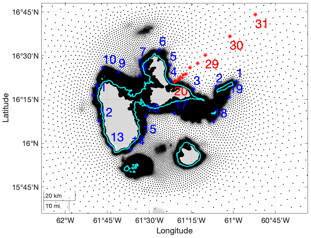
Figure 2 Illustration of the Guadeloupe archipelago (administrative boundaries are outlined in light blue), showing calculation grid points (black dots), the selected numbered locations along the iso-depth contour at 100 m (blue stars), and line transect (red stars). Calculation grid points are more dense in shallow waters. Water depths along the line transect with locations numbered 20–31 are 58, 235, 543, 754, 819, 1206, 1513, 2350, 3265, 4059, 5074, and 5586 m.

To illustrate the SWH data, Fig. 3 depicts the spatial distributions of maximum SWH per location for the four cyclones with the largest single values of SWH in the whole synthetic cyclone database. All cyclones propagate from the southeast to the northwest with intense storm severity near the cyclone track, which reduces quickly away from the track.

Figure 3 Spatial distributions of maximum SWH for the four largest synthetic cyclone events. Each panel gives the maximum SWH (over the period of the cyclone) per location.

3 Methodology

In this section we describe the STM-E methodology used to estimate return values in the current work. Section 3.1 motivates the STM-E approach, and Sect. 3.2 outlines the modelling procedure. Section 3.3 provides a discussion of some of the diagnostic tests performed to ensure that STM-E modelling assumptions are satisfied.

3.1 Motivating the STM-E model

The STM-E procedure has been described in Wada et al. (2018, 2020). The approach is intended to provide straightforward estimation of extreme environments over a spatial region, from a relatively small sample of rare events such as cyclones, the effects of any one of which do not typically influence the whole region. For each cyclone event, the space-time characteristics of the event are summarized using two quantities, the space-time maximum (STM) of the cyclone and the spatial exposure (E) of each location in the region to the event. For any cyclone, the STM is defined as the largest value of SWH observed anywhere in the spatial region for the time period of the cyclone. The location exposure E is defined as the largest value of SWH observed at that location during the time period of the cyclone, expressed as a fraction of STM; thus values of E are in the interval [0, 1].

The key modelling assumptions are then that (i) the future characteristics of STM and E over the region will be the same as those of STM and E during the period of observation, and (ii) in the future, at any location, it is valid to associate any simulated realization of STM (under an extreme value model based on historical STM data) with any realization of E (under a model for the distribution of E based on historical exposure data).

3.2 STM-E procedure

The steps of the modelling procedure are now described. The first three steps of the procedure involve isolation of data for analysis. (a) An appropriate region of ocean is selected. The characteristics of this region need to be such that the underpinning conditions of the STM-E approach are satisfied (as discussed further in Sect. 3.3). (b) For each tropical cyclone event occurring in the region, the largest value of SWH observed anywhere in the region for the period of the cyclone (STM) is retained. (c) Per location in the region, the largest value of SWH observed during the period of the cyclone, expressed as a fraction of STM, is retained as the location exposure E to the cyclone.

The next three steps of the analysis involve statistical modelling and simulation. (d) First, an extreme value model is estimated using the largest values from the sample of STM; typically, a generalized Pareto distribution (see for example Coles, 2001) is assumed. Then a model for the distribution of location exposure E is sought; typically we simply re-sample at random with replacement from the values of historical exposures for the location, although model fitting is also possible. (e) Next, realizations of random occurrences of STM from (d), each combined with a randomly sampled exposure E per location, permit estimation of the spatial distribution of SWH corresponding to return periods of arbitrary length. (f) Finally, diagnostic tools are used to confirm the consistency of simulations (e) under the model with historical cyclone characteristics.

3.3 Diagnostics for STM-E modelling assumptions

The success of the current approach critically relies on our ability to show that simplifying assumptions regarding the characteristics of STM and exposure are justified for the data at hand. In particular, the approach assumes that (i) the distribution STM does not depend on cyclone track, environmental covariates, space, and time, and (ii) the distribution of exposure per location does not depend on STM, cyclone track, environmental covariates, and time. Diagnostic tests are undertaken to examine the plausibility of these conditions for the region of ocean of interest for each application undertaken. Establishing the validity of the STM-E conditions is vital for credible estimation of return values. Section 5 of Wada et al. (2018) provides a detailed discussion of diagnostic tests that should be considered to judge that the STM-E conditions are not violated in any particular application. For example, the absence of a spatial trend in STM over the region can be assessed by quantifying the size of linear trends in STM along transects with arbitrary orientation in the region. This is then compared with a “null” distribution for linear trend, estimated using random permutations of the STM values. Illustrations of some of the diagnostic tests performed for the current analysis are given in Sect. 4 below.

Return value estimates from STM-E are also potentially sensitive to the choice of region for analysis. We assume that the extremal behaviour of STM can be considered homogeneous in the region, suggesting that the region should be sufficiently small that the same physics is active throughout it. However, the region also needs to contain sufficient evidence for cyclone events and their characteristics to allow reasonable estimation of tails of distributions for SWH per location. The absence of dependence between STM and E per location can be assessed by calculating the rank correlation between STM (S, a space-time maximum) and exposure (E_j, at location j, for locations j=1, 2, …, p) using Kendall's τ statistic. If the values of S and E_j increase together, the value of Kendall's τ statistic will be near unity. If there is no particular relationship between S and E_j, the value of Kendall's τ will be near zero. For large n, if S and E_j are independent, the value of Kendall's τ is approximately Gaussian-distributed with zero mean and known variance, providing a means of identifying unusual values which may indicate dependence between S and E_j. An illustrative spatial plot of Kendall's τ is given in Sect. 4.

Finally, estimates from STM-E are potentially sensitive to the extreme value threshold ψ_n (or equivalently the sample size n of the largest observations of STM) chosen to estimate the tail of the distribution of STM over the region. Results in Sect. 4 are reported for a number of choices of n for this reason.

3.4 Modelling STM and estimating return values

Suppose we have isolated a set of n₀ values of STM using the procedure above. We use the largest n≤n₀ values $\mathit{\{}{s}_i{\mathit{\}}}_{i=\mathrm{1}}^n$, corresponding to exceedances of threshold ψ_n, to estimate a generalized Pareto model for STM, with the probability density function

$$\begin{array}{}\text{(1)}& \begin{array}{rl}\mathrm{Pr}\left(S\le s|S>{\mathit{\psi }}_n\right)& =F_{\mathrm{S}|{\mathit{\psi }}_{\mathrm{S}}}\left(s\right)\stackrel{\mathrm{large}{\mathit{\psi }}_n}{\approx }{F}_{\mathrm{GP}}\left(s\right)\\ & =\mathrm{1}-{\left(\mathrm{1}+{\displaystyle \frac{\mathit{\xi }}{{\mathit{\sigma }}_n}}\left(s-{\mathit{\psi }}_n\right)\right)}^{-\mathrm{1}/\mathit{\xi }}\mathrm{for}\mathit{\xi }\ne \mathrm{0}\\ & =\mathrm{1}-\exp \left(-{\displaystyle \frac{\mathrm{1}}{{\mathit{\sigma }}_n}}\left(s-{\mathit{\psi }}_n\right)\right)\mathrm{otherwise},\end{array}\end{array}$$

with shape parameter ξ∈ℝ and scale parameter σ_n>0. Choice of n is important to ensure reasonable model fit and bias-variance trade-off. The estimated value of ξ should be approximately constant as a function of n for sufficiently large ψ_n and hence small n. The full distribution F_S(s) of STM can then be estimated using

$$\begin{array}{}\text{(2)}& F_{\mathrm{S}}\left(s\right)=\left\{\begin{array}{ll}{F}_n^{*}\left(s\right)& \mathrm{for}s\le {\mathit{\psi }}_n\\ {\mathit{\tau }}_n+\left(\mathrm{1}-{\mathit{\tau }}_n\right)F_{\mathrm{S}|{\mathit{\psi }}_n}\left(s\right)& \mathrm{otherwise},\end{array}\right.\end{array}$$

where $F_n^{*}\left(s\right)$ is an empirical “counting” estimate below threshold ψ_n, and τ_n is the non-exceedance probability corresponding the ψ_n, again estimated empirically.

Using this model, we can simulate future values H_j of SWH at any location j (j=1, 2, …, p) in the region, relatively straightforwardly. Suppose that E_j is the location exposure at location j, and $F_{{\mathrm{E}}_j}$ is its cumulative distribution function, estimated empirically. Since then $H_j=E_j\times S$, the cumulative distribution function of H_j can be estimated using

$$\begin{array}{}\text{(3)}& \begin{array}{rl}{F}_{H_j}\left(h\right)& =\mathbb{P}\left(H_j\le h\right)\\ & =\underset{s}{\int }\mathbb{P}\left(E_{j}S\le h|S=s\right)f_{\mathrm{S}}\left(s\right)\mathrm{d}s\\ & =\underset{s}{\int }\mathbb{P}\left(E_j\le h/s\right)f_{\mathrm{S}}\left(s\right)\mathrm{d}s\\ & =\underset{s}{\int }{F}_{{\mathrm{E}}_j}(h/s)f_{\mathrm{S}}\left(s\right)\mathrm{d}s,\end{array}\end{array}$$

where f_S(s) is the probability density function of STM, corresponding to cumulative distribution function F_S(s) estimated in Eq. (2).

4 Application of STM-E to cyclone SWH near Guadeloupe

The STM-E methodology outlined in Sect. 3 is applied to data for the neighbourhood of Guadeloupe's main island pair described in Sect. 2. The objective of the analysis is to estimate the T-year return value for SWH from T₀ years of data – for (T₀, T) pairs (200, 500) and (50, 100). First, details of the set-up of the STM-E analysis are provided in Sect. 4.1. Then, in Sect. 4.2, we describe two competitor methods included for comparison with STM-E. Section 4.3 then describes estimates for the 500-year return value on the 100 m iso-depth contour around Guadeloupe's main island pair and the line transect introduced in Sect. 2, illustrated in Fig. 2, using maximum likelihood estimation (see for example Hosking and Wallis, 1987; Davison, 2003). For comparison, Sect. 4.4 then provides estimates obtained using probability-weighted moments (see for example Furrer and Naveau, 2007; de Zea Bermudez and Kotz, 2010a, b). Section 4.5 describes some of the diagnostic tests undertaken to confirm that the fitted model is reasonable. Section 4.6 outlines the inference for the T=100-year return value from data corresponding to T₀=50 years.

4.1 Details of STM-E application

The spatial region of interest is the neighbourhood of Guadeloupe's main island pair in the Caribbean Sea, corresponding to the approximate longitudes 12–18^∘ N and latitudes 58–65^∘ W (see Fig. 1). An initial analysis using Kendall's τ suggests the full region (9.5–18.3^∘ N, 45–65^∘ W) shows dependency of STM and exposure, with stronger cyclones tending to pass through the western part of the region. However, if a very high threshold ψ≈20 m were to be selected for analysis, reasonable decoupling of STM and E could be achieved, with relatively less intense tropical cyclones neglected. Since the focus of the current work is the ocean environment of the Guadeloupe archipelago, a smaller region (see Fig. 1, right panel) was defined. For this region, Kendall's τ indicated low dependence between STM and E for thresholds ψ of 10 m and above, as illustrated in the left panel of Fig. 4.

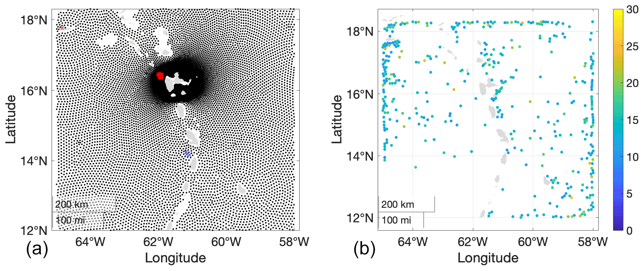
Figure 4 Diagnostics for STM-E. (a) Plot of Kendall's τ for analysis region using a threshold of 10 m. Each point corresponds to a location where SWH data are available and water depth exceeds 100 m. The black dots indicate values of Kendall's τ within the 90 % confidence interval. Red (blue) crosses indicate positive (negative) values of Kendall's τ exceeding the 90 % confidence band. The percentage of recorded exceedances of the 90 % confidence band for Kendall's τ is less than 10 %. (b) Locations of all STMs exceeding 10 m coloured by size of STM in metres.

The right panel of Fig. 4 shows the location and magnitude of STM for each of the n=60 largest cyclones observed in the region. There is no obvious spatial dependence between the size of STM and its location. In Sect. 3.3, we discuss the use of rank correlation of STM along latitude–longitude transects as a means to quantify dependence in general. In fact, the Kendall's τ analysis illustrated in the left panel would also indicate any strong spatial dependence in STM; therefore, results of the rank correlation analysis along latitude–longitude transects are not presented. We conclude that Fig. 4 does not suggest that the modelling assumptions underlying STM-E are not satisfied.

The relatively large number of boundary STM values reflects occurrences of cyclones, the true STM locations of which occur outside the analysis region. For these events, the value of STM used for analysis is the largest value of SWH observed within the analysis region. In this sense, we are performing the STM-E analysis conditional on the choice of region. For example, consider a cyclone for which the location of the STM value s^* falls outside the region of interest. Then the conditional STM value s for the cyclone (within the region) will of course be smaller than s^*; however, the cyclone's conditional exposure (assessed relative to the conditional STM s for the region, rather than the full STM s^*) will consequently be larger.

Specific interest lies in the variation in the extreme return value around Guadeloupe and the rate of increase in return value with increasing water depth away from the coasts. It is known that SWH at a location is dependent on water depth, bathymetry, and coastlines, since ocean waves in shallow water for example are influenced by bottom effects, and since both wind and wave propagation can be weakened in the vicinity of coastlines. For this reason, two sets of locations were adopted for the detailed analysis reported here. The first set corresponds to 19 locations on an approximately iso-depth contour at 100 m depth around the main island pair of Guadeloupe. This depth value is typically chosen to define the boundaries of the local-scale high-resolution flooding simulations. The second set corresponds to 12 locations on a line transect emerging approximately normally from the northeast of the main island pair of Guadeloupe. We focus on the northeast neighbourhood, because it has the highest exposure to cyclones. The contour and transect are illustrated in Fig. 2, and location numbers are listed.

The focus of the analysis is estimation of the T=500-year return value for SWH on the iso-depth contour and line transect, based on T₀=200 years of data. To quantify the uncertainty in the 500-year return value using STM-E analysis, the following procedure was adopted. (a) Randomly select the appropriate number of cyclones (corresponding to T₀ years of observation) from the T_L years of synthetic cyclones. (b) Identify the largest n values of STM in the sample, for n=20, 30, 40, 50, and 60 (corresponding to lowering the extreme value threshold). (c) Estimate a model for the distribution of STM using maximum likelihood estimation or the method of probability-weighted moments. (d) Estimate the empirical distribution of exposure E per location on the iso-depth contour and line transect. (e) Estimate the 500-year return value as the quantile of the distribution $F_{{\mathrm{H}}_j}$ of significant wave height at location j with non-exceedance probability $\mathrm{1}-(T_{\mathrm{0}}/n)/T$. Finally, the whole procedure (a)–(e) is repeated 100 times to quantify the uncertainty in the T-year return value.

Figure 5 illustrates the tails of the distribution of STM from the largest 30 values of STM from each of 100 random samples corresponding to 200 years, and from the full sample of synthetic cyclones. It can be seen that the 500-year return value for STM lies in the region (20, 30) m.

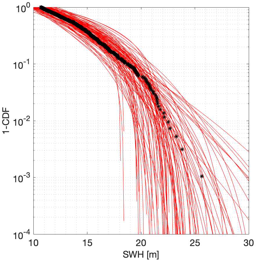
Figure 5 Variability of tail of distributions for STM on log scale. Each of the 100 red lines is estimated from a sample size of 30 of largest STM values from a random sample of 124 cyclones corresponding to 200 years of observation. The black points indicate the corresponding empirical distribution of STM from the full synthetic cyclone data.

4.2 Benchmarking against the full cyclone database and single-location analysis

One obvious feature of the current synthetic cyclone database is that it corresponds to a long time period relative of T_F=3200 years, much longer than the return period of T=500 years being estimated in the current analysis. Thus, we are able to estimate the 500-year return value at any location using the full synthetic cyclone data, by simply interpolating the sixth and seventh largest values, corresponding to the non-exceedance probability in 500 years. This provides a direct empirical estimate.

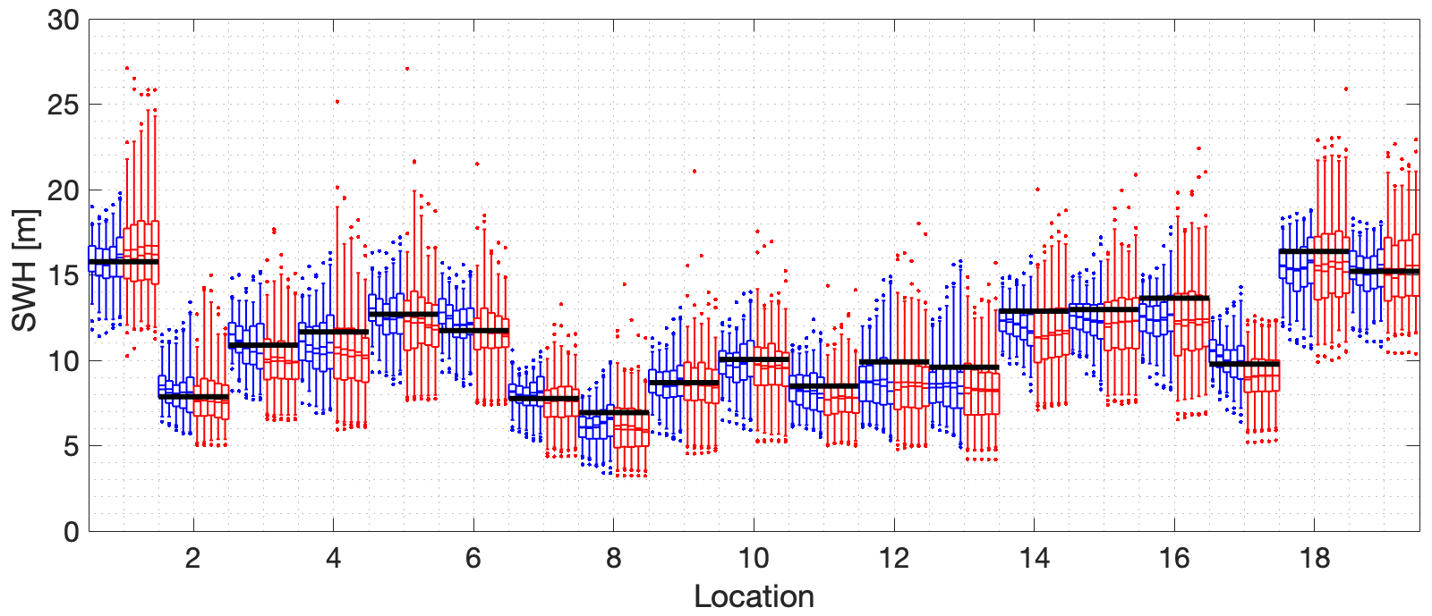
Figure 6 The 500-year return value for SWH using maximum likelihood estimation for the 100 m iso-depth contour. The x axis gives the reference numbers of the 19 locations on the contour. Location numbers are given in Fig. 2. Corresponding to each location, the blue box–whiskers summarize the estimated return value from STM-E for different sample sizes 20, 30, 40, 50, and 60; the red box–whiskers summarize the estimated return values from single-location analysis for different sample sizes. For each blue and red cluster of box–whiskers corresponding to a specific location, return value estimates for the increasing sequence of sample sizes are plotted sequentially outwards from the centre of the cluster. For all box–whiskers, the box represents the inter-quartile interval, and the median and mean are shown as solid and dashed lines. Whiskers represent the 2.5 % to 97.5 % interval. Exceedances of this 95 % interval are shown as dots. The black horizontal line for each location corresponds to the empirical estimate of the return value obtained directly from the full synthetic cyclone data for that location.

From previous work, a key advantage found using the STM-E approach is that it provides less uncertain estimates at a location compared with conventional single-location analysis. We wish to demonstrate in the current work that this is also the case. For this reason, we also calculate estimates for comparison with those from STM-E, based on independent analysis of cyclone data from each location of interest.

4.3 Maximum likelihood estimation

Figure 6 illustrates the 500-year return value for SWH using maximum likelihood estimation for locations on the 100 m iso-depth contour around Guadeloupe's main island pair, with location numbers given in Fig. 2. The figure caption gives relevant details of the figure layout. Across the 19 locations considered, the 500-year return value is estimated using STM-E (blue), single-location (red), and full synthetic cyclone data (black); in general, there is good agreement between estimates per location. Bias characteristics for single-location and STM-E estimates are relatively similar in general. It can be seen however (from the longer red whiskers) that the uncertainty in single-location estimates is greater in general from the corresponding STM-E estimates.

As the number of points used for STM-E estimation per location increases, there is evidence for reduction in the uncertainty with which the return value is estimated, as might be expected. However, there is also some evidence for a small increase in the mean estimated return value. This is explored further in Sect. 4.5. There is very little corresponding evidence for reduced uncertainty in the single-location analysis. There are more outlying estimates of return value for single-location analysis than for STM-E.

The corresponding results for the line transect analysis using maximum likelihood estimation is given in Fig. 7. The general characteristics of this figure are similar to those of Fig. 6. The return value increases as would be expected with increasing water depth. Single-point estimates are more variable that those from STM-E. Biases appear to be relatively small and similar for STM-E and single-location estimates. There is little evidence that the STM-E median estimate increases with increasing sample size. We infer from the analysis that water depth has little effect on the performance of the STM-E approach.

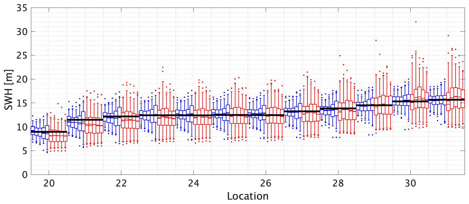
Figure 7 The 500-year return value for SWH using maximum likelihood estimation for the line transect. The x axis gives the reference numbers of the 12 locations on the transect. Briefly, for each location, blue and red box–whiskers summarize the estimated return value from STM-E and single-location analysis respectively; see caption of Fig. 6 for other details. The black horizontal lines for each location correspond to the empirical estimate of the return value obtained directly from the full synthetic cyclone data for that location. Water depths at the 12 line transect locations are given in the caption to Fig. 2.

4.4 Results estimated using probability-weighted moments

Estimates for the 500-year return value on the iso-depth contour, obtained using the method of probability-weighted moments, are shown in Fig. 8. The behaviour of STM-E and single-location estimates shown is very similar to that illustrated for maximum likelihood estimation in Fig. 6.

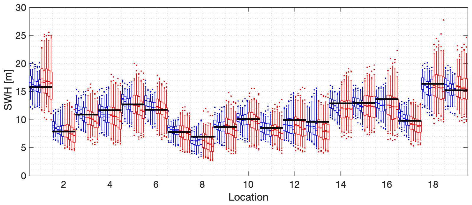
Figure 8 The 500-year return value for SWH estimated using probability-weighted moments for the 100 m depth contour. The x axis gives the reference numbers of the 19 locations on the contour. Briefly, for each location, blue and red box–whiskers summarize the estimated return value from STM-E and single-location analysis respectively; see caption of Fig. 6 for other details. The black horizontal lines for each location correspond to the empirical estimate of the return value obtained directly from the full synthetic cyclone data for each location.

Results for the line transect using probability-weighted moments are given in Fig. 9; again, the figure shows similar trends to Fig. 7. There is some evidence that the STM-E median estimate increases with increasing sample size and that this reduces bias.

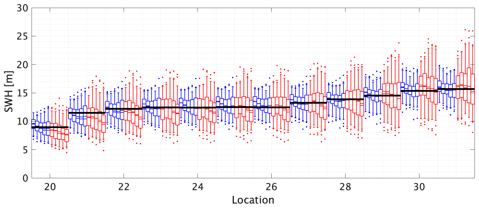
Figure 9 The 500-year return value for SWH estimated using probability-weighted moments for the line transect. The x axis gives the reference numbers of the 12 locations on the transect. Briefly, for each location, blue and red box–whiskers summarize the estimated return value from STM-E and single-location analysis respectively; see caption of Fig. 6 for other details. The black horizontal lines for each location correspond to the empirical estimate of the return value obtained directly from the full synthetic cyclone data for each location. Water depths at the 12 line transect locations are given in the caption to Fig. 2.

4.5 Assessment of model performance

Comparing box–whisker plots from centre to left for each location in the figures in Sect. 4.3 and 4.4 suggests that there is sometimes a small increasing trend in return value estimates from STM-E as a function of increasing sample size for inference. We investigate the trend further here. Figure 10 gives estimates for the 500-year return value of space-time maximum STM (as opposed to the full STM-E estimate for SWH) as a function of sample size used for estimation, using maximum likelihood estimation (blue) and probability-weighted moments (red). Also shown in black is the empirical estimate of the 500-year STM return value obtained directly from the synthetic cyclone data. The figure shows a number of interesting effects. Firstly, STM estimates from both maximum likelihood and the probability-weighted moments increase with increasing sample size n, and this effect is more pronounced for probability-weighted moments. As a result, the bias of estimates using probability-weighted moments is considerably larger than that from maximum likelihood estimation for sample size of 60. The uncertainty of estimates from probability-weighted moments is also somewhat larger than that from STM-E.

Figure 10 The effect of sample size on estimates of return values for STM. Box–whiskers summarize estimates for the 500-year STM return value based on maximum likelihood estimation (blue) and the method of probability-weighted moments (red), for different sample sizes. The black dashed line gives an empirical estimate of the return value obtained directly from the synthetic cyclone data.

A number of studies in the literature compare the performance of different methods of estimation of extreme value models. The method of probability-weighted moments is known to perform relatively well relative to maximum likelihood estimation for small samples (see for example Jonathan et al., 2021, Sect. 7 for a discussion). For small samples, for example, maximum likelihood estimation is known to underestimate the generalized Pareto shape parameter and over-estimate the corresponding scale parameter, leading to bias in return value estimates. The results in Fig. 10 indicate that, if anything, maximum likelihood estimation performs somewhat better than the method of probability-weighted moments for the current application. Regardless, the trends in Fig. 10 serve to illustrate the importance of performing the STM extreme value analysis with great care, particularly for small sample sizes.

One of the assumptions underpinning the STM-E approach is that the exposure distribution at a location is not dependent on the magnitude of STM. We investigate this further here. Our aim is to show that the empirical cumulative distribution function for exposure (henceforth ECDF for brevity) corresponding to the largest and smallest STMs is typical of ECDFs in general and are in no way special relative to ECDFs corresponding to other cyclones. We can quantify the difference between two ECDFs using the Kullback–Leibler divergence (KL) (Liese and Vajda, 2006). We proceed to estimate the “null” distribution of KL using 1000 sets of randomly selected pairs of ECDFs. In addition, we calculate the Kullback–Leibler divergence KL^* for the pair of ECDFs corresponding to cyclones with the largest and smallest STMs. If there is no dependence of ECDF on STM, then the value of KL^* should correspond to a random draw from the null distribution of KL. The left-hand panel of Fig. 11 illustrates the null distribution of KL at Location 21, for a sample size of 20, together with the corresponding value of KL^*. We note that the value of KL^* is not extreme in the null distribution. In the right-hand panel of Fig. 11, the empirical cumulative distribution function of the non-exceedance probability of KL^* (in the corresponding null distribution) is estimated over all locations and sample sizes. The approximate uniform density found suggests indeed that KL^* corresponds to a random draw from the null distribution; a Kolmogorov–Smirnov test on the data suggested that it was not significantly different to a random sample from a uniform distribution on [0, 1].

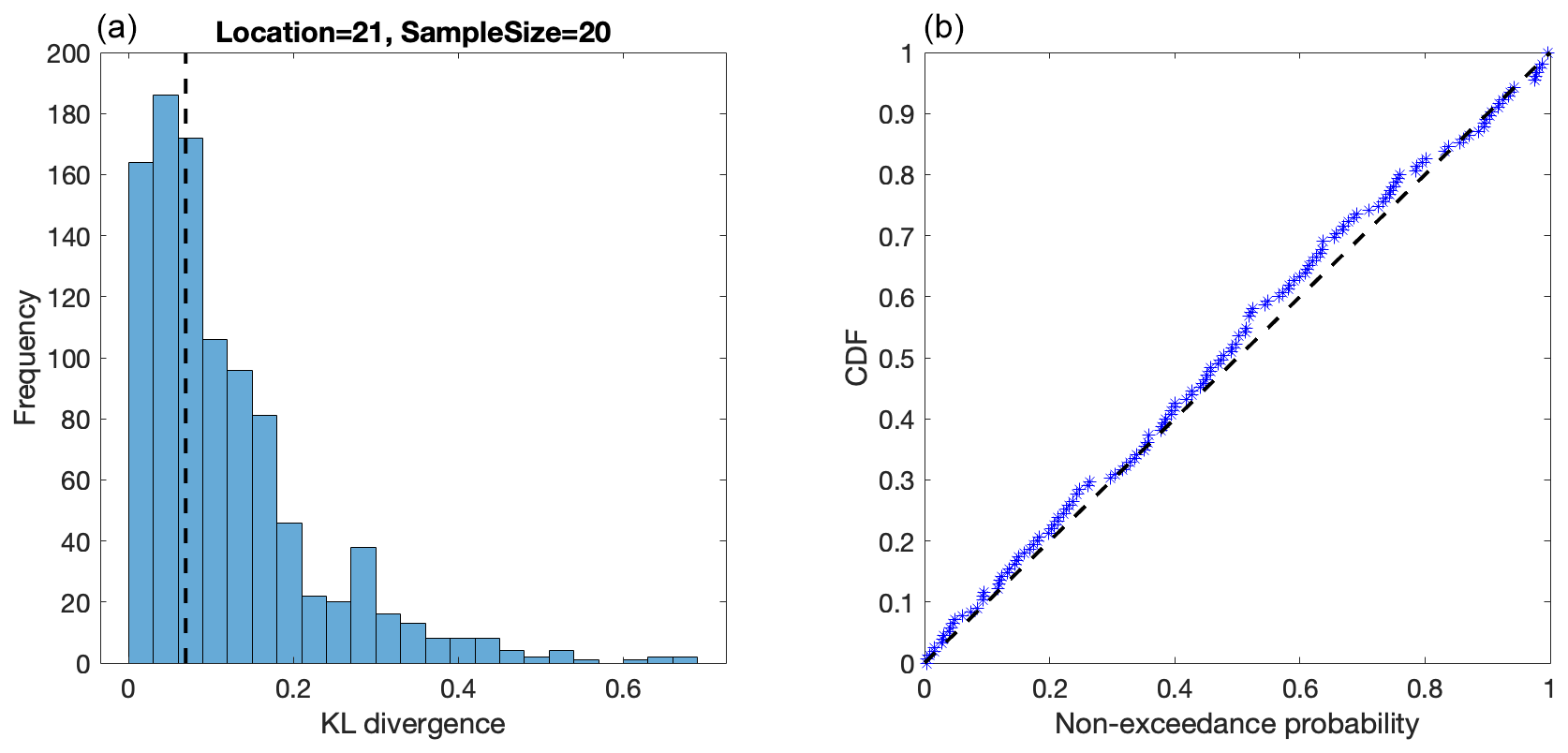
Figure 11 (a) Histogram of KL from random pairs of empirical distribution functions for exposure (corresponding to the “null” distribution of KL), together with KL^* for Location 21 with a sample size of 20. (B) QQ plot of the non-exceedance probability of KL^* (in the corresponding null distribution for KL) over all locations and sample sizes.

Complementary analyses (not shown) evaluated KL^* for ECDFs corresponding to the largest two STMs in the data and (separately) for ECDFs corresponding to the smallest two STMs. Results again indicated that both of these choices for KL^* could be viewed as random in their null distributions. Since exposure distribution at a location is not dependent on the magnitude of STM, we assume the overall performance of STM-E is mainly governed by the estimation of STM. In shallow water, where waves are subject to breaking, it would be expected that the exposure distribution would be dependent on STM, and therefore the validity of the method should be more carefully checked using the approaches described in Sect. 3.3.

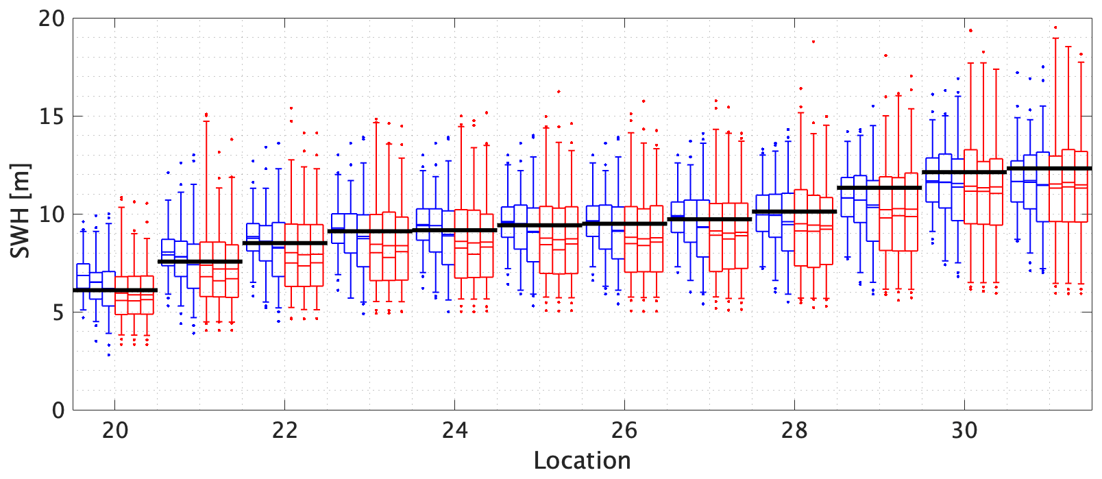
Figure 12 The 100-year return value for SWH using probability-weighted moments for the line transect. The x axis gives the reference numbers of the 12 locations on the transect. Briefly, for each location, blue and red box–whiskers summarize the estimated return value from STM-E and single-location analysis respectively; see caption of Fig. 6 for other details. The black horizontal lines correspond to the empirical estimate of the return value obtained directly from the full synthetic cyclone data for each location. Water depths at the 12 line transect locations are given in the caption to Fig. 2.

4.6 Model performance for smaller sample sizes

Here we repeat the analysis in Sect. 4.1–4.5 above for the T=100-year return value for SWH on the iso-depth contour and line transect, based on T₀=50 years of data. The typical number of tropical cyclone events occurring in 50 years is approximately 30, already corresponding to a very small sample size for extreme value analysis. We retain the largest n values of STM in the sample, for n=10, 15, and 20 for this analysis. The overall performance of STM-E estimates, relative to those from single-location analysis and an empirical estimate from the full synthetic cyclone data, is summarized in Fig. 12 for the line transect, using the method of probability-weighted moments (and see also Table 2 in the next section for a summary including estimates using maximum likelihood). The figure's features are similar to those of figures discussed earlier. Estimates from STM-E show lower bias and reduced uncertainty relative to those from single-location analysis. There is slight underestimation of the return value, but the empirical estimate sits comfortably within the 25 %–75 % uncertainty band (corresponding to the “box” interval). The corresponding plots (not shown) for the iso-depth contour, and for estimation using maximum likelihood, are similar.

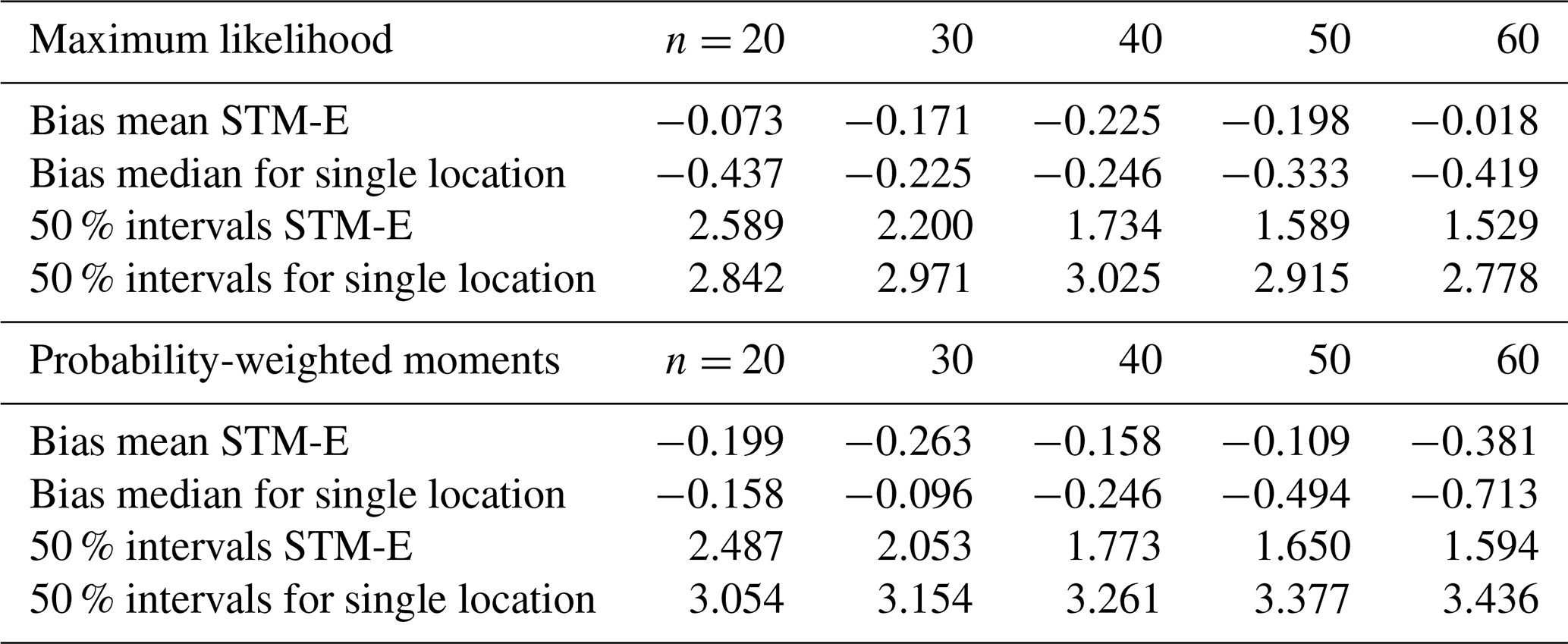
Table 1 Performance of STM-E and single-location analysis in estimation of the bias and uncertainty of the 500-year return value, relative to empirical estimates from the full synthetic cyclone data, for analysis sample sizes of 20, 30, 40, 50, and 60 all extracted from the 200-year data set. Bias B is assessed as the average difference (over the iso-depth contour and line transect analyses) between the mean STM-E (or single-location) estimate and the return value estimate from the full cyclone database. Similarly, uncertainty U is assessed in terms of the average width of the 50 % uncertainty band of the STM-E (or single-location) estimate.

5 Discussion

This work considers the estimation of T-year return values for SWH over a geographic region, from small sets of T₀ years of synthetic tropical cyclone data, using the STM-E (space-time maxima and exposure) methodology. We assess the methodology by comparing estimates of the T-year return value (T>T₀) for locations in the region from STM-E with those estimated directly from a large database corresponding to T_L (>T) years of synthetic cyclones. We find that STM-E provides estimates of the T=500-year return value from T₀=200 years of data in the region of the Guadeloupe archipelago with low bias. We also compare STM-E estimates of T-year return values for locations in the region with those obtained by extreme value analysis of data (for T₀ years) at individual locations. We find that the uncertainty of STM-E estimates is lower than that of single-location estimates. Comparison of the performance of inferences for the T=100-year return value from T₀=50 also suggests STM-E outperforms single-location analysis.

For reasonable application of the STM-E approach, it is important that characteristics of tropical cyclones over the region under consideration satisfy a number of conditions. These conditions are shown not to be violated for a region around the Guadeloupe archipelago but that use of the STM-E method over a larger spatial domain would not be valid (see for example Wada et al., 2019). This demonstrates that selection of an appropriate geographical region for STM-E analysis is critical to its success. Once such a region is specified, we find that STM-E provides a simple but principled approach to return value estimation within the region from small samples of tropical cyclone data.

Return value estimates from STM (see for example Fig. 10) show a small increasing bias with increasing sample size for extreme value estimation. However, the resulting bias in full STM-E return values is small. Corresponding estimates based on single-location analysis also show relatively small but increasing negative bias with increasing sample size. In the present work, the tail of the distribution of STM was estimated by fitting a generalized Pareto model, using either maximum likelihood estimation or the method of probability-weighted moments. Estimates for extreme quantiles of STM using either approach are in good agreement.

Table 1 summarizes the performance of STM-E and single-location analysis in estimation of the bias and uncertainty of the 500-year return value, relative to empirical estimates from the full synthetic cyclone data, for analysis sample sizes of n=20, 30, 40, 50, and 60. Bias B(n;𝙼𝚝𝚑) and uncertainty U(n;𝙼𝚝𝚑) are estimated as average characteristics over all $\left|\mathcal{L}\right|=\mathrm{31}$ locations $\mathrm{\ell }\in \mathcal{L}=\mathit{\{}\mathrm{1},\mathrm{2},\mathrm{\dots },\mathrm{31}\mathit{\}}$ on the iso-depth contour and line transect corresponding to the relevant sample size, using the expressions

$$\begin{array}{}\text{(4)}& \begin{array}{rl}& B(n;\mathtt{\text{Mth}})={\displaystyle \frac{\mathrm{1}}{\left|\mathcal{L}\right|}}\sum _{\mathrm{\ell }\in \mathcal{L}}\left(\stackrel{\mathrm{̃}}{h}(\mathrm{\ell };n,\mathtt{\text{Mth}})-{\stackrel{\mathrm{̃}}{h}}_{\mathrm{0}}(\mathrm{\ell };n)\right),\\ & U(n;\mathtt{\text{Mth}})={\displaystyle \frac{\mathrm{1}}{\left|\mathcal{L}\right|}}\sum _{\mathrm{\ell }\in \mathcal{L}}\left({\displaystyle \frac{r(\mathrm{\ell };n,\mathtt{\text{Mth}})}{r_{\mathrm{0}}(\mathrm{\ell };n)}}-\mathrm{1}\right).\end{array}\end{array}$$

Here, $\stackrel{\mathrm{̃}}{h}(\mathrm{\ell };n,\mathtt{\text{Mth}})$ and ${\stackrel{\mathrm{̃}}{h}}_{\mathrm{0}}\left(n\right)$ correspond to the mean 500-year return value estimated using sample size n from the inference method Mth (either maximum likelihood or probability-weighted moments) and directly from the full synthetic cyclone database; $r(\mathrm{\ell };n,\mathtt{\text{Mth}})$ and r₀(n) are the corresponding 50 % uncertainty bands. The table summarizes the findings presented pictorially in Figs. 6–8. In terms of bias, STM-E and single-location estimates underestimate the return value on average. STM-E is less biased than single-location estimates except for sample sizes of 20 and 30 using probability-weighted moments. STM-E also provides estimates of the 500-year return value with higher precision than the single-location analysis.

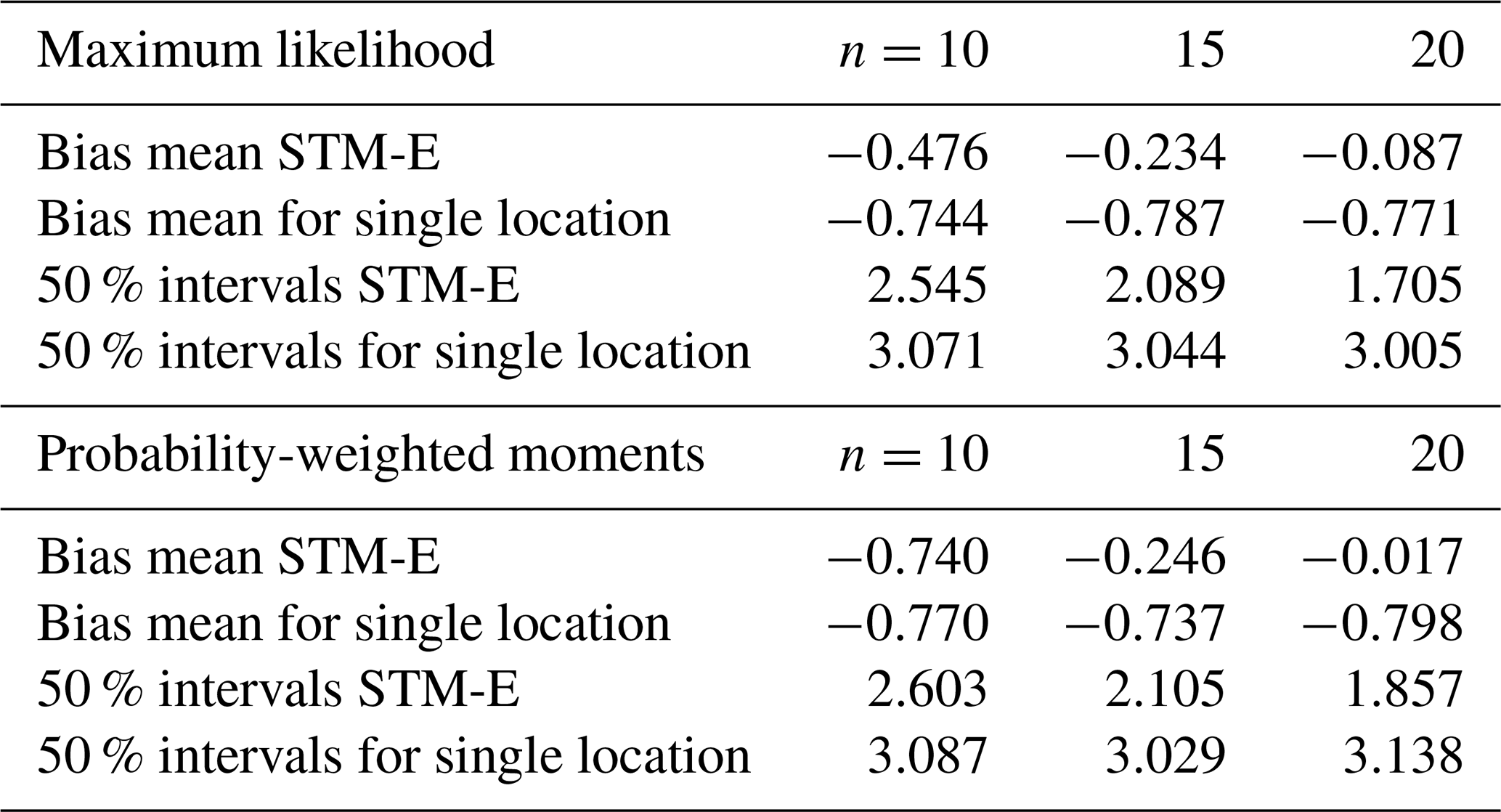
Table 2 provides the corresponding summary for estimation of the T=100-year return value from a sample corresponding to approximately T₀=50 years of data. Features are similar to those of Table 1.

Table 2 Performance of STM-E and single-location analysis in estimation of the bias and uncertainty of the 100-year return value, relative to empirical estimates from the full synthetic cyclone data, for analysis samples of size of 10, 15, and 20 all extracted from the 50-year data set. Bias B is assessed as the average difference (over the iso-depth contour and line transect analyses) between the mean STM-E (or single-location) estimate and return value estimated from the full cyclone data. Similarly, uncertainty U is assessed in terms of the average width of the 50 % uncertainty band of the STM-E (or single-location) estimate.

An appropriate choice of sample size n for STM-E analysis is likely to be related to the size n₀ of the full sample available and the period T₀ to which the sample corresponds. For example, in the current work for T=500 years, n=20 and n₀=124 are approximately equivalent to the largest 15 % of cyclones for the sample period T₀=200 year. That is, the smallest cyclone considered in the n=20 STM-E model has a return period of the order of 10 years. With n=60, we use approximately half the sample for STM-E analysis, and the smallest cyclone in the STM-E analysis has a return period of the order of 3 years. In the case T=100 years, T₀=50, and n₀≈30, we found that STM-E performance was still reasonable using n=12, 15, and 20.

Inferences from the current work confirm the findings of previous studies (Wada et al., 2018, 2020) that STM-E provides improved estimates of return values compared to statistical analysis at a single location. From an operational perspective, STM-E is useful for regions like the southwest Pacific Ocean (McInnes et al., 2014) or Indian Ocean basin (Lecacheux et al., 2012), where cyclone-induced storm wave data are limited. For such locations, STM-E achieves low bias and higher precision and should be preferred to the single-location approach.