Estimating dune erosion at the regional scale using a meta-model based on neural networks

Sandy beaches and dune systems have high recreational and ecological value, and they offer protection against flooding during storms. At the same time, these systems are very vulnerable to storm impacts. Process-based numerical models are presently used to assess the morphological changes of dune and beach systems during storms. However, such models come with high computational costs, hindering their use in real-life applications which demand many simulations and/or involve a large spatial–temporal domain. Here we design a novel meta-model to predict dune erosion volume (DEV) at the Dutch coast, based on artificial neural networks (ANNs), trained with cases from process-based modeling. First, we reduce an initial database of ∼1400 observed sandy profiles along the Dutch coastline to 100 representative typological coastal profiles (TCPs). Next, we synthesize a set of plausible extreme storm events, which reproduces the probability distributions and statistical dependencies of offshore wave and water level records. We choose 100 of these events to simulate the dune response of the 100 TCPs using the process-based model XBeach, resulting in 10 000 cases. Using these cases as training data, we design a two-phase meta-model, comprised of a classifying ANN (which predicts the occurrence (or not) of erosion) and a regression ANN (which gives a DEV prediction). Validation against a benchmark dataset created with XBeach and a sparse set of available dune erosion observations shows high prediction skill with a skill score of 0.82. The meta-model can predict post-storm DEV 10³–10⁴ times faster (depending on the duration of the storm) than running XBeach. Hence, this model may be integrated in early warning systems or allow coastal engineers and managers to upscale storm forcing to dune response investigations to large coastal areas with relative ease.

1 Introduction

Extreme wave and storm-surge conditions induced by tropical or extratropical storms can modify the morphological shape of sandy coasts and dunes dramatically (Vellinga, 1982; McCall et al., 2010; Castelle et al., 2015), with high impacts on local assets, infrastructure, ecosystems or touristic value. More importantly, at dune-protected coasts the partial or total erosion of the dunes during extreme storms can cause flooding of the hinterland (van Dongeren et al., 2018; Almar et al., 2021). The amount of dune erosion is associated with the offshore storm intensity (e.g., maximum wave height and storm surge) but can locally vary for the same storm due to spatial variabilities of pre-storm foreshore and dune morphology and local hydrodynamics (Houser et al., 2008; Athanasiou et al., 2018; Beuzen et al., 2019). Accurate predictions of dune erosion during storms can be critical in early warning systems for the identification of dune erosion hotspots along long coastal stretches, as well as for long-term coastal zone management, aiding in decision making and adaptation strategies to reinforce and/or nourish coasts and dunes.

Conceptual models that identify storm-impact regimes based on simple indicators using the relative elevations between the beach–dune and the total water levels have been previously employed to assess coastal vulnerability at a regional scale (Sallenger, 2000; Stockdon et al., 2007; Leaman et al., 2021). While these simple models provide extremely fast estimations of the expected impact, their output is qualitative, only describing the general scale of impact. Moreover, simple empirical or behavioral models are commonly employed for probabilistic dune erosion risk assessments to enable fast run times (Ranasinghe et al., 2012; Li et al., 2014b; Antolínez et al., 2019). However, their accuracy and adaptability can be limited due to their simplifications. On the other hand, process-based models, like XBeach (Roelvink et al., 2009), have shown great skill in reproducing morphological changes in the dune system during storms (Lindemer et al., 2010; McCall et al., 2010; Vousdoukas et al., 2011; de Winter et al., 2015; Passeri et al., 2018) but are computationally demanding. This can become particularly problematic for large spatial scales or when a large number of simulations is needed, hindering their application in early warning systems or probabilistic risk assessments. To this end, data-driven methods based on statistical approaches can provide a good alternative to achieve faster estimations. Since dune erosion observations (with large spatial and temporal coverage) are scarce, a common approach is to generate synthetic data of dune erosion based on plausible storm conditions using process-based modeling (Poelhekke et al., 2016; Pearson et al., 2017; Santos et al., 2019). Among the most used data-driven methods in coastal applications are Bayesian networks (Gutierrez et al., 2011; Poelhekke et al., 2016; Beuzen et al., 2017; Giardino et al., 2019; Sanuy and Jiménez, 2021), which use conditional probabilities between system parameters to study cause and effect. While they can provide useful information on system dependencies (Beuzen et al., 2019), their shortcoming lies in the mandatory discretization of the parameters and their tendency for overfitting when used as predictive tools (Beuzen et al., 2018).

In the last decade, artificial neural networks (ANNs) have been increasingly employed in coastal engineering and management applications due to their effectiveness in modeling complex non-linear systems with great speed. ANNs have been employed for predictions of beach seasonal changes (Hashemi et al., 2010), longshore sediment transport (Kabiri-Samani et al., 2011; Güner et al., 2013), sandbar characteristics (Kömürcü et al., 2013; López et al., 2017), storm surge (Kim et al., 2015) and coastal overtopping (van Gent et al., 2007; Verhaeghe et al., 2008; Chondros et al., 2021). Of particular relevance to this study, Santos et al. (2019) tested the use of ANNs, among other statistical models, to predict changes in dune geometry during storms at Dauphin Island in the USA. Due to the manageable size of the region of interest (∼14 km), they simulated dune response with a 2D XBeach model, and they developed an ANN for each of the 200 transects they studied using only storm conditions as the ANN input parameters. However, since these ANNs were bound to the pre-storm morphology of the individual transects, they cannot be used for different beach and dune morphologies.

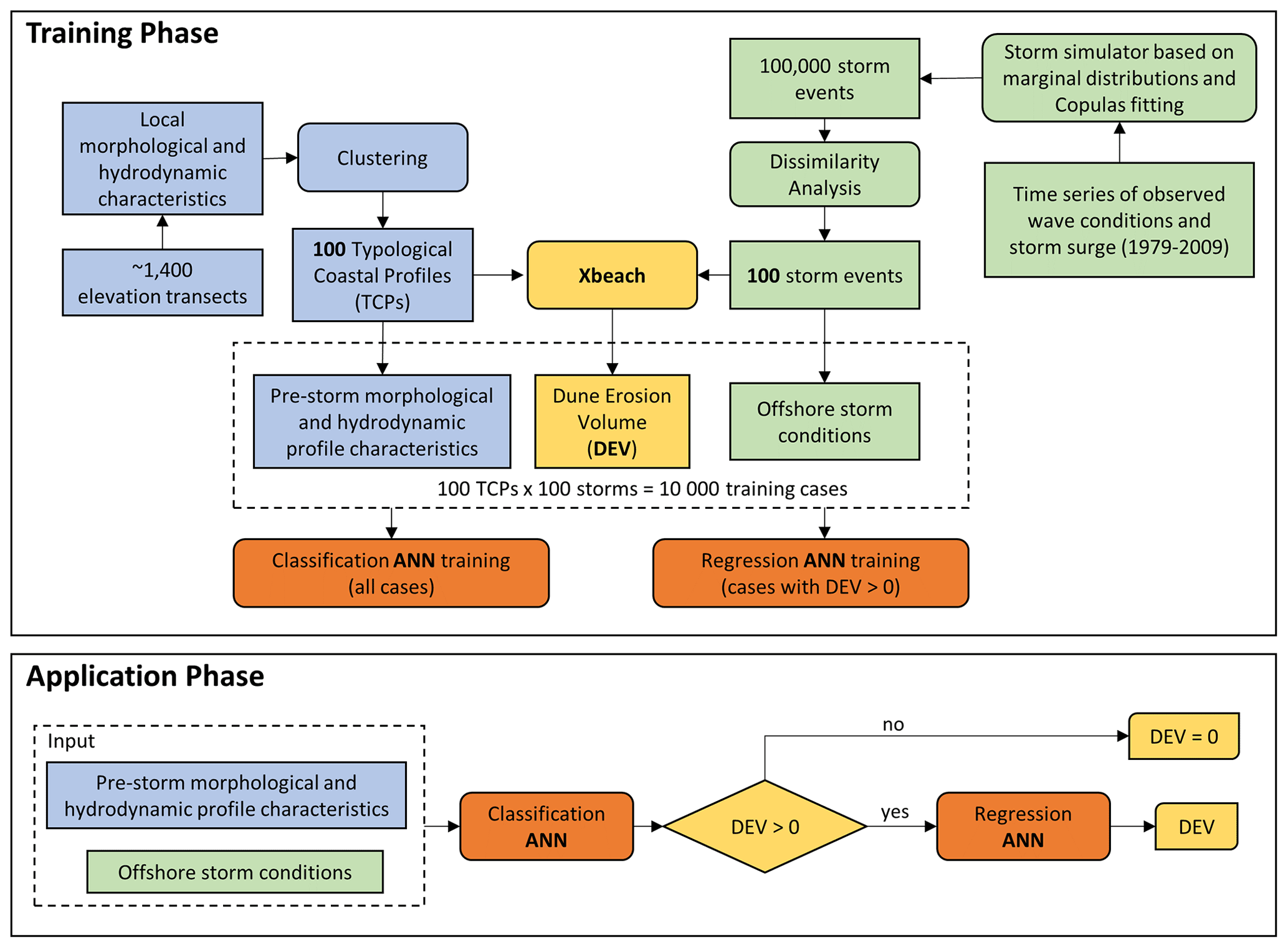
Figure 1 Overview of the training and application of the proposed meta-model for dune erosion volume (DEV) predictions. Blue colors indicate the steps associated with the profile characteristics, green colors the steps related to the offshore storm conditions, yellow colors the steps connected with dune response and orange colors the steps connected with artificial neural networks.

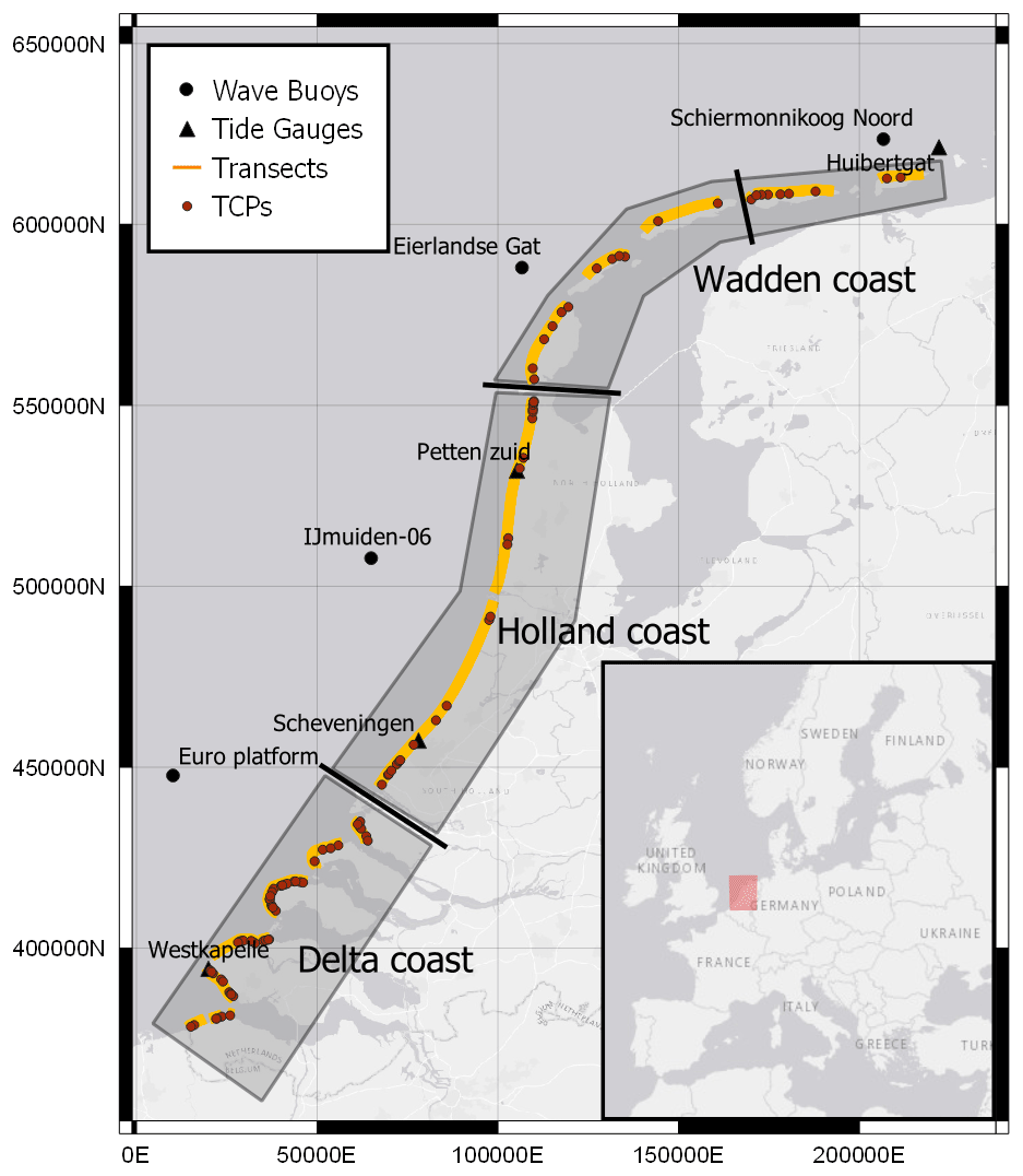
Figure 2 Map of the Dutch coast indicating the location of the JARKUS transects (yellow lines), the offshore stations (wave buoys and tide gauges, black circles and triangles, respectively), and the 100 typological coastal profiles (TCPs, red dots) used as the training dataset in the present study. The thick black lines perpendicular to the coastline separate the different Dutch coastal areas, each one associated with one offshore station. The map is projected on the “Amersfoort/RD New” coordinate system (EPSG: 28992) with the x and y axis in meters. The basemap shown is obtained from ESRI (ESRI, 2011).

Here, we present a meta-model based on ANNs for the prediction of dune erosion volume (DEV) during storms at any location on the Dutch coast (∼260 km of dune fronted coastline) (see Fig. 1). The novelty of the proposed meta-model relative to previous similar methodologies is the inclusion of the pre-storm beach profile as input, which allows for large-scale applications. The model was trained based on a synthetic dataset created with XBeach 1D models, for a large number of cases with combinations of different coastal morphology and storm conditions. To ensure that the training data sufficiently capture the variability in the observed coastal morphology and possible storm conditions while keeping the computational costs for the creation of the synthetic dataset at a manageable level, input reduction techniques and probabilistic analysis were used. First, using clustering techniques, a set of 100 representative typological coastal profiles (TCPs) were chosen from ∼1400 available elevation transects at the Dutch coast based on local morphological and hydrodynamic characteristics (Athanasiou et al., 2021). Then, a simulator of synthetic and physically realistic offshore storm events was developed using marginal distribution and copula fitting methods on the observed storm variables along the Dutch coast. Using a dissimilarity analysis, 100 storm events were chosen per station which were used to force XBeach models for each of the 100 TCPs. The pre-storm morphological and hydrodynamic profile characteristics of each TCP, the offshore storm conditions, and the simulated DEV were used to create a training dataset with 10 000 cases. Using the developed training dataset, a two-phase ANN meta-model was created, which used the pre-storm profile characteristics and offshore storm conditions as inputs and provides a DEV estimate as output. The two phases of the meta-model are composed of (1) a classifier, which estimates if there is dune erosion (DEV >0) or not (DEV =0), and (2) a regressor, which estimates DEV in the case that the classifier predicts dune erosion. Different ANN configurations were tested using a benchmark dataset based on XBeach simulations, and the predictions of the final ANN configuration were compared against observed DEV during three historic storms.

Section 2 describes the methods used to create the representative training dataset and the development of the two-phase ANN meta-model. The optimum configurations of the ANNs and their error statistics are presented in Sect. 3. In Sect. 4, the limitations of the presented methodology and potential applications are discussed. Finally, a summary of the main conclusions of the work is presented in Sect. 5.

2 Methods

2.1 Case study and data availability

The Dutch coast, located at the North Sea, has a total length of 432 km, including (1) the Delta region in the south, composed of islands and estuaries; (2) the Holland coast in the center, with long stretches of sandy beaches and dunes; and (3) the Wadden islands in the north, comprising barrier islands and tidal inlets (Fig. 2). Almost 60 % of the total coastline comprises of beach and dune systems (Ruessink and Jeuken, 2002), which form part of the coastal defenses protecting the low-lying hinterland from flooding. Depth and elevation measurements are available on an annual basis (taking place between April and September) at fixed transects along the Dutch coast through the JARKUS (“Jaarlijkse Kustmeting”, annual coastal measurement) program.

Time series of wave conditions (significant wave height H_s, peak wave period T_p and mean direction “Dir”) at 3-hourly intervals are available between 1979 and 2009 from directional wave-rider buoys at four offshore locations at depths of about 25 m on average (Fig. 2). Additionally, water level time series at 10 min intervals are available from four tide gauges along the coast (Fig. 2), for which a tidal analysis was performed in Athanasiou et al. (2021) and the local tide and storm surge level (SSL, difference between water level and tidal level) were extracted. The wave and water level time series are available from Rijkswaterstaat, an agency of the Ministry of Infrastructure and Water Management of the Netherlands.

In Athanasiou et al. (2021) 1430 of the JARKUS transects which represent sandy beach and dune systems, were chosen and the elevation profiles were extracted for the year 2019. In that study, various morphological and hydrodynamic parameters were calculated per profile and episodic dune erosion volume was simulated per profile with the process-based model XBeach for 10 representative storms.

2.2 Typological coastal profiles

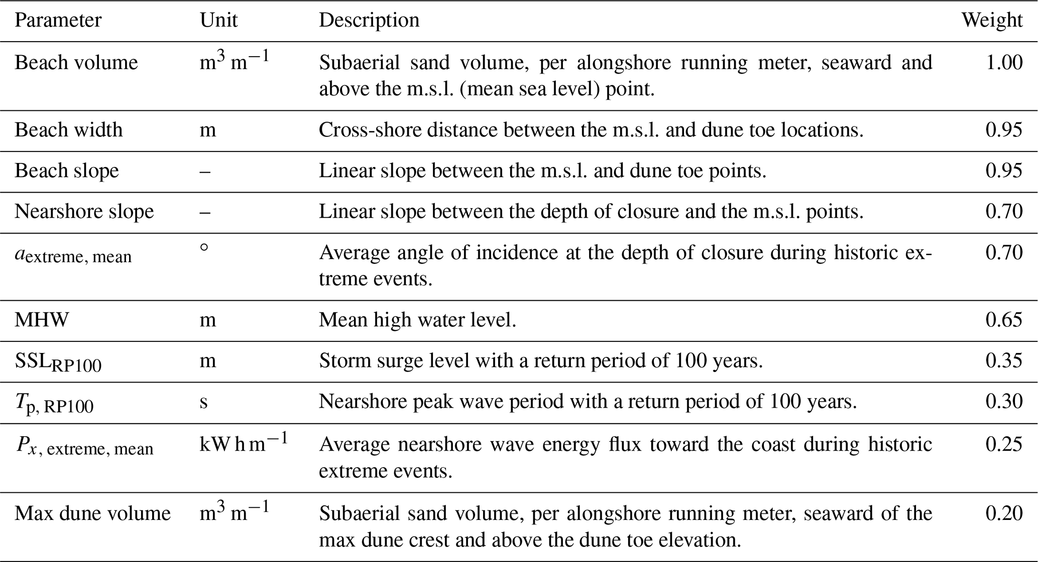
A two-phase clustering approach similar to that in Athanasiou et al. (2021) was applied to group the available profiles into 100 clusters based on their similarities, each described by its representative profile (centroid) called a typological coastal profile (TCP) (red dots in Fig. 2). We excluded some of the 1430 profiles from Athanasiou et al. (2021), which were found to be at highly dynamic areas (e.g., transect at the tips of the Wadden islands where no clear dune features were identified) or transects at the non-exposed side of the Wadden islands, leaving 1368 transect for our study. The 1368 profiles were first clustered into 300 initial groups, leading to 300 initial TCPs, based on a set of 10 morphological and hydrodynamic parameters that characterize each profile (Table 1). Then a second clustering was performed on the 300 initial TCPs, where their simulated dune response to 10 different storms was taken into account, to group them in 100 clusters and obtain the final TCPs. For detailed information on the exact methodology we refer to Athanasiou et al. (2021). Most of the resulting TCPs were located at the Delta coast (∼55 %), indicating that the similarity of the profiles there is lower in comparison to the Holland (∼25 %) and Wadden (∼20 %) coasts.

Table 1 Morphological and hydrodynamic parameters used to characterize each profile in the clustering procedure along with their individual weights. A brief description of each parameter is provided. For more detailed information please see Athanasiou et al. (2021).

2.3 Selection of storm events

To ensure that our data-driven model will have predictive capacity for storms that might not have been directly observed in the offshore wave and water level records, synthetic storms that are physically realistic according to the historic offshore climate, should be included in the training process. To accomplish this, first, marginal distributions were fitted to the storm parameters of observed extreme events and then a copula-based approach was used to simulate a much larger number of synthetic events while preserving the interdependencies between the different storm parameters. Here, extreme storm events are defined as instances when H_s and SSL both exceed a threshold, making it more likely for dune erosion to occur. To capture the spatial variability of the hydrodynamic environment along the Dutch coast, we divided the coastal zone into four areas, each covered by the closest of the four wave stations (along with their closest tide gauges) as shown in Fig. 2.

Using an approach similar to Wahl et al. (2016), we identified the H_s and SSL thresholds per area implicitly by identifying the H_s and SSL conditions when the total water level (TWL) exceeded an elevation threshold defined by the average dune toe elevation. We estimated the historic TWL per area by adding the tidal level, the SSL and the wave run-up R_2 % components. R_2 % is estimated from offshore wave conditions and the average beach slope using the empirical formulation of Stockdon et al. (2006). Then the instances when the TWL exceeded a critical threshold, which here was defined as the 10th percentile of dune toe elevation in each of the four areas (to ensure that dune erosion occurs at some profiles), were identified and the annually averaged values of H_s and SSL during these instances were extracted (Wahl et al., 2016). The lowest values of H_s and SSL per area were used as the thresholds that defined the historic storm events per area, which ranged between 3.2–3.6 m for H_s and 0.7–0.8 m for SSL. The approach we used to identify the historic extreme storms per area can be summarized as follows: (1) find the H_s exceedances of the local H_s threshold in the H_s historic time series; (2) calculate the duration (D) of the event as the time period when H_s remained above the threshold, while events with a time separation of less than 24 h were merged as one event assuming they are associated with the same storm (Wahl et al., 2016; Athanasiou et al., 2021); (3) extract the maximum H_s during the event and the concurrent T_p and Dir; (4) extract the maximum SSL during the event; and (5) exclude events with a maximum SSL less than the local SSL threshold.

As mentioned before, the first step toward simulating plausible storm events is to fit marginal distributions to the extreme storm parameters (H_s, T_p, SSL, D). Since in the dune erosion modeling approach we are using here we assume that the wave direction is shore-normal (see Sect. 2.4), the Dir storm parameter is not taken into account in the event simulation process (except the step in the event selection process described previously that ensures that only storms directed to the coasts are taken into account). For the remaining storm parameters, we followed an approach similar to Li et al. (2014a), fitting a generalized Pareto (GP) distribution to the storm parameters above a specific threshold. This threshold was identified by an iterative process, where we tested different values of thresholds, in order to minimize the root mean square error (RMSE) of the fitted values against the observed values that had a return period larger than 1 year (ensuring that the fit is best for the extreme case, i.e., tail of the distribution, for which we are mostly interested), following Li et al. (2014a). The shape and scale parameters of the GP distribution were obtained using a maximum likelihood estimation, and the goodness of fit was verified using the Kolmogorov–Smirnov test (Massey, 1951) considering a 5 % significance level. Ultimately, the marginal distribution of each storm parameter was described by its fitted GP distribution for the values above the threshold and by its empirical distribution for the value below the threshold (Li et al., 2014a). This approach was applied to all the four storm parameters H_s, T_p, SSL and D and was repeated for each of the four areas of the Dutch coast.

The simulated extreme events should preserve the observed dependency structure between the storm parameters, and to do so we followed a copula-based approach. Li et al. (2014a) compared four different methods to construct the dependency structure of the offshore storm variables at the IJmuiden-06 station (see Fig. 2), identifying the Gaussian copula as the best approach due to both its performance and its simplicity. The Gaussian copula, which belongs to the elliptical copulas family, is essentially a distribution over the unit hypercube [0, 1]^d and can be easily generalized to a higher number of dimensions. We first transformed the observations using their ranks normalized by a factor of $\mathrm{1}/(n+\mathrm{1})$, where n is the number of observed events, and we then fit a multivariate Gaussian copula to the transformed observations using the linear correlation coefficient between the variates. Then using a Monte Carlo scheme we generated 100 000 quadruplets in the unit hypercube, which we then transformed to their real units using the inverse cumulative distribution functions of the respective marginal distributions. To test if our simulator was able to capture the dependency structure between the storm parameters, we compared various dependency statistics (Pearson correlation ρ, Kendall's rank correlation τ, non-parametric tail dependence coefficient – TDC; Wahl et al., 2016) derived for the simulated and observed events for all the different combinations of storm parameters. The differences between the observed and simulated dependency statistics were on average smaller than 5 %, 1 % and 2 % for ρ, τ and TDC, respectively, for all four stations (Figs. 3 and S1–S3), verifying that the simulator was able to capture the dependency structure.

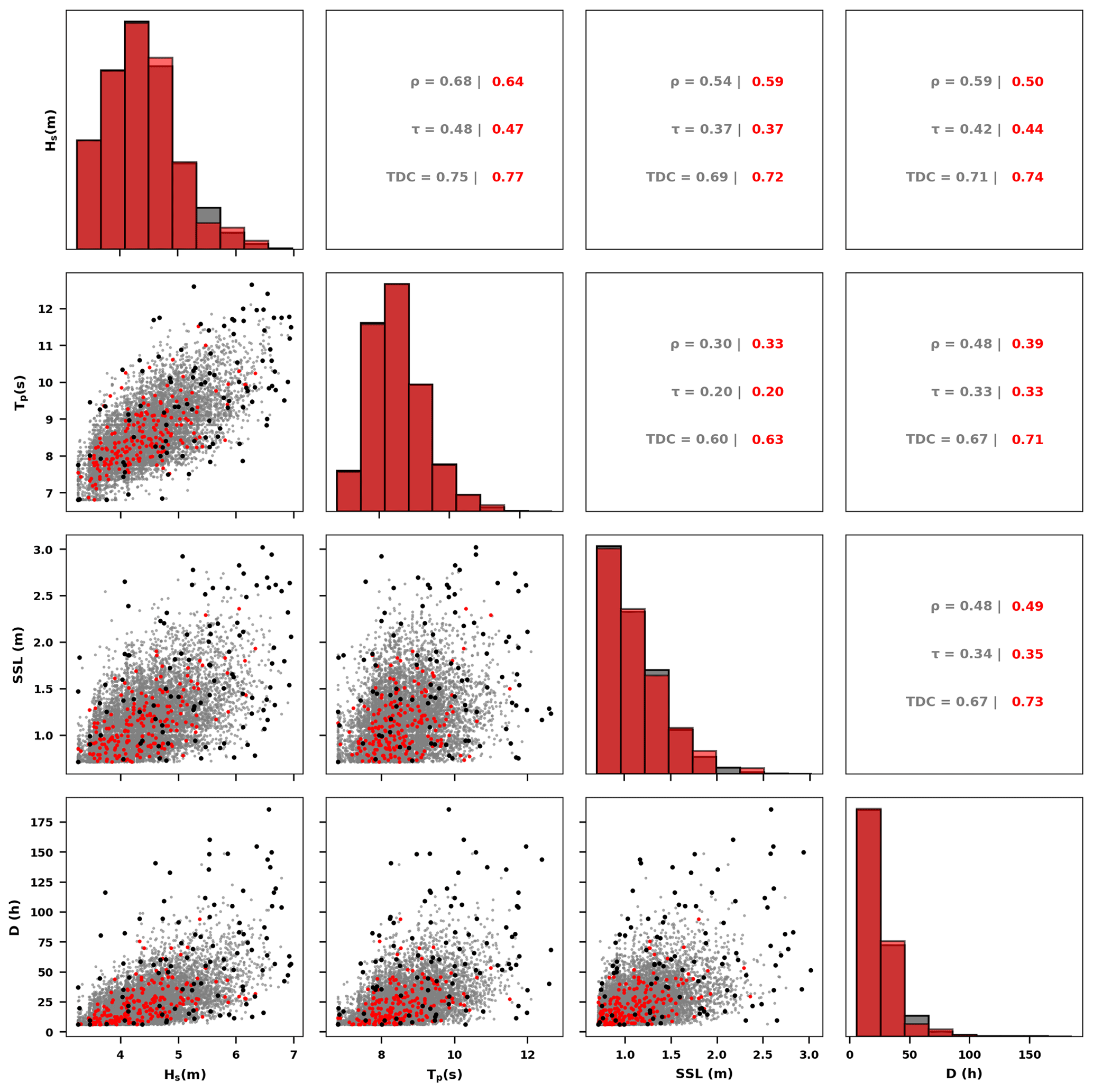
Figure 3 Copula-based events simulator for the Euro platform station location (see Fig. 2). Red, gray and black dots indicate observed, simulated and the 100 MDA selected events, respectively. The black dots are a subset of the gray dots (simulated events) that are selected with the MDA. Histograms of each storm parameter (H_s, T_p, SSL and D) for both observed and simulated events can be seen in the diagonal graphs. Below the diagonal, scatterplots for each pair are plotted. Above the diagonal, three different dependency coefficients (ρ: Pearson correlation, τ: Kendall's rank correlation, TDC: non-parametric tail dependence coefficient) are shown for each pair for the observed and simulated events.

Finally, since we cannot simulate all 100 000 events with our process-based model (Sect. 2.4) due to computational constraints, we used the maximum dissimilarity algorithm (MDA) (Camus et al., 2011; Athanasiou et al., 2021) to sample a representative subset of 100 events (Fig. 3). We preferred to use the MDA relative to other input reduction approaches (e.g., K-means) to ensure that the chosen events were sampling the extreme cases well enough (Santos et al., 2019). Another useful attribute of the MDA is that the most dissimilar cases are picked iteratively, based on their similarity with the rest of the cases. This means that, e.g., the 50 first events from 100 events picked with the MDA will be the same as the 50 events picked with the MDA if a total of 50 samples were chosen. The number of events was chosen to ensure that the subset of events sampled the parameter space sufficiently while keeping the simulation computational costs at a feasible level. This choice was similar to the number of events used in similar studies for the creation of synthetic training cases (Poelhekke et al., 2016; Santos et al., 2019). The copula-based Monte Carlo simulation and the application of the MDA were applied to all four offshore stations (Fig. 2), leading to 100 storm events per area.

2.4 Dune impact synthetic dataset

The process-based model XBeach (Roelvink et al., 2009) was used to simulate the dune response of the 100 TCPs (Sect. 2.2) during the 100 synthetic storm events (Sect. 2.3). XBeach is an open-source, process-based model which simulates shortwave energy and longwave transformation, wave-driven currents, sediment transport, and corresponding morphological changes at sandy coasts. In the present study, the XBeach-v1.24.5867 version was used in a “surfbeat” mode, where the shortwave variations are resolved at the wave group scale. A one-dimensional (1D) cross-shore model was created for each TCP using the topo-bathymetry as extracted from the JARKUS dataset (extended to a 30 m depth assuming a slope of 0.01, to make sure that the offshore boundary was deep enough so that the waves at the boundary are in intermediate water). The cross-shore grid resolution changed from the offshore boundary to the dry beach, reaching a 1 m spacing at the dune area. An extensive calibration of the XBeach settings for use at the Dutch coast was performed in Deltares/Arcadis (2022) using both laboratory experiments and field data (from Belgium, the Netherlands and Germany), resulting in a relative bias of −0.03 and a scatter index of 0.23 for the simulated dune erosion volumes. To reduce the computational time while ensuring minimal influence in computed morphological changes, we used a morphological acceleration factor (morfac) of 5, following Athanasiou et al. (2021).

For each of the 100 TCPs, the 100 synthetic storms derived for the respective offshore wave station (see Fig. 2 and Sect. 2.3) were used to create the XBeach hydrodynamic boundary conditions. The time evolution of the boundary conditions was configured similarly to Athanasiou et al. (2021) using a triangular approach for H_s and T_p and a normalized hydrograph for SSL (derived from the historic events of the respective station), which is rescaled using the individual storm's maximum SSL. The tidal signal was created for each TCP based on observed tidal records and the local MHW, assuming a high tide during the peak of the storm (center of the hydrograph) (Fig. 4a–c). This assumption could give a conservative result with respect to dune erosion. The duration D was used to define the starting and ending time of each simulation. Since the influence of wave obliqueness is not fully resolved in the 1D version of XBeach, here we assumed that the wave direction is shore-normal. This assumption may lead to underestimation of dune erosion when the generation of alongshore currents becomes important for sediment stirring and thus sediment transport (de Winter and Ruessink, 2017). The synthetic wave time series were then used to construct Joint North Sea Wave Observation Project (JONSWAP) spectra time series (γ=3.3 and wave directional spreading of 30^∘) that were imposed at the offshore boundary of the model, together with the superimposition of the SSL and tidal signal.

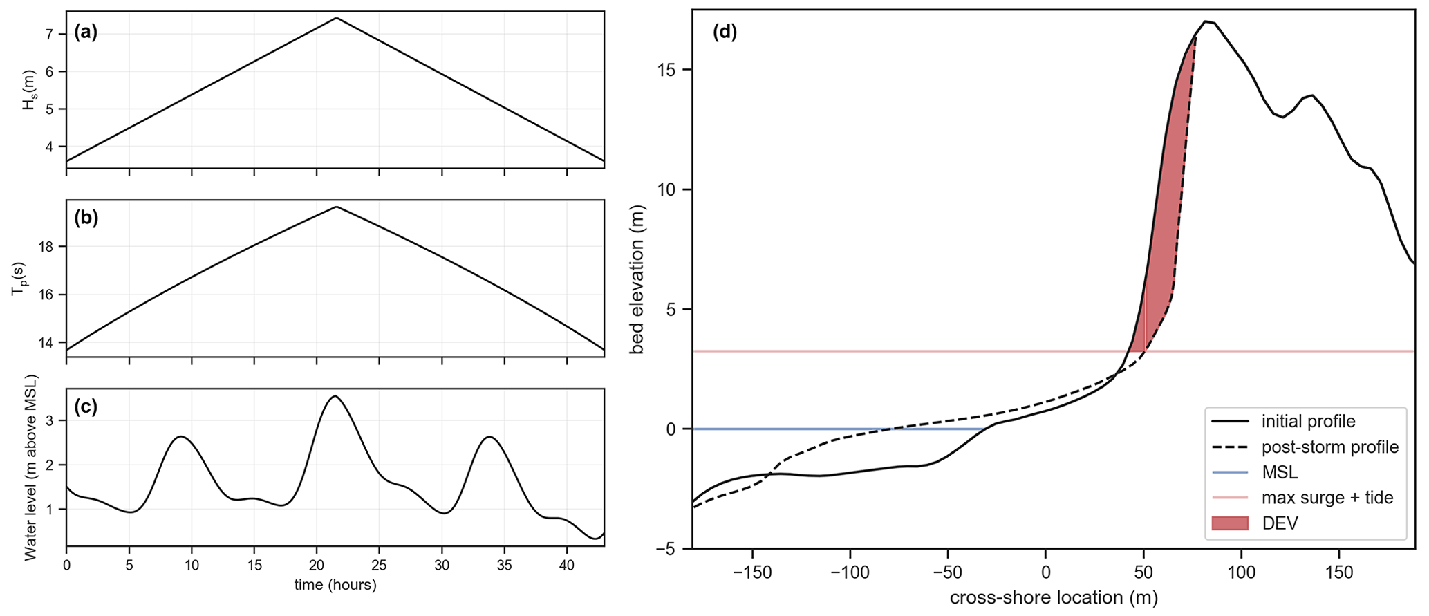
Figure 4 Example of XBeach offshore boundary conditions and dune impact for one selected storm and TCP. (a) H_s time series, (b) T_p time series and (c) water level time series at offshore boundary. (d) Post-storm simulated profile and calculation of dune erosion volume (DEV).

Here, the dune erosion volume (DEV) was chosen as the dune impact indicator (Giardino et al., 2014; Athanasiou et al., 2021) and was calculated for each simulation as the difference of the dune volume per running meter (m³ m⁻¹) above the highest water level during an event, between the pre- and post-storm elevation profiles (Fig. 4d). For the cases were DEV was negative (resulting from storms with relatively small SSL and newly formed dunes fronting the first dune row, leading to onshore sediment transport) or very small (DEV≤0.01, values in this range are not expected to be representative because of grid spacing limitations), the DEV was given a zero value. Additionally, local accretion can be connected with alongshore variability of pre-storm morphology (Cohn et al., 2018; Harley et al., 2022) but cannot be resolved with the 1D approach used in this study.

The synthetic training dataset comprised a total of 10 000 simulations (100 TCPs × 100 storms). Additionally, a synthetic benchmark dataset was created for calibration and validation purposes. This was created by simulating DEV with XBeach for 20 storms, selected using the MDA for each offshore wave station but for a new Monte Carlo simulation (to ensure that the events are different for the ones used in the training dataset) using 127 profiles along the Dutch coast (1 every 10 transects, excluding the TCPs). The previous steps were followed to ensure that the benchmark dataset was independent from the training data but still accounted for the morphological and hydrodynamic variabilities observed at the Dutch coast. In this way, overfitting during model training was avoided while the validation set was still representative enough. The benchmark dataset comprised a total of 2540 simulations (127 profiles × 20 storms).

2.5 Artificial neural network

Artificial neural networks (ANNs) are computational networks that are a subset of machine learning and more specifically deep learning algorithms, inspired by the neuron structure of the human brain. ANNs comprise a series of layers, each one containing fundamental units or nodes of a network. The number of layers of an ANN characterizes the depth, while the number of nodes per layer describes the width of the network. More specifically, multi-layer perceptron feed-forward ANNs include an input layer, one or more hidden layers, and an output layer, with the neurons of each layer being fully connected with the neurons of the previous one and the information passing in a single direction (i.e., from input to output). Thus, each neuron in the hidden and output layers translates the input values that are fed from the neurons of the previous layer to a single output using a set of weights (one for each input neuron), a bias and an activation function. The output y_j of the jth neuron of a layer with m neurons is calculated as follows:

$$\begin{array}{}\text{(1)}& y_j=f\left(\left(\sum _{i=\mathrm{1}}^n{w}_{ij}{x}_i\right)+b_j\right),\text{ with }j=\mathrm{1},\mathrm{2},\mathrm{\dots },m\end{array}$$

where n is the number of neurons in the previous layer, w_ij is the weight of the connection of the ith neuron of the previous layer to the jth neuron of the current layer, b_j is the bias of the jth neuron and f is an activation function.

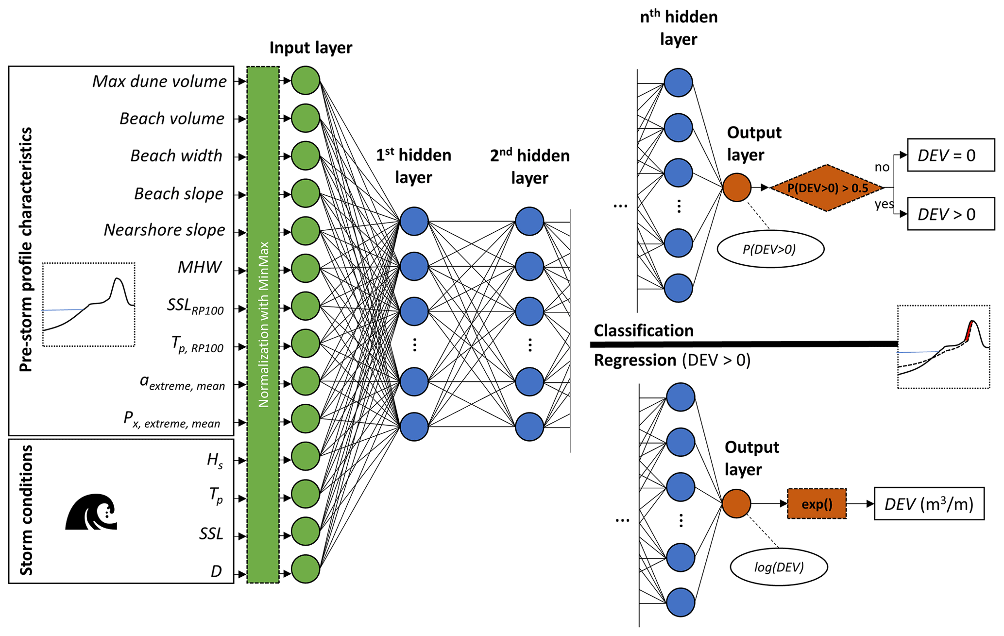
Figure 5 Configuration of the artificial neural network (ANN) for either DEV classification or regression. The first layer (input layer) comprises 14 (10 profile and 4 forcing) parameters, which are normalized. Then, n hidden layers with variable numbers of nodes are defined iteratively, while connections to the nodes of the previous layer are established using weights, biases and an activation function. The last layer is the output layer for which there can be two configurations: (1) classification (upper right), where the output layer comprises one node presenting the probability of DEV >0, which provides an estimate of dune erosion occurrence or not, and (2) regression (lower right), where the output layer comprises one node, which is the log(DEV) that is translated back to its real units using an exponential function.

Here, we built a two-phase ANN for the estimation of DEV, composed of a classification ANN, which first predicts whether there is dune erosion or not, and then a regression ANN, which quantifies the DEV. With this two-phase approach we ensured that overprediction for smaller DEVs was avoided and enabled the prediction of zero DEV (Verhaeghe et al., 2008). For the input layer a total of 14 parameters (neurons) were used (Fig. 5), with 10 parameters describing the characteristics of the pre-storm profile (which are the same parameters used for the clustering procedure in Sect. 2.2) and the 4 storm parameters as defined in Sect. 2.3. To avoid issues in the training of the ANN related to the different scales of the continuous input parameter space, the input data were first normalized to unity range. For both ANNs the initial weights and biases of the neurons in the hidden and output layers were randomly assigned, and then the optimum weights and biases were calculated during an iterative training phase using the standard error backpropagation with the gradient descent method. More specifically, the adaptive moment estimation algorithm (Kingma and Ba, 2017) was used to calculate the optimum weights, by minimizing a loss function between the ANN-estimated DEV values and the target values from the training dataset (the 10 000 cases described in Sect. 2.4).

The benchmark dataset (the 2540 cases described in Sect. 2.4) was equally divided into a calibration and a validation dataset. The former is used for the tuning of the ANN's hyperparameters and comparing the different ANN configurations to choose the optimum one. The latter is used for assessing the actual accuracy and prediction skill of the selected ANN. To avoid overfitting of the model to the training dataset, the learning phase of the ANNs was optimized by using the calibration dataset to stop training when the losses (differences between predictions and targets) for the calibration dataset stop decreasing. Additionally, the hyperparameters of the ANNs, like the batch size (number of samples to work through before updating the internal model parameters), the learning rate (how much to change the model in response to the estimated loss each time the model weights are updated) and the hidden-layer activation functions, were chosen using a grid-search approach identifying the combination minimizing the calibration dataset losses. The division of the benchmark dataset into a calibration and validation dataset was performed 10 times with different randomization seeds, and the final mean error statistics were used, to ensure that any bias of the individual divisions was minimized. This meant that 10 different ANNs were produced (with the same architecture but different weights and biases), which will give an ensemble of DEV predictions that can work as an uncertainty range.

For the neurons in the hidden layer(s) of both the classifying and regression ANNs, the rectified linear (ReL) activation function (Nair and Hinton, 2010) was used:

$$\begin{array}{}\text{(2)}& f\left(x\right)=\max \mathit{\{}\mathrm{0},x\mathit{\}}.\end{array}$$

For the classification ANN, all the cases in the training and benchmark datasets was used. The simulated DEV of all the training and benchmark cases were translated to 0 or 1, representing, respectively, no erosion (DEV=0) or erosion (DEV>0). For the neurons in the output layer the sigmoid activation function was used:

$$\begin{array}{}\text{(3)}& f\left(x\right)={\displaystyle \frac{\mathrm{1}}{\mathrm{1}+e^{-x}}}.\end{array}$$

With this function, the output neuron will always give a value in the range [0, 1], which indicates the probability of having dune erosion and is used to classify the output to “erosion” if it is >0.5 or “no erosion” if it is ≤0.5. Since the problem was a binary-classification one, the loss function used to optimize the classification ANN was the binary cross-entropy (BCE) defined as follows:

$$\begin{array}{}\text{(4)}& \mathrm{\text{BCE}}=-{\displaystyle \frac{\mathrm{1}}{N}}\sum _{i=\mathrm{1}}^N{y}_i\cdot \log \left(p\left(y_i\right)\right)+\left(\mathrm{1}-y_i\right)\cdot \log \left(\mathrm{1}-p\left(y_i\right)\right),\end{array}$$

where N is the number of samples in the training batch; y_i is the actual (observed) class, which is 0 or 1 for no erosion or erosion, respectively; and p(y_i) is the probability of the erosion class as calculated by the ANN.

For the regression ANN only the cases where DEV>0 were used, which comprised 79 % and 77 % of the total cases in the training and benchmark cases, respectively. The DEV values were first transformed to log(DEV) to ensure that during the calculation of losses, similar importance was given to minor and larger DEV cases (van Gent et al., 2007). For the output layer a linear activation function was used, which is defined as f(x)=x, and the final DEV estimation was acquired by using the exponential function on the output neuron to transform them back to real units. Since this problem was a regression one and the natural logarithm of DEV was used as the output, the loss function used in the regression ANN was the mean absolute error (MAE) defined as:

$$\begin{array}{}\text{(5)}& \text{MAE}={\displaystyle \frac{\mathrm{1}}{N}}\sum _{i=\mathrm{1}}^N\left|\log \left({\mathrm{DEV}}_{\mathrm{pred}}\right)-\log \left({\mathrm{DEV}}_{\mathrm{sim}}\right)\right|,\end{array}$$

where N is the number of samples in the training batch, DEV_sim is the dune erosion volume as simulated by XBeach and DEV_pred is the dune erosion volume as calculated by the ANN.

Different architectures of the hidden layers (number of hidden layers and neurons per layer) were tested for both ANNs to find the optimum ones with respect to the calibration dataset. The accuracy metric (i.e., the percentage of correct class predictions) was used to find the optimum architecture of the classification ANN. For the regression ANN, the skill score (Murphy, 1988) was used to choose the optimum architecture, which is defined as follows:

$$\begin{array}{}\text{(6)}& {\displaystyle }\text{skill}=\mathrm{1}-{\displaystyle \frac{{\text{RMSE}}^{\mathrm{2}}}{{\mathit{\sigma }}_{{\mathrm{DEV}}_{\mathrm{sim}}}^{\mathrm{2}}}},\text{(7)}& {\displaystyle }\text{RMSE}=\sqrt{{\displaystyle \frac{{\sum }_{i=\mathrm{1}}^N{\left({\mathrm{DEV}}_{\mathrm{pred}}-{\mathrm{DEV}}_{\mathrm{sim}}\right)}^{\mathrm{2}}}{N}}},\end{array}$$

where ${\mathit{\sigma }}_{{\mathrm{DEV}}_{\mathrm{sim}}}$ is the standard deviation of the XBeach-simulated DEV in the calibration dataset and N is the number of cases in the calibration dataset. A skill score of 1 indicates a perfect prediction. The bias index (BI), RMSE and the modified index of Mielke (λ) (Duveiller et al., 2016; Santos et al., 2019) were also computed as complementary error statistics.

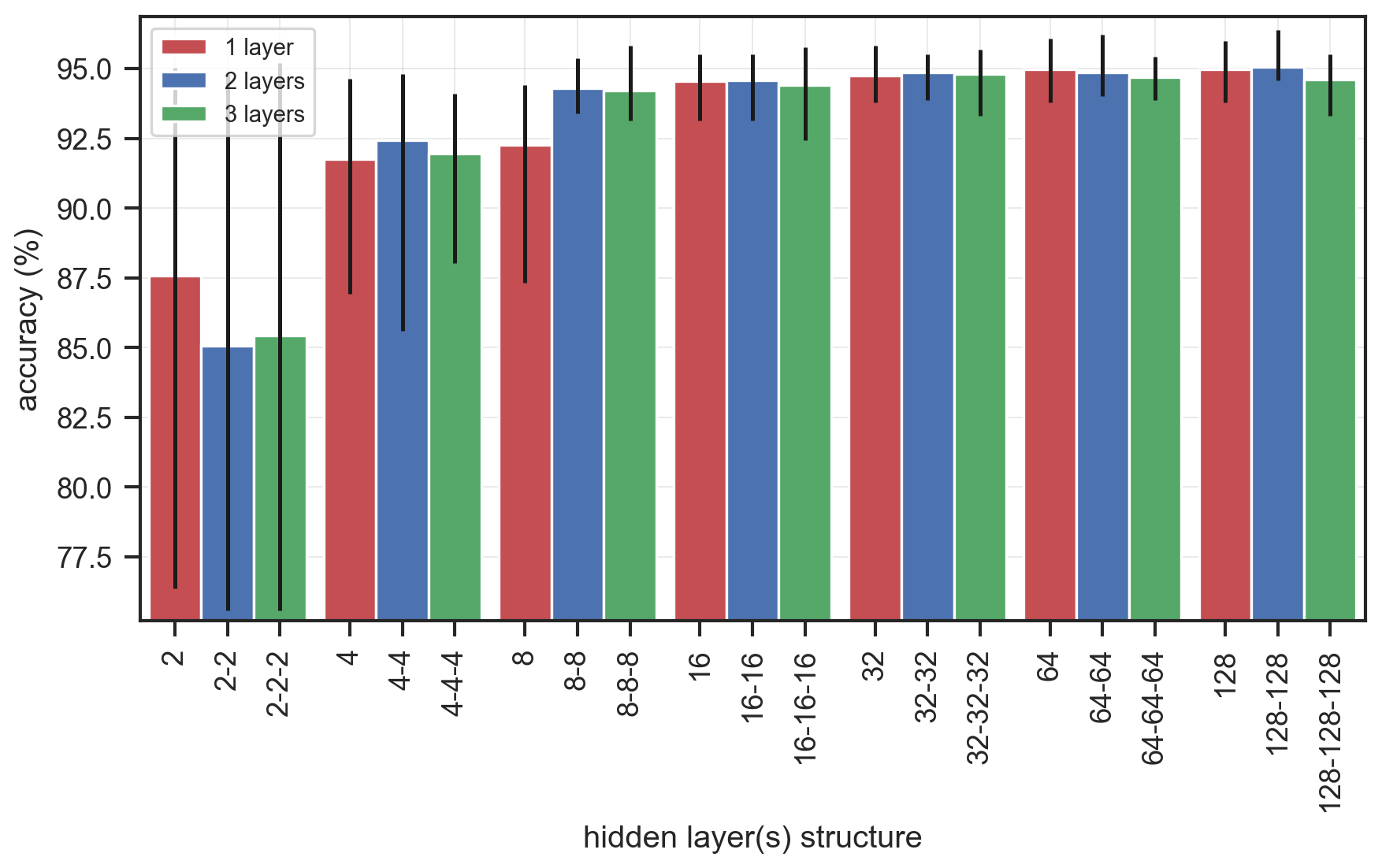
Figure 6 Accuracy of classification prediction for the calibration cases using different architectures of the classification ANN with a different number of hidden layers and neurons per layer. On the x axis the architecture of each ANN is represented by the number of neurons per layer, with layers separated by “–”. The bars indicate the mean accuracy values between the 10 randomizations of the benchmark dataset, and the lines show the min and max values.

3 Results

3.1 Performance of classification ANN

Different depths (number of hidden layers) and widths (number of neurons per layer) of the ANN were tested to find the optimum architecture of the classifier. Architectures with one, two or three hidden layers were tested, with similar numbers of neurons ranging between 2 and 128 (with a quadratic step increase between the tests). The mean accuracy of the predictions for the calibration cases (1270 cases) increased for wider networks, starting from an average accuracy of ∼85 % for a small number of neurons per layer and reaching up to ∼95 % for wider networks (Fig. 6). The difference between networks with one and three hidden layers was negligible, while for networks with more than 16 neurons per hidden layer the relative increase in accuracy was again negligible. This indicated that the accurate binary classification for the prediction of whether dune erosion occurs or not does not necessarily require a complex ANN. Therefore and since the differences between the different architectures beyond a threshold of 16 neurons per layer were in the same order of magnitude as the expected differences of rerunning the algorithm (due to the inherit stochasticity of the training process and the weight initialization), here we opted to use a relatively simple ANN architecture with two hidden layers of 32 neurons each.

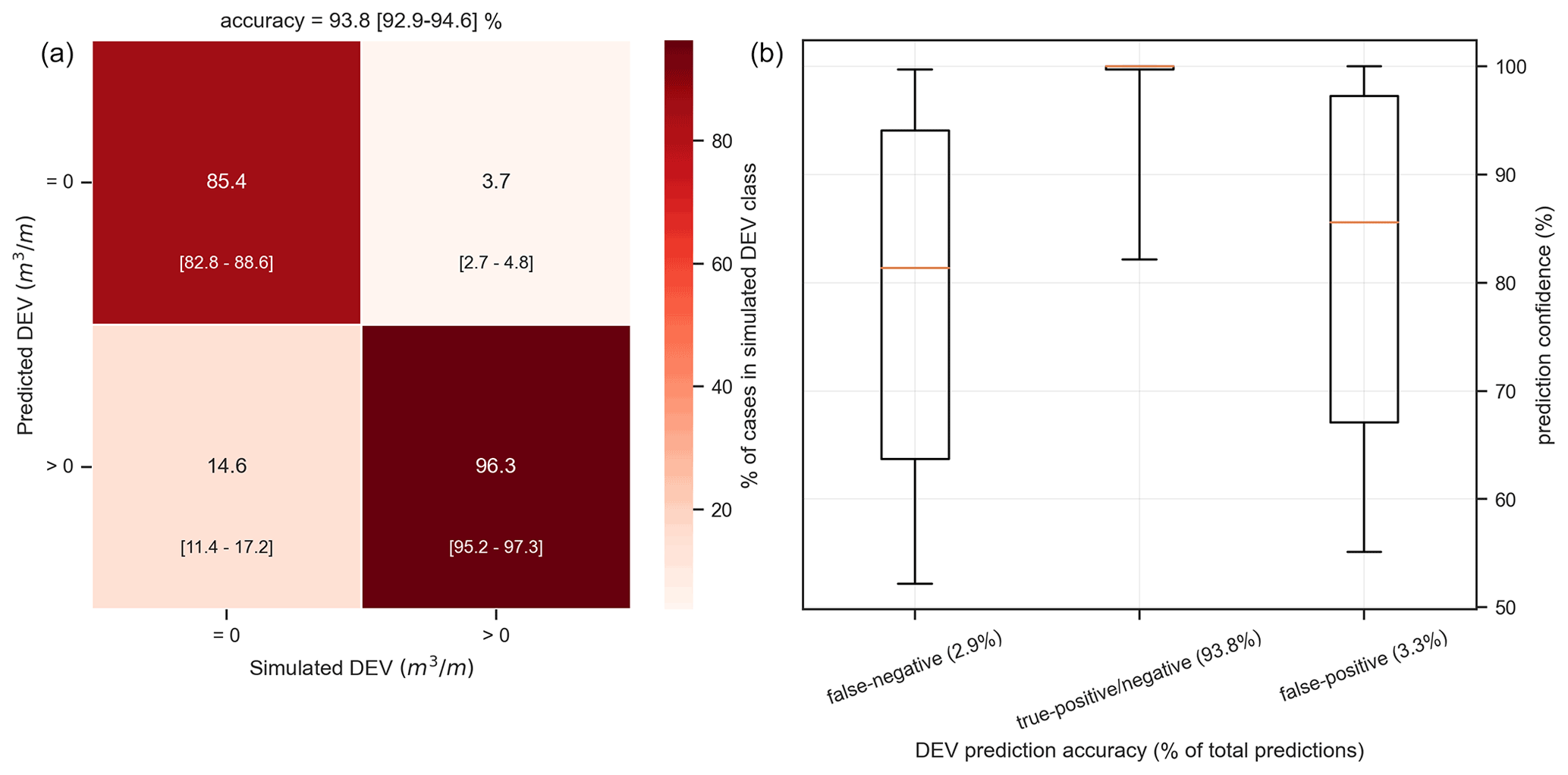
Figure 7 Prediction accuracy of the predicted DEV class using the selected classification ANN configuration (two hidden layers of 32 neurons each) against the XBeach simulated classes for the validation cases. (a) Confusion matrix showing the percentage of each class prediction per observed class (each column sums to 100 %), with the diagonal indicating a correct prediction. Numbers in the center of each cell show the mean accuracy over the 10 randomizations of the benchmark cases, while brackets in the lower part give the min–max values. (b) Boxplots of the prediction confidence (as given by the ANN) grouped by the prediction's accuracy, defined here as the difference between the predicted DEV class and the observed DEV class (orange line: median, box: 25th–75th percentile range, lines: 5th–95th percentile range).

Using the 1270 validation cases the accuracy of the selected ANN was further assessed. The classification ANN predicted the correct class (erosion or no erosion) with an average accuracy of ∼94 %. The confusion matrix shows that the model had an average accuracy of ∼96 % in correctly identifying cases with erosion, while it accurately found ∼85 % of the cases that there is no erosion (Fig. 7). The quite high accuracy in identifying erosion cases provided confidence in the use of this classification ANN as a first filtering step in the proposed meta-model, while the “false positive” cases (∼15 %) are handled in the next phase with the regression ANN, where they can still have a small DEV value. Since the actual output of the classification ANN is the probability of erosion, a prediction confidence can be calculated as the probability of the class with the highest probability. When analyzing the statistics of the prediction confidences (Fig. 7), it can be seen that for accurate predictions (true positive or true negative) the prediction confidence was higher (25th–75th percentiles: 99.7 %–100 %) than that for false negatives (63.7 %–94.1 %) and false positives (67.1 %–97.2 %), indicating that the prediction confidence as given by the ANN is a good measure of the confidence level of the predictions.

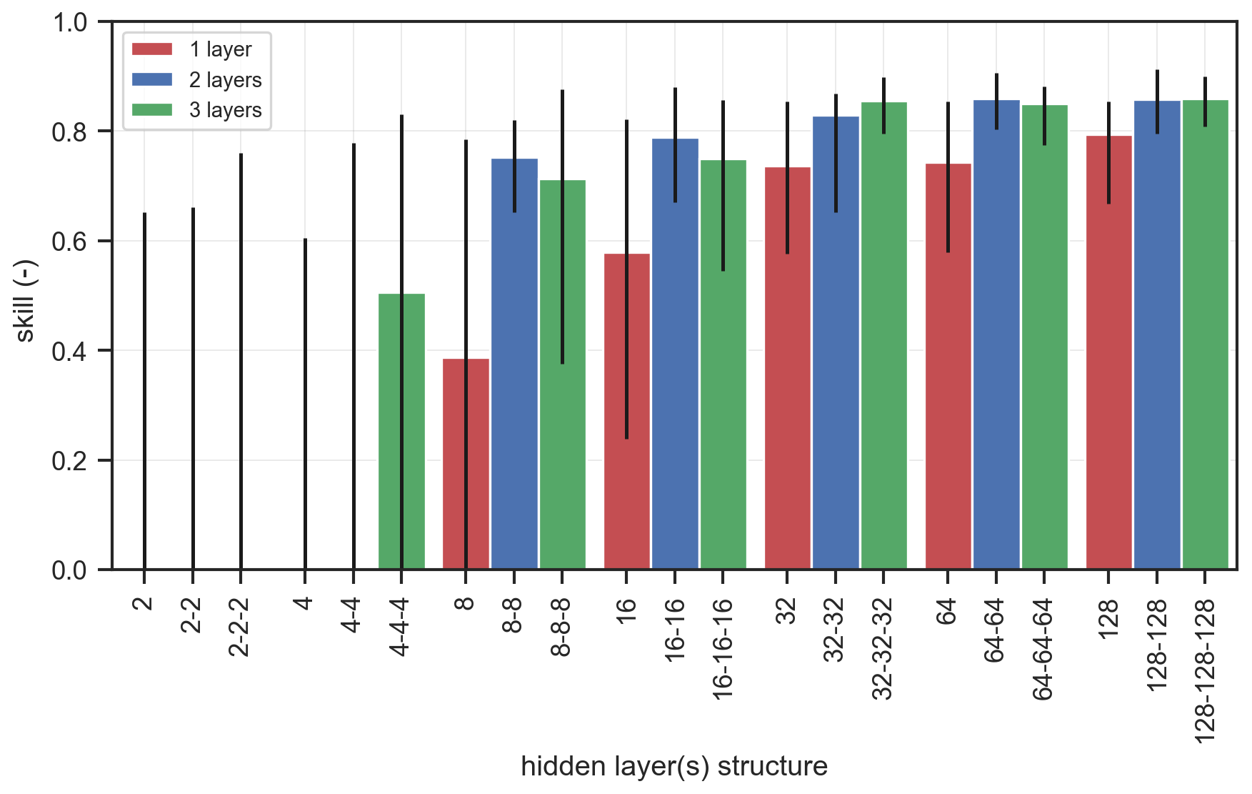
Figure 8 Skill of the DEV prediction for the calibration cases using different configurations of the regression ANN with a different number of hidden layers and nodes per layer. On the x axis the architecture of each ANN is represented by the number of neurons per layer, with layers separated by “–”. The bars indicate the mean values between the 10 randomizations of the benchmark dataset, and the lines show the min and max values. The lower limit of the y axis has been set to 0 to avoid visualization issues when skill was negative for some configurations with low number of layers and nodes.

3.2 Performance of regression ANN

The same architectures as for the classification ANN were tested for the regression ANN. The mean skill score of the predictions for the calibration cases (∼980 cases with DEV >0) strongly increased for wider networks, while the influence of the network's depth was more evident for less wide networks (Fig. 8). The consistency of the skill score between the calibration randomizations (shown by the line around the bars in Fig. 8) increased with wider and deeper networks as well. This indicated that for a skillful prediction of DEV a relatively higher number of neurons (and thus complexity) was needed. Ultimately, a regression ANN with three hidden layers and 32 neurons per layer was selected as the best-performing one.

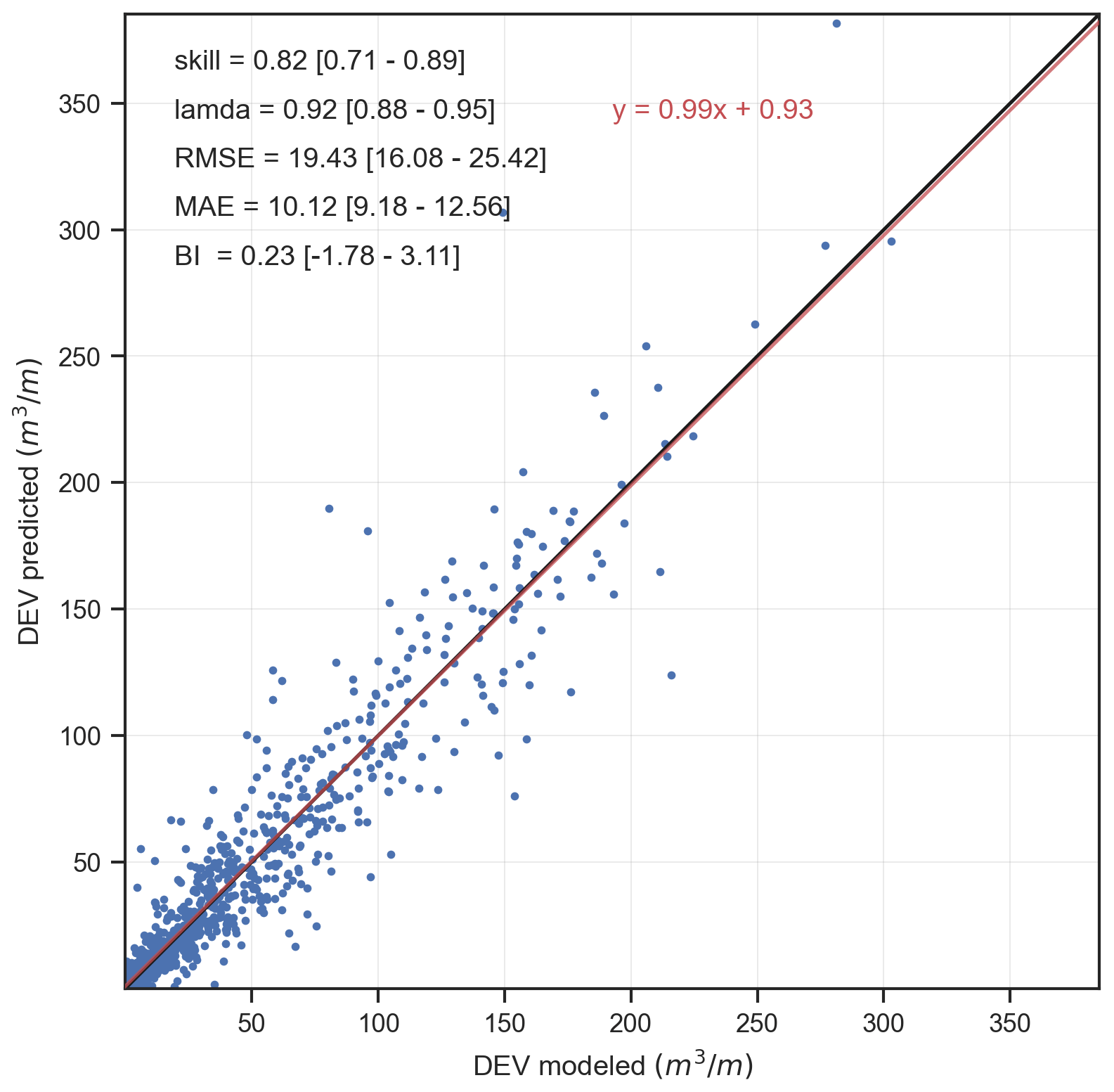
Figure 9 Scatterplot between the XBeach-simulated (x axis) and ANN-predicted (y axis) DEV for the validation cases with DEV >0 m³ m⁻¹ using the selected regression ANN configuration (three hidden layers of 32 neurons each). The scatterplot shows the validation cases for one of the randomizations, while statistics in the upper left show the mean over the 10 randomizations of the benchmark cases, with brackets giving the min–max values. The black line indicates the 1:1 line, while the red line is the linear regression fit (equation given in red).

Using the validation cases (∼980 cases) the error statistics of the DEV predictions with the selected ANN configuration were further assessed (Fig. 9). The ANN-based DEV predictions showed a good agreement with the XBeach-simulated DEVs, with a skill score between 0.71–0.89 (among the 10 randomizations) with an average of 0.82, while the RMSE and the bias had an average value of 19.4 and 0.23 m³ m⁻¹, respectively.

3.3 Comparison with observations

In the JARKUS program, elevation profiles are measured along the Dutch coastline every year around April as described in Sect. 2.1. However, these profiles cannot directly be used as pre- and post-storm profile observations to find dune erosion, since several different events occur and dune recovery occurs between the two measurements.

Table 2 Cases used for the validation of the meta-model predictions.

In this section, we used available pre- and post-storm observations for three historic storms (1953, 1979 and 2019) to validate the prediction capacity of the proposed meta-model against observed DEV. These three storms have been used in the validation of the XBeach model as well (Arcadis/Deltares, 2022). For these storms we extracted the storm conditions using the same methodology as used in the event definition in Sect. 2.3. The storm conditions for three different storms along with a description of the available elevation data are given in Table 2. The input for the ANN-based meta-model was obtained by calculating the morphological indicators of the pre-storm profiles, while the hydrodynamic indicators were obtained from the corresponding transects of interest as calculated in Athanasiou et al. (2021) (see Table 1).

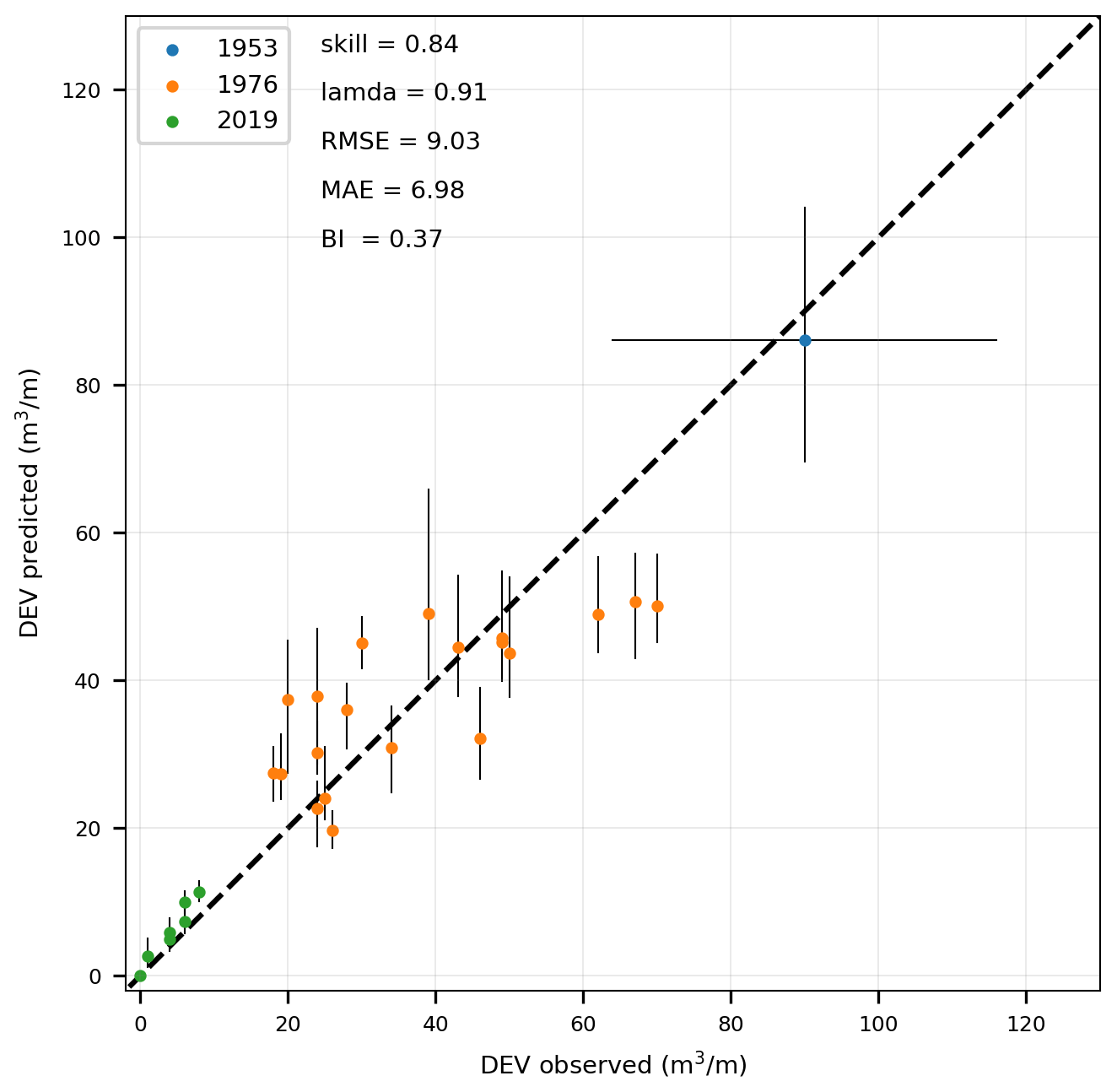
Figure 10 Scatterplot between the observed (x axis) and ANN-predicted (y axis) DEV for three historic storms with a variable number of transects per storm. The dots indicate the average predictions of the ANN, while the vertical lines show the min and max values as given by the ensemble of the ANN output. For the storm of 1953 the horizontal line gives the range of the values reported.

A scatterplot of the observed versus the ANN-predicted DEV for the different storms and transects (Fig. 10) reveals that the variability in DEV values between the three storms was modeled well. For the moderate-intensity storm of 2019, the variability between the different measured transects was captured accurately. However, for the case of the 1976 storm there was some underestimation for the transects with observed DEV >40 m³ m⁻¹ and some overestimation for the transects with DEV <40 m³ m⁻¹. This might be an artifact of the way the pre- and post-storm profiles were created in that the 1976 storm observations only included the part up to the dune toe. For that reason, part of these discrepancies can be attributed to the quality of the measured data. For the disastrous event of 1953, the mean DEV prediction was in the range of the reported DEV values. Using these 38 cases, error statistics were computed for the mean DEV prediction of the ANN-based meta-model. The DEV predictions had a skill score of 0.84 and RMSE of 9.15 m³ m⁻¹ against the 38 observed DEVs. The error statistics against the observed cases (Fig. 10) are comparable to the ones derived against the benchmark cases (Fig. 9), with the exception of the RMSE, which is almost half the size. This is due to the relatively smaller scale of observed DEV in comparison to the simulated DEV in the benchmark dataset.

4 Discussion

4.1 Insights

During the creation of the ANN-based meta-model, a specific set of profile and storm parameters was used as input features for the DEV predictions (Fig. 5). The 10 profile parameters used herein were the same ones used in the clustering procedure as presented in Athanasiou et al. (2021), which were found to drive DEV variability during storms at the Dutch coast. During the clustering procedure (Sect. 2.2), specific weights were assigned to each of these 10 parameters according to their importance (Table 1). These weights, however, were not used in the ANN creation because a weighting scheme is implicitly taking place during the training of the ANN when weights are assigned to each incoming connection of each individual neuron. Since there are numerous connections and different layers, it is not straightforward to get individual weights for each of the input parameters of the trained ANN as a measure of input importance. Still, there are techniques that allow for assessing the individual impact of inputs in an ANN (Wang et al., 2000).

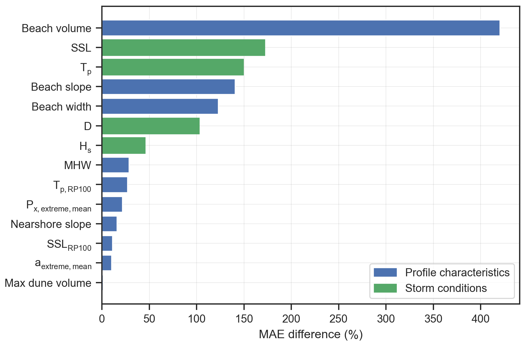
Figure 11 Input parameter importance using a permutation importance approach. The bars indicate the mean MAE difference between the MAE when permutating a single-input parameter and the MAE of the benchmark cases with no permutations.

Here we employed a permutation importance approach (Breiman, 2001; Logue et al., 2019) to assess the individual importance of the input parameters in predicting DEV using the ANN framework. To this end, the trained regression ANN was used to predict DEV for the validation cases after each feature (i.e., input parameter) was first randomly permuted one at a time. Then, the MAE was calculated for each permutation and compared with the benchmark MAE (using the validation cases without permutations) (Fig. 11). The underlying idea is that if an input feature is important, then shuffling its values will lead to larger errors in the predictions. The pre-storm beach volume was found to be the most important input in predicting DEV. The other beach characteristics (width and slope) were important as well, highlighting that the beach fronting the dune acts as a first buffer protecting the dune from erosion. The storm's SSL, T_p and D were found to be quite important inputs as well (in that order). These results agree with Beuzen et al. (2019), who found beach width and the exceedance of wave run-up above the dune toe as the most important drivers of observed dune erosion variability during a single storm along the southeast Australian coastline. The max dune volume was found to be the least important input for the DEV predictions, which agrees with Athanasiou et al. (2021). It should be noted, though, that some of the parameters that are expected to be important, e.g., the storm's H_s, did not lead to a high MAE difference, something that could be connected with their correlation to other more important parameters (see Fig. 3) that mask part of the individual importance during the permutations.

One of the most critical aspects when training machine learning models, like the ANN presented here, is the training dataset. The predictive capacity of the ANN is highly dependent on how well the training cases sample the parameter space, allowing for generalization of the model and avoiding overfitting. To ensure a representative (for the Dutch coast) training dataset, here 100 elevation profiles (TCPs) were chosen based on a clustering analysis of all the available transects at the Dutch coast (Athanasiou et al., 2021), while for the storms, a total of 100 storms was selected based on previous studies and available computational power. However, since for the selection of storm events the MDA was used, which does not randomly pick events from the storm parameter space but rather incrementally includes the most dissimilar events in the chosen subset (i.e., the order the events are picked is always the same); there is a chance that not all of the 100 events used here were needed to capture the variability of the synthetic storms produced in Sect. 2.3. To test this, we trained the regression ANN with a different number of cases representing the combination of the 100 TCPs with a different number of events as given by the MDA (5, 10, 20, 50 and 100 storm events) and validated the prediction skill of each ANN (Fig. 12). The prediction skill reached a plateau after 20–50 storm events were used. This means that with around 20–50 events, the MDA has already picked the most dissimilar events.

Figure 12 Skill value for a different number of training storm events used from the MDA (5, 10, 20, 50 and 100). The thick line shows the mean values while the patch indicates the min and max values between the 10 randomizations of the validation dataset. The patch extents have been smoothed using a Gaussian smoother.

In our study, running 10 000 XBeach simulations for the training dataset was feasible using parallel computing. However, as shown in Fig. 12, more than half of these simulations were actually not necessary to attain the predictive skill that was demonstrated in Sect. 3.2. To this end, this “spare” computational effort for creating a synthetic training dataset could be devoted to adding complexity to the meta-model by reducing some of the assumptions used in the presented framework. For example, 2D XBeach models could be used instead of 1D, enabling the simulation of oblique waves during storms by adding the wave direction as an extra input parameter in the ANN. Additionally, the assumptions with respect to the time evolution of the water levels and wave conditions during a storm used here (see Sect. 2.4) could be replaced by expanding the simulations with different H_s and SSL hydrographs and different phasing between the peak of SSL with the high tide. The effects of the aforementioned assumptions are further discussed in the next subsection.

4.2 Limitations

Machine learning models based on supervised learning, like the presented ANN-based meta-model, are as good as the data used to train them. Due to lack of a sufficiently large number of post-storm dune erosion observations at the Dutch coast, the training dataset used here was a synthetic dataset created using a calibrated version of the process-based model XBeach, which has shown good skill in predicting dune erosion at the Dutch Coast (Arcadis/Deltares, 2022) and has been previously used in numerous studies showing good skill in reproducing dune erosion during storms (Lindemer et al., 2010; McCall et al., 2010; Vousdoukas et al., 2011; de Winter et al., 2015; Passeri et al., 2018). Still, due to the computational burden of creating the synthetic cases, specific assumptions and simplifications needed to be followed, which can affect the predicting capacity of the presented meta-model.

One of the main simplifications was using a 1D model and assuming that waves are shore-normal. This was decided due to the high computational cost of running ∼10 000 2D-XBeach models, which can handle the incoming wave obliqueness. Nevertheless, storms are not everywhere shore-normally incident along the Dutch coast and alongshore non-uniformity and incoming wave angle can affect the dune erosion intensity due to generation of alongshore currents and sediment transport gradients (de Winter and Ruessink, 2017). Additionally, since with the copula-based approach used here (Sect. 2.3) we could only simulate the main storm parameters (H_s, T_p, SSL and D), the time evolution of the wave characteristics and water levels used in the XBeach boundary conditions needed to be schematized. Here we used a triangular hydrograph for the time evolution of the significant wave height and a representative normalized hydrograph based on historic events for the time evolution of storm surge while it was assumed that the high tide always occurs at the same time as the surge peak. While these choices were based on a previous study showing good agreement with observed parameters that can drive dune erosion (Athanasiou et al., 2021), these assumptions have been previously found to introduce extra uncertainties into the modeling of dune impacts (Duo et al., 2020). Some of these assumptions might explain some of the differences between the predicted and observed DEV for the historic cases (Fig. 10).

The choice of the profile and storm parameters used as input in the ANN was based on previous studies looking into drivers of dune erosion variability (Beuzen et al., 2019; Cohn et al., 2019; Athanasiou et al., 2021). However, there are other variables that can be of importance at other dune-fronted coastlines around the world. For example, sediment grain size effects were not taken into account in the present study, since the D₅₀ variability at the Dutch coast is not high enough and is not expected to drive strong differences in DEV variability (Athanasiou et al., 2021). Additionally, vegetation characteristics can play an important role in controlling dune erosion intensity during extreme events (Charbonneau et al., 2017) and were not studied here. In the presented meta-model, the nearshore area of the profile was only described by the nearshore slope. However, pre-storm bar morphology is of importance for post-storm dune erosion (Castelle et al., 2015). Moreover, since the training data of the ANN comprise a set of parameters that are defined in a quite specific manner (see Table 1), it is critical to follow the exact same definition when making predictions, since the model is data-driven rather than process-driven.

The width and height of the dunes along the Dutch coast result in the former being in the collision regime (Sallenger, 2000) during storms, and overwash or inundation is extremely rare. The dune response indicator used in the present study was the dune erosion volume, which is a good indicator to characterize the scale of erosion during extreme storms and provides useful information in long-term planning of nourishment strategies (Giardino et al., 2014). However, several flooding or erosion indicators can be of relevance for other applications or locations (Leaman et al., 2021), such as dune retreat or dune crest lowering (Santos et al., 2019). The presented techniques could be expanded for these impact indicators.

4.3 Applications

The proposed meta-model could have various applications in coastal zone management due to its accuracy and efficiency in generating output. A prediction of DEV for all sandy transects of the Dutch coast when a forecast of an incoming storm is available takes a matter of seconds using this model. This highlights its potential use in an early warning system when compared to the computational power needed when running XBeach for all transects, leading to 10³–10⁴ times faster computations depending on the storm's duration. A hybrid approach could be followed as well, where the ANN meta-model could be used as a screening tool to identify hotspots of dune erosion, reducing the number of XBeach model runs needed to only the locations that are expected to have higher impacts.

Another potential application could be in dune erosion risk assessments, where the meta-model could be applied to quickly quantify DEV along the Dutch coast for all historic storms observed from the offshore stations. Then with extreme value analysis at each transect, local extreme values of DEV could be derived which can aid in assessing local coastal protection. Moreover, if the presented framework is expanded to predict dune retreat and include sea level rise, it could be used for sea-level-rise-induced coastal retreat assessments as well using the Probabilistic Coastal Recession (PCR) tool (Ranasinghe et al., 2012). By efficiently picking the storm boundary conditions to model for the creation of the training data (Fig. 12), extra computational power will be available to include sea level rise (SLR) scenarios. For example, with 100 TCPs, 20 synthetic storms per TCP and 5 SLR scenarios (e.g., 0.2, 0.4, 0.6, 0.8, 1), a total of 10 000 simulations will be needed. The SLR could directly be imposed in the offshore boundary of the new XBeach runs. Then a similar ANN-based meta-model could be trained with the extra input parameter of SLR and having dune retreat as output. The PCR tool has been previously applied to one location at the Dutch coast (Li et al., 2014b) using an empirical relationship to estimate dune retreat during extremes. This probabilistic model requires a quite high number of simulations of coastal retreat, something that could be easily handled with the meta-model approach presented here.

The presented framework could be also expanded to enable the assessment of nourishment strategies. As mentioned in the previous section, the predictive capacity of an ANN is dependent on the training data. This means that elevation profiles with a sand nourishment might not look like any of the TCPs used in the training dataset. To address this, schematic profiles with various nourishment options could be created, then simulated with XBeach and finally added to the training cases. This will allow for more versatility in the predictive capacity and application range of the technique.

Finally, the ANN-based meta-model presented here is tailored to the Dutch coast, and applying it anywhere else in the world would not be straightforward (except where the elevation profiles and forcing look similar). Particularly, the training data used here to develop the meta-model were specific for the Dutch coastal setting with respect to coastal morphology and storm conditions. This means that the predictive capacity of the meta-model is dictated by the training data coverage of the input parameter space. However, the methodological framework (Fig. 1) could be upscaled by creating a new training dataset, which would be based on XBeach simulations of a larger set of profiles that are representative of the global range of beach–dune morphologies and forcing conditions. When doing so, care should be taken to potentially introduce other critical input parameters, which can vary globally, like the sediment grain size. Additionally, special care should be taken in applying these methods in tropical-storm-prone areas, where it should be ensured that the training forcing conditions are representative of the extremes induced by tropical cyclones (Bloemendaal et al., 2022). A meta-model like this could be used as a fast screening tool for dune erosion estimation at any study site with dunes around the globe, especially at data-poor locations. However, availability of dune erosion data will remain a limiting factor for validating the model.

5 Conclusions

A meta-model based on artificial neural networks (ANNs) and the process-based model XBeach has been developed to derive estimates of dune erosion volume (DEV) at the Dutch coast. The model can provide DEV predictions for the entire Dutch coast in a matter of seconds when compared to brute-force modeling with XBeach. The first step of this two-phase model was to predict whether dune erosion occurs or not using a classifying ANN which showed a mean accuracy of 94 % against a benchmark dataset created with XBeach simulations. The second step comprised a regression ANN which estimated DEV with a mean prediction skill of 0.82 and RMSE of 19.4 m³ m⁻¹ against the benchmark data. Additionally, the predictive capacity was tested against some sparse observations of dune erosion for three historic storms at the Dutch coast, showing similarly good performance.

Input reduction techniques were used to ensure that the training data used for the ANNs included representative combinations of elevation profiles and storm conditions. The input parameters of the meta-model included local morphological and hydrodynamic parameters as well as a set of storm-specific forcing conditions. Moreover, various ANN architectures were tested to find the optimum classification and regression ANNs. Using an input importance analysis, the local beach geometry, storm surge level, peak wave period and duration of the storm were found to be the most important inputs for more accurately predicting DEV. Potential applications of the presented model include early warning systems and probabilistic risk assessments of dune erosion, while the methodology could potentially be upscaled using more data from other beach and dune coasts around the world.