the Creative Commons Attribution 4.0 License.
the Creative Commons Attribution 4.0 License.
 | 20 Oct 2022
Development of black ice prediction model using GIS-based multi-sensor model validation
Seok Bum Hong
Hong Sik Yun
Sang Guk Yum
Seung Yeop Ryu
In Seong Jeong
Fog, freezing rain, and snow (melt) quickly condense on road surfaces, forming black ice that is difficult to identify and causes major accidents on highways. As a countermeasure to prevent icing car accidents, it is necessary to predict the amount and location of black ice. This study advanced previous models through machine learning and multi-sensor-verified results. Using spatial (hill shade, river system, bridge, and highway) and meteorological (air temperature, cloudiness, vapour pressure, wind speed, precipitation, snow cover, specific heat, latent heat, and solar radiation energy) data from the study area (Suncheon–Wanju Highway in Gurye-gun, Jeollanam-do, South Korea), the amount and location of black ice were modelled based on system dynamics to predict black ice and then simulated with a geographic information system in units of square metres. The intermediate factors calculated as input factors were road temperature and road moisture, modelled using a deep neural network (DNN) and numerical methods. Considering the results of the DNN, the root mean square error was improved by 148.6 % and reliability by 11.43 % compared to a previous study (linear regression). Based on the model results, multiple sensors were buried at four selected points in the study area. The model was compared with sensor data and verified with the upper-tailed test (with a significance level of 0.05) and fast Fourier transform (freezing does not occur when frequency = 0.00001 Hz). Results of the verified simulation can provide valuable data for government agencies like road traffic authorities to prevent traffic accidents caused by black ice.
- Article
(11892 KB) - Full-text XML
- BibTeX
- EndNote


Meteorological conditions such as fog, freezing rain, and snow (melted and refrozen) lead to the formation of black ice in dark and cold places, such as bridges, tunnel entrances, and shady roads. Black ice is a thin coat of ice on black asphalt, making it difficult for drivers to visually distinguish it from public roads (Cary, 2010). Black ice can cause significant traffic accidents because it occurs rapidly in weather conditions such as freezing rain (Kämäräinen et al., 2017). Over the past 5 years, the number of fatalities in traffic accidents due to black ice is 4 times that of fatalities caused by snow (Traffic accident article (case1), 2022a). In winter, the fatality rate is higher than during periods with general road conditions. Therefore, it is essential to devise measures to prevent ice-related traffic accidents in many mountainous and shady areas, such as the city of Suncheon in Korea. Research is needed to predict and verify the amount and location of black ice using modelling as a basis for establishing countermeasures.
This study predicts the amount and location of black ice by modelling winter ice on a Korean mountainous highway in winter, expressed as a simulation using the geographic information system (GIS). Subsequently, the model was verified using a multi-sensor. Korea has four distinct seasons, and in winter, the temperature drops to a minimum of −10 ∘C (An and Choi, 2013). In addition, Korea is surrounded by sea on three sides, and various types of inland water bodies such as lakes, rivers, and mountainous regions are evenly distributed, thus facilitating formation of black ice (Cary, 2010). Various types of icing traffic accidents occur annually, depending on the environment prone to black ice (Traffic Accident Analysis System, 2017). On 3 December 2021, nine ice accidents occurred in Chungbuk, Korea, from 05:00 to 11:00 LT. At 07:38 LT, seven vehicles collided on the road in Saenggeuk-myeon, Eumseong-gun, and Chungcheongbuk-do, injuring two people. At 20:30 LT, 1 t trucks hit each other in Chilseong-myeon, Goesan-gun, and Chungcheongbuk-do, and one person was injured (Traffic accident article (case2), 2022b). On the morning of 6 January 2020, 41 vehicles collided on National Highway 33 in Gyeongsangnam-do, wounding 10 people (Traffic accident article (case3), 2020). On 14 December 2019, a chain collision occurred on the Sangju–Yeongcheon Highway due to black ice, killing 7 people and injuring 42 others (Traffic accident article (case4), 2019a). On the morning of 15 November 2019, black ice caused a chain collision of 20 vehicles, resulting in significant damage (Traffic accident article (case5), 2019b). Analysis of these cases revealed an average of −1.9 ∘C to be the lowest temperature on the days of the incidents, and the average cloud cover was 5.6 (maximum 10). The average daily precipitation was 4.3 mm, and the average sunrise time was 07:28 LT. The average accident time was 07:05 LT (KMA, 2018). Traffic accidents usually occur in the morning around the time of sunrise, when there is precipitation on average, and the minimum temperature is below 0 ∘C.
Various studies have been conducted on black ice, and the cause of its occurrence has been elucidated to some extent. There are multiple causes, such as freezing of moisture formed due to fog on road surfaces, rainwater from during the day that is subsequently frozen at night, rapid freezing of freezing rain, and refreezing of melted snow (Cary, 2010). Among them, the cause of high fatality is “freezing rain”, i.e. extremely cooled rain that does not have enough time to freeze below 0 ∘C before it hits the ground/road surface and then freezes rapidly at the moment of impact (Cheng et al., 2007). As freezing rain freezes as soon as it hits the road, it is difficult to intuitively predict the amount and location of black ice (Hull, 1999). Therefore, it is essential to select a vulnerable section where black ice is expected based on fog (moisture), freezing rain, and snow (melt) and prevent icing traffic accidents through structural or non-structural measures.
Modelling the amount and location of black ice and a GIS simulation process based on this is required to select sections vulnerable to freezing traffic accidents. Black ice modelling for GIS simulation was performed based on system dynamics, a method of simulating dynamic phenomena by connecting the causal relationships of factors in the form of a block diagram (Kim, 2021; Forrester, 1994). Road freezing is difficult to predict with human intuition, as it occurs due to the time series relationship of factors; thus, system dynamics are more suitable for modelling this phenomenon (Terzi et al., 2021). The GIS is a tool for simulating system dynamics and conducting research on various disasters. Studies using the GIS include ice and snow analysis (Jeong et al., 2019; Koumoutsaris, 2019; Bardou and Delaloye, 2004; Cheng et al., 2007), flood analysis (Wang et al., 2021), underwater volcanic eruption modelling (Hayward et al., 2022), traffic analysis during natural disasters (Toma-Danila et al., 2020), and earthquake and landslide analysis (Yi et al., 2019; Ali et al., 2019), among others. In this study, as well as in predicting and mapping (simulation) black ice, the GIS was applied by referring to previous disaster-related studies. The GIS dynamics modelling study was based on spatial and meteorological data. In this study, we used digital elevation models, hill shade, roads, bridges, river systems, and lakes as spatial data and air temperature, cloudiness, vapour pressure, precipitation, wind speed, snow (melted), specific heat, latent heat, and solar radiation energy as meteorological data. Prior to starting a full-scale study using major factors, previous studies on related topics were analysed to explore the justification of black ice modelling and validation studies. The representative studies are as follows.
Kangas et al. (2015) performed numerical modelling of factors related to black ice. They predicted road surface conditions and traffic conditions using the numerical weather prediction (NWP) model. However, the prediction of the location and the generated amount of road icing is insufficient, and the model lacks validation (Kangas et al., 2015).
Bezrukova et al. (2006) performed numerical modelling to predict the occurrence of black ice. They developed a block diagram model to estimate the ice index based on road surface temperature, air temperature, and humidity. Their model could predict the occurrence of black ice at a superficial level. However, the prediction of the location and amount of black ice was insufficient, and the model was not validated (Bezrukova et al., 2006).
Chapman et al. (2001) estimated road temperature through numerical modelling. They analysed the relationship between road temperature and latitude, altitude, sky-view factor, screening, roughness length, road construction, traffic density, and topography. However, the prediction of the amount and location of black ice is insufficient, and the model was not validated (Chapman et al., 2001).
Lee et al. (2018) performed numerical modelling related to the black ice on Jeju Island, the southernmost island in Korea. Although the air temperature and wind speed were predicted using the Weather Research and Forecasting (WRF) model, the prediction of road icing was insufficient, and the model was not validated (Lee et al., 2018).
Table 1Developments of this study compared to previous studies.
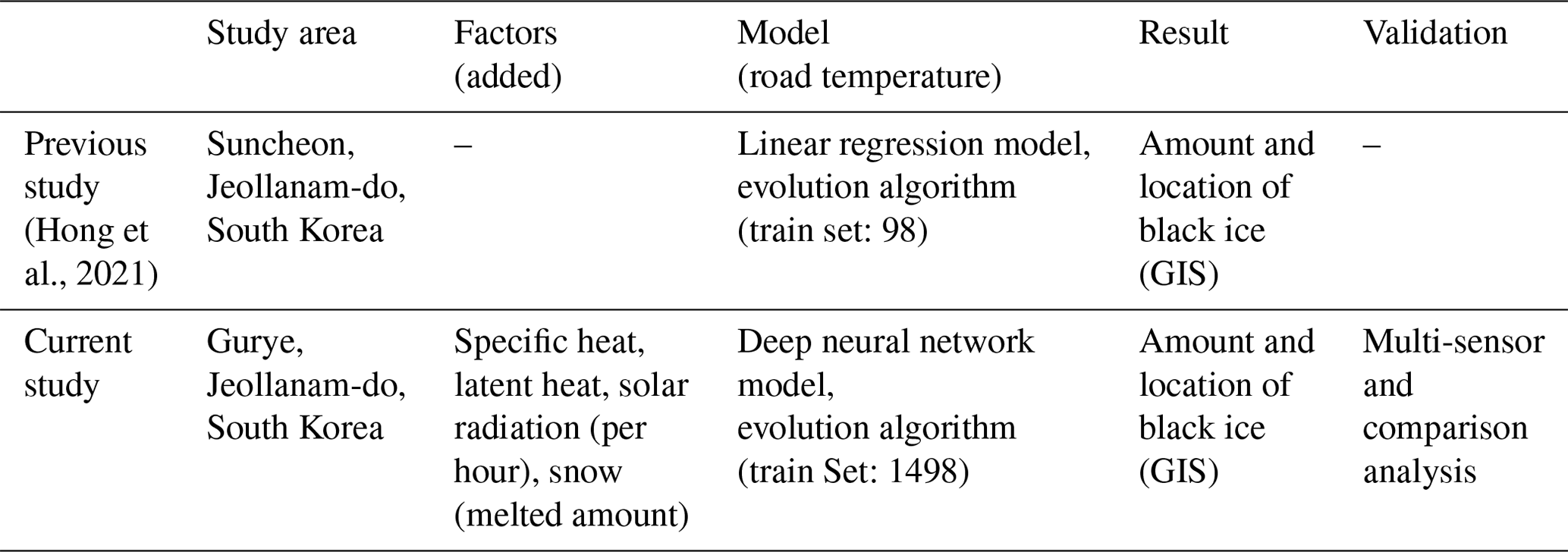
Hong et al. (2021) estimated the amount and location of black ice based on system dynamics and simulated the results using the GIS. The linear regression analysis, the most basic statistical analysis technique, was used for road temperature prediction, and black-ice-related factors are relatively simple. However, the black ice prediction model has not yet been validated (Hong et al., 2021).
Liu et al. (2017) proposed sensor-based GIS visualisation technology for black ice management. The traffic danger section was visualised by interpolating sensor information using overlapping spatial data, such as roads, on the GIS. In addition, a methodology for determining whether black ice is generated by the fusion of an ice sensor based on electrical conductivity and temperature information has been presented. Although the sensor monitoring technique has been efficiently proposed, the modelling part is insufficient, and the sensor configuration is simple (Liu et al., 2017).
In another study, simple numerical modelling was used to predict black ice. Related studies include road temperature prediction using the integrated model of the Korea Meteorological Administration (KMA) (Park et al., 2014), heat conduction analysis due to air temperature and humidity of road surface (Sass, 1992), salinity and temperature measurement and analysis of road surface (Xu et al., 2017), and development of a black ice estimation algorithm for sensors (Troiano et al., 2010; Teke and Duran, 2019). As in previous studies, the estimation of the amount and location of black ice was insufficient, and there was no model validation.
Using these methods, factors related to black ice can be systematically predicted. However, in many studies, the combination of spatial and meteorological data is insufficient, and the simulation step for the location of occurrence has been omitted. In addition, most studies have not performed model validation using sensors. Incorporating the amount and location prediction step in the numerical modelling of black ice improves its efficiency and aids in preparing for traffic accidents in winter, going beyond simple road temperature prediction (Chapman et al., 2001). A previous study of system dynamics modelling for estimating the locations of road icing using the GIS by Hong et al. (2021) predicted the occurrence and location of black ice (road icing) using both meteorological and spatial data, which was simulated using the GIS (Hong et al., 2021). However, because the previous study predicted road temperature, the most critical factor in black ice prediction, using a relatively simple statistical analysis technique of linear regression, it is necessary to improve the prediction accuracy using a more advanced technique. In addition, consideration of black-ice-related factors, such as specific heat, latent heat, solar radiation energy (per hour), and snow (melt), is insufficient, and additional modelling of these factors is required (Liu et al., 2021). Moreover, as in other cases, the validation of the model is insufficient. Compared with previous studies (Hong et al., 2021), the areas developed in this study are shown in Table 1. In this study, Gurye, Jeollanam-do, with a more significant proportion of mountainous regions than Suncheon, Jeollanam-do, was selected as the study area. The added factors are specific heat, latent heat, solar radiation energy (per hour), snow (melting), etc. Through the added factors, the phenomenon of water generation at temperatures above 0 ∘C after snowfall and the phenomenon of black ice melting by the sun's heat were realised through system dynamics. As mentioned above, road temperature was predicted among the model components through linear regression analysis. The model was improved by combining a deep neural network and an evolution algorithm to develop it from a simple method further. Subsequently, the validity was verified by installing a multi-sensor at the predicted location of the black ice. This study aimed to develop a complete black ice model by improving the modelling of previous studies and verifying the model using sensor technology. A reliable black ice simulation derived using a verified model can be used by government agencies (e.g. road traffic authorities) to identify areas vulnerable to winter traffic accidents in advance and prevent them.
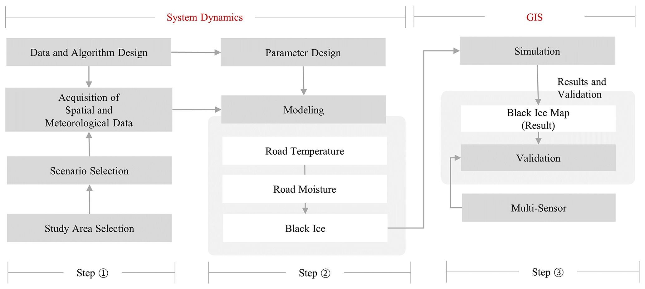
As shown in Fig. 1, the research was primarily composed of three stages. The first step was to establish the research methodology corresponding to Phase 2, which defined the study area, data, and algorithm. The second step, which corresponded to Phase 3, defined a scenario and derived modelling results. The road temperature and road moisture were calculated using system dynamics, and the amount and location of black ice were predicted. The third step, which corresponded to Phase 4, verified the model using a sensor. For the validation of the model, a hypothesis test (Z test, one-tailed test) was performed with a significance level of 0.05 for the section predicted by the model for the round force value, which was the core data. For the remaining data (water pressure, ultrasonic, temperature, and humidity), the model's validity was verified through fast Fourier transform, Z test, and graph comparison methods.
2.1 Model flow and data definition
This study attempted to model and simulate the occurrence of black ice, for which appropriate data selection was required. Before collecting the actual data, the data type and format were selected, and a system dynamics model that could handle the causal relationship between data (factors) was constructed. Powersim Studio version 10.0 was used as the software for operating the system dynamics method (Kim, 2021). A schematic of the system dynamics model designed in Powersim is shown in Fig. 2, which shows a causal map of the system dynamics structure. The causal map expresses the causal relationship of dynamic variables and directly describes the operating procedure of system dynamics (Kim, 2021; Forrester, 1994).
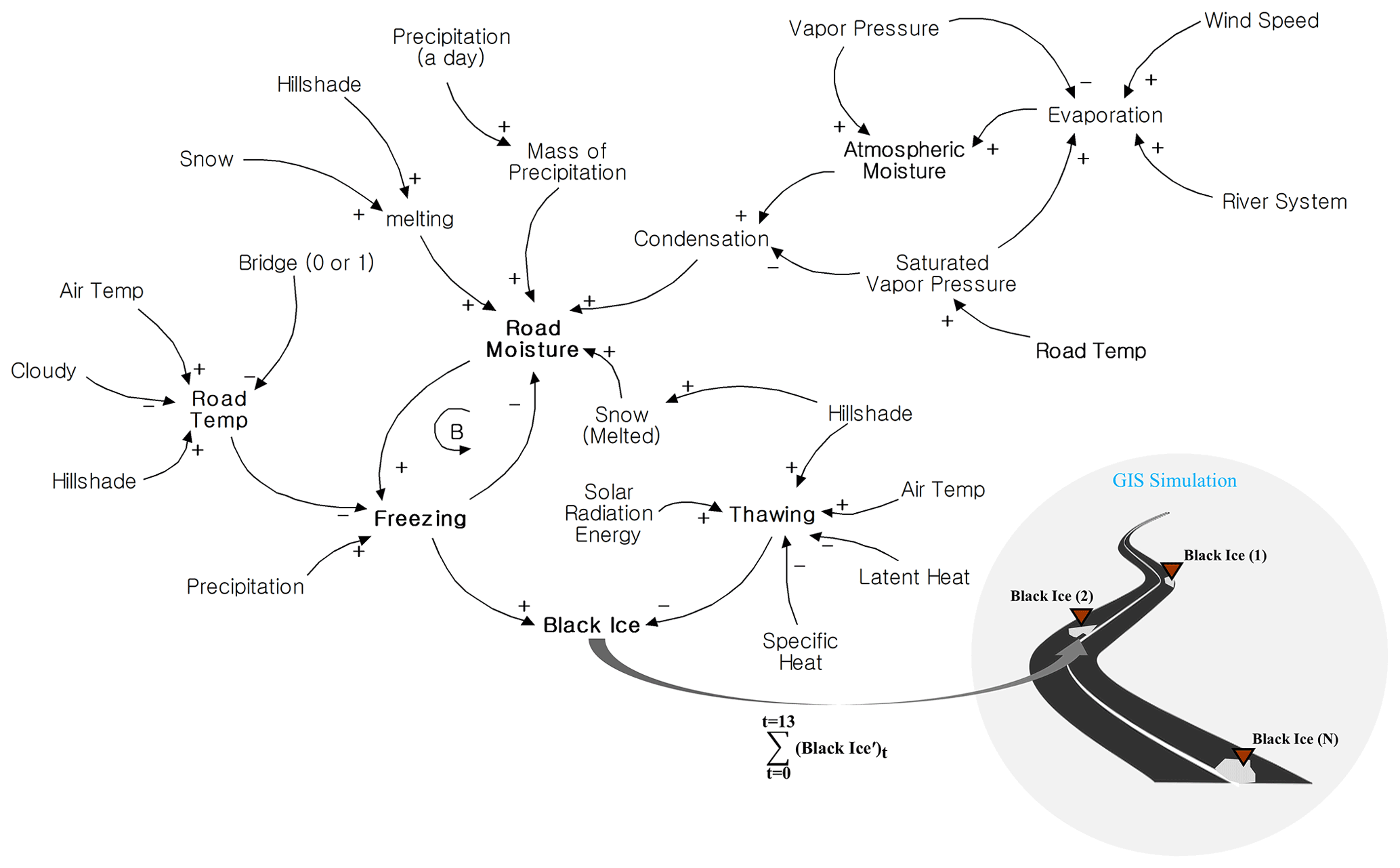
Figure 2Causal loop of system dynamics model. A causal loop is constructed according to the causal relationship of each factor, and the main results are road temperature, road moisture, and black ice. [+] means proportional, and [−] means inverse proportion.
The + and − signs in the causal map express causal relationships between the variables. In the case of +, the before and after factors are proportional and inversely proportional, respectively. In the causal map, B represents a balanced loop and maintains the total amount of a specific state. In the model used in this study, the relationship between road moisture and freezing corresponded to a balanced loop. In the final stage, freezing and black ice have a positive relationship, and thawing and black ice have a negative relationship (Sterman, 2000; Terzi et al., 2021). In other words, freezing and thawing per hour are determined by several factors, and the amount of black ice generated per hour is predicted accordingly. A system dynamics block diagram, which is the basis of the causal map in Fig. 2, is shown in Fig. A1.
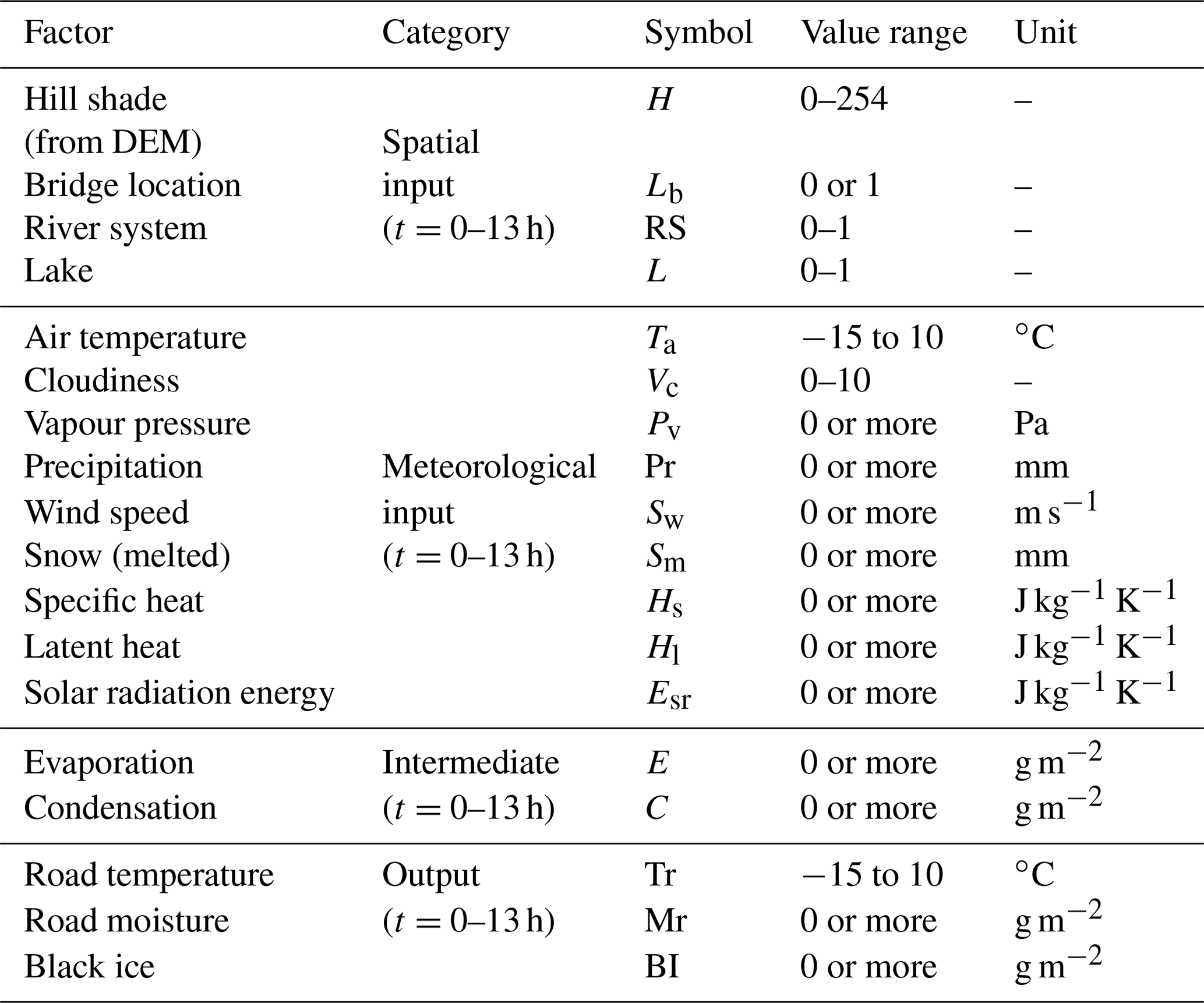
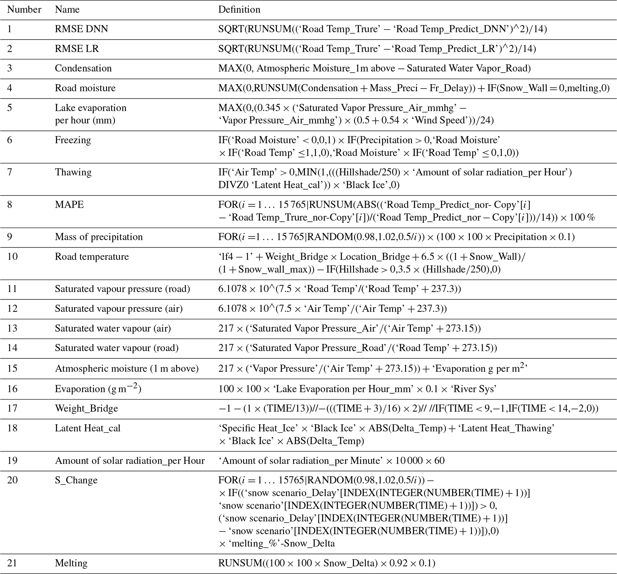
In the system dynamics model, spatial data are hill shade (from the digital elevation model, DEM), roads, bridges, river systems, and lakes, and weather data are air temperature, cloudiness, vapour pressure, precipitation, wind speed, snow (melted), specific heat, latent heat, and solar radiation energy. The system dynamics used in black ice modelling list the elements that cause specific phenomena on a block diagram and show their relationships over time. When spatial and meteorological data are entered into the system dynamics, they are calculated sequentially according to the causal relationship of the elements, and the output, black ice, is calculated through the intermediate factor. The intermediate factors, road temperature and road moisture, were calculated each time by reflecting the dynamic characteristics of the inputs. Road temperature is expressed as a function of hill shade, bridges, air temperature, and cloud cover, and road moisture is defined as a function of vapour pressure, precipitation, snow (melt), and wind speed. Black ice was predicted per hour according to the dynamic characteristics of the two intermediate factors. The expected amount and location of black ice generation were simulated using a GIS in units of square metres (Lysbakken and Norem, 2008; Nilssen, 2017; Schulson, 2013). Table 2 lists the required parameters. The model definition expressing the relational expressions between the significant factors is shown in Table A2.
2.2 Road temperature and moisture modelling
Road temperature and road moisture are important intermediate factors in the generation of black ice and were calculated as input data. These two factors are essential because freezing water on the road surface at sub-zero temperatures is the basic principle of black ice formation (Cary, 2010). The road temperature should be appropriately predicted to determine the formation of black ice. The existing prediction method required weather variables, such as solar radiation energy, air temperature, atmospheric pressure, wind, and thermal characteristic values, according to the road surface material (Park et al., 2014). However, this method requires many factors when predicting road temperature, and calculation errors can easily occur because of missing data. Given the nature of the simulation, which requires high efficiency and limited data, this area needs to be improved. In this study, we devised a method that can produce high prediction performance with a small number of input factors through the combination of a deep neural network (DNN) and an evolution algorithm (Peng et al., 2022).
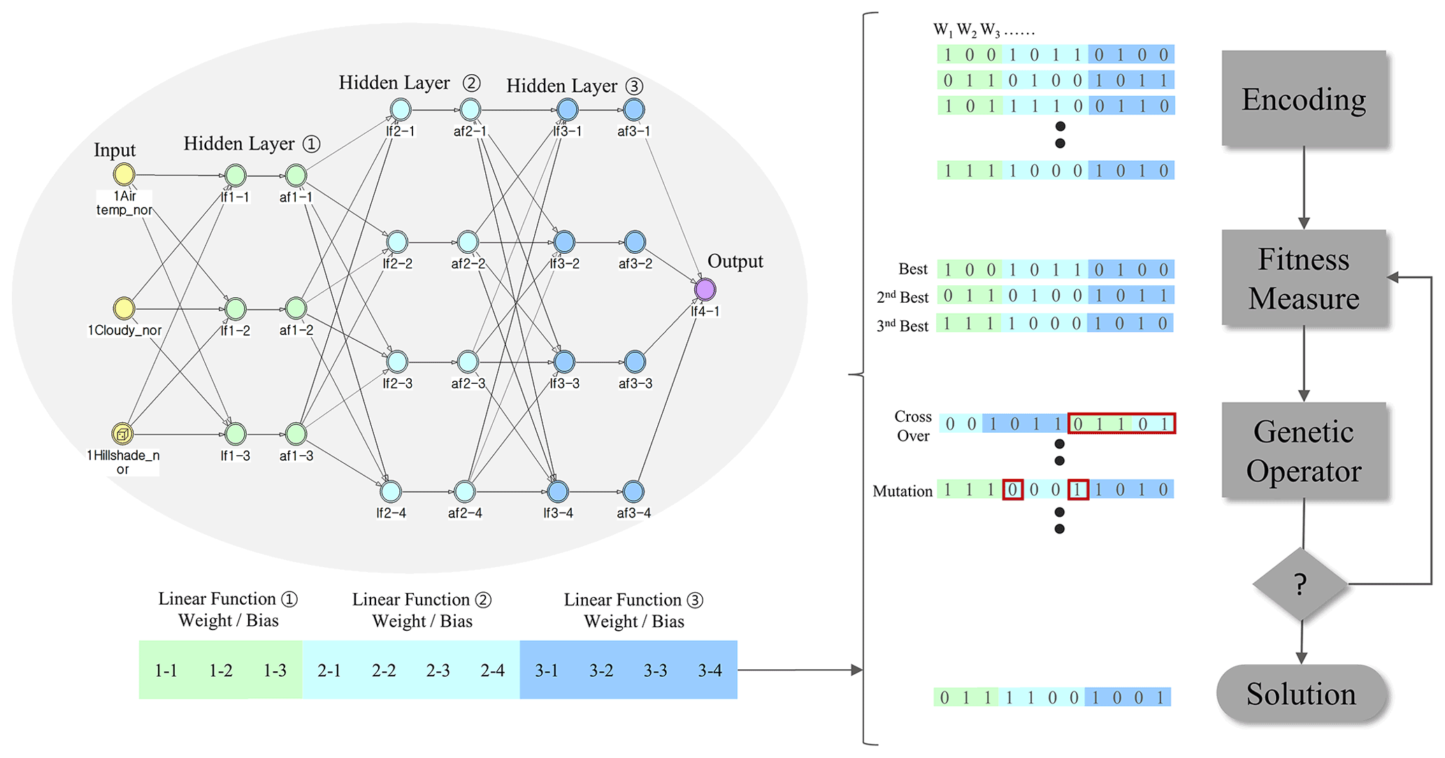
Figure 3Structure of system dynamics of deep neural network for road temperature modelling. (a) Change the parameters of DNN in the form of the chromosome. (b) The fitness function of the chromosome is evaluated and input to the genetic operator. (c) It performs selection to select chromosomes with high fitness, crossover to mix gene values, and mutations to simulate mutations in gene values. (d) Choose a solution based on the goodness of fit.
The factors entered into the deep neural network model were hill shade (H), air temperature (Ta), and cloudiness (C). Each factor is entered into the system dynamics by the following stock-flow model: variables (VRT, variable referring to road temperature) related to road temperature were entered using Eq. (1). The above-mentioned H, Lb, Ta, and C can be substituted for the variable VRT, which is calculated by adding the integral value according to time (t=0 to 13) to the initial value (t=0).
The road temperature can be directly predicted using the three variables of Eq. (1). Previous studies have used a linear regression model and evolution algorithm for road temperature prediction (Hong et al., 2021). The linear regression model parameters were trained using 98 datasets, including H, Lb, Ta, and C. However, when the number of data increases, the prediction ability becomes relatively low, and this method is not robust with various types of cases. In this study, 1498 datasets were obtained for H, Lb, Ta, and C, and a DNN model was introduced to predict road temperature in various weather conditions such as fog, rain, and snow. The structure of the DNN implemented in system dynamics is shown in Fig. 3. The DNN consists of three hidden layers: the first layer has three neurones, while the second and third layers have four neurones, and each neuron has weight and bias. Equation (2) is a linear function with a weight (wn) and bias (bn). Equation (3) is an activation function corresponding to the ReLU function. The ReLU function returns 0 when the input x value (lf) is less than 0 and returns the value as it is when the x value is greater than 0. As the maximum value can be greater than 1 when ReLU is used, vanishing gradients can be prevented, and the learning speed is faster (Kelleher, 2019).
The DNN block diagram of the system dynamics and schematic diagram of the evolution algorithm are shown in Fig. 3. Parameter (wn, bn) optimisation of the DNN model was performed using the evolution algorithm. The deep learning method based on the existing gradient descent and back propagation is quicker by dynamic programming but it is not suitable for application to the system dynamics environment with dynamic characteristics owing to the time change (Mitra et al., 2021). Therefore, the parameters of the DNN are optimised with the evolution algorithm, which is versatile for models with various characteristics such as dynamic change. Among the processes of the evolution algorithm, encoding involves changing the parameters of the model to be optimised into the genetic form of the evolution algorithm. If several candidates are generated by encoding, fitness is evaluated using a fitness function. The fitness function is given by Eq. (4). This is the mean absolute percentage error function between the actual and predicted values, and the termination condition is when it is minimum (De Myttenaere et al., 2016). When the parent solution is updated with solutions whose fitness is highly evaluated by the fitness function, the parent solutions are transferred to the genetic operator process to perform crossover and mutation. The child solutions created in the genetic operator process return to the fitness measure process, and the termination condition is evaluated. If the termination condition is not satisfied, the genetic operator is repeated, and the solution gradually converges. As the solution converged, the error between the predicted road temperature and the actual road temperature changed to the minimum value. A mean absolute percentage error (MAPE) value of 20 % or less implied appropriate prediction (reliability of 80 % or more) (Holland, 1984).
It is known that the temperature on bridges is 1–2 ∘C lower than that on general roads (Tabatabai and Aljuboori, 2017; Rathke and McPherson, 2006). Accordingly, we performed a temperature correction on the road passing through the bridge based on the road temperature prediction value. In Eq. (5), Tr is the road temperature, and time is the time in the simulation (∼0–13 h). Subsequently, reliability was used to evaluate the accuracy of the simulation train and test. Reliability is obtained by converting the F(t) value (MAPE) into a percentage and subtracting it from 100 %.
Road moisture must also be appropriately predicted to judge the formation of black ice. When moisture is formed on the road, it becomes possible to judge the generation of black ice over time with the dynamic characteristics of road temperature. There are three typical cases of moisture generation that cause black ice on roads (Zerr, 1997).
-
Case (1). Water vapour condenses on the road when the road temperature drops below the dew point.
-
Case (2). Freezing rainfalls occurs at below 0 ∘C road temperature.
-
Case (3). Water formation occurs when the accumulated snow melts due to the sun's heat.
Factors related to road moisture include vapour pressure, precipitation, wind speed, snow (melted), specific heat, latent heat, and solar radiation energy. The stock-flow model inputs vapour pressure, precipitation, wind speed, and snow (melted), such as road temperature factors, and their contents are the same as those in Eq. (8). The aforementioned Pv, Pr, Sw, and Sm can be substituted for the variable VRM (variable referring to road moisture), which is calculated by adding the integral value according to time (t=0–13) to the initial value (t=0).
The formula for road moisture (Mr) using condensation, mass of precipitation, and snow (melt) is as follows in Eq. (9). The mass of precipitation (MoP) is the mass of precipitation (g m−2), and C is the condensation (g m−2). If black ice occurs at freezing temperatures, road moisture is reduced. Fr means freezing per hour, as in Eq. (15).
Precipitation and mass of precipitation are weather-related factors on rainy days, as shown in Fig. 2. The MoP in Eq. (9) represents the actual mass of precipitation. In Eq. (10), P is the amount of precipitation (mm) converted to centimetres when the mass was calculated. MoP is measured in grams per square metre, and the length is 100 cm.
The condensation (C) in Eq. (9) is calculated using the equation between the amount of water vapour present in the atmosphere and the amount of saturated water vapour on the road. Condensation occurs when the temperature of water vapour in the atmosphere drops below the dew point on the road surface. The condensation contents are given by Eq. (11), where E is the evaporation (g m−2), V is the amount of vapour (g m−2), and Vs is the amount of saturated water vapour (g m−2).
The evaporation (E) in Eq. (11) is based on aerodynamics and Dalton's law describing evaporation. Dalton's law states that the movement of water molecules on a free surface is proportional to the vapour pressure gradient in the vertical direction. The formula for this theory is given by Eq. (12), where E is the amount of evaporation from the reservoir, es is the saturated water vapour pressure at air temperature (mm Hg), Pv is the actual vapour pressure at air temperature (mm Hg), and Sw is the wind speed (m s−1) at a height of 2 m from the water surface (Silberberg, 2009).
The amount of vapour (V) in Eq. (11) can be obtained using Eq. (13), where Pv is the vapour pressure, and Ta is the temperature of the air.
2.3 Black ice modelling and simulation
The amount and location of black ice generation per hour can be predicted by calculating the road temperature and road moisture. The black ice model is an integral value for the change in freezing (Fr) and thawing (Th) (Pradhan et al., 2019). Equation (14) is as follows:
Freezing is a function of the road temperature (Tr), road moisture (Mr), and precipitation (P). In the presence of road moisture, freezing changes when the road temperature reaches a specific condition. If the precipitation is greater than zero, freezing occurs when the road temperature is less than 1 ∘C (Imacho et al., 2002). If the precipitation is zero, freezing occurs when the temperature is below 0 ∘C (Bonanno et al., 2010). The contents are the same as those in Eq. (15).
Thawing is a function of black ice (BI), hill shade (H), air temperature (Ta), specific heat (Hs), latent heat (Hl), and solar radiation energy (Esr). The amount of energy required for thawing (Hn) was calculated as the sum of latent heat and specific heat (Pradhan et al., 2019). The air temperature is above or below zero and acts as a condition for thawing.
As shown in Fig. 2, the predicted amount and location of black ice per hour were simulated in units of square metres using the GIS. Black ice was modelled from 00:00 to 13:00 LT, the time range where the occurrence and traffic accidents were most frequent, and the total amount of black ice generated at all times was simulated in the GIS.
2.4 Black ice multi-sensor configuration and model validation
In this paper, sensor validation was performed on the model's point where black ice was predicted to occur. To determine the generation of black ice at the prediction point of the model, a black ice multi-sensor – that connects several sensors with the control board – was configured, as shown in Fig. 4.
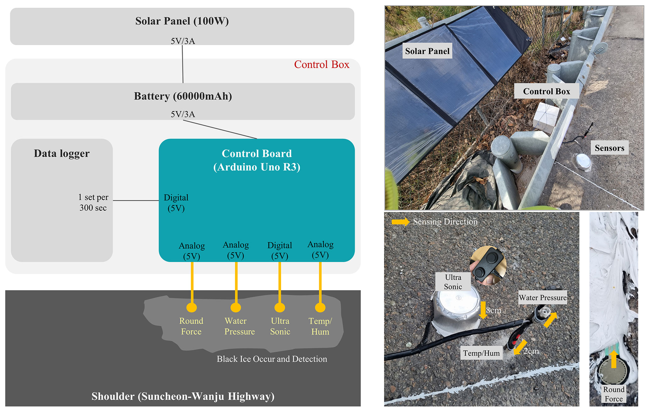
Figure 4Configuration and installation photo of multi-sensor for black ice detection. The sensing part of the round force and water pressure sensor faces upward, and the sensing part of the ultrasonic and temperature–humidity sensor faces downward.
The multi-sensor consisted of a round force (FSR402), water pressure (gravity: analogue water pressure sensor), ultrasonic (W238), and temperature/humidity (SHT30) sensor. The round force sensor was buried in the floor, and it detected the pressure of the black ice generated from the upper part. The water pressure sensor had a principle similar to that of the round force sensor, and it detected the pressure of moisture that entered the upper part and was frozen inside. In the case of the ultrasonic sensor, the area where the ultrasonic wave was emitted faced the floor; when black ice was generated, a height difference (default of 8 cm) was detected. Finally, the temperature/humidity sensor had a sensing part facing the ground, and the interval was ∼2 cm.
3.1 Black ice scenario
Gurye-gun, Jeollanam-do, Korea, was used as the study area, which is adjacent to the southern coast, and the water system and mountainous regions are evenly distributed inland. The highway in this area is prone to moisture and shade; as a result, it was expected to be prone to black ice (Shao and Lister, 1995). As shown in Fig. 5, the maximum elevation of Gurye-gun and Jeollanam-do is 1731 m (World Hillshade, 2020). The average elevation is 420.4 m, which corresponds to the representative mountainous region of Jeollanam-do. Jirisan, which belongs to Gurye-gun, is the highest mountain in Jeollanam-do, with a maximum elevation of 1916.77 m (Jirisan, 2022). The Suncheon–Wanju Highway in Gurye-gun, which is ∼16 km (Fig. 5a and b), passes through the water system and mountainous areas on the left and right (Fig. 5a and b), which is an environment prone to black ice. In addition, there are 10 bridges in the 16 km section. Bridges have an average temperature of 1–2 ∘C lower than that of general roads; therefore, black ice is more likely to occur even at the same temperature (Tabatabai and Aljuboori, 2017; Xue et al., 2018). Therefore, Gurye-gun in Jeollanam-do, an area vulnerable to black ice, was selected as the black ice research area, and data collection and modelling were performed.

Figure 5Suncheon–Wanju Highway, Gurye-gun, Jeollanam-do, a research area for system dynamics model. The Suncheon–Wanju Highway in Gurye-gun (16 km), Jeollanam-do, runs from point A (35∘18′ S) to point B (35∘10′ S). If the section from (a) to (b) is selected, and the cross-section is analysed, mountains and water systems are observed to the left and right (source: DEM created by the lidar method at the National Geographic Information Institute in Korea; https://www.ngii.go.kr/kor/content.do?sq=204, last access: 15 December 2021).
Actual days of black ice were selected as scenarios to verify the validity of the previously designed model. Data were acquired between 16–19 December 2021, by installing a multi-sensor that can detect black ice on a parted section of the Suncheon–Wanju Highway located in Gurye-gun, Jeollanam-do, South Korea. For this period, all three cases of fog (moisture), freezing rain, and snow (melted) could be confirmed; therefore, it was selected as a study scenario. The average values of the weather information for the relevant days are listed in Table 3. On 16 December, the maximum value of humidity was 100 %, and the temperature was a minimum of 0.3 ∘C; hence, it was analysed that fog had caused the freezing.
Table 3A list of scenarios for the system dynamics model. Validate the model by acquiring sensor data from the dates in the list.
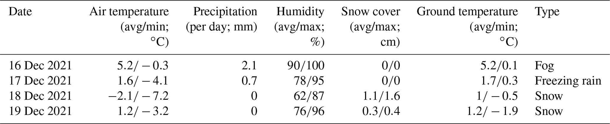
On 17 December, the temperature dropped below zero. The precipitation amount was 0.7 mm, and the lowest temperature was −4.1 ∘C, which was analysed to be freezing rain. It was interpreted that there was snow cover on 18–19 December, and there was a time when the air and ground temperature was 0 ∘C or higher. Hence, the snow melted, and the phenomenon of freezing occurred again (KMA, 2018). Therefore, 16 December was set as the fog scenario, 17 December as the freezing rain scenario, and 18 and 19 December as the snow scenario in this model.
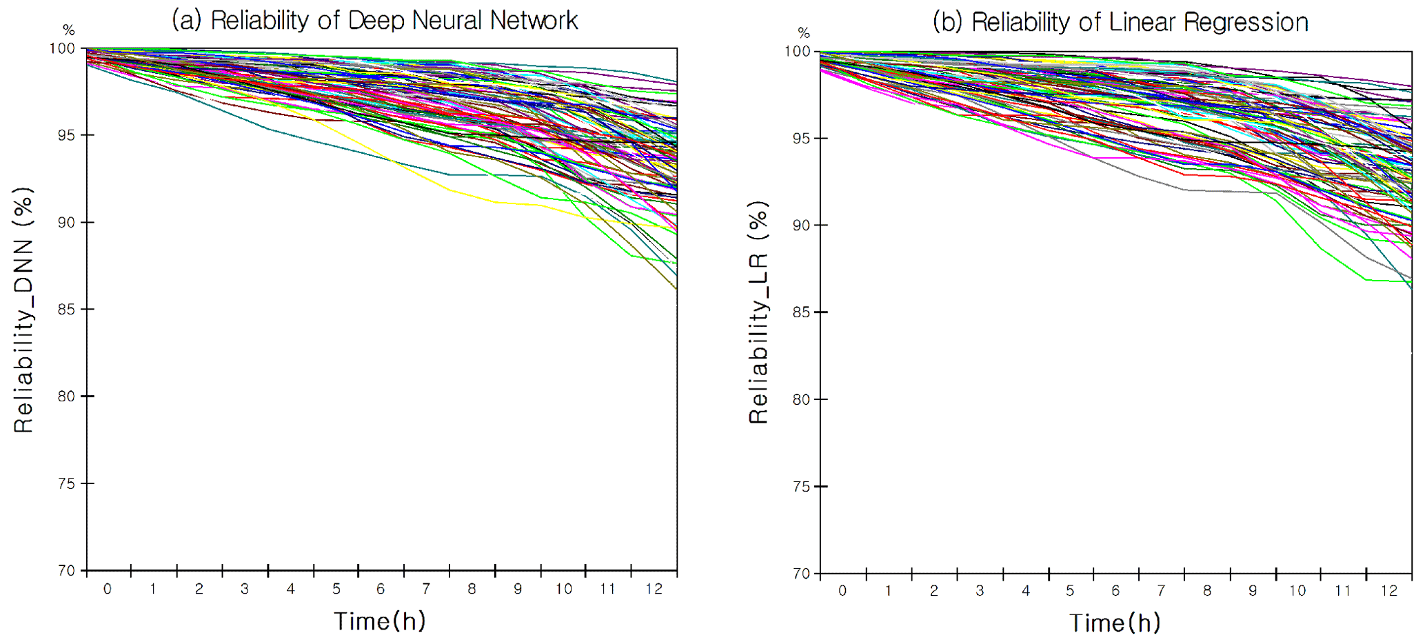
Figure 6Training reliability by combining system dynamics and machine learning when predicting road temperature. (a) The graph means the reliability of the deep neural network by data acquisition date, and the average value is 93.01 %. (b) The graph means the reliability of linear regression by data acquisition date, and the average value is 91.4 %. The parameters of the DNN model and the LR model were optimised with the evolution algorithm.
Table 4Factor list and data information of system dynamics model.
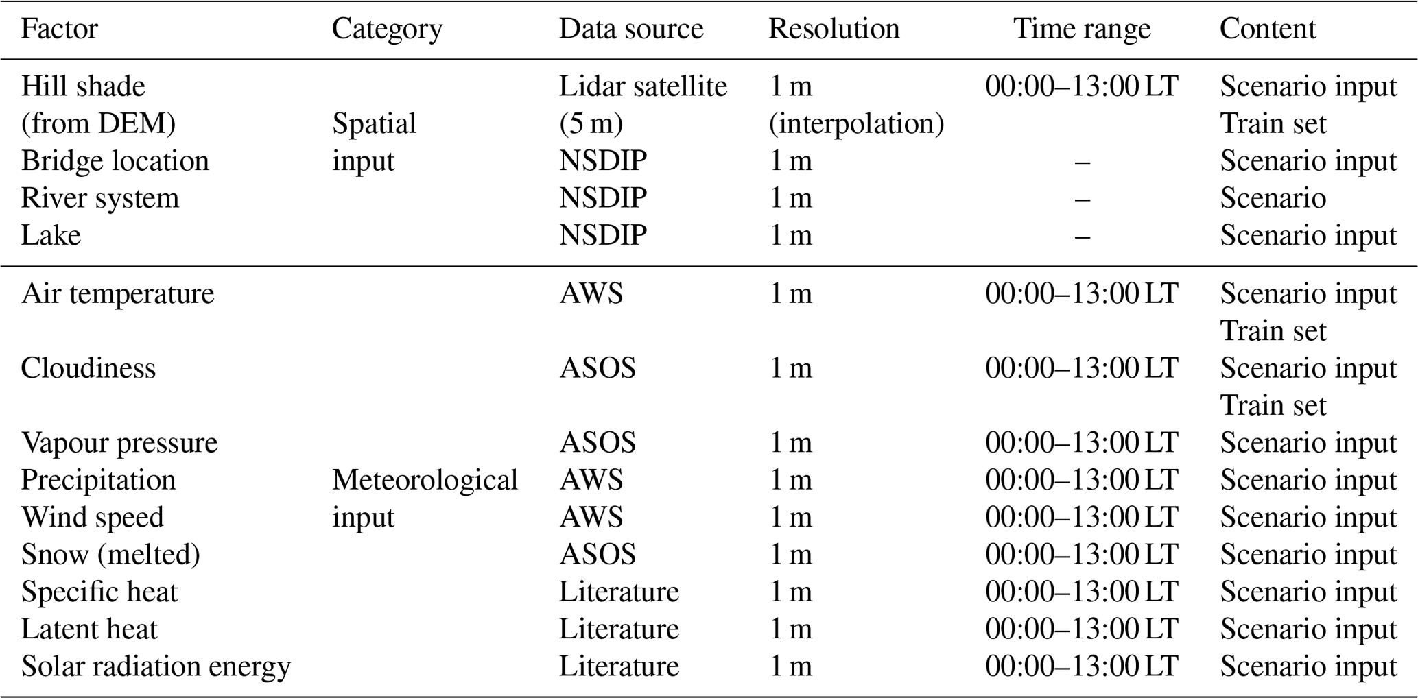
After establishing the scenario, the spatial and meteorological data for the selected date were entered into the model. Spatial data were obtained from the lidar satellite, National Spatial Data Infrastructure Portal (NSDIP), etc. Meteorological data were obtained from an automatic weather station (AWS) and an automated surface observing system (ASOS) operated by the Korea Meteorological Administration (KMA, 2018). The DEM had a resolution of 5 m and was interpolated to 1 m to produce the hill shade data. Bridges, roads, river systems, and lakes were converted into 1 m resolution raster information. The AWS, which acquired weather data, is located in Gurye and provides air temperature, wind speed, and precipitation data. However, with AWSs, the types of data that can be acquired are limited, so the remaining meteorological data were obtained from the ASOS in Suncheon, a nearby city. The data received from the ASOS were cloudiness, vapour pressure, and snow (melt). Specific heat, latent heat, and solar radiation energy were entered directly into the system dynamics without linking with the GIS. By obtaining the scientific experimental values through literature research, we can calculate the size of each point using the mass of ice and hill shade. The results are listed in Table 4. Hill shade and meteorological input data were from the period between 00:00 to 13:00 LT. As mentioned in Sect. 1, most black ice traffic accidents occurred from dawn to morning, and the average temperature reached its peak at 13:00 LT. For the efficiency of the simulation, the time range was set from early morning to 13:00 LT, when the amount of air temperature and solar radiation energy was low, but the traffic volume was high.
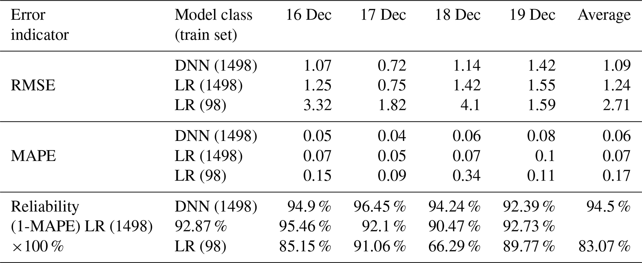
Table 5System dynamics and machine learning results for road temperature prediction. The results were expressed as RMSE, MAPE, and reliability of the model and actual data.
3.2 Black ice system dynamics modelling results
A DNN model was introduced to model road temperature, and an evolution algorithm was used for parameter optimisation. A total of 1498 training sets were used for parameter optimisation (weight and bias). Each set consisted of hill shade, air temperature, cloudy conditions, and road temperature. The training reliability obtained using the training set is shown in Fig. 6. Figure 6a and b show the training result reliability of the DNN and linear regression (LR), respectively. The reliability of the graph was recorded at time 13:00 LT. Previous studies used the LR model for road temperature prediction (Hong et al., 2021). The training reliability of the model of the previous study (RL) and that of the current study (DNN) were compared. The results were 93.01 % for DNN and 91.4 % for LR. In addition, when the root mean square error (RMSE) was applied as another error index, the DNN was 1.6, and LR was 1.67. That is, the training performance of the DNN was found to be better. After the training reliability was confirmed, it was derived by entering the test data into the DNN model. The DNN model performance test was conducted for ground temperature from 16–19 December 2021, the scenario date described above, from 00:00 to 13:00 LT. Based on the error indicators, the model test results are listed in Table 5.
Error and reliability values were derived according to the error indicator, model type, and scenario date. In the case of LR results, if the previous study method (Hong et al., 2021) could be introduced as it is, 98 datasets could be used. In the current study, 1498 datasets were used; therefore, there was a difference in the results. Hence, DNN (1498 datasets), LR (1498 datasets), and LR (previous studies, 98 datasets) were compared to analyse the superiority of the DNN model compared to linear regression. As a result, the average RMSE of the DNN model was improved by 13.8 % compared with the LR. In addition, the reliability (100 − MAPE × 100 %) of the DNN model was 1.77 % higher than that of the LR model. Compared to the previous study (LR, dataset: 97), the RMSE was improved by 148.6 %, and the reliability was increased by 11.43 %. Therefore, the DNN model had a higher prediction performance than the LR model; thus, the prediction value of the DNN model for road temperature was used.
The average road temperature for 16–19 December predicted by the DNN model is shown in Fig. 7. The lowest temperature on 16 December was predicted to be −0.31 ∘C, and the maximum temperature was 10.46 ∘C. The minimum temperature on 17 December was predicted to be 0.48 ∘C, and the maximum temperature was 4.74 ∘C. The lowest temperature on 18 December was predicted to be 0.17 ∘C, and the maximum temperature was 2.89 ∘C. The lowest temperature on 19 December was predicted to be −0.73 ∘C, and the maximum temperature was 3.36 ∘C. The predicted values of road temperature and road moisture were substituted into the model calculation process to predict the amount and location of the black ice.
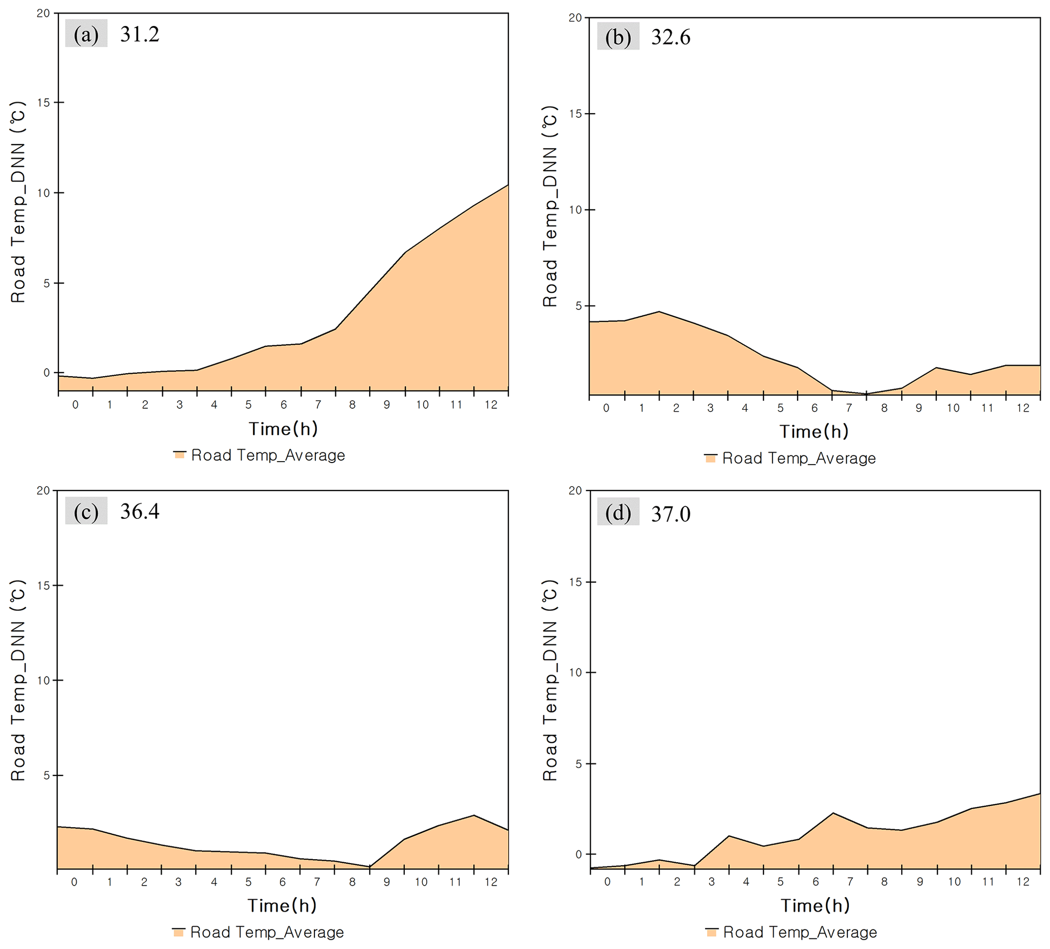
Figure 7Road temperature prediction results by system dynamics and DNN. (a) Prediction of road temperature for 16 December. (b) Prediction of road temperature for 17 December. (c) Prediction of road temperature for 18 December. (d) Prediction of road temperature for 19 December.
Road moisture was modelled based on the dynamic characteristics of the system dynamics, and black ice generation was modelled based on the predicted road temperature. The details of this process are shown in Fig. 8. All graphs in Fig. 8 show the average of 15 764 points on the Suncheon–Wanju Highway. Figure 8a–d show the amounts of precipitation, condensation, and road moisture. The maximum amount of road moisture on 16, 17, 18, and 19 December was predicted to be 2107.59, 540.12, 1502.61, and 487.21 g m−2, respectively. On 19 December, road moisture increased sharply as the accumulated snow melted. Figure 8e and f show the amount of black ice generated per hour due to “freezing” and “thawing”. The maximum amount of black ice on 16 December was predicted to be 0.72 g m−2; the black ice was formed before water accumulation due to precipitation. The maximum amount of black ice on 17 December was predicted to be 127.03 g m−2, as a result of freezing rain. The maximum amount of black ice on 18 and 19 December was predicted to be 14.36 and 17.91 g m−2, respectively, which was a result of road moisture formed by the melting of accumulated snow. The model results of specific points (points corresponding to 31.2, 32.6, 36.4, and 37.0 of the highway milestones) among 15 764 were compared with the sensor data.
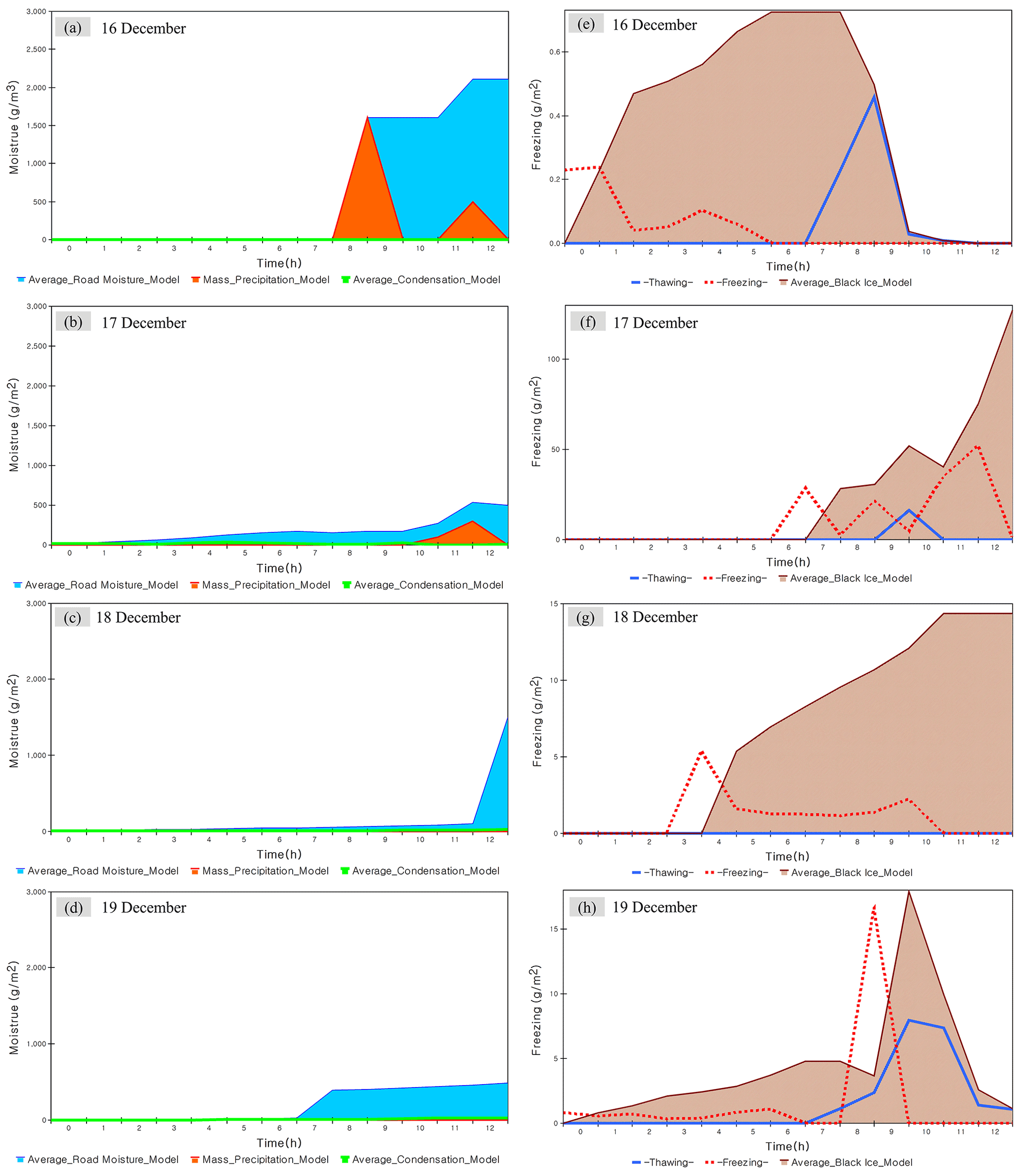
Figure 8Prediction of road moisture and black ice through system dynamics model. Panels (a–d) are the road moisture (calculated by condensation and precipitation) per hour on the road from 16–19 December. Panels (d–g) are black ice (calculated by freezing, thawing) per hour on the road from 16–19 December.
3.3 Black ice GIS simulation results
Figure 9 shows the simulation results of the amount and location of black ice predicted by the system dynamics modelling in the GIS (World_Imagery, 2020). The results of simulating the amount and location of black ice in units of square metres were exaggerated using the buffer function in the GIS. Figure 9a–d show the predicted location and generated amount of black ice between 16–19 December. The raster information of each black ice map was the average of the black ice generated from 00:00 to 13:00 LT on the selected day. The maximum amount of black ice formed during the 14 h period was (a) 31.5 g m−2, (b) 3715.79 g m−2, (c) 1861.93 g m−2, and (d) 697.86 g m−2, respectively, for each scenario date. The total amount of black ice generated, i.e. the average of all scenarios, was 1576.79 g m−2 (Fig. 9e). The days with the highest amount of black ice were 16 and 17 December, when freezing rain and snow occurred, respectively (Fig. 9b and c, respectively), and it was found that road moisture was higher, and road temperature was lower than on the other days.
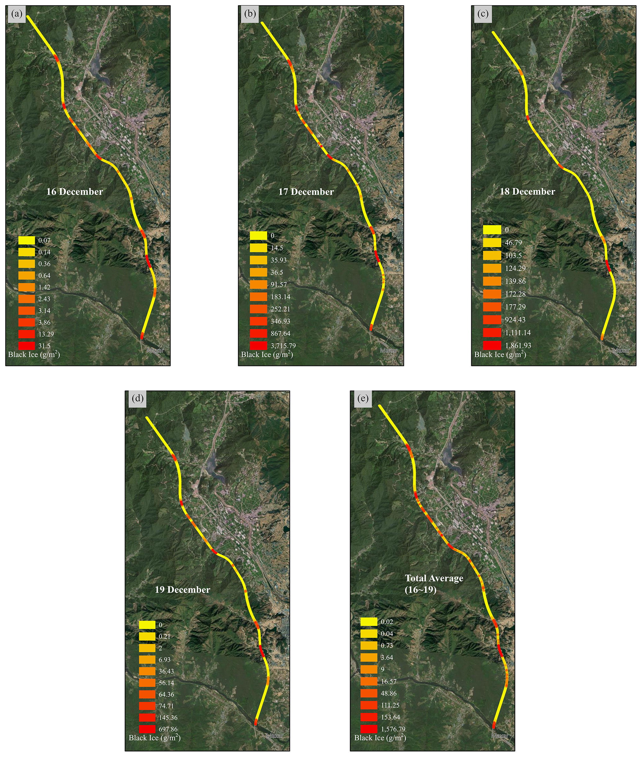
Figure 9Simulation of black ice occurrence prediction results of system dynamics in units of square metres in the GIS. Panels (a–d) show the amount and location of black ice from 16–19 December. (e) The average of the amount and location of black ice from 16–19 December (source: Esri, Maxar, Earthstar Geographics, and the GIS user community).
To discuss the modelling and simulation results, sensor data were acquired, and comparative validation was performed. Three points in the top two levels and one point in the bottom two levels were selected from the black ice map in Fig. 9e, which comprehensively covers all scenarios. Subsequently, the data were acquired from the sensor buried at the selected point. Multi-sensor data were collected from 16–19 December and statistically compared and analysed with the model to verify the system dynamics model.
After the black ice multi-sensor was positioned, data were acquired according to the scenario's date range (16–19 December). Points with signpost numbers 31.2, 32.6, 36.4, and 37.0 on the Suncheon–Wanju Highway were selected as burial points. Points 31.2, 32.6, and 37.0 corresponded to the top two levels of the amount of black ice prediction in Fig. 9e, and point 36.4 corresponded to the bottom two levels. The data acquired by date at the corresponding points included the round force, water pressure, ultrasonic force, temperature, and humidity. A graph of the multi-sensor burial point and the received data is shown in Fig. 10. For points 31.2, 32.6, and 37.0, data were acquired from 16–19 December. For the 36.4 points set as the comparison group by the result of model prediction, data of 16 December were acquired owing to the field situation. The round force sensor was analysed through an upper-tailed test with model prediction results (Raftery et al., 1995).
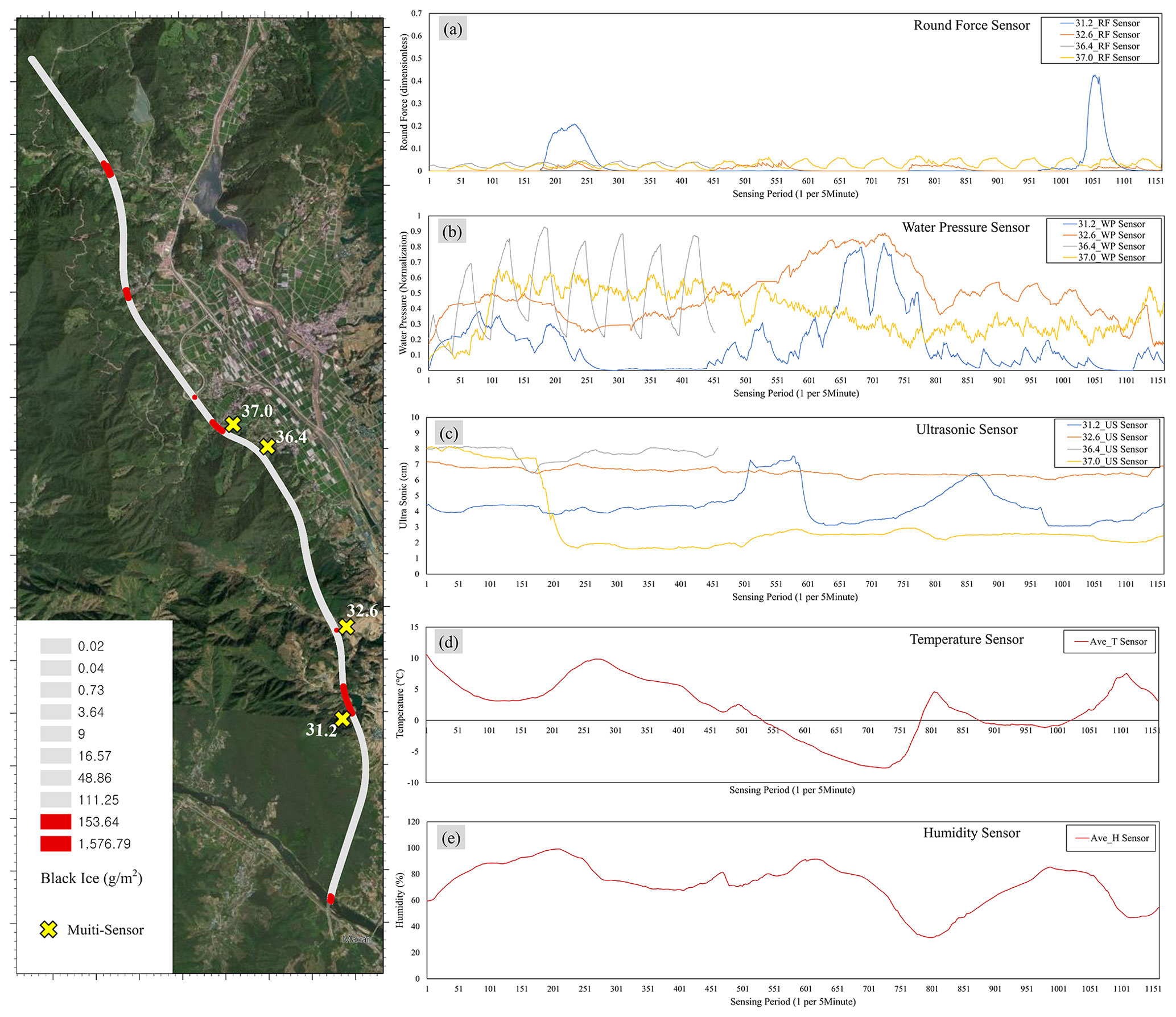
Figure 10The location of occurrence of black ice (top two levels) and data collection results for each sensor. Points 31.2, 32.6, and 37.0 are the experimental group, and point 36.4 is the comparison group. (a) Data graph of the round force sensor. (b) Data graph of the water pressure sensor. (c) Data graph of ultrasonic sensor. (d) Average temperature from temperature–humidity sensor. (e) Average humidity from temperature–humidity sensor (source: Esri, Maxar, Earthstar Geographics, and the GIS user community).
The water pressure sensor analysed the point where the frequency was constant using a fast Fourier transform to distinguish between the presence and absence of black ice (Rao et al., 2010). At point 36.4, where black ice was predicted to not occur, a signal with a constant frequency that is difficult to appear on ice was separated. The ultrasonic sensor was analysed through an upper-tailed test, such as a round force sensor. It was assumed that the data for 36.4, the point where black ice was predicted to not occur, would be significantly different when other sensor data were used as the population. The temperature–humidity sensor was compared and analysed to determine whether it was consistent with other sensors when the temperature dropped or humidity increased.
The white noise of the multi-sensor waveforms in Fig. 10 was corrected using a low-pass filter. In particular, the correction of white noise, which occurs mainly in analogue sensors, is essential for analysing data. The low-pass filter attenuates signals above the cutoff frequency and passes only signals below a specific frequency. The mathematical contents are as follows in Eq. (19), where “τ” is a time constant, and the larger the value, the greater the data correction, but a time delay occurs. The final correction value (yn) is calculated from the value corrected immediately before (yn−1) and the target value to be corrected (xn) (Kumngern et al., 2022; Roberts and Mullis, 1987).
4.1 Round force sensor analysis
The round force sensor provides the primary data that can determine the occurrence of black ice by time among the five sensors, and it was compared with the model by time unit. Figure 11 shows the buried position of the sensor and a graph comparing the sensor value and model. The graph in Fig. 11 shows a visualisation of the model (system dynamics) and RF (round force) sensor results in which the data collected by the RF sensor and the data predicted by the system dynamics overlap. It can be seen that the black ice occurrence range predicted by the model by point and time roughly coincided with the period when the sensor detected black ice. For the convenience of observation, sensor data arranged with a low-pass filter were included in the graph, but the analysis was performed including white noise before attenuation. The time period is approximately the same, but the difference in the trend in the graph's height is because of the model representing the amount of black ice (g m−2) and the sensor value being a force value (dimensionless). When the units and dimensions of the variables are different, a difference occurs in their maximum values. The data acquired at points 36.4 and 37.0 contain a certain noise pattern. It is interpreted that this is not an occurrence of black ice but an electrical error caused by the attachment of multiple sensors. An analysis was performed considering this phenomenon.
The Z test (upper-tailed test) was performed to analyse the graph in more detail on the RF sensor values detected in the time range that predicted black ice in the model. The P value derived from the Z-test result is the probability value that the research model indicates the null hypothesis to be correct but is wrong and is the probability that a specific alternative hypothesis will result in a type I error (error indicating that the null hypothesis is correct but is wrong). If the research hypothesis is tested with a 95 % confidence level, the significance level is set to 0.05 (α, 5 %). If the P value is less than 0.05, the null hypothesis is rejected, and the alternative hypothesis is adopted. The null and alternative hypotheses were established, and the P value was calculated to confirm whether the alternative hypothesis (research hypothesis) was acceptable (Raftery et al., 1995).
-
H0 (null hypothesis). The value of the round force sensor in the range predicted by the model is not different from other periods.
-
H1 (alternative hypothesis). The value of the round force sensor in the range predicted by the model is higher than that in other periods.
The formula used to obtain the standardised Z score of the performance value X of the sample data is as shown in Eq. (18), where X is the round force sensor value variable, μ is the population mean for the sensor value, σ is the population standard deviation, and n is the number of variables. The results of the upper-tailed test are shown in Table 6. The three points (31.2, 32.6, and 37.0) where black ice was predicted to occur had a P value lower than 0.05, so the null hypothesis was rejected, and the alternative hypothesis was adopted. It was interpreted that black ice occurred significantly at the corresponding point.

Figure 11Comparison graph of the data value of round force sensor and black ice prediction value of system dynamics model.
Table 6Z-test (upper-tailed test) result of round force sensor data value.
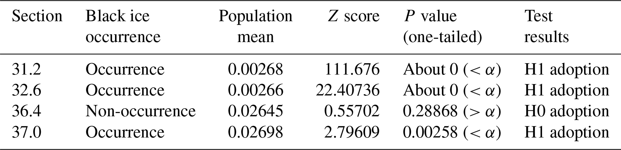
At point 37.0, where black ice was predicted to not occur, the P value was higher than 0.05; therefore, it was interpreted that black ice would not occur. Accordingly, it was confirmed that the round force sensor value and model result were the same, and the validity was verified.
4.2 Water pressure sensor analysis
Figure 10b shows a graph of water pressure, and voltage – which is a raw data value – was normalised to a value from 0 to 1 for ease of analysis. The graph of water pressure used a fast Fourier transform (FFT) to analyse the frequency trend and then determined whether black ice occurred by searching for a fixed frequency. FFT is an algorithm that rapidly calculates the discrete Fourier transform (DFT). DFT is as in Eq. (21). By decomposing a series of values into different frequencies, it is possible to check the waveforms of several trigonometric functions mixed in one signal. Although this operation is useful in many engineering fields, the direct calculation is not efficient; therefore, it is performed using FFT. The FFT quickly computes a transformation by factoring the DFT matrix into a product of sparse factors (Rao et al., 2010).
Figure 12 shows the result of the fast Fourier transform of the graph of the water pressure based on time. Figure 12a, b, and d show FFT graphs of points predicting that black ice will occur in the model, and Fig. 12c shows FFT graphs of points predicting that black ice will not occur in the model. The x axis represents the frequency of the FFT graph (S; Hz), and the y axis represents the amplitude. The FFT separates the periodic wavelengths in the signal in the frequency domain. It is assumed that if ice, not water, is frozen in the water pressure sensor, periodic wavelengths of relatively high frequencies can be observed. Therefore, at 0.00001 Hz (sample time: 300 s) in the graph of Fig. 12c, a sharp increase in amplitude was observed (0.27). A consistent waveform was observed at the indicated point in Fig. 12c, the control group, unlike the other points according to the amplitude value. It can be assumed that this is a property of the liquid that is not subjected to time-dependent stress owing to ice. At points 31.2, 32.6, and 37.0, where inconsistent wavelength was observed, irregular stress was generated due to ice, which was presumed to be compatible with the model results. At point 37.0, where a consistent wavelength was observed, no irregular stress was observed; therefore, it was presumed to be compatible with the model results.
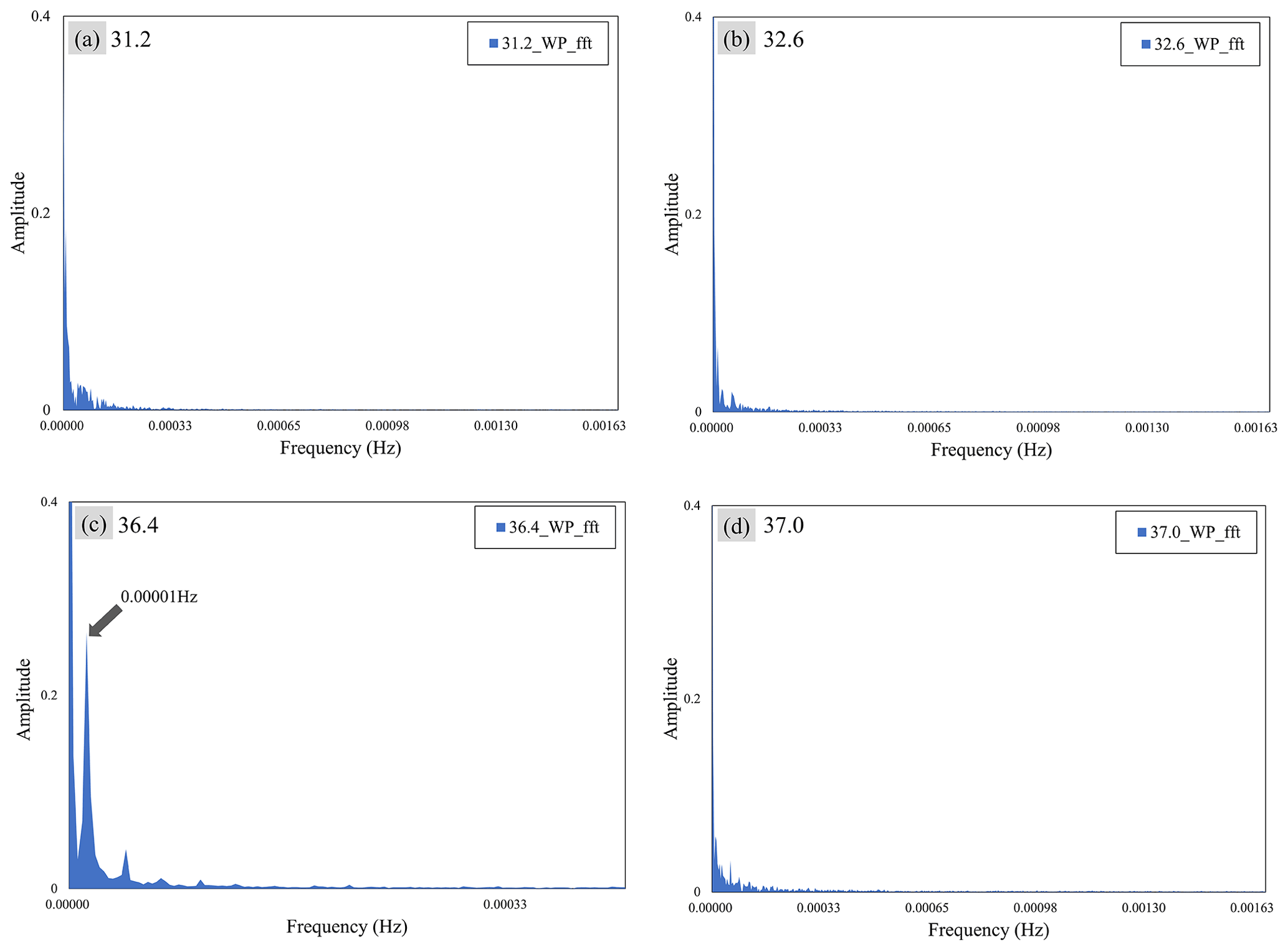
Figure 12Fast Fourier transform of the result of the data signal of the water pressure sensor. Panels (a), (b), and (d) indicate points where the system dynamics model predicted that black ice would occur, and no waveforms of a particular period were observed. Panel (c) indicates the point where the system dynamics model predicted that black ice did not occur, and a waveform of a particular period was observed.
4.3 Ultrasonic sensor analysis
Figure 10c shows an ultrasonic graph. The ultrasonic sensor data started with an initial value of 8 cm and decreased when the ice changed the height of the ground surface. It was hypothesised that the sensor value of 36.4, the point where black ice was predicted to not occur, would be significantly larger than the 31.2, 32.6, and 37.0 points predicted as the occurrence of black ice. The established hypothesis was tested using the Z test (upper-tailed test) for the alternative hypothesis (research hypothesis). The null and alternative hypotheses for point 36.4, the comparison group, are as follows.
-
H0 (null hypothesis). The ultrasonic value of the point predicted by the model as non-occurrence is not different from the point predicted by the occurrence.
-
H1 (alternative hypothesis). The ultrasonic value of the point predicted by the model as non-occurrence is different from that predicted as the occurrence.
As in the round force sensor analysis, if the P value is less than the significance level of 0.05, the null hypothesis is rejected, and the alternative hypothesis is adopted. The result of the upper-tailed test of the sample data at point 36.4 indicated a population mean of 4.67, standard deviation of 1.91, Z score of 34.17928, and P value of less than 0.00001. Since the P value was lower than the significance level (α=0.05), H0 (null hypothesis) was rejected, and H1 (alternative hypothesis) was adopted. According to the adoption of the alternative hypothesis, a research hypothesis is established: the ultrasonic value of the point predicted by the model as non-occurrence is different from the point predicted as the occurrence. Their contents are summarised in Table 7. Since the points 31.2, 32.6, and 36.4 are the population, and the point 36.4 is the sample, the hypothesis test was performed only on point 36.4 (Raftery et al., 1995).
Table 7Z-test (upper-tailed test) result of ultrasonic sensor data value.
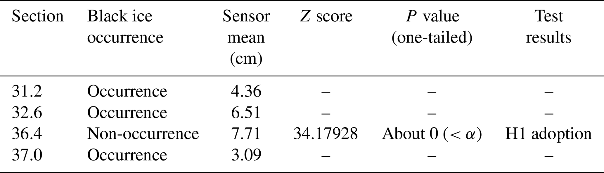
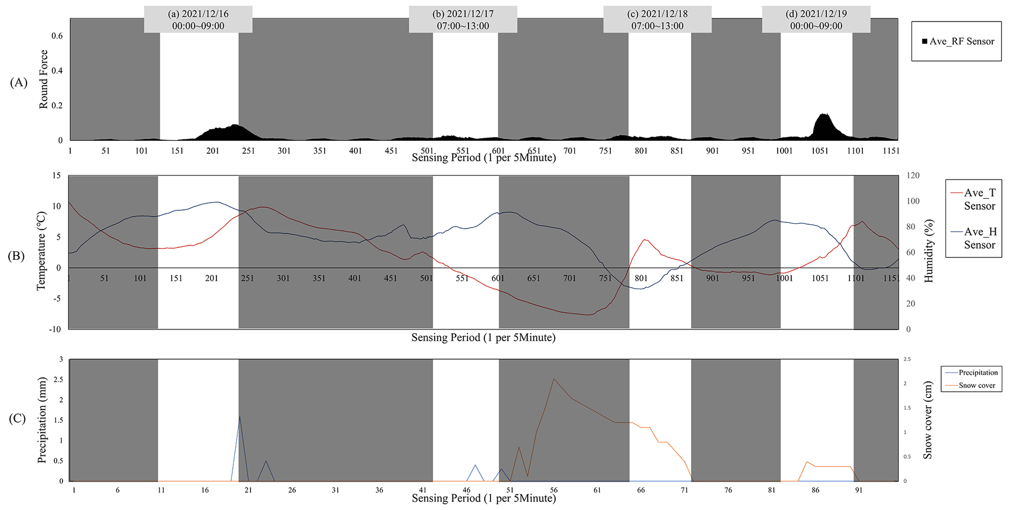
Figure 13Data analysis result of temperature/humidity sensor. Round force, temperature/humidity, precipitation, and snow cover were compared.
4.4 Temperature–humidity sensor and multi-sensor analysis
Figure 13 shows the average graph for the 31.2, 32.6, and 37.0 points where black ice significantly occurred among the round force, temperature, and humidity data. The highlighted bright areas (a–d) are time sections where black ice occurred in the system dynamics model. Figure 13 shows three graphs. (A) is a round force sensor, (B) is a temperature–humidity sensor, and (C) is precipitation (mm) and snow cover (cm) data obtained from the ASOS of the Korea Meteorological Administration for additional comparative analysis: (a) the average humidity exceeded 100 %, and the average temperature was a minimum of 2.98 ∘C. As previously analysed, this is an environment in which dew is formed by fog, and because all the points where black ice occurred significantly are near bridges, freezing occurred even at the temperature mentioned in the image. In the case of time, (b) it was found that black ice occurred because the temperature dropped to −3.28 ∘C at the lowest, with freezing rainfall, and (c) as shown in graph (C), snow cover was observed. As in (B), black ice occurred due to the low temperature of the road surface after the snow melted in the section where the temperature rose to a maximum of 6.25 ∘C. The snow cover exists in (d) as in (c), and (d) the snow that melted when the temperature rose to a maximum of 9.04 ∘C was frozen again at a low temperature. In conclusion, an environment prone to ice formation was observed when the model predicted that black ice would occur. In addition, in the round force graph in Fig. 13, the 31.2, 32.6, and 37.0 points were consistent with the model and the black ice occurrence trend. Temperature and humidity also created an environment that simultaneously formed black ice.
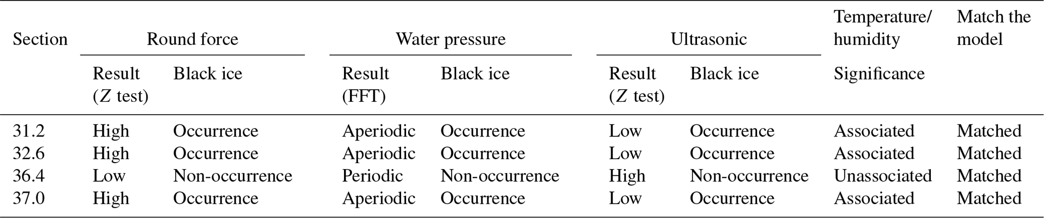
Table 8 shows the analysis results of the multi-sensor, a concept that includes both temperature/humidity and the sensors (round force, water pressure, ultrasonic) described above. Table 8 briefly shows the analysis results for the 31.2, 32.6, 36.4, and 37.0 points and sensors. At the 31.2, 32.6, and 37.0 points, where black ice occurrence was predicted by the model, the Z-test result of round force was “high”; the fast Fourier transform result of water pressure was “aperiodic”; the Z-test result of ultrasonic was “low”; and temperature/humidity was “associated”, implying “occurrence” of black ice. At the 36.4 point, where it was predicted that black ice does not occur, the Z-test result of round force was “low”; the fast Fourier transform result of water pressure was “periodic”; the ultrasonic Z-test result was “high”; and temperature/humidity was “unassociated”, implying “non-occurrence” of black ice.
This study modelled the amount and location of black ice using the system dynamics method and simulated it using the GIS. The amount of black ice generated per unit area (m2) was obtained as a block diagram constructed using the causal relationship between factors in the system dynamics model. The information input to the system dynamics model was meteorological and spatial data, and road temperature and moisture were calculated using these data. The road temperature was modelled using a DNN model and an evolution algorithm, and the road moisture was modelled numerically. Finally, the amount and location of black ice were predicted through numerical modelling combining road temperature and road moisture and simulated in units of square metres in the GIS. The study area was the Suncheon–Wanju Highway in Gurye-gun, Jeollanam-do, and modelling and simulations were performed from 16–19 December.
Based on the simulation results, multiple sensors were positioned at the 31.2, 32.6, 36.4, and 37.0 points on the Suncheon–Wanju Highway, and data were collected. The multi-sensor consisted of a round force, water pressure, ultrasonic force, and temperature–humidity sensor, and each sensor was analysed through a Z test and fast Fourier transform. For round force, using the Z test (upper-tailed test) through the P value, it was tested whether the predicted point where black ice would occur on the model matched the sensor value. Water pressure was used to analyse the surging value of the amplitude in the frequency domain using a fast Fourier transform to determine whether ice existed according to the periodic vibration. Ultrasonic Z tests were performed using the P value. It was verified that the height value of the comparison group (36.4 points) was significantly higher than that of the other points (31.2, 32.6, 37.0 points). Finally, the temperature and humidity were analysed at the point where black ice was predicted to occur in the model. In addition, the causal relationship between the round force analysed previously and precipitation and snow cover data obtained from the AWS of the Korea Meteorological Agency was comparatively analysed.
This study predicts the amount and location of black ice using system dynamics and the GIS. However, the prediction value of occurrence does not reflect other characteristics of traffic accidents related to society and the environment; therefore, it is not a complete concept to approach vulnerability. Hence, additional research on traffic accident vulnerability and risk is required. In addition, in the case of sensor technology, because the round force sensor is directly buried in the road shoulder, the actual occurrence trend of black ice can be checked over time; however, water pressure and ultrasonic sensors have different data collection environments (water pressure: collected inside the metal sensor; ultrasonic: cap to prevent snow accumulation). Therefore, it is possible to compare the experimental group (31.2, 32.6, and 37.0) and the comparison group (36.4) in the overall time, but the comparison at each time point is a matter to be further developed. Despite few shortcomings, the results of this study can provide useful data for government agencies (e.g. road traffic authorities) when managing traffic accidents caused by black ice. It should be noted that major factors have been added to the existing studies, the road temperature prediction rate has been improved by combining the DNN technique with system dynamics, and the system dynamics model has been verified using a multi-sensor. In the future, if various factors are supplemented for society and the environment, and a more accurate vulnerability and risk assessment is performed, it is possible to reduce the manpower wasted in the investigation by selecting the points where damage is expected from black ice in advance. It is also possible to apply structural or non-structural countermeasures at more precise points.

The data sources used for the case studies are listed in Table 4.
SBH and JK were involved in the conceptualisation. HSY and SKY developed the methodology. HSY supervised SBH and JK in the spatial and meteorological data processing. SBH explored the system dynamics modelling system and prepared input data. JK performed the connectivity analysis. SKY and SYR analysed the data. SBH and SYR developed the algorithm for data analysis and visualisation. ISJ wrote the manuscript draft and edited the co-authors' revisions. All co-authors were involved in the review of the manuscript.
The contact author has declared that none of the authors has any competing interests.
Publisher's note: Copernicus Publications remains neutral with regard to jurisdictional claims in published maps and institutional affiliations.
This research was supported by the National Research Foundation of Korea (NRF) grant funded by the Korean Government (MSIT) (no. 2021R1A2C201231911).
This paper was edited by Yves Bühler and reviewed by two anonymous referees.
Ali, S., Biermanns, P., Haider, R., and Reicherter, K.: Landslide susceptibility mapping by using a geographic information system (GIS) along the China–Pakistan Economic Corridor (Karakoram Highway), Pakistan, Nat. Hazards Earth Syst. Sci., 19, 999–1022, https://doi.org/10.5194/nhess-19-999-2019, 2019.
An, J. S. and Choi, S. W.: The role of winter weather in the population dynamics of spring moths in the southwest Korean peninsula, J. Asia-Pac. Entomol., 16, 49–53, https://doi.org/10.1016/j.aspen.2012.08.005, 2013.
Bardou, E. and Delaloye, R.: Effects of ground freezing and snow avalanche deposits on debris flows in alpine environments, Nat. Hazards Earth Syst. Sci., 4, 519–530, https://doi.org/10.5194/nhess-4-519-2004, 2004.
Bezrukova, N., Stulov, E., and Khalili, M.: A model for road icing forecast and control, in: Proc. SIRWEC (conference), 25–27 March 2006, Turin, Italy, 50–57, ID 234368645, 2006.
Bonanno, R., Loglisci, N., Cavalletto, S., and Cassardo, C.: Analysis of Different Freezing/Thawing Parameterizations using the UTOPIA Model, Water, 2, 468–483, 2010.
Cary, L.: Black ice, Vintage, New York, USA, ISBN 0-679-73745-6, 2010.
Chapman, L., Thornes, J. E., and Bradley, A. V.: Modelling of road surface temperature from a geographical parameter database. Part 2: Numerical, Meteorol. Appl., 8, 421–436, 2001.
Cheng, C. S., Auld, H., Li, G., Klaassen, J., and Li, Q.: Possible impacts of climate change on freezing rain in south-central Canada using downscaled future climate scenarios, Nat. Hazards Earth Syst. Sci., 7, 71–87, https://doi.org/10.5194/nhess-7-71-2007, 2007.
De Myttenaere, A., Golden, B., Le Grand, B., and Rossi, F.: Mean absolute percentage error for regression models, Neurocomputing, 192, 38–48, 2016.
Forrester, J. W.: System dynamics, systems thinking, and soft OR, Syst. Dynam. Rev., 10, 245–256, 1994.
Hayward, M. W., Whittaker, C. N., Lane, E. M., Power, W. L., Popinet, S., and White, J. D. L.: Multilayer modelling of waves generated by explosive subaqueous volcanism, Nat. Hazards Earth Syst. Sci., 22, 617–637, https://doi.org/10.5194/nhess-22-617-2022, 2022.
Holland, J. H.: Genetic algorithms and adaptation, in: Adaptive Control of Ill-Defined Systems, Springer, 317–333, https://doi.org/10.1007/978-1-4684-8941-5_21, 1984.
Hong, S.-B., Lee, B.-W., Kim, C.-H., and Yun, H.-S.: System Dynamics Modeling for Estimating the Locations of Road Icing Using GIS, Appl. Sci., 11, 8537, https://doi.org/10.3390/app11188537, 2021.
Hull, C.: Black Ice and Frozen Rain, Poetry-Rev., 89, 23–24, 1999.
Imacho, N., Nakamura, T., and Hashiba, K.: Road icing detection and forecasting system using optical fiber sensors for use in road management in winter, Hitachi Cable Rev., 21, 29–34, 2002.
Jeong, D. I., Cannon, A. J., and Zhang, X.: Projected changes to extreme freezing precipitation and design ice loads over North America based on a large ensemble of Canadian regional climate model simulations, Nat. Hazards Earth Syst. Sci., 19, 857-872, https://doi.org/10.5194/nhess-19-857-2019, 2019.
Jirisan: From Wikipedia, the free encyclopedia, https://en.wikipedia.org/wiki/Jirisan, last access: 27 April 2022.
Kämäräinen, M., Hyvärinen, O., Jylhä, K., Vajda, A., Neiglick, S., Nuottokari, J., and Gregow, H.: A method to estimate freezing rain climatology from ERA-Interim reanalysis over Europe, Nat. Hazards Earth Syst. Sci., 17, 243–259, https://doi.org/10.5194/nhess-17-243-2017, 2017.
Kangas, M., Heikinheimo, M., and Hippi, M.: RoadSurf: a modelling system for predicting road weather and road surface conditions, Meteorol. Appl., 22, 544–553, 2015.
Kelleher, J. D.: Deep learning, MIT Press, ISBN 9780262537551, 2019.
Kim, C. H.: System Dynamics, pybook, Seoul, Korea, ISBN 979-11-303-1239-2 93310, 2021.
KMA: Weather Data Service – Open MET Data Portal: ASOS (Automated Synoptic Observing System), https://data.kma.go.kr/cmmn/main.do (last access: 11 December 2020), 2018.
Koumoutsaris, S.: A hazard model of sub-freezing temperatures in the United Kingdom using vine copulas, Nat. Hazards Earth Syst. Sci., 19, 489–506, https://doi.org/10.5194/nhess-19-489-2019, 2019.
Kumngern, M., Khateb, F., and Kulej, T.: 0.5 V Current-Mode Low-Pass Filter Based on Voltage Second Generation Current Conveyor for Bio-Sensor Applications, IEEE Access, 10, 12201–12207, https://doi.org/10.1109/access.2022.3146328, 2022.
Lee, Y.-M., Oh, S.-Y., and Lee, S.-J.: A study on prediction of road freezing in Jeju, J. Environ. Science Int., 27, 531–541, 2018.
Liu, S. J., Nazarian, N., Hart, M. A., Niu, J. L., Xie, Y. X., and de Dear, R.: Dynamic thermal pleasure in outdoor environments – temporal alliesthesia, Sci. Total Environ., 771, 144910, https://doi.org/10.1016/j.scitotenv.2020.144910, 2021.
Liu, T., Pan, Q., Sanchez, J., Sun, S., Wang, N., and Yu, H.: Prototype Decision Support System for Black Ice Detection and Road Closure Control, IEEE Intel. Transport. Syst. Mag., 9, 91–102, https://doi.org/10.1109/mits.2017.2666587, 2017.
Lysbakken, K. and Norem, H.: The Amount of Salt on Road Surfaces after Salt Application, Surface Transportation Weather and Snow Removal and Ice Control Technology, Transportation research board of the national academies, 85–111, https://onlinepubs.trb.org/onlinepubs/circulars/ec126.pdf#page=97 (last access: 11 February 2022), 2008.
Mitra, R., Naruse, H., and Fujino, S.: Reconstruction of flow conditions from 2004 Indian Ocean tsunami deposits at the Phra Thong island using a deep neural network inverse model, Nat. Hazards Earth Syst. Sci., 21, 1667–1683, https://doi.org/10.5194/nhess-21-1667-2021, 2021.
Nilssen, K.: Ice melting capacity of deicing chemicals in cold temperatures, NTNU, ISBN 978-82-326-2581-9, 2017.
Park, M.-S., Joo, S. J., and Son, Y. T.: Development of road surface temperature prediction model using the Unified Model output (UM-Road), Atmosphere, 24, 471-479, 2014.
Peng, Y. Z., Gong, D. Q., Deng, C. Y., Li, H. Y., Cai, H. G., and Zhang, H.: An automatic hyperparameter optimization DNN model for precipitation prediction, Appl. Intell., 52, 2703–2719, https://doi.org/10.1007/s10489-021-02507-y, 2022.
Pradhan, N. R., Downer, C. W., and Marchenko, S.: Catchment Hydrological Modeling with Soil Thermal Dynamics during Seasonal Freeze-Thaw Cycles, Water, 11, 116, https://doi.org/10.3390/w11010116, 2019.
Raftery, A. E., Gilks, W., Richardson, S., and Spiegelhalter, D.: Hypothesis testing and model, Markov Chain Monte Carlo in Practice-Interdisciplinary statistics, Champman & Hall/CRC, 165–187, ISBN 978-0412055515, 1995.
Rao, K. R., Kim, D. N., and Hwang, J. J.: Fast Fourier transform: algorithms and applications, Springer, ISBN 978-1-4020-6629-0, 2010.
Rathke, J. M. and McPherson, R. A.: 4A.9 Modeling Road Pavement Temperatures With Skin Temperature Observations From The Oklahoma MESONET, in: 23rd International Conference on Interactive Information and Processing Systems for Meteorology, Oceanography and Hydrology, American Meteorological Society, https://www.researchgate.net/publication/237327551_Modeling_road_pavement_temperatures_with_skin_temperature_observations_from_the_Oklahoma_Mesonet (last access: 20 January 2022), 2006.
Roberts, R. A. and Mullis, C. T.: Digital signal processing, Addison-Wesley Longman Publishing Co., Inc., ISBN 0201163500, 1987.
Sass, B. H.: A Numerical Model for Prediction of Road Temperature and Ice, J. Appl. Meteorol., 31, 1499–1506, https://doi.org/10.1175/1520-0450(1992)031<1499:Anmfpo>2.0.Co;2, 1992.
Schulson, E.: Sliding heavy stones to the Forbidden City on ice, P. Natl. Acad. Sci. USA, 110, 19978–19979, 2013.
Shao, J. and Lister, P.: The prediction of road surface state and simulation of the shading effect, Bound.-Lay. Meteorol., 73, 411–419, 1995.
Silberberg, M. S. M. S.: Chemistry: the molecular nature of matter and change, McGraw-Hill, New York, USA, ISBN 0021442541, 2009.
Sterman, J.: Business Dynamics, McGrawHill, New York, USA, ISBN 007238915X, 2000.
Tabatabai, H. and Aljuboori, M.: A Novel Concrete-Based Sensor for Detection of Ice and Water on Roads and Bridges, Sensors, 17, 2912, https://doi.org/10.3390/s17122912, 2017.
Traffic Accident Analysis System: Traffic accident detailed statistics, http://taas.koroad.or.kr/web/shp/adi/initBasisPurps.do?menuId=WEB_KMP_IID_IID_PAB, last access: 1 January 2020.
Traffic accident article (case4): Chain collisions on Sangju-Yeongcheon Expressway due to black ice, http://www.joynews24.com/view/1231389 (last access: 26 December 2019), 2019a.
Traffic accident article (case5): What is black ice?, https://www.segye.com/newsView/20191129511652?OutUrl=naver (last access: 29 November 2019), 2019b.
Traffic accident article (case3): 41 car crash caused by black ice, http://news.tvchosun.com/site/data/html_dir/2020/01/06/2020010690068.html, last access: 6 January 2020.
Traffic accident article (case1): 170 fatalities in black ice traffic accidents in the last 5 years, https://www.yna.co.kr/view/AKR20210210121400530 (last access: 27 April 2022), 2022a.
Traffic accident article (case2): Ice accident on the way to work, https://www.mk.co.kr/news/society/view/2021/12/1113889/ (last access: 27 April 2022), 2022b.
Teke, M. and Duran, F.: The design and implementation of road condition warning system for drivers, Meas. Control, 52, 985–994, 2019.
Terzi, S., Sušnik, J., Schneiderbauer, S., Torresan, S., and Critto, A.: Stochastic system dynamics modelling for climate change water scarcity assessment of a reservoir in the Italian Alps, Nat. Hazards Earth Syst. Sci., 21, 3519–3537, https://doi.org/10.5194/nhess-21-3519-2021, 2021.
Toma-Danila, D., Armas, I., and Tiganescu, A.: Network-risk: an open GIS toolbox for estimating the implications of transportation network damage due to natural hazards, tested for Bucharest, Romania, Nat. Hazards Earth Syst. Sci., 20, 1421–1439, https://doi.org/10.5194/nhess-20-1421-2020, 2020.
Troiano, A., Pasero, E., and Mesin, L.: New system for detecting road ice formation, IEEE T. Instrum. Meas., 60, 1091–1101, 2010.
Wang, S., Mu, L., Yao, Z., Gao, J., Zhao, E., and Wang, L.: Assessing and zoning of typhoon storm surge risk with a geographic information system (GIS) technique: a case study of the coastal area of Huizhou, Nat. Hazards Earth Syst. Sci., 21, 439–462, https://doi.org/10.5194/nhess-21-439-2021, 2021.
World Hillshade: Elevation/World_Hillshade, https://services.arcgisonline.com/arcgis/rest/services/Elevation/World_Hillshade/MapServer, last access: January 2020.
World_Imagery: High Resolution Imagery, https://services.arcgisonline.com/ArcGIS/rest/services/World_Imagery/MapServer, last access: January 2020.
Xu, H., Zheng, J., Li, P., and Wang, Q.: Road icing forecasting and detecting system, AIP Conf. Proc., 1839, 020089, https://doi.org/10.1063/1.4982454, 2017.
Xue, J. Q., Lin, J. H., Briseghella, B., Tabatabai, H., and Chen, B. C.: Solar Radiation Parameters for Assessing Temperature Distributions on Bridge Cross-Sections, Appl. Sci.-Basel, 8, 627, https://doi.org/10.3390/app8040627, 2018.
Yi, Y., Zhang, Z., Zhang, W., Xu, Q., Deng, C., and Li, Q.: GIS-based earthquake-triggered-landslide susceptibility mapping with an integrated weighted index model in Jiuzhaigou region of Sichuan Province, China, Nat. Hazards Earth Syst. Sci., 19, 1973–1988, https://doi.org/10.5194/nhess-19-1973-2019, 2019.
Zerr, R. J.: Freezing rain: An observational and theoretical study, J. Appl. Meteorol., 36, 1647–1661, 1997.
- Abstract
- Introduction
- Methodology
- Results (application of black ice scenario)
- Discussion (black ice model sensor validation)
- Conclusion
- Appendix A: Block diagram structure and model definition of the system dynamics model
- Data availability
- Author contributions
- Competing interests
- Disclaimer
- Financial support
- Review statement
- References