Physically based modeling of co-seismic landslide, debris flow, and flood cascade

The 2008 Wenchuan earthquake lead to various complex multi-hazard chains that included seismically triggered landslide initiation, landslide runout, river damming, dam breaching, and flooding. The modeling of the interactions between such hazardous processes is challenging due to the complexity and uncertainty. Here we present an event-based physically based model that is able to simulate multi-hazard land surface process chains within a single unified simulation. The final model is used to simulate a multi-hazard chain event in the Hongchun watershed, where co-seismic landslides led to a landslide dam and, 2 years later, a debris flow that breached the landslide dam. While most aspects of the multi-hazard chain are predicted well, the correct prediction of slope failures remains the biggest challenge. Although the results should be treated carefully, the development of such a model provides a significant progress in the applicability of multi-hazard chain simulations.

1 Introduction

Many of the damaging events that involve land surface processes are not caused by individual but rather multiple interacting hazardous processes. Such combinations can take place because the same triggering events (e.g., extreme rainfall) trigger various hazardous processes (e.g., flash floods, landslides, and debris flows) that interact and that may impact the same elements at risk. For multi-hazard assessment, the hazard intensities and impact can differ significantly when compared to the individual hazardous processes (Gill and Malamud, 2014; Van Westen and Greiving, 2017). Hazardous events may also occur in sequence as cascading or domino events whereby one hazardous process triggers another either directly or later in time. One particular hazardous example of such cascading hazard events is the natural damming of rivers by landslides (Costa and Schuster, 1988; Walder and O'Conner, 1997). These landslide dams occur in mountainous landslide-prone areas around the world (Swanson et al., 1986; Chai et al., 2000; Dai et al., 2005; Korup, 2005; Harp and Crone, 2006; Nash et al., 2008; Liu et al., 2009; Fan et al., 2012). This sequence of hazardous events starts with a catastrophic slope failure, often caused by intense precipitation, a seismic trigger, or a combination of these. The released material moves downslope and can lose momentum through friction or by entering a sharply incised channel or river. When the volume of the solid materials is large enough, or when the moved landslide body retains mostly its original strength characteristics, it will form a barrier for water flow which will accumulate to form a dammed lake. Depending on the strength of the materials composing the dam, the barrier may breach when the barrier lake level exceeds the height of the dam due to either accelerated erosion, piping, or barrier collapse (Ermini and Casagli, 2003). During the breach, extreme discharges and solid-laden floods with high velocity may devastate the downstream areas (Schuster, 1993; Walder and O'Connor, 1997).

Natural dynamical systems such as the one described above can be complicated, containing many interactions and numerous fundamental processes related to hydrology and sediments (Walder and O'Conner, 1997). Slope failures, mass movement runout, and flooding are influenced by catchment-scale hydrology (Bout et al., 2018). Furthermore, inter-hazard interactions exist in many varieties, a review of which can be found in Kappes et al. (2012). In the case of landslide dam formation and breaching, many interactions exist between processes that are typically approached individually in modeling. Landslide dam-break floods have been analyzed using both empirical and physically based models (Evans, 1986; Costa and Schuster, 1988; Peng and Zhang, 2012). Empirical models are simpler to apply but provide less comprehensive results than physically based models. On the other hand, physically based models require detailed physical parameters as input and can be computationally costly. Whereas the individual components of the hazard chain – landslide initiation, landslide runout, dam breach, and flooding – have been modeled using physically based models, the interactions between these processes are generally not simulated within a single model due to their high complexity.

The prediction of landslide volumes resulting from earthquakes is a complex problem and requires specialized numerical models. Several physically based simulation tools for slope failure volume modeling have been developed, such as CLARA (Hungr et al., 1989), TSLOPE3 (Pyke, 1991), 3D-SLOPE (Lam and Fredlund, 1993), 3-DSLOPEGIS (Xie et al., 2003), r.slope.stability (Mergili et al., 2014a), Scoops3D (Reid et al., 2015), EDDA (Chen and Zhang, 2015), and OpenLISEM (Bout et al., 2018). CLARA, TSLOPE3, and 3D-SLOPE can only be applied on individual slopes, while r.slope.stability, Scoops3D, and OpenLISEM are spatially distributed models, which are based on geographic information systems (GISs). These can be applied for landslide volume estimation over a large area up to several hundred square kilometers. Numerical modeling of mass movement runout using two-dimensional approaches has been implemented in a variety of models (Malet et al., 2004; Rickenmann et al., 2006; Van Asch et al., 2007; Hürlimann et al., 2007; Domenech et al., 2019). They need detailed information on initial volume, rheology, and entrainment, as well as an accurate and detailed digital elevation model (DEM) (Hürlimann et al., 2007). Erosion, the water-driven uptake of sediment, and entrainment, the grain-driven uptake of sediment, have been used in understanding mass flow soil interactions. Erosion models, while traditionally focused on agricultural processes, come in great variety and provide insight into the flow–surface interactions. Examples are WEPP (Flanagan et al., 2001), EUROSEM (Morgan et al., 1998), and Delft3D Sediment (Roelvink and van Banning, 1995).

In the case of multi-hazard chains including landslide dams, integrated simulations face several critical issues. When a mass movement enters a channel with a certain water level, the landslide material mixes with the water in a dynamic manner, which is generally ignored in existing flow models such as Flo-2D (O'Brien et al., 1993). Similarly, the volumetric sediment content of water increases when a landslide dam is breached, and the material of the dam is entrained by the water flow. The entrainment of bed material is simulated in a limited number of spatial two-dimensional mass movement models but is rarely initiated from low-concentration water flow (Hungr et al., 2005). Several models have shown this functionality but lack the capability of modeling breaching behavior, and they ignore the resulting changes in the digital elevation model (Chen and Zhang, 2015; Hu et al.,2016; Baggio et al., 2021). Ignoring these changes makes the simulation of any breaching behavior impossible since increasing outflow must be the result of the entrainment of a flow path on the landslide dam.

Simplified coupled model approaches have been tested using separate and non-spatially distributed models for water flow and dam breaching. Empirical equations for dam-breach discharge have been developed and implemented by Singh and Snorasson (1984), Wang et al. (2008), and in the BREACH model (Fread, 1988). In these models, mathematical expressions for the dynamics of the outgoing discharge during a dam breach are derived from simplified landslide dam examples. Typically, a feedback loop between outflowing discharge and the amount of material entrained from the landslide dam determines the dynamics of the hydrograph. While these provide a useful estimation of the relevant physical processes during a dam breach, only outgoing discharge is simulated, and downstream processes are unknown. Moreover, the accuracy is generally low for more complicated cases (Zhu, 2006). The BREACH model simulates the increasing breach depth in a landslide dam using an iterative numerical solution. At the sides of the entrained channel, a limiting angle determines the additional collapse of material. Valiani et al. (2002) improved this by simulating dam-breach discharge using a two-dimensional finite element method.

Fan et al. (2012) provided an insightful step towards integrated modeling by linking a one-dimensional breach outflow model with a hydraulic two-dimensional flood simulation. The outflow from the BREACH model determines the boundary condition for the flood model (SOBEK). With this combined setup, it was possible to predict the dynamic dam breaching and the resulting large-scale flood behavior with significant accuracy. However, this integrated setup was still limited by the assumptions in the model. The breach model is one-dimensional and uses a simplified shape for the estimation of breaching dynamics. The setup ignores catchment-scale hydrological processes that could influence the surface flow. Furthermore, breach outflow can typically contain large amounts of solid material, altering the dynamics of the mixture. Fan et al. (2012) implemented a flood model in which flow is calculated using the Saint Venant equations for shallow flow, which ignores forces such as viscosity and implements a fluid-based frictional model (Dhondia and Stelling, 2002). Li et al. (2011a) provided a different approach to integrated simulations of landslide dams by linking the BREACH model with both a regional rainfall-runoff model and the Flo-2D debris flow model for modeling the runout of the breach material. Despite their improved method, the landslide dam-breach modeling depends on assumptions such as constant flow material properties, a limiting region for entrainment, and landslide initiation coming from pre-defined boundary conditions. More recently, Mergili et al. (2017) have shown the application of diluting mass flows to modeling glacial lake outburst floods. They developed the r.avaflow model, based on two-phase mixture equations by Pudasaini (2012), that allows for mixed flow of water and solids and implements a simplified entrainment process. However, this work does not take into account catchment-scale processes or actual landslide dam formation.

In this research, we aim to simulate a complex multi-hazard chain using a physically based integrated model. We aim to present an updated version of the OpenLISEM hazard model and analyze the application of this model to complex co-seismic hazard chains. The model includes a complete spatial simulation of a landslide dam process chain, including initial slope failure, landslide runout, deposition, lake formation, dam breaching, and flooding. To test the behavior of the developed model, simulations and validation will be shown for a case study of a dam-break flood event in the Hongchun watershed, which occurred in 2010 near the town of Yinxiu, close to the epicenter of the 2008 Wenchuan earthquake, in Sichuan Province, China. Finally, we investigate the predictive capabilities of complex multi-hazard multi-stage simulations by analyzing the sensitivity of the model to changes in input parameters.

The investigation of the Hongchun watershed builds on previous works in the literature. Tang et al. (2011, 2015) describe the co-seismic and post-seismic landslide events between 2008 and 2011 in this area. Several other studies have simulated the event using a variety of modeling techniques. Ouyang et al. (2015) applied shallow-flow depth-averaged debris flow equations in order to understand the event as a simplified runout process. Zhang et al. (2018) utilized a depth-averaged smooth particle hydrodynamics model to simulate both runout from landslides and the later debris flow. The authors show a novel application of such methods to a multi-stage event, however, without an integration in catchment-scale hydrology and a physical implementation of entrainment and breaching of the landslide dam. Domenech et al. (2019) used a multi-event debris flow model including entrainment to study the effect of material depletion on debris flow initiation in the Hongchun watershed. Using results of modeling studies, Chen et al. (2016) performed a cost–benefit analysis for the mitigation measures to protect the touristic town of Yinxiu, located directly opposite to the outlet of the Hongchun watershed on the other side of the Min River.

In this research, there is a focus on the integrated nature of the developed multi-hazard model. Multi-hazard multi-stage behavior is simulated for a series of interacting earthquake, landslide, debris flow, and flood processes in the Hongchun watershed. In order to simulate the behavior of this complex event, we develop an extended and improved version of OpenLISEM Hazard. To analyze the uncertainties in modeling such process chains, we employ ensemble simulations and analyze spatial hazard probabilities to estimate reliability. Finally, we discuss the benefits, downsides, and potential application of modeling methods that involve integrated multi-hazard process chains.

2 Theoretical model background

This section presents the theoretical background and governing equations for the components of our multi-hazard model. One of the important cornerstones is the work by Pudasaini (2012), who developed a set of physically based two-phase mass movement equations that can adapt the internal forces in the flow based on the local volumetric solid concentration. This allows us to simulate the behavior of landslides, the flow of water, and the interactions between mass movements and water flow (Mergili et al., 2018a). Using these equations, Bout et al. (2018) developed an integrated model for slope hydrology, slope failure, mass movements, and runout.

We have implemented a series of new processes within the physically based OpenLISEM Hazard model. In this section, we describe the relevant theory of existing functionality, as well as the addition of terrain-altering entrainment by mixture flows and the simulation of co-seismic shallow landslides. An overview of the processes is provided in Fig. 1.

Figure 1 A schematic overview of processes, fluxes, and storage within the OpenLISEM model.

2.1 Hydrology

The principle setup of the model starts with the surface aspects of the hydrological cycle. Spatially and temporally distributed rainfall forms the main input of water. We implement a set of equations for interception and micro-surface storage based on the original version of OpenLISEM (Jetten and de Roo, 2001; Baartman et al., 2012). The Green and Ampt infiltration model is implemented, which assumes a wetting front moving down into the soil due to infiltrating rainfall (Green and Ampt, 1911). The resulting potential infiltration is subtracted from the available surface water (Eq. 1).

$$\begin{array}{}\text{(1)}& f_{\mathrm{pot}}=-K_{\mathrm{s}}\left(\mathit{\psi }{\displaystyle \frac{{\mathit{\theta }}_s-{\mathit{\theta }}_i}{F}}+\mathrm{1}\right),\end{array}$$

where f_pot is the potential infiltration rate (m s⁻¹), F is the cumulative infiltrated water (m), θ_s is the porosity (m³ m⁻³), θ_i is the initial soil moisture content (m³ m⁻³), ψ is the matric pressure at the wetting front ($h=\mathit{\psi }+Z$) (m), and K_s is the saturated conductivity (m s⁻¹).

A separate modeling component is used to simulate several months of groundwater dynamics and generate the initial ground water conditions for the OpenLISEM Hazard simulation, which simulates the effects of a single rainstorm. Groundwater flow is estimated using a depth-averaged Darcy equation (Eq. 2), as is common in regional hydrological models (Van Beek, 2002).

$$\begin{array}{}\text{(2)}& V_{\mathrm{d}}=K_{\mathrm{s}}\cdot {\displaystyle \frac{\mathrm{d}h}{\mathrm{d}x}},\end{array}$$

where h is the hydraulic head (m), and V_d is the Darcy flow velocity (m s⁻¹).

2.2 Slope stability and failure

Hydrology influences slope stability and can eventually lead to failure. Slope failure is based on the iterative failure method (Bout et al., 2018). This technique reverses the factor of safety (Eq. 3) to solve for the remaining depth of material at which the local situation becomes stable. The locally altered terrain then results in changed forces in the surrounding cells. Through iteration, the method keeps removing material until no unstable cell is left and the minimum required material for a stable terrain has been removed. We added the seismic forcing in the factor of safety calculation following Morgenstern and Sangrey (1978).

$$\begin{array}{}\text{(3)}& \mathrm{FOS}={\displaystyle \frac{c^{\prime }+\left(\left(\left(\mathit{\gamma }-m{\mathit{\gamma }}_{\mathrm{w}}\right)h_{\mathrm{s}}+m{\mathit{\gamma }}_{\mathrm{w}}z\right)\cos {\left(\mathit{\beta }\right)}^{\mathrm{2}}-h_{\mathrm{s}}\mathit{\gamma }\mathit{\alpha }\sin \left(\mathit{\beta }\right)\cos \left(\mathit{\beta }\right)\right)\tan \left(\mathit{\varphi }\right)}{\left(\left(\mathit{\gamma }-m{\mathit{\gamma }}_{\mathrm{w}}\right)h_{\mathrm{s}}\right)\sin \left(\mathit{\beta }\right)\cos \left(\mathit{\beta }\right)+h_{\mathrm{s}}\mathit{\gamma }\mathit{\alpha }\cos {\left(\mathit{\beta }\right)}^{\mathrm{2}}}},\end{array}$$

where FOS is the factor of safety (−), β is the slope of the soil section (−), c^′ is the apparent cohesion of the soil (kPa), α is the peak horizontal earthquake acceleration (m s⁻²), ϕ is the internal friction angle of the soil (−), γ is the density of the slope material (kg m⁻³), γ_w is the density of water (kg m⁻³), m is the fraction of the soil depth that is saturated from the basal boundary (−), and h_s is the depth of the failure plane (m).

The apparent cohesion consists of additional root cohesion and a matric suction term. The acceleration is assumed to be, as in the most critical situation, the estimated peak horizontal ground acceleration. To account for subsurface force propagation, we include an iterative force solution. This is an extension of similar approaches in Cheng and Zhou (2013) and Chen et al., (2010). In the proposed implementation, forces are iteratively solved throughout the entire terrain description (Fig. 2).

Figure 2 Subsurface force distribution is solved through iteratively finding a steady state (Fd = driving force, Fc = resisting force).

In the three-dimensional case, where the x and y components of the seismic forcing and slope steepness influence the propagation, this can be expressed as Eq. (4).

$$\begin{array}{}\text{(4)}& \mathrm{\nabla }{\mathit{F}}_{\mathrm{up}}+\left(C-D\right)\cdot \left(\mathit{S}\cdot {\mathit{F}}_{\mathrm{lat}}\right)=\mathrm{0},\end{array}$$

with C the force capacity (numerator of Eq. 3), D the force demand (denominator of Eq. 3), S the normalized slope vector (−), and F_lat the vector of laterally acting forces (kg m s⁻²).

We assume that excess force is transferred downslope, but the fractured top material is unable to transfer force resistance upslope.

We assume in the setup of the model that a failure plane can develop in the soil materials at any depth. Equation (3) can be inverted to find the value of h, for which the safety factor is 1. To solve this equation for h, we first express the slope based on the local elevation differences and create a shortened equation for the factor of safety (Eqs. 5 and 6).

$$\begin{array}{}\text{(5)}& {\displaystyle }\mathit{\beta }=\mathrm{atan}\left({\displaystyle \frac{\max \left(z_{x-\mathrm{1}}-z_x,z_x-z_{x+\mathrm{1}}\right)}{\mathrm{d}x}}\right),\text{(6)}& {\displaystyle }\mathrm{FOS}=\mathrm{1}={\displaystyle \frac{C_{\mathrm{1}}+C_{\mathrm{2}}\cdot \cos {\left(\mathrm{atan}\left(\frac{z-z_{\mathrm{0}}}{\mathrm{d}x}\right)\right)}^{\mathrm{2}}\cdot \tan \left(\mathit{\varphi }\right)}{C_{\mathrm{3}}\cdot \sin \left(\mathrm{atan}\left(\frac{z-z_{\mathrm{0}}}{\mathrm{d}x}\right)\right)\cdot \cos \left(\mathrm{atan}\left(\frac{z-z_{\mathrm{0}}}{\mathrm{d}x}\right)\right)}},\end{array}$$

where the simplified constants are given by equations C₁=c, $C_{\mathrm{2}}=\left(\left(\mathit{\gamma }-m{\mathit{\gamma }}_{\mathrm{w}}\right)h_{\mathrm{s}}+m{\mathit{\gamma }}_{\mathrm{w}}{h}_{\mathrm{s}}\right)$, and $C_{\mathrm{3}}=\left(\left(\mathit{\gamma }-m{\mathit{\gamma }}_{\mathrm{w}}\right)h_{\mathrm{s}}\right)$, β is the slope angle (−), z is the elevation above the failure surface (m), and z₀ is the lowest neighboring elevation (m).

Solving this equation can be done using the trigonometric identities (Eqs. 7 and 8).

$$\begin{array}{}\text{(7)}& {\displaystyle }\cos \left(\mathrm{atan}\left(x\right)\right)={\displaystyle \frac{\mathrm{1}}{\sqrt{\mathrm{1}+x^{\mathrm{2}}}}}\text{(8)}& {\displaystyle }\sin \left(\mathrm{atan}\left(x\right)\right)={\displaystyle \frac{x}{\sqrt{\mathrm{1}+x^{\mathrm{2}}}}}\end{array}$$

Finally, we find the lowest real root to the second-order polynomial equation of the form

$$\begin{array}{}\text{(9)}& h_{\mathrm{s}}=a+\left(b\right)x+\left(c\right)x^{\mathrm{2}},\end{array}$$

where

$$\begin{array}{}\text{(10)}& {\displaystyle }a=C_{\mathrm{1}}{h}_{\mathrm{0}}^{\mathrm{2}}-{\mathrm{C}}_{\mathrm{1}}\mathrm{d}{x}^{\mathrm{2}},\text{(11)}& {\displaystyle }b=\mathrm{2}{C}_{\mathrm{1}}h\mathrm{0}-C_{\mathrm{3}}{h}_{\mathrm{0}}\mathrm{FOS}-C_{\mathrm{3}}{h}_{\mathrm{0}}\mathrm{FOS}\mathrm{d}x{C}_{\mathrm{2}}\mathrm{d}{x}^{\mathrm{2}},\text{(12)}& {\displaystyle }c=C_{\mathrm{1}}-C_{\mathrm{3}}\mathrm{FOS}\mathrm{d}x.\end{array}$$

Using Eq. (9) the critical depth can be found where the material on the slope is in equilibrium. By multiplying the area of a pixel with the slope material height above this critical depth, a failure volume can be calculated. This volume consists of solids and water, depending on the soil saturation level, and is then added to the flow equations that simulate Mohr–Coulomb mixture flow.

2.3 Flow dynamics

Once a volume of flowing material is introduced (either through hydrology or slope failure), its movement must be described. The dynamics of mass and momentum are calculated using a discretization of the continuity equation for mass and momentum of both solids and fluids (Eqs. 13, 14, and 15). Equation (13) described the conservation of mass, and Eq. (14) describes the conservation of momentum. On the left-hand side the storage term and advective terms are found. External forces and mass sources are added on the right-hand side.

$$\begin{array}{}\text{(13)}& {\displaystyle \frac{\partial h}{\partial t}}+{\displaystyle \frac{\partial \left(h{u}_x\right)}{\partial x}}+{\displaystyle \frac{\partial \left(h{u}_y\right)}{\partial y}}=R-I,\text{(14)}& {\displaystyle \frac{\partial h{u}_x}{\partial t}}+{\displaystyle \frac{\partial \left(h{u}_x^{\mathrm{2}}\right)}{\partial x}}+{\displaystyle \frac{\partial \left(h{u}_x{u}_y\right)}{\partial y}}=gh(S_x-S_{f,x}),\text{(15)}& {\displaystyle \frac{\partial h{u}_y}{\partial t}}+{\displaystyle \frac{\partial \left(h{u}_y^{\mathrm{2}}\right)}{\partial y}}+{\displaystyle \frac{\partial \left(h{u}_x{u}_y\right)\partial x}{=}}gh(S_y-S_{f,y}),\end{array}$$

with h being the flow height (m), u the flow velocity (m s⁻¹), R the rainfall (m), I the infiltration (m), g the gravitational acceleration (m s⁻²), S the friction term (m s⁻²), and S_f the momentum source term (m s⁻²).

The momentum source terms predominantly determine the behavior of the flow. Here we implement pressure and friction forces for fluids as is typical for shallow water assumptions (O'Brien et al., 1993).

$$\begin{array}{}\text{(16)}& {\displaystyle }{S}_x=-{\displaystyle \frac{d\left(\frac{g{h}^{\mathrm{2}}}{\mathrm{2}}\right)}{\mathrm{d}x}}-gh{S}_{f_x},\text{(17)}& {\displaystyle }{S}_y=-{\displaystyle \frac{d\left(\frac{g{h}^{\mathrm{2}}}{\mathrm{2}}\right)}{\mathrm{d}y}}-gh{S}_{f_y}.\end{array}$$

The friction slope terms, which are the friction forces divided by the water height and the gravitational acceleration, can be calculated using the Darcy–Weisbach friction law (Chow, 1959) (Eq. 16).

$$\begin{array}{}\text{(18)}& S_{\mathrm{f}}={\displaystyle \frac{g}{n^{\mathrm{2}}}}{\displaystyle \frac{\mathit{u}\left|\mathit{u}\right|}{h^{\frac{\mathrm{4}}{\mathrm{3}}}}},\end{array}$$

with n being the Manning's n friction coefficient (s m^−⅓).

The momentum source terms within OpenLISEM Hazard are based on the work by Pudasaini (2012). This set of equations contains a physically based two-phase momentum balance. Besides pressure and gravitational forces, it includes viscous forces, non-Newtonian viscosity, two-phase drag, and a Mohr–Coulomb type friction force for the solid phase (Eqs. 19, 20, 21, 22). Based on the current and local state of flow, forces change in magnitude. This approach allows for a smooth transition between non-viscous flow, hyper-concentrated streamflow, debris flows, or landslide runout by automatically scaling and solving the interactions between solids and fluids.

$$\begin{array}{}\text{(19)}& {\displaystyle }\begin{array}{rl}{S}_{x,s}& ={\mathit{\alpha }}_{\mathrm{s}}\left(g\left({\displaystyle \frac{\partial b}{\partial x}}\right)-{\displaystyle \frac{u_s}{\left|{\mathit{u}}_s\right|}}\tan \left(\partial P_{b_s}\right)-\mathit{\epsilon }{P}_{{\mathrm{b}}_{\mathrm{s}}}\left({\displaystyle \frac{\partial b}{\partial x}}\right)\right)\\ & -\mathit{\epsilon }{\mathit{\alpha }}_s\mathit{\gamma }{P}_{{\mathrm{b}}_{\mathrm{f}}}\left({\displaystyle \frac{\partial h}{\partial x}}+{\displaystyle \frac{\partial b}{\partial x}}\right)\\ & +C_{\mathrm{DG}}\left(u_f-u_s\right){\left|{\mathit{u}}_f-{\mathit{u}}_s\right|}^{j-\mathrm{1}}\end{array}\text{(20)}& {\displaystyle }\begin{array}{rl}{S}_{y,s}& ={\mathit{\alpha }}_{\mathrm{s}}\left(g\left({\displaystyle \frac{\partial b}{\partial y}}\right)-{\displaystyle \frac{v_s}{\left|{\mathit{u}}_s\right|}}\tan \left(\partial P_{b_s}\right)-\mathit{\epsilon }{P}_{{\mathrm{b}}_{\mathrm{s}}}\left({\displaystyle \frac{\partial b}{\partial y}}\right)\right)\\ & -\mathit{\epsilon }{\mathit{\alpha }}_s\mathit{\gamma }{P}_{{\mathrm{b}}_{\mathrm{f}}}\left({\displaystyle \frac{\partial h}{\partial y}}+{\displaystyle \frac{\partial b}{\partial y}}\right)\\ & +C_{\mathrm{DG}}\left(v_f-v_s\right){\left|{\mathit{u}}_f-{\mathit{u}}_s\right|}^{j-\mathrm{1}}\end{array}\text{(21)}& {\displaystyle }\begin{array}{rl}{S}_{x,f}& ={\mathit{\alpha }}_{\mathrm{f}}\left\{g\left({\displaystyle \frac{\partial b}{\partial x}}\right)-\mathit{\epsilon }\left[{\displaystyle \frac{\mathrm{1}}{h}}{\displaystyle \frac{\partial }{\partial x}}\left({\displaystyle \frac{h^{\mathrm{2}}}{\mathrm{2}}}{P}_{b_f}\right)+P_{b_f}{\displaystyle \frac{\partial b}{\partial x}}\right.\right.\\ & -{\displaystyle \frac{\mathrm{1}}{{\mathit{\alpha }}_{\mathrm{f}}{N}_{Re}}}\left(\mathrm{2}{\displaystyle \frac{{\partial }^{\mathrm{2}}{u}_f}{\partial x^{\mathrm{2}}}}+{\displaystyle \frac{{\partial }^{\mathrm{2}}{v}_f}{\partial y\partial x}}+{\displaystyle \frac{{\partial }^{\mathrm{2}}{u}_f}{\partial y^{\mathrm{2}}}}-{\displaystyle \frac{\mathit{\chi }{u}_f}{{\mathit{\epsilon }}^{\mathrm{2}}{h}^{\mathrm{2}}}}\right)\\ & +{\displaystyle \frac{\mathrm{1}}{{\mathit{\alpha }}_{\mathrm{f}}{N}_{Re}}}\left(\mathrm{2}{\displaystyle \frac{\partial }{\partial x}}\left({\displaystyle \frac{\partial {\mathit{\alpha }}_{\mathrm{s}}}{\partial x}}\left(u_f-u_s\right)\right)\right.\\ & \left.+{\displaystyle \frac{\partial }{\partial y}}\left({\displaystyle \frac{\partial {\mathit{\alpha }}_s}{\partial x}}\left(v_f-v_s\right)+{\displaystyle \frac{\partial {\mathit{\alpha }}_s}{\partial y}}\left(u_f-u_s\right)\right)\right)\\ & \left.\left.-{\displaystyle \frac{\mathit{\xi }{\mathit{\alpha }}_s\left(v_f-v_s\right)}{{\mathit{\epsilon }}^{\mathrm{2}}{\mathit{\alpha }}_{\mathrm{f}}{N}_{R{e}_A}{h}^{\mathrm{2}}}}\right]\right\}-{\displaystyle \frac{\mathrm{1}}{\mathit{\gamma }}}{C}_{\mathrm{DG}}\left(u_f-u_s\right)\\ & {\left|{\mathit{u}}_f-{\mathit{u}}_s\right|}^{j-\mathrm{1}}\end{array}\text{(22)}& {\displaystyle }\begin{array}{rl}{S}_{y,f}& ={\mathit{\alpha }}_{\mathrm{f}}\left\{g\left({\displaystyle \frac{\partial b}{\partial y}}\right)-\mathit{\epsilon }\left[{\displaystyle \frac{\mathrm{1}}{h}}{\displaystyle \frac{\partial }{\partial y}}\left({\displaystyle \frac{h^{\mathrm{2}}}{\mathrm{2}}}{P}_{b_f}\right)+P_{b_f}{\displaystyle \frac{\partial b}{\partial y}}\right.\right.\\ & -{\displaystyle \frac{\mathrm{1}}{{\mathit{\alpha }}_{\mathrm{f}}{N}_{Re}}}\left(\mathrm{2}{\displaystyle \frac{{\partial }^{\mathrm{2}}{v}_f}{\partial y^{\mathrm{2}}}}+{\displaystyle \frac{{\partial }^{\mathrm{2}}{u}_f}{\partial y\partial x}}+{\displaystyle \frac{{\partial }^{\mathrm{2}}{v}_f}{\partial y^{\mathrm{2}}}}-{\displaystyle \frac{\mathit{\chi }{v}_f}{{\mathit{\epsilon }}^{\mathrm{2}}{h}^{\mathrm{2}}}}\right)\\ & +{\displaystyle \frac{\mathrm{1}}{{\mathit{\alpha }}_{\mathrm{f}}{N}_{Re}}}\left(\mathrm{2}{\displaystyle \frac{\partial }{\partial y}}\left({\displaystyle \frac{\partial {\mathit{\alpha }}_{\mathrm{s}}}{\partial y}}\left(v_f-v_s\right)\right)\right.\\ & \left.+{\displaystyle \frac{\partial }{\partial y}}\left({\displaystyle \frac{\partial {\mathit{\alpha }}_s}{\partial y}}\left(u_f-u_s\right)+{\displaystyle \frac{\partial {\mathit{\alpha }}_s}{\partial x}}\left(v_f-v_s\right)\right)\right)\\ & \left.\left.-{\displaystyle \frac{\mathit{\xi }{\mathit{\alpha }}_s\left(u_f-u_s\right)}{{\mathit{\epsilon }}^{\mathrm{2}}{\mathit{\alpha }}_{\mathrm{f}}{N}_{R{e}_A}{h}^{\mathrm{2}}}}\right]\right\}-{\displaystyle \frac{\mathrm{1}}{\mathit{\gamma }}}{C}_{\mathrm{DG}}\left(u_f-u_s\right)\\ & {\left|{\mathit{u}}_f-{\mathit{u}}_s\right|}^{j-\mathrm{1}}\end{array}\end{array}$$

S_s is the momentum source term for solids (m s⁻²), S_f is the momentum source term for fluids (m s⁻²), α_s and α_f are the volume fraction for solid and fluid phases (−), P_b is the pressure at the base surface (Kg m⁻¹s⁻²), b is the basal surface of the flow (m), N_Re is the Reynolds number (−), $N_{R{e}_A}$ is the quasi-Reynolds number (−), C_DG is the drag coefficient (−), ρ_f is the density of the fluid (kg m⁻³), ρ_s is the density of the solids (kg m⁻³), γ is the density ratio between the fluid and solid phase (−), χ is the vertical shearing of fluid velocity (m s⁻¹), ε is the aspect ratio of the model (−), and ξ is the vertical distribution of α_s (m⁻¹).

Our model follows the equations by Pudasaini (2012) for the definitions of the regular and interface Reynolds number, which represents the ratio between inertial and viscous forces within the fluid (Eqs. 23 and 24).

$$\begin{array}{}\text{(23)}& {\displaystyle }{N}_{Re}={\displaystyle \frac{\sqrt{gL}H{\mathit{\rho }}_{\mathrm{f}}}{{\mathit{\alpha }}_{\mathrm{f}}\mathit{\eta }}},\text{(24)}& {\displaystyle }{N}_{R{e}_A}={\displaystyle \frac{\sqrt{gL}H{\mathit{\rho }}_{\mathrm{f}}}{A\mathit{\eta }}},\end{array}$$

where L is the length scale of the flow (m), H is the height of the flow (m), η is the viscosity (kg s⁻¹ m⁻¹), and A is the mobility of the interface, which is a scaling parameter for non-Newtonian viscous-fluid stresses ( $\approx \mathrm{1}-{\mathit{\alpha }}_{\mathrm{s}}$) (−).

To apply these two-phase equations successfully in a catchment-based model, we replace the frictional force for the water phase with the Darcy–Weisbach equation for water flow friction. To complete the set of equations that govern debris flow dynamics, several flow properties were estimated based on the volumetric sediment content. Viscosity is based on an empirical relation by O'Brien and Julien (1985) (Eq. 25).

$$\begin{array}{}\text{(25)}& \mathit{\eta }=\mathit{\alpha }{e}^{\mathit{\beta }{\mathit{\alpha }}_s},\end{array}$$

where α_s is the volumetric solid content of the flow (−), α is the first viscosity parameter (−), and β is the second viscosity parameter (−).

The drag coefficient is based on the relation provided by Pudasaini (2012) (Eqs. 26, 27, 28, and 29).

$$\begin{array}{}\text{(26)}& {\displaystyle }{C}_{DG}={\displaystyle \frac{{\mathit{\alpha }}_{\mathrm{f}}{\mathit{\alpha }}_{\mathrm{s}}\left(\mathrm{1}-\frac{{\mathit{\rho }}_{\mathrm{f}}}{{\mathit{\rho }}_{\mathrm{s}}}\right)}{\mathit{\epsilon }{U}_T(PF\left(Re\right)+(\mathrm{1}-P\left)G\left(Re\right)\right)}},\text{(27)}& {\displaystyle }Re={\displaystyle \frac{{\mathit{\rho }}_{\mathrm{f}}d{U}_T}{{\mathit{\eta }}_{\mathrm{f}}}},\text{(28)}& {\displaystyle }F={\displaystyle \frac{{\mathit{\rho }}_{\mathrm{f}}}{\mathrm{180}{\mathit{\rho }}_{\mathrm{s}}}}{\left({\displaystyle \frac{{\mathit{\alpha }}_{\mathrm{f}}}{{\mathit{\alpha }}_{\mathrm{s}}}}\right)}^{\mathrm{3}}Re,\text{(29)}& {\displaystyle }G={\mathit{\alpha }}_{\mathrm{f}}^{M\left(Re\right)-\mathrm{1}},\end{array}$$

where F and G are the scalar functions describing the flow velocity of solids and fluids respectively (−), Re is the particle Reynolds number (−), d is the median grain diameter (−), U_T is the settling velocity (m s⁻¹), and M is an empirical parameter depending on the Reynolds number (≈0.2) (−).

Finally, the settling velocity of small (d<100 µm) grains is estimated by Stokes equations for a homogeneous sphere in water (Stokes, 1850). For larger grains (>1 mm), the equation by Zanke (1977) is used (Eq. 30).

$$\begin{array}{}\text{(30)}& U_T=\mathrm{10}{\displaystyle \frac{{\frac{\mathit{\eta }}{{\mathit{\rho }}_{\mathrm{f}}}}^{\mathrm{2}}}{d}}\left(\sqrt{\mathrm{1}+{\displaystyle \frac{\mathrm{0.01}\left(\frac{\left({\mathit{\rho }}_{\mathrm{s}}-{\mathit{\rho }}_{\mathrm{f}}\right)}{{\mathit{\rho }}_{\mathrm{f}}}g{d}^{\mathrm{3}}\right)}{\frac{\mathit{\eta }}{{\mathit{\rho }}_{\mathrm{f}}}}}}-\mathrm{1}\right),\end{array}$$

in which U_T is the settling (or terminal) velocity of a solid grain (m s⁻¹), η is the dynamic viscosity of the fluid (Pa s), ρ_f is the density of the fluid (kg m⁻³), ρ_s is the density of the solids (kg m⁻³), and d is the grain diameter (m).

2.4 Deposition and dam formation

Flows such as the ones described by the equations presented above have complex interactions with the basal surface. In particular, material in the flow can be deposited, or material from the terrain can be entrained. Deposition occurs when the flow velocities of a solid–fluid mixture have sufficiently low velocities and when drag forces are insignificant compared to shear resistance. Then, water and solids are subtracted from flow volumes to form a saturated deposits layer. Further deposition occurs as an active process, during flow, based on the deposition equations of Takahashi (1992). These equations use local stability analysis and the ratio between the flow velocity and the critical velocity to estimate deposition of solids (Eqs. 31, 32, 33, and 34). Using these generalized deposition equations, a variety of more specific deposition-based processes can be potentially simulated. For example, deposition of landslide material in a river would equate to landslide dam formation in rivers.

$$\begin{array}{}\text{(31)}& {\displaystyle }D=\left(\mathrm{1}-{\displaystyle \frac{\left|\mathit{u}\right|}{p{\left|\mathit{u}\right|}_{\mathrm{cr}}}}\right){\displaystyle \frac{{\mathit{\alpha }}_{\mathrm{eq}}-\mathit{\alpha }}{{\mathit{\alpha }}^{\mathrm{b}}}}V,\text{(32)}& {\displaystyle }{\left|\mathit{u}\right|}_{\mathrm{cr}}={\displaystyle \frac{\frac{\mathrm{2}}{\mathrm{5}{d}_{\mathrm{50}}}\sqrt{\frac{\mathrm{gsin}\left({\mathit{\theta }}_c\right)\mathit{\rho }}{\mathrm{0.02}{\mathit{\rho }}_{\mathrm{s}}}}\mathrm{1}}{{\left(\frac{{\mathit{\alpha }}^{\mathrm{b}}}{\mathit{\alpha }}\right)}^{-\frac{\mathrm{1}}{\mathrm{3}}}-\mathrm{1}}}{h}^{\mathrm{1.5}},\text{(33)}& {\displaystyle }\tan \left({\mathit{\theta }}_c\right)={\displaystyle \frac{\mathit{\alpha }\left({\mathit{\rho }}_{\mathrm{s}}-{\mathit{\rho }}_{\mathrm{w}}\right)\tan \left({\mathit{\varphi }}^{\mathrm{b}}\right)}{\mathit{\alpha }\left({\mathit{\rho }}_{\mathrm{s}}-{\mathit{\rho }}_{\mathrm{w}}\right)+{\mathit{\rho }}_{\mathrm{w}}}},\text{(34)}& {\displaystyle }{\mathit{\alpha }}_{\mathrm{eq}}={\displaystyle \frac{{\mathit{\rho }}_{\mathrm{w}}\tan \left(\mathit{\theta }\right)}{({\mathit{\rho }}_{\mathrm{s}}-{\mathit{\rho }}_{\mathrm{w}})(\tan \left({\mathit{\varphi }}^{\mathrm{b}}\right)-\tan \left(\mathit{\theta }\right))}},\end{array}$$

where D is the deposition rate (m s⁻¹), |u|_cr is the critical velocity for deposition (m s⁻¹), p is the calibration factor for the critical velocity for deposition (−), α_eq is the equilibrium volumetric solid concentration (−), α^b is the volumetric solid concentration of the bed material (−), and d₅₀ is the median grain size (m).

2.5 Entrainment equations

In order to estimate entrainment, we implement the equations by Takahashi et al. (1992) in a similar manner as was done in the Edda model (Chen and Zhang, 2015). The expressions for the entrainment rate are provided by Eqs. (35), (36), and (37).

$$\begin{array}{}\text{(35)}& {\displaystyle }E=K(\mathit{\tau }-{\mathit{\tau }}_{\mathrm{c}}),\text{(36)}& {\displaystyle }\mathit{\tau }=\mathit{\rho }gh{S}_{\mathrm{f}},\text{(37)}& {\displaystyle }{\mathit{\tau }}_{\mathrm{c}}=c^{\mathrm{b}}+\left(\mathrm{1}-C_{\mathrm{s}}\right)\mathit{\alpha }\left({\mathit{\rho }}_{\mathrm{s}}-{\mathit{\rho }}_{\mathrm{w}}\right)gh\cos {\left(\mathit{\theta }\right)}^{\mathrm{2}}\tan \left({\mathit{\varphi }}^{\mathrm{b}}\right),\end{array}$$

where E is the rate of change in the basal topography (erosion rate) (m s⁻¹), τ is the shear stress (Pa), τ_c is the critical shear stress (Pa), S_f is the surface friction term (−), τ_y is the yield stress (Pa), K is the resistance parameter for laminar flow (−), n_td is the turbulent dispersive coefficient (m^½ s⁻¹), c^b is the cohesion of the bed material (Pa), and C_s is the coefficient of suspension (−).

The surface shear term is calculated from the momentum conservation equation as the sum of all surface frictional terms. We adapt the expressions to conform to the momentum jump boundary condition, as provided by Iverson and Ouyang (2015) (Eq. 38).

$$\begin{array}{}\text{(38)}& {\displaystyle \frac{\mathrm{d}z}{\mathrm{d}t}}=E={\displaystyle \frac{\mathit{\tau }-{\mathit{\tau }}_{\mathrm{c}}}{{\mathit{\rho }}_{\mathrm{eff}}{u}_{\mathrm{b}}}},\end{array}$$

where ρ_eff is the total effective density of the flow (kg m³), and u_b is the basal velocity (m s⁻¹).

Iverson and Ouyang (2015) indicate that the equations by Takahashi et al. (1992) do not include a distinction between basal and mean velocities and do not conserve momentum. The basal velocity differs from the mean velocity of the flow according to a vertical velocity profile. Our model description does not include an estimate of the basal flow velocity. Therefore, we use the entrainment coefficient as a scaling device to convert from the mean velocity to a basal velocity ($u_{\mathrm{b}}\approx K\overline{u}$), with $\overline{u}$ the depth-averaged velocity of the flow. This approach was similarly taken by Pudasaini and Fischer (2016). Therefore,

$$\begin{array}{}\text{(39)}& {\displaystyle \frac{\mathrm{d}z}{\mathrm{d}t}}=E\approx {\displaystyle \frac{\mathit{\tau }-{\mathit{\tau }}_{\mathrm{c}}}{{\mathit{\rho }}_{\mathrm{eff}}K\overline{u}}}.\end{array}$$

Furthermore, we ignore vertical velocities in the model setup, a both common and necessary assumption that has given good results in other models (Iverson and Ouyang, 2015). Finally, we alter the mass and momentum source terms to include the produced mass and momentum from entrainment and thereby hold to conservation of these quantities. We introduce into the flow, based on the entrainment rates, a new mixture of solids and fluids. The momentum of the flowing material is additionally increased by adding the momentum of the entrained mass, which gains a velocity equal to the estimated basal velocity. Lateral entrainment includes collapse due to slope failure which is included by solving for stable depth. This is automatically solved by the iterative failure method as described previously. Slope failure is based on a local safety factor estimation which is inverted as is done for slope stability.

2.6 Flowchart and numerical implementation

A flowchart of the full model is given in Fig. 3. Hydrology forms the basis of the simulated cycle. From this, other sediment- and solid-related processes are linked. At each time step, properties of the flow are determined based on the actual water and solid content. Furthermore, solid properties such as density, friction angle, and size are advected with the solids. The flowcharts indicate the data required for each step of the simulation. This highlights the downside of integrated modeling approaches: the increase in required input data.

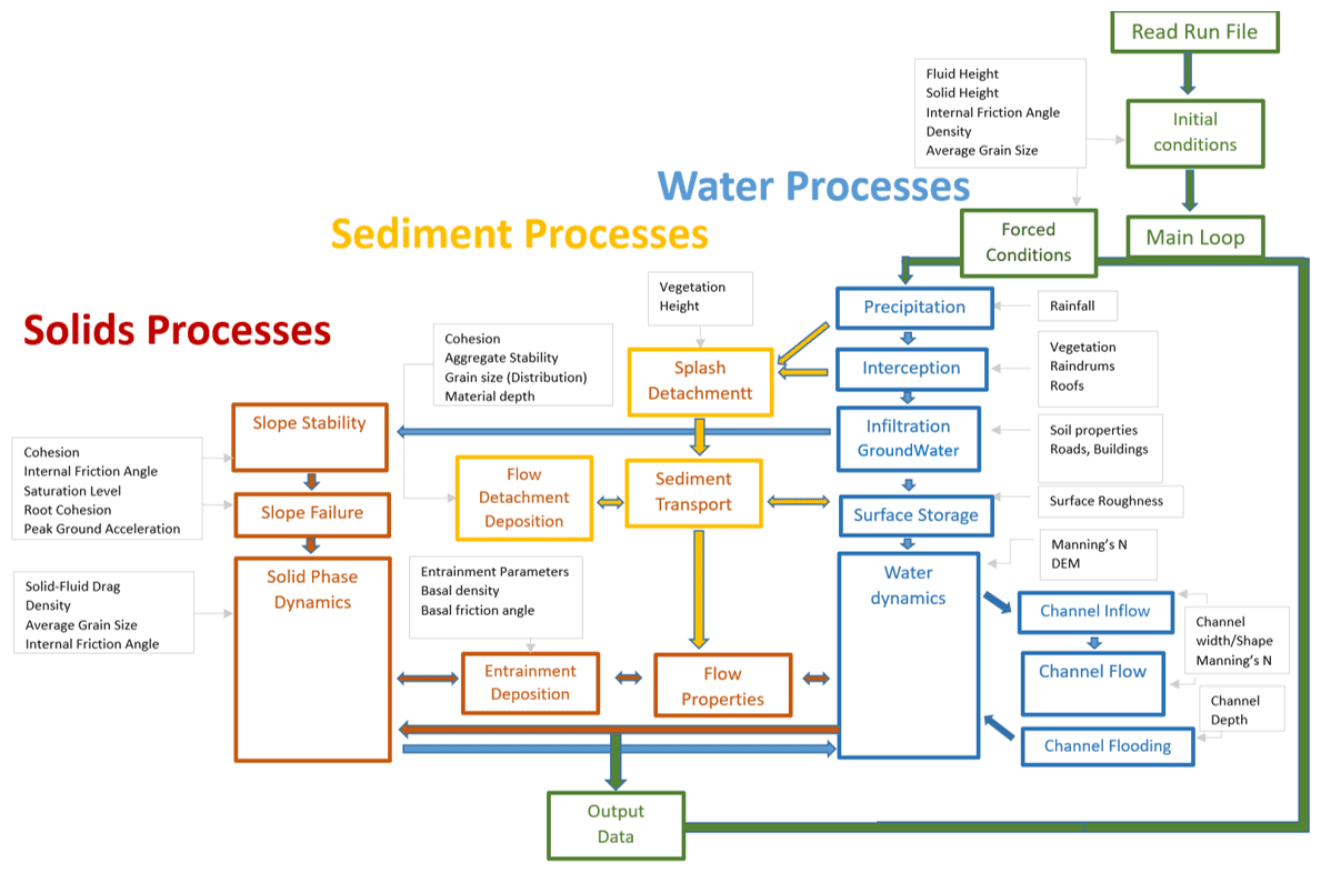
Figure 3 A schematic overview of the OpenLISEM Hazard model, including the link with the most relevant input data.

Similar catchment-integrated simulations that include hydrology, entrainment, and debris flow initiation have been used successfully by the EDDA model (Chen and Zhang, 2015; Hu et al. 2016) and by the STREP TRAMM model (Lehmann et al., 2019). These models predict entrainment of slope material or landslide deposits but do not alter the elevation model. By using recent developments in numerical schemes, elevation model changes can be simulated without erroneous feedbacks between terrain and flow. The numerical scheme within the model is based on the monotonic upstream cell-centered scheme (MUSCL) (Van Leer, 1979). This scheme uses piecewise linear reconstructions of both the terrain surface and the flow properties. This terrain reconstruction estimates local slope and, in rough terrain, also includes cell boundary elevation differences. Besides shear stress from the bottom surface in a cell, cell boundary barriers can also provide shear resistance to the flow. Our implementation of entrainment therefore takes into account direct and lateral entrainment.

3 Study case

The integrated OpenLISEM multi-hazard model was applied in the Hongchun watershed, located near the town of Yingxiu in the epicentral area of the 2008 Wenchuan earthquake, in Sichuan province, China. This watershed experienced numerous co-seismic landslides and a catastrophic debris flow event in 2010. The debris flow deposits from this watershed dammed the main Min River and flooded the town of Yinxiu (Fig. 4).

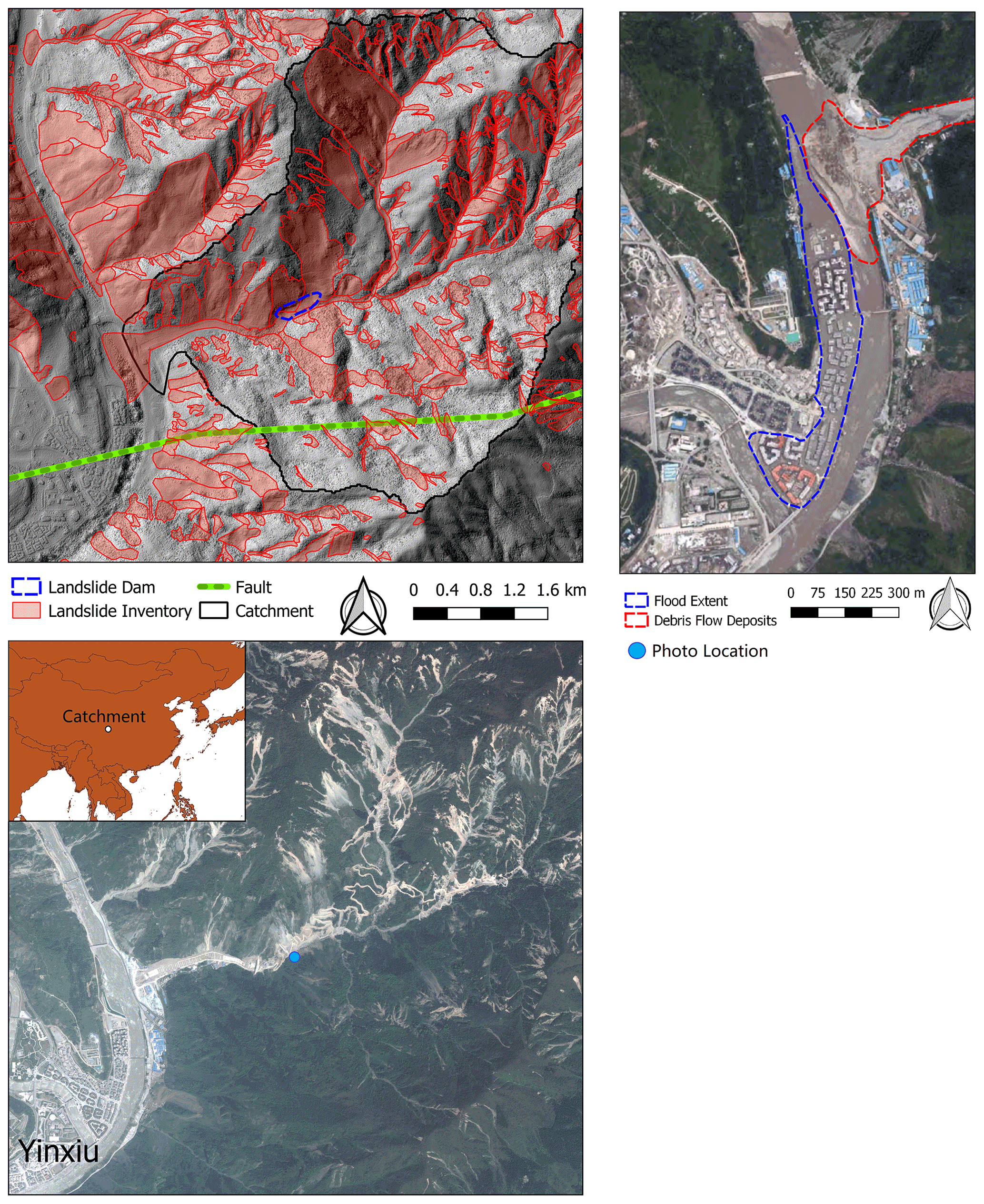
Figure 4 An overview of the Hongchun watershed: (top) hillshade image with co-seismic landslide map from Tang et al. (2016); (bottom) post-event natural color composite from the Pléiades satellite showing the situation in 2017. The construction of massive debris flow mitigation works in the outlet of the watershed is clearly visible, as is the continued mass movement activity 9 years after the earthquake. (Right) Aerial image of the 2010 debris flow blocking the Min River and causing flooding in the town of Yinxiu. Top-right imagery from PLEIADES ©CNES 2010, distribution Airbus DS, and bottom imagery from PLEIADES ©CNES 2017, distribution Airbus DS.

This watershed has an area of 5.3 km², and elevation ranges between 900 and 1700 m. The very steep slopes of this watershed (>30^∘ slope for more than 86 % of the catchment) were covered by dense forests before the earthquake in 2008. The steep terrain and sharply incised channels provide few locations for human settlements. The touristic town of Yinxiu is located adjacent to the Min River and opposite of the outlet of the Hongchun watershed. The lithology of the area consists mainly of highly fractured granitic rocks, with some pyroclastic rocks, limestones, and sandstones (Tang et al., 2011). The texture of the weathered material is predominantly clay loam with large amounts of gravel. The Beichuan thrust fault runs straight through the watershed (Fig. 4; Mahodja et al., 2016). In 2008, the fault was ruptured in the Wenchuan earthquake (M_w7.9). After the earthquake, numerous landslides occurred in the area, leaving large volumes of deposits in the streams and channels and removing the vegetation from 50 % of the area. A detailed co-seismic landslide inventory from Tang et al. (2016) is shown in Fig. 4. The northern part of the catchment, which is part of the hanging wall, was more impacted than the southern part. One of the largest landslides in the watershed blocked the main channel of the Hongchun catchment (Fig. 4), with the deposits exceeding 8 m in depth and 70 m in width.

3.1 The multi-hazard event of 2010

In 2010, 2 years after the earthquake the area experienced several rainy weeks followed by a high-intensity rainfall event. This event consisted of two peaks of several hours of rainfall, with intensities up to 33 and 31 mm h⁻¹ and a total event duration of 15 h. In total, 220 mm of rainfall fell in the two days surrounding the event.

During this event, a debris flow was generated by entrainment of loose landslide deposits, and the landslide dam located in the central channel was breached. Due to the dam breaching, the volume of the flow increased substantially, also due to more entrainment downstream. Upon leaving the Hongchun watershed, the debris flow material deposited in the Min River, with a thickness of up to 15 m high and an estimated total volume of 7.11×10⁵ m³ (Tang et al., 2011). The Min River, which experienced a high discharge at this moment, was diverted laterally and flooded parts of the nearby newly reconstructed the town of Yinxiu (Fig. 6). For a more detailed description of the event, see also Tang et al. (2011) and Ouyang et al. (2015). A schematic overview of the event is provided in Fig. 5.

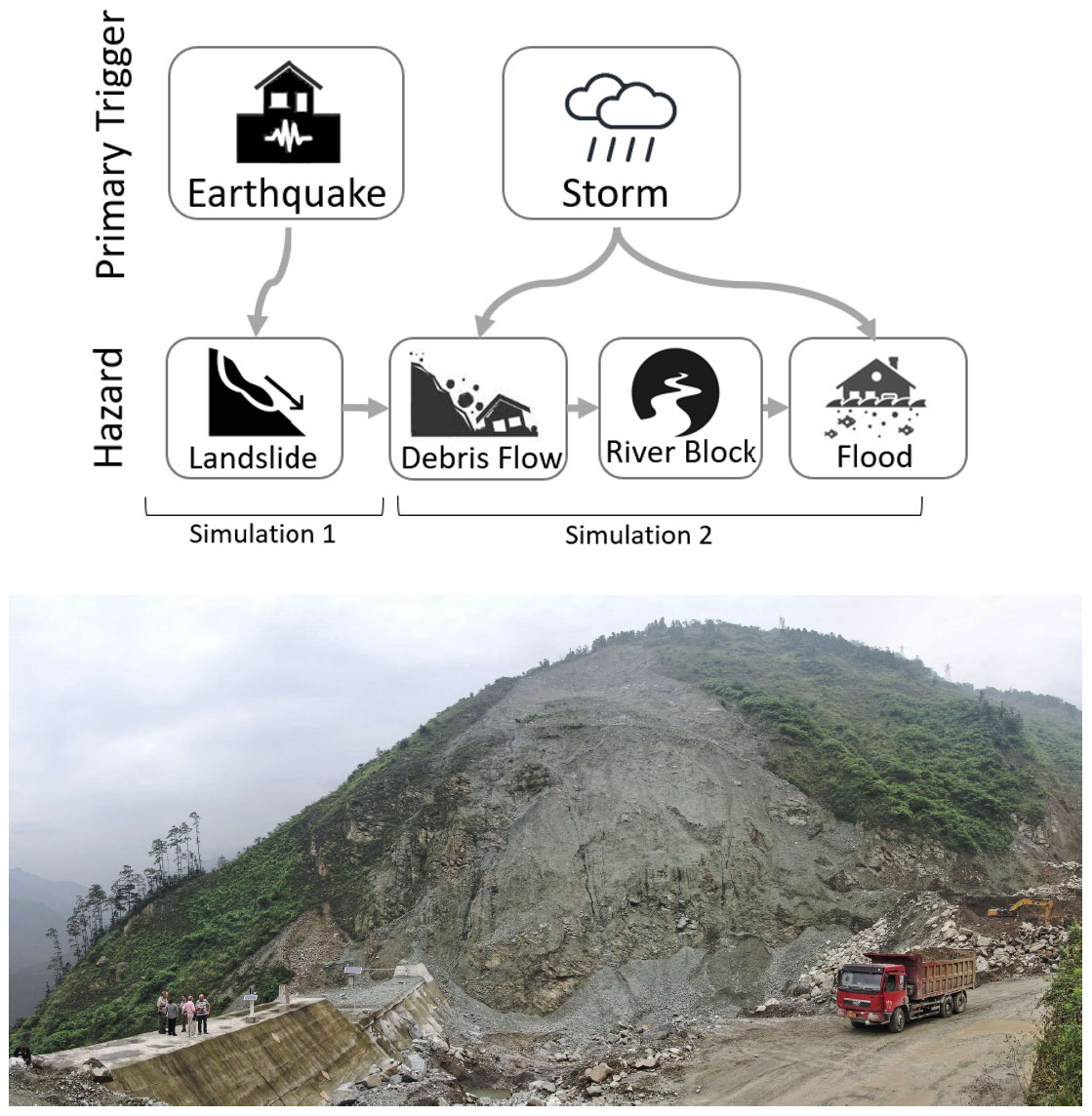
Figure 5 (Top) A schematic overview of the stages of the described event. The events for simulation 1 occurred directly after the earthquake in 2008. The events for simulation 2 occurred after the rainfall event in 2010. (Bottom) A view of the situation at the landslide dam in 2014 (as indicated in Fig. 4, photo taken from the south side of the main gully). From https://www.mergili.at/ (last access: 31 August 2022) with permission from author.

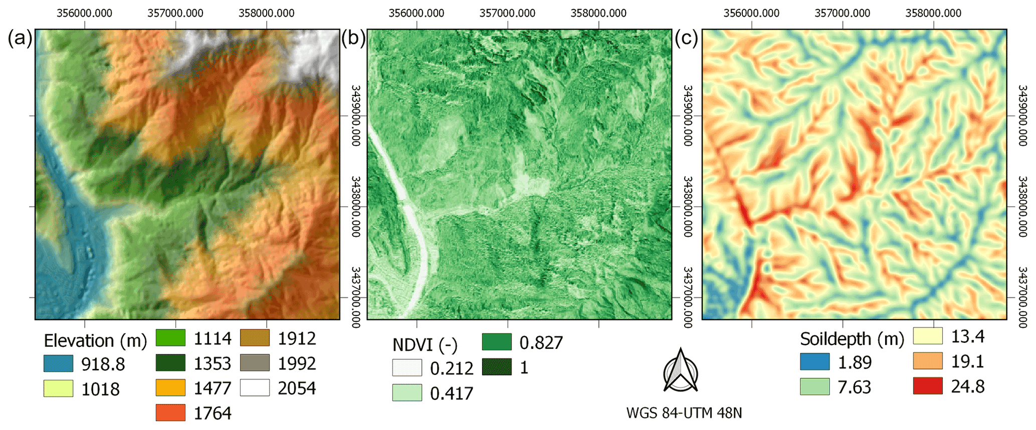
Figure 6 An overview of the input data for the first-stage simulation in Hongchun catchment: elevation model (a), NDVI (b), and modeled soil depth (c).

In summary, the study area experienced two different multi-hazard chains that will be simulated.

• Co-seismic chain. The first one was experienced during the earthquake, when ground shaking and topographic amplification triggered a series of co-seismic landslides, some of which blocked the Hongchun stream.

• Post-earthquake chain. Heavy rainfall triggered debris flows due to entrainment, which broke the co-seismic landslide dam. The resulting debris flow dammed the Min River, which was diverted into the town of Yingxiu.

All simulations include entrainment of estimated soil depth, hydrology, and the related surface processes as described in the theory section.

3.2 Model input and parameters

The input data are based on a combination of laboratory or field measurements and drone- or satellite-based spatial data products (Table 1).

Table 1 List of input data and sources for the multi-stage multi-hazard modeling with OpenLISEM Hazard.

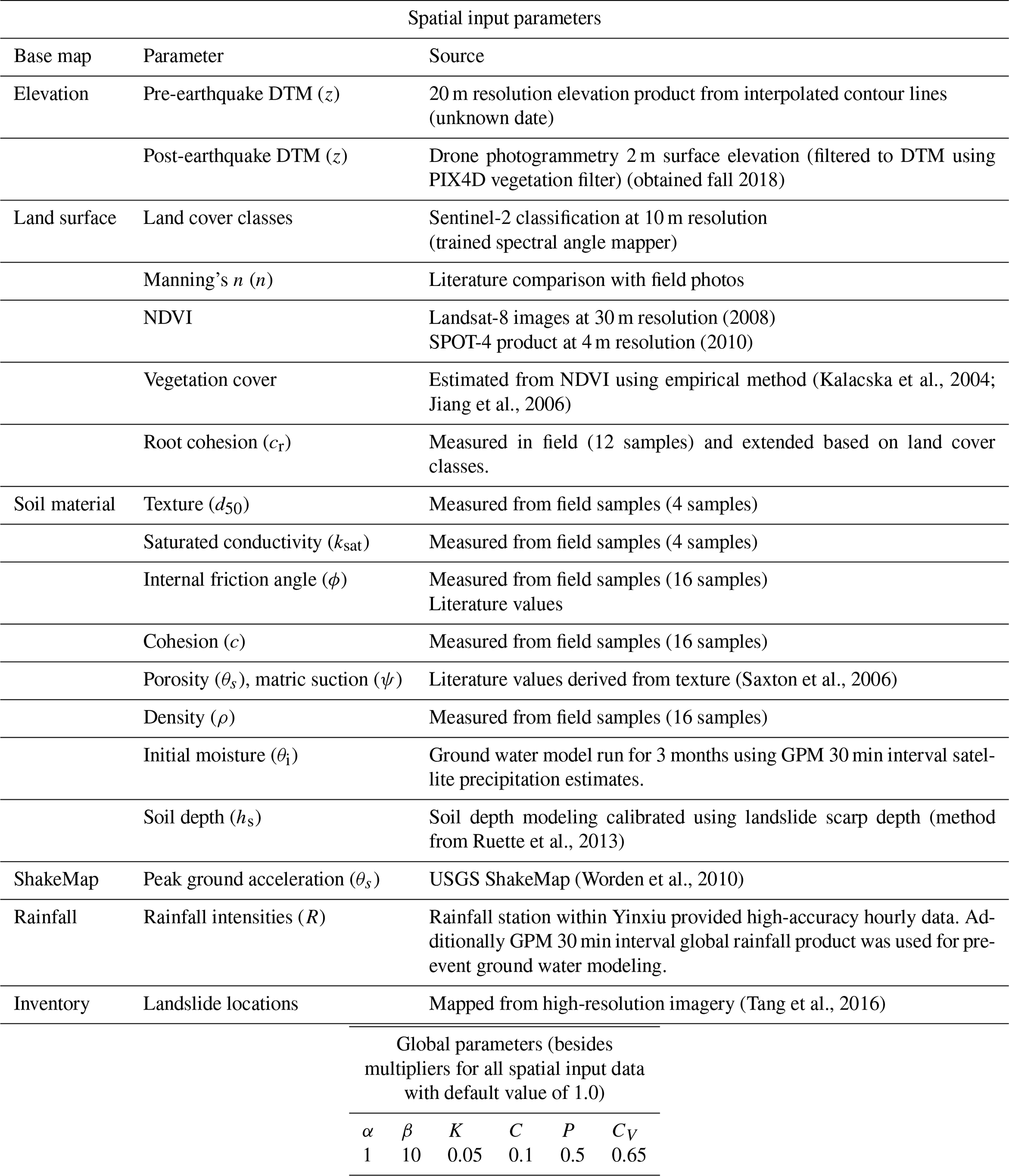
A pre-earthquake digital terrain model with 20 m spatial resolution was obtained from the local government. Unfortunately, we were not able to obtain better-quality pre-earthquake elevation data. Because of this a comparison of the pre-earthquake contour lines with post-earthquake elevation does not yield useful data. Post-earthquake surface elevation data were available at 2 m spatial resolution, acquired from fixed-wing drone flights (see Fig. 6) and filtered using the Pix4D digital terrain model (DTM) filter to remove vegetation (Pix4D, 2017). Flow simulations typically are most dependent on the accuracy and spatial resolution of the elevation model. In order to have an effective compromise between detail and computation time, we resampled all input base maps to the final resolution of 10 m, at which the simulations were carried out.

Pre-earthquake normalized difference vegetation index (NDVI) values were calculated at 30 m resolution Landsat-8 images from 2008. A post-earthquake NDVI map was obtained from 4 m spatial resolution SPOT images acquired in 2009. NDVI values were used to estimate leaf area index (LAI) by applying an empirical relation obtained from tropical forest data (Kalacska et al., 2004). We used it to estimate fractional vegetation cover using a similar empirical relationships (Jiang et al., 2006).

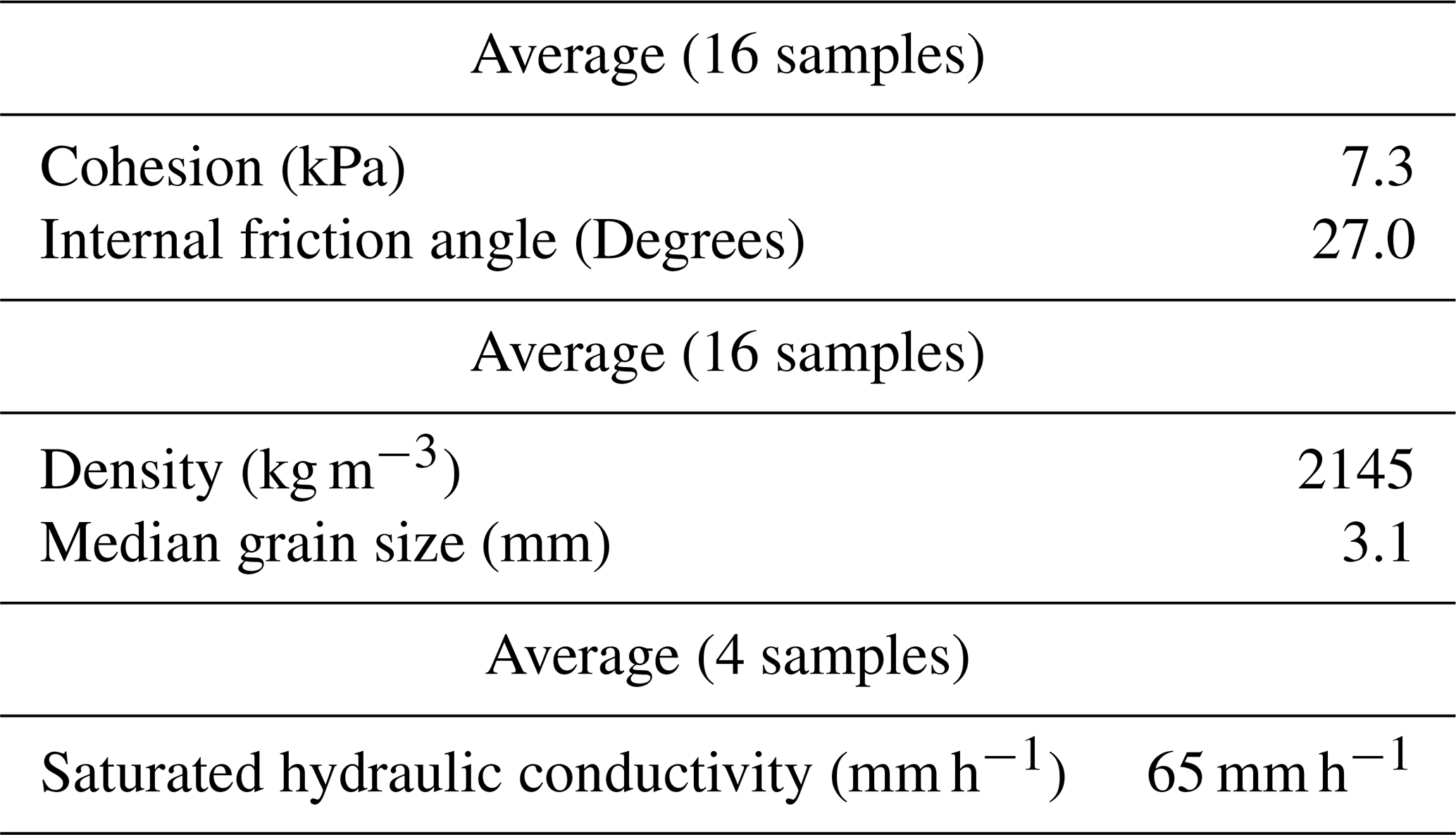
Spatial seismic acceleration data were obtained from the USGS ShakeMap product (Worden et al., 2010), developed using combinations of measurements and intensity prediction equations, and peak ground acceleration (PGA) values were around 1.5 g for this earthquake in the Hongchun area. The PGA value reflects estimated surface shaking but does not take into account the complex variability in site effects such as amplification due to soil or topography. Landslide material strength parameters were obtained from triaxial strength tests performed for engineering reports ordered by the local government (Table 2; Yang, 2010; Hao et al., 2011; Li et al., 2011b). The consolidated drained triaxial tests were performed on samples acquired from both the deposition and source areas, although exact locations are unknown. The resulting average values for cohesion of 7.3 kPa and internal friction angle of 27^∘ were calculated from 16 samples. While the cohesion and density match the values found in other studies (Ouyang et al., 2015; Domenech et al., 2019), the internal friction angle was estimated to be between 30 and 40^∘ in a previous study (Ouyang et al., 2015), based on measurements of internal friction angle on similar igneous rocks in the nearby Xiaojigou ravine. The difference between these values can be explained by the material used in the triaxial tests. In our case, material from landslide depositional areas or areas close to a landslide source was used. These samples contain more fractured and loosened material. Thus, these measurements will provide a more appropriate value in post-earthquake entrainment simulations. The root cohesion is not used for slope stability in the model as roots do not reach the depth of the typical failure plane. Instead, the root cohesion is used to increase shear strength for the entrainment prediction. Here, vegetation cover influences the predicted erosion. However, for pre-earthquake slope stability estimations, a value of 35 ^∘ was used, as was done in other studies (Ouyang et al., 2015; Domenech et al., 2019). Textures were found to be clay loam with large amounts of gravel. Saturated infiltration rates were measured in the field by using field ring infiltration tests. Because of the large amounts of gravel and macro-pores within the materials structure, infiltration values were relatively high. Values were obtained for a total of four locations, which gave an average value of 65 mm h⁻¹ for saturated conductivity. Other soil-related parameters such as porosity, density, and matric suction were obtained using the pedo-transfer functions from Saxton et al. (2006).

Table 2 Strength parameters for the debris flow material in the Hongchun catchment (Yang, 2010; Hao et al., 2011; Li et al., 2011b) and saturated hydraulic conductivity.

Soil depth values were obtained by applying the spatial soil depth model from Ruette et al. (2013), which uses steady-state assumptions to balance material production with soil movement according to an empirical formulation of erosion and lateral transport. The production of weathered material depends on the weathering rate of bedrock. Since weathering rates are generally difficult to obtain, this parameter becomes the main calibration parameter. Validation was done using soil depth values obtained from landslide scarps. In this study, we used the pre- and post-earthquake elevation model differences provided by Tang et al. (2019). From their data, we sampled elevation model differences in landslide source areas to obtain failure depths, assuming that the failures were at least as deep as the top layer of weathered material. In the case of shallow landslides, we took the maximum landslide depth as soil depth. For the larger, deep-seated landslides, no samples were taken since it was not possible to obtain a good estimate of the depth of the top layer. Additionally, we simulated a second layer within the slope stability calculations with an additional depth of 20 m to capture any deeper rotational slides within the bedrock material. We assumed that this second layer did not contain groundwater, had an internal friction angle of 35^∘, was subject to subsurface lateral forcing, and was influenced by the weight of the upper layer. Calibration results and cumulative distributions of depth values are shown in Fig. 7.

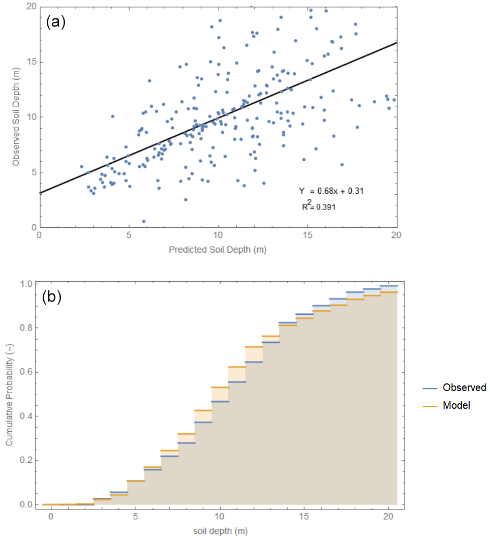
Figure 7 Soil depth simulation results. (a) A comparison of predicted vs. observed values. (b) Probability distribution for observed and simulated soil depth values.

The effect of vegetation on slope stability and entrainment rates were taken into account by adding root cohesion. The recovery of vegetation in the landslide-affected areas developed through distinct stages (Huang et al., 2017). We estimated the average root cohesion for the various vegetation classes using a combination of literature data and measurements (Schmidt et al., 2001; De Baets et al., 2008; Chok et al., 2015). We used the method as described by De Baets et al. (2008) which requires measuring root critical force and root diameters for all significant roots within a specific surface area. Then, after converting force to tensile strength, the total effect of the roots per unit area can be estimated using Eq. (40).

$$\begin{array}{}\text{(40)}& c_{\mathrm{root}}={\displaystyle \frac{\sum T_i{n}_i{a}_i}{A}}\left(\sin \left(\mathit{\theta }\right)+\cos \left(\mathit{\theta }\right)\tan \left(\mathit{\varphi }\right)\right),\end{array}$$

where  c_root is the added apparent root cohesive strength (kPa), i is the root diameter class, T_i is the root tensile strength (kPa), n_i number of roots within the diameter class, a_i is the cross-sectional area of the root, A is the area of the soil occupied by roots (m²), θ is the angle of shear distortion in the shear zone (^∘), and ϕ is the internal friction angle (^∘). Note that the term related to the shearing angle (sin (θ)+cos (θ)tan (ϕ)) is usually assumed to be approximately 1.2 (Baets et al., 2008). Here, we used a spatial calculation of this variable.

A total of 12 measurements of root cohesion averaged over a 0.1 m² area were done. On average, 108 roots were found per test site of 0.1 m², with an average diameter of 3.6 mm. Average values for young, post-landslide vegetation were found to be 4.8 kPa, and averages for medium-sized vegetation were found to be 6.2 kPa. For mixed forest, literature values were used, and root cohesion was estimated to have a value of 8 kPa (Chok et al., 2015; Huang et al., 2017). For each land cover class, the root cohesion from the closest measured vegetation type was used. Finally, within each land cover class, we linearly scaled the root cohesion to fractional vegetation cover values that were derived from the NDVI both before and after the earthquake.

3.3 Calibration and validation

The predicted co-seismic failure areas were calibrated using the landslide inventory and mapped deposition based on aerial imagery and pre- and post-event elevation data differences. Within the inventory, no separation between source and deposit areas was provided. Therefore we assumed that, based on field visits, on average the 25 % highest part of each landslide polygon represented the source area. In order to compare the outputs of our model with others, we parameterized two other regional slope stability models. The first of these is Scoops3D, which uses random spheroid sampling to find the landslides with the lowest failure volumes and lowest factors of safety for each pixel (Reid et al., 2015). This model can also use seismic shake maps as input. The second model is r.slope.stability, which uses random ellipsoid sampling to find the lowest factor of safety and failure depth for each pixel (Mergili et al., 2014). The version of the model that was used did not incorporate seismic acceleration, so the output is calibrated without addition of seismic forcing. Recent developments of this software have added these effects. The Newmark displacement method (Newmark, 1965) was not used in our comparison. The primary reasons were the lack of predicted failure depths and the high similarity to the infinite slope model. When the critical acceleration is taken as threshold and failures occur when accelerations go beyond this value, results are identical to an infinite slope model that incorporates seismic acceleration. For both Scoops3D and r.slope.stability, the subsurface description is identical to the input for OpenLISEM Hazard. As a measure of model fit, we used Cohen's kappa value. This metric has benefits over simple accuracy, especially for modeling landslide occurrence, since it compensates for the large amounts of true negative predictions (no landslide in model and inventory) that usually dominate landslide study sites (Bout et al., 2018).

The second phase of the modeling first simulates hydrology and a debris flow initiated by entrainment. Then, within the same simulation, the Min River is blocked by debris flow material, and the town of Yinxiu is flooded. Calibration for this part of the modeling is based on mapped deposition extent in the Min River, the flood extent in the town of Yinxiu, and the estimated depositional volume (approximately 7.11×10⁵ m³).

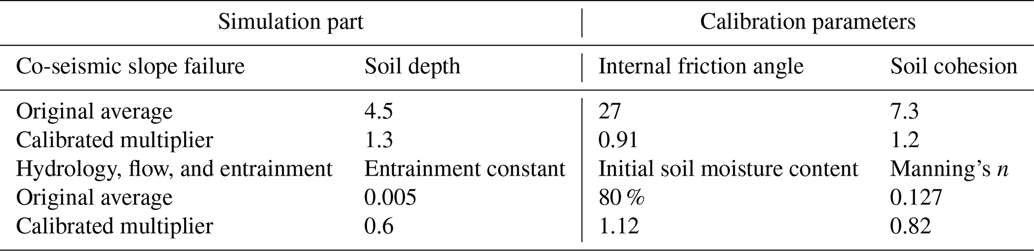
Calibration of the entrainment and debris flow runout was based on the final spatial deposit extent at the catchment outlet. The calibration parameters for each part of the simulation are shown in Table 3. An exception to this was the entrainment constant, for which no clear guideline was known to determine the value for specific terrain types. Based on earlier simulations and flume tests from Takahashi et al. (1992), a starting value was chosen of 0.05. For initial soil moisture content, the value is cut off at full saturation. Initially, each parameter was varied by choosing values between 60 % and 140 % of the original value. After initial calibration was done, the parameters were adjusted according to the steepest descent principle in order to find the best set of parameter values. To have a level of validation in the simulations, the parameters resulting from calibration of the first chain were used as input for the second chain.

Table 3 Calibration parameters, their initial values, and their final calibrated values for both chains.

4 Results

Simulation results for the first chain, co-seismic slope failure and runout, are shown in Figs. 8 and 9. Both the accuracies and Cohen's kappa values for each of the slope stability models used are shown in Table 8.

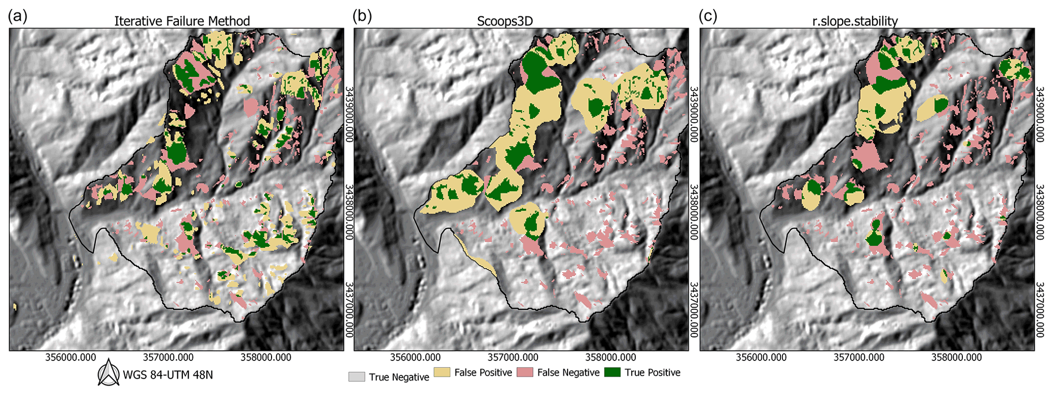
Figure 8 A comparison of simulated slope failure extent with mapped co-seismic slope failures. (a) OpenLISEM Hazard iterative failure with subsurface forcing, (b) Scoops3D random spheroid sampling, and (c) r.slope.stability random ellipsoid sampling.

Figure 9 (a) Initiation depth from the slope failure simulation. (b) The simulated final deposit depth of the landslides. Blockage location shown with blue outline (mapped landslide dam). (c) A comparison of modeled landslide runout with the mapped landslide inventory. (d) Maximum landslide runout flow depth.

Table 4 Slope stability simulation accuracy and Cohen's kappa values.

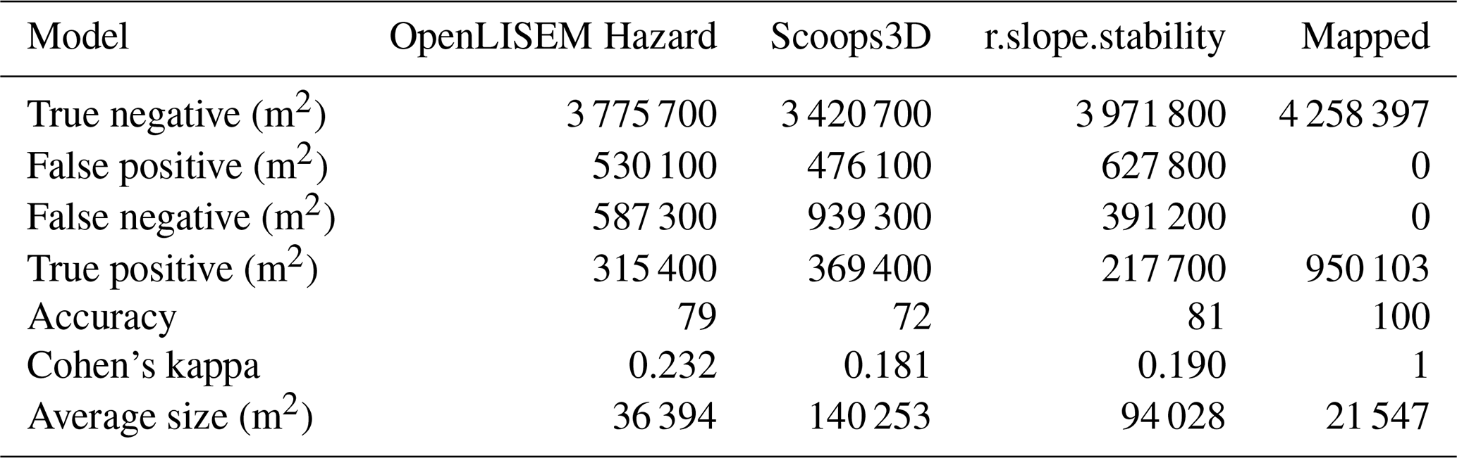
The general spatial patterns are predicted reasonably by all models, but the models differ considerably in details. For the ellipsoid and spheroid sampling done by r.slope.stability and Scoops3D, the failures are larger than those actually mapped (Table 4). For the iterative method, sizes are mixed but much more similar. Major landslides, in particular in the north, are predicted with similar size, although not in the exact location, by all models. The highest accuracy (81 %) is obtained using r.slope.stability and the highest Cohen's kappa (0.232) value with OpenLISEM Hazard. The OpenLISEM Hazard iterative method shows the best reproduction of the general pattern, in particular since both Scoops3D and r.slope.stability lack slope failures in the southern half of the catchment. Of the three models, r.slope.stabiltiy and OpenLISEM Hazard show similarity in total failure area when compared to the inventory. Despite the achievements of the model, errors remain large, and Cohen's kappa values indicate all models have low to moderate reliability.

4.1 Runout and the blocking of the Hongchun stream

When slope failures are simulated, OpenLISEM Hazard automatically introduces landslide runout by transferring the failed volume and its properties to the Mohr–Coulomb solid–fluid mixture flow equations. The depth of slope failures determine directly the amount of solids and fluids introduced (Fig. 9D). The landslide material moved down the slopes into the main channel of the Hongchun watershed, blocking it in at least one location (Fig. 9A). The accuracy for the calibrated simulation was 64 % with a Cohen's kappa value of 0.28 (Table 5), which is mainly attributed to the accuracy of the failures that started this process (Fig. 9B). Runout distances are similar to those mapped, indicated by the landslides reaching the main channels within the Hongchun catchment but not reaching the Min River. In one location the channel was blocked by a deposit 12 to 18 m deep which was simulated with high accuracy as compared to the mapped blockage (Fig. 9B). Engineering reports indicate a similar depth (16 m) for the landslide dam (Yang et al., 2010; Hao et al., 2011; Li et al., 2011b). We considered using the landslide initiation polygons from the inventory to increase the accuracy of the runout simulation. However, since the aim of this research is to provide a true multi-stage modeling setup, we used the integrated prediction of slope failures as input in the runout modeling.

Table 5 Confusion matrix for the landslide runout prediction in Hongchun watershed.

4.2 Validation of failure and runout for the major central landslide using elevation model differences

Two large landslides occurred in the northern part of Hongchun catchment. One of those, near the center of the area, blocked the main channel of the catchment. For this landslide, pre- and post-earthquake elevation models from lidar data are available (Tang et al., 2019), which were used to calculate the landslide volume. For this particular area, we compared the predicted elevation model differences based on slope failure and deposition from our modeling chain with the results from the lidar DEMs (Fig. 10).

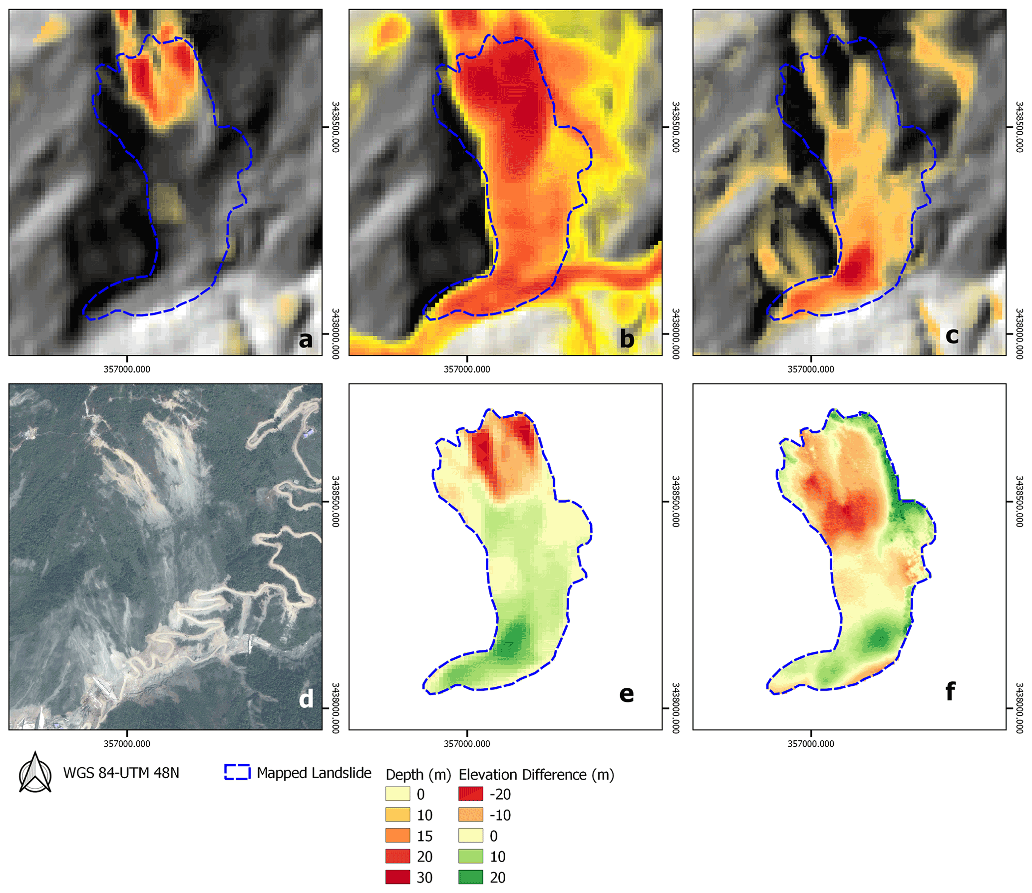
Figure 10 An overview of the largest central landslide in the Hongchun watershed. (a) The simulated failure depth. (b) The simulated maximum runout depth. (c) The simulated deposition depth. (d) Post-earthquake satellite image (Worldview, 2011). Note the mining activities in the landslide deposit area (e) Predicted elevation model differences due to co-seismic landslides. (f) Observed elevation model differences from pre- and post-earthquake lidar data.

Both the slope failure and runout thicknesses are predicted with high accuracy for this landslide. The landslide deposits of around 20 m thickness remained in the main channel without spreading significantly. These deposits have later been mined as materials for local construction. As can be seen in Fig. 10 the failure, deposition, and elevation differences are highly similar with matching spatial patterns.

4.3 Simulation of the second multi-hazard chain

The results from the modeling of the second stage show a full physically based simulation that reproduces the behavior and the impact of the event (Fig. 11). This rainfall event with two distinct peaks resulted in a rainfall amount of 220 mm in 2 d, which was modeled in time steps of 0.5 s. Due to the large rainfall volume, runoff increased rapidly leading to large amounts of sediments that were entrained from the co-seismic landslide deposits. Within the simulation, entrainment takes place after runoff has been converted into streams. There, higher water pressures and velocities provide shear stress on the surface that is sufficient to overcome the materials internal stability. Near the outlet of the watershed, entrainment decreased due to a decrease in slope steepness. This decreased flow velocities but also increased the internal stability of the available material. Because of this, entrainment stopped, the flowing material lost momentum, and it was finally deposited in the Min River.

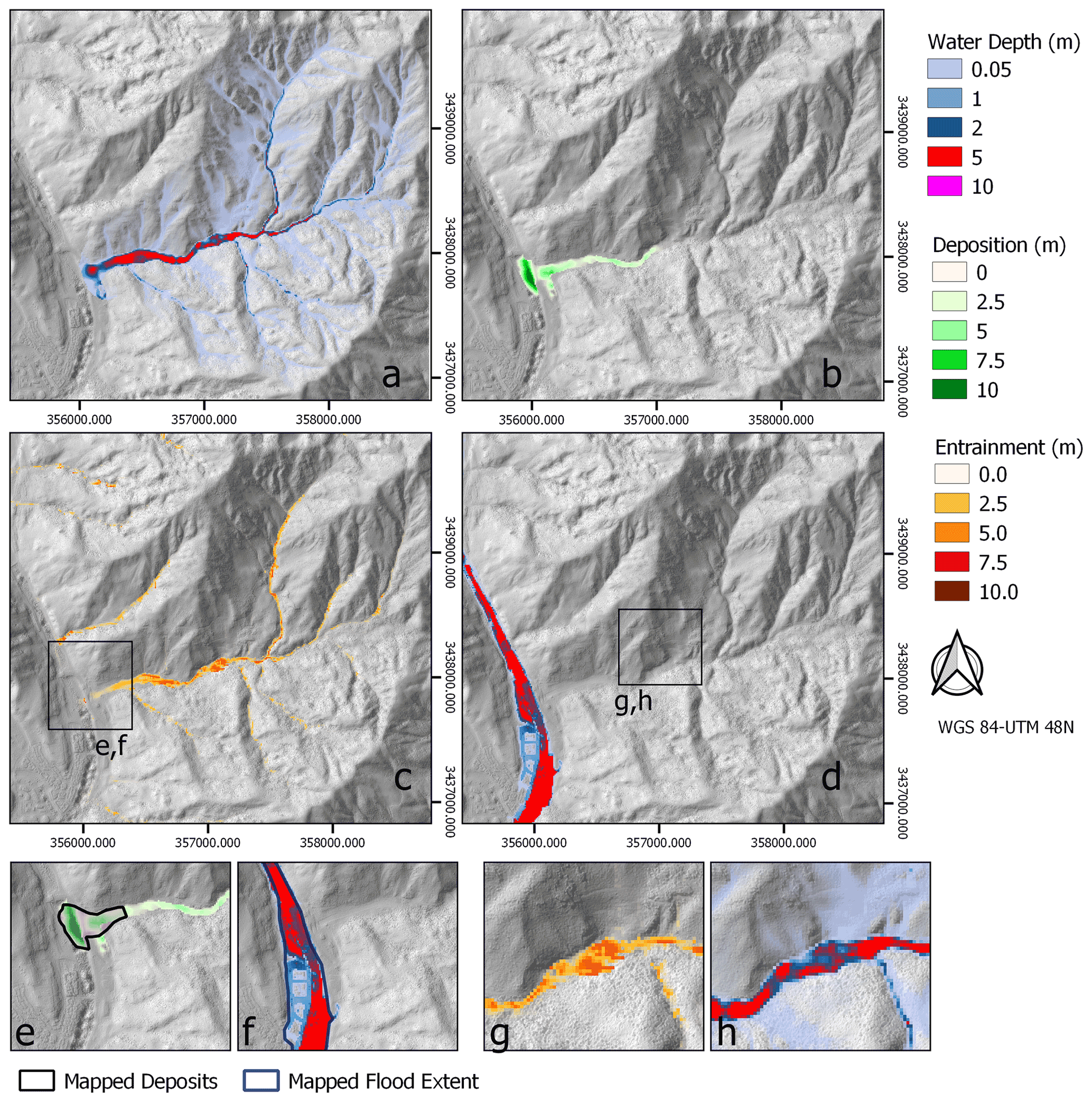
Figure 11 Calibrated simulation results for the second chain in the Hongchun watershed. (A) Maximum total flow depth. (B) Final deposit depth. (C) Entrainment depth. (D) River flood depth. (E, F) Zoom of Hongchun outlet with (E) deposition depth compared with mapped extent and (F) river flood depth compared to mapped flood extent. (G, H) Zoom of Hongchun landslide dam with (G) entrainment depth and (H) maximum flow depth.

Table 6 Confusion matrix, accuracy, and Cohen's kappa values for the debris flow deposition and flooding of the Min River.

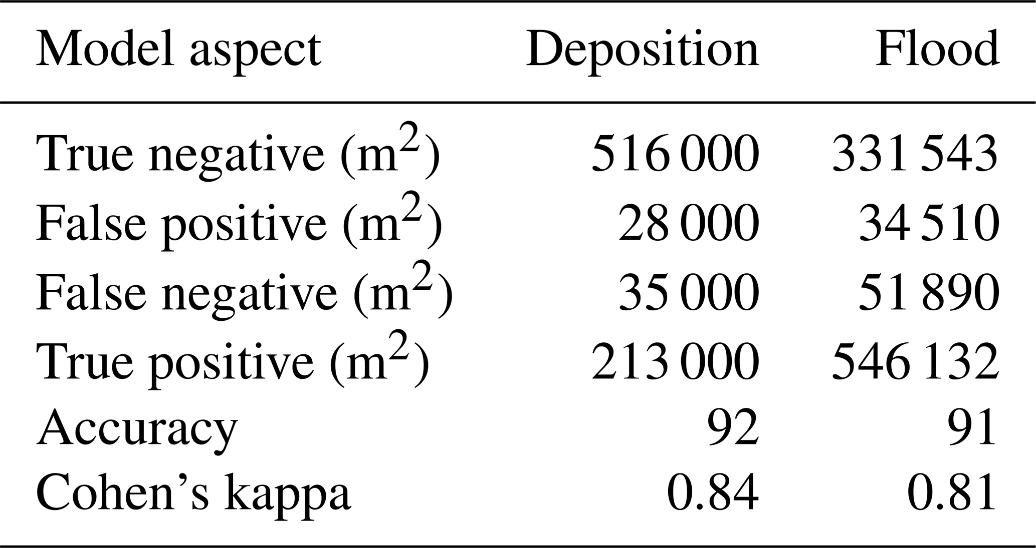
The simulated debris flow reaches the Min River, and the deposits accumulate in the river. Most of the momentum has been lost before the material leaves the Hongchun watershed, and even though the Min River has a velocity of 7 m s⁻¹, the deposited volume is too large to be eroded by the Min River. Both the total deposit volume in the river and the extent of the deposits compare well to the measured and mapped values. The deposits were modeled with an accuracy of 92 % and a Cohen's kappa value of 0.84 (Table 6). The modeled deposited volume is 5.82×10⁵ m³ (the observed estimation of the deposited volume is 7.11×10⁵ m³).

As a final stage of the event, the model predicted the flood behavior in the town of Yinxiu by the Min River as its main course was blocked by the debris flow deposits. The modeled damming area correlates well with the observed deposit volumes and flood extents, obtained from the interpretation of aerial images and field photos from the event (Fig. 14). The flood accuracy is 91 % with a Cohen's kappa value of 0.81 (Table 6). Since the elevation data were upscaled from 2 m resolution to 10 m, the multi-story buildings merged with small streets to become a joined obstacle for the flow, which corresponds with the visual observations.

While validation using comparison to mapped extent is a useful tool, it does not guarantee all aspects of the hazard are correctly simulated (e.g., timing, velocities, heights). While a model might have correctly predicted the extent of impact, it might predict the occurrence too early or late, with incorrect velocities or flow heights. While we do not have data on flow heights or velocities, we confirmed with local authorities the debris flow was reported at 03:30 LT (Sichuan local time, GMT + 8 h). In our simulation, the first peak of solid material at the outlet occurs at this time (Fig. 12). The major peak of debris material occurs later, at 06:00 LT, but we could not confirm in the town of Yinxiu for how long the debris kept arriving at the Min River.

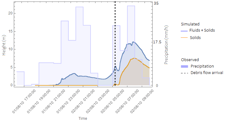
Figure 12 Time series data for rainfall, total flow height, and solid flow height at the Hongchun outlet. Reported debris flow occurrence time is indicated as “debris flow”.

5 Discussion

5.1 Uncertainties in modeling the multi-hazard chains

Several major obstacles in the simulation of co-seismic landslide occurrence can be identified, which are related to the assumptions and techniques used in the models. The iterative method that is implemented in OpenLISEM Hazard assumes that, at least initially, failure surfaces are parallel to the terrain surface. This assumption can lead to a variety of issues when the terrain has small-scale variations that do not represent the overall topography. This assumption is not present in the random ellipsoid sampling methods. The iterative method shows similar failure depths and locations but generally separates slope failures more, whereas the other models show larger joined failures. The predominant cause of this behavior most likely lies in the subsurface force iteration, where the potential failure surface is also initially assumed to be parallel to the surface. Then, when an obstacle exists that alters the slope around several pixels, the subsurface forces are blocked, and potentially larger failures become disconnected (Fig. 13).

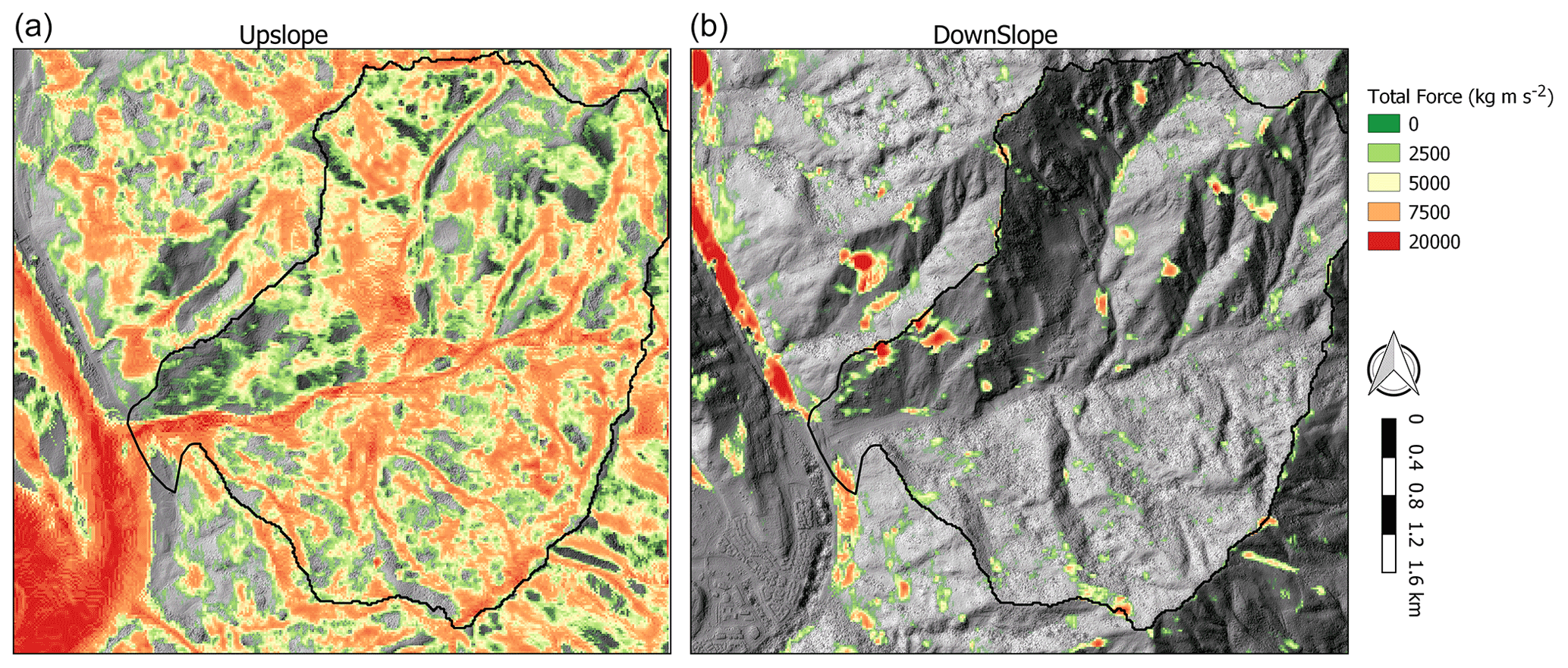
Figure 13 The upslope (a) and downslope (b) additional forcing that is estimated based on an iterative solution for subsurface force redistribution.

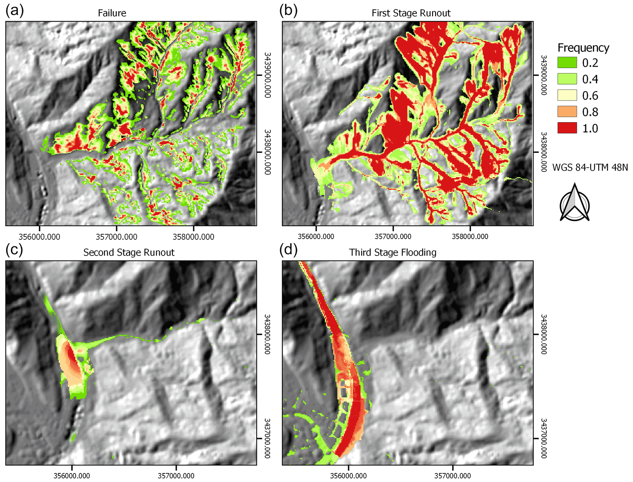
Figure 14 Ensemble simulation results for the Hongchun watershed. Visualized is the normalized probability, based on the ensemble of runs with varying input parameters, of the hazard occurring at each location. (A) Co-seismic slope failure. (B) Co-seismic landslide runout. (C) Post-seismic debris flow deposition. (D) Post-seismic river flooding due to blockage.

Secondly, structural geological input data are not available and cannot be used in the iterative method. For three-dimensional analysis using random ellipsoid sampling, structural weaknesses could be implemented by altering strength properties of specific layers. When such data are available, applications of the detailed random ellipsoid sampling method can allow for a greater predictive value (Mergili et al., 2014; Cance et al., 2017; Tun et al., 2019).

Furthermore, seismic acceleration of material is a complex and dynamic process, driven by seismic waves compressing and stretching the sloping materials. Such waves reflect and refract based on material properties and boundary conditions, which leads to a variety of topography or material-based amplifications. These amplifications are generally important in landslide hazard modeling (Jafarzadeh et al., 2015). However, shake maps produced by the USGS utilize empirical predictive functions to spatially extend ground accelerations and ignore these crucial local amplification effects. As a result there is high spatial uncertainty in the peak ground acceleration values we have used as input. Such uncertainties can be overcome by linking slope stability approaches to seismic wave modeling, a computationally heavy task that has of yet not been performed for the Wenchuan earthquake.

The final calibrated values of the input parameters were within a reasonable range (between 50 % and 150 %) with respect to the original estimated ones. Two parameters stood out significantly in the calibration process. The first of these, soil depth, is a crucial parameter as it determines the amount of material that is released, which is of direct influence in the runout modeling. This can indirectly influence the amount of material available for entrainment by flow at a later stage. In an active landscape, soil depth patterns are determined by rock weathering rates and mass transport/wasting. Soil depth increases until there is sufficient material to induce slope failures or significant erosion. As a result, at many locations, combinations of soil depth and slope can be near a critical state. The spatial component of soil depth is therefore of high importance. Despite its importance, soil depth is very difficult to measure over larger areas and has a high uncertainty in most model applications (Kuriakose et al., 2009). Because information on soil depth is difficult to obtain through direct observation or remote sensing, it is generally obtained through modeling approaches (Kuriakose et al., 2009; Ruette et al., 2013). Another reason for the uncertainty in soil depth information is that a soil layer is a theoretical concept that does not always translate well into reality, whereas weathering is a more gradual process. A second variable which was difficult to estimate is the entrainment coefficient. Currently, there are several types of entrainment equations available in the literature, but most of these lack significant guidelines for selecting practical entrainment parameters (Iverson and Ouyang, 2015). Besides this coefficient, other parameters used in the entrainment equations, such as soil cohesion, internal friction angle, and moisture content, were measured in the laboratory and are common values for geotechnical research. However, the number of samples that are tested for these geotechnical parameters are always limited, and their spatial variability is generally high.

5.2 Ensemble simulations

To analyze the uncertainties within the multi-hazard multi-stage modeling setup, we extended the calibration process to an ensemble analysis. In total, for each of the six calibration parameters, three equal-interval values were used (calibrated values), as well as the values plus or minus a given range of 10 %–50 %, as indicated in Table 7. Thus, the first simulation was repeated 27 times. The best estimate was used as input for the second simulation, which was similarly repeated 27 times. In total, 56 simulations were thus performed, out of which normalized frequencies were generated for hazard occurrence. We defined a threshold of 0.25 m above which a flow is counted as an actual hazard occurrence to avoid that the results would include runoff with insignificant depths.

Table 7 Parameter settings for the ensemble simulations.

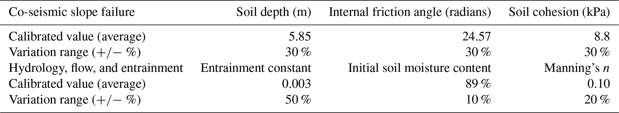
Figure 14 shows an ensemble plot for each stage of the simulation. For each location, these maps show the normalized probability of hazard occurrence within the ensemble of simulations.

The four maps in Fig. 14 illustrate how much the variation of the input parameters influences the simulated hazard for the four stages of the multi-hazard chain. The prediction of co-seismic slope failures shows the highest spread and therefore the highest influence on the total event variability. The uncertainty in the input parameters influences the slope failure equations most since we have simulated the multi-stage event as an integrated sequence in which the uncertainties in one process influence various other processes. Despite the uncertainties, there is a substantial certainty that flooding of the town of Yinxiu will occur, independent of the input parameters. For all performed simulations, the deposition volume in the Min River is never below approximately a third (2.1×10⁵ m³) of the estimated volume (7.11×10⁵ m³). For at least 80 % of the simulations, there is at least some flooding experienced with a depth above 50 cm in Yinxiu. In comparison to other multi-stage hazard studies, these numbers are relatively high (Mergili et al., 2018b). Mergili et al. (2018b) reported that threshold behavior and nonlinear effects dominated the alterations in model behavior with changing parameters. While the event they describe is quite different from the Hongchun disaster, there is a similar influence from threshold effects on the interpretation and certainty of model outcomes. In this current study, threshold effects most likely exist related to the landslide dam behavior in both the Hongchun watershed and the Min River. With altered input, there could be insufficient material for landslide dam creation or not enough flow and entrainment for breaching. However, we do not encounter scenarios that fall below the threshold of breaching in our ensemble.

There are several factors that drive the high likelihood of flooding in the town of Yinxiu. The event is initiated by several triggering conditions, or forcings, such as the seismic acceleration and rainfall, which occur in a very steep watershed and determine the behavior of the hazardous processes. Seismic accelerations during the 2008 earthquake reached the 10th and highest USGS category for seismic acceleration (>139 % g). Similarly, the 2010 rainfall event resulted in 220 mm of accumulated rainfall within 48 h, with significant rainfall in the weeks before. For events with a smaller return period and lower intensity of the triggering process, variability and uncertainty in the potential outcomes might be larger. An example is the occurrence of landslides' long duration through low-intensity rainfall, which is a much larger challenge for physically based modeling (van Beek, 2002). In our case, material strength parameters must deviate significantly from their measured and estimated values in order not to result in slope failure under such extreme seismic acceleration. Thus, the severity of the triggering events causes the simulations to predominantly show major slope failures, debris flows, deposition in the Min River, and finally flooding of the town of Yinxiu.

5.3 Usability

A major challenge for the application of such a type of multi-hazard modeling is the step from back-analyzing past events to forward prediction of future events. In the case of back-analysis, calibration is possible on data from the event itself, whereas predicting future events must be done without knowledge of the hazard that will occur. By calibrating on data of multiple events and validating on other events (checking for accuracy using calibrated input from other events), a more robust model can be established. When validated on similar events, a higher level of confidence can be generated in the abilities of the model to predict future events. In the case of the Hongchun watershed, the accuracy of the presented numerical experiments depended on thorough calibration. This is caused by several factors, such as the uncertainties in the input data and the limited accuracy of the assumptions made within the model equations. In studies where multi-stage multi-hazard events are considered, this becomes even more difficult due to threshold effects and stacking uncertainties (Mergili et al., 2018a). Despite these issues, calibration is possible by performing model runs with a large set of varying input parameters and comparing the output with measured data on the event (e.g., discharge, extent of landslides, debris flows, or floods). Validation options, on the other hand, may be very limited as similar events are very rare. Debris flows occur more frequently within the watershed and can therefore be both calibrated and validated (Domenech et al., 2019). However, the multi-hazard chain as described in this research is a rather unique sequence of events that does not easily allow for validation except when looking at individual components. Even then the co-seismic slope failure and runout stages do not occur frequently within the same region. Thus, we run into two primary issues in the predictive use of multi-stage and multi-hazard modeling. Firstly, the complex modeling has internal uncertainties that propagate, stack and provide a challenge in calibration. Secondly, such events occur with very low frequency (Kappes et al., 2012) and can therefore rarely be further calibrated and validated. Despite the difficulties in the calibration and validation process for multi-hazard multi-stage modeling, we have shown that for the Hongchun watershed, many aspects of the first sequence had a high likelihood despite the uncertainties. This indicates the possible use in predicting future events, especially when ensemble analysis is performed to show the relative spread of model results. However, this is computationally intensive and cannot be carried out over large areas yet.

6 Conclusions

We have investigated the potential for understanding and predicting complex multi-hazard co-seismic process chains. A physically based model is used that allows for the simulation of multi-stage and multi-hazard chain events in mountainous terrain. Catchment-based hydrology was combined with slope stability analysis under seismic acceleration. Entrainment of loose material was implemented to alter both topography and the composition of the flow. The modeling setup is able to fully simulate the behavior and impact of multi-stage and multi-hazard events. The developed model code is available as part of the ongoing development of the open-source OpenLISEM Hazard model (https://lisemmodel.com/, last access: 23 August 2022).

The model was tested in the Hongchun watershed, located near the epicenter of the 2008 Wenchuan earthquake, in two sequences of hazard interactions. The first sequences was the generation of earthquake-induced landslides that resulted in runout of landslide materials and the blockage of a stream channel. The second sequence was the triggering of debris flows by extreme rainfall, resulting in the breaking of the existing landslide dam, and the formation of a debris flow fan in the main river, forcing the river to flood the city on its banks. The modeled slope failures show a reasonable accuracy when compared with the actual landslide inventory. The failure simulation is the least accurate process within the simulation (accuracy 64 %). Improvements in this process might be possible using a higher-quality ground shaking input map that includes topographic amplification and other nonlinear terrain-induced effects. Furthermore, a better spatial estimate of the subsurface structure and the three-dimensional variability of strength parameters could improve the accuracy. However, current techniques for simulation of regional failure volumes are still often not achieving the desired accuracy (Wasowski et al., 2011). Over time, such a type of modeling should be able to translate the modeling of seismic acceleration for many earthquake scenarios into a probabilistic earthquake-induced landslide hazard map.

The runout of the co-seismic landslides and the debris flow that was triggered 2 years later were predicted with high accuracy. Pre- and post-earthquake elevation model differences were used to validate the modeling outcomes spatially for the largest central landslide, where high-accuracy elevations models were available for both pre- and post-earthquake periods. In particular, the blocking of the Hongchun stream by co-seismic landslide runout was simulated with good agreement (accuracy 91 %). During the simulation of the 2010 rainfall event, a debris flow was initiated by entrainment, and the landslide dam was breached. Eventually, the model simulated with relatively high accuracy the flood behavior in the second stage of the event (accuracy 92 %).

The sensitivity of the model was further analyzed by looking at ensemble simulation results. Uncertainty propagated through the different stages of the simulations. Despite this uncertainty, the ensemble models showed a high likelihood of flooding in Yinxiu. The model results show high certainty due to both the magnitude of the seismic accelerations, rainfall intensities, and the equations guiding the gravitational flows. This does not mean that the model is able to predict future events with equal reliability. However, it does indicate that, when the inherent uncertainties are taken into account, predictions from advanced spatially distributed and physically based models can provide insight and have some predictive value. Simulation results should be treated with caution. However, with validation and advancements in the understanding of the physical processes, multi-stage multi-hazard modeling might become a useful and trusted tool for decision makers in multi-hazard risk assessment.

Appendix A

Table A1 Parameter list.

Table A2 Continued.