the Creative Commons Attribution 4.0 License.
the Creative Commons Attribution 4.0 License.
 | 02 Sep 2022
Comprehensive space–time hydrometeorological simulations for estimating very rare floods at multiple sites in a large river basin
Daniel Viviroli
Anna E. Sikorska-Senoner
Guillaume Evin
Maria Staudinger
Martina Kauzlaric
Jérémy Chardon
Anne-Catherine Favre
Benoit Hingray
Gilles Nicolet
Damien Raynaud
Jan Seibert
Rolf Weingartner
Calvin Whealton
Estimates for rare to very rare floods are limited by the relatively short streamflow records available. Often, pragmatic conversion factors are used to quantify such events based on extrapolated observations, or simplifying assumptions are made about extreme precipitation and resulting flood peaks. Continuous simulation (CS) is an alternative approach that better links flood estimation with physical processes and avoids assumptions about antecedent conditions. However, long-term CS has hardly been implemented to estimate rare floods (i.e. return periods considerably larger than 100 years) at multiple sites in a large river basin to date. Here we explore the feasibility and reliability of the CS approach for 19 sites in the Aare River basin in Switzerland (area: 17 700 km2) with exceedingly long simulations in a hydrometeorological model chain. The chain starts with a multi-site stochastic weather generator used to generate 30 realizations of hourly precipitation and temperature scenarios of 10 000 years each. These realizations were then run through a bucket-type hydrological model for 80 sub-catchments and finally routed downstream with a simplified representation of main river channels, major lakes and relevant floodplains in a hydrologic routing system. Comprehensive evaluation over different temporal and spatial scales showed that the main features of the meteorological and hydrological observations are well represented and that meaningful information on low-probability floods can be inferred. Although uncertainties are still considerable, the explicit consideration of important processes of flood generation and routing (snow accumulation, snowmelt, soil moisture storage, bank overflow, lake and floodplain retention) is a substantial advantage. The approach allows for comprehensively exploring possible but unobserved spatial and temporal patterns of hydrometeorological behaviour. This is of particular value in a large river basin where the complex interaction of flows from individual tributaries and lake regulations are typically not well represented in the streamflow observations. The framework is also suitable for estimating more frequent floods, as often required in engineering and hazard mapping.
- Article
(15775 KB) - Full-text XML
-
Supplement
(1480 KB) - BibTeX
- EndNote


Rare to very rare floods (return periods of 1000–100 000 years) can cause extensive human and economic damage and need to be considered in assessing flood hazard and risk to major infrastructure, as well as in safety assessments for dams. Given the immense importance of flood estimates for security and costs of hydraulic engineering measures, there is a high demand for reliable information on the magnitude and shape of flood events, particularly when low probabilities are the focus. However, the comparatively short available streamflow records are a limiting factor for estimates of such low-probability floods.
Generally speaking, common approaches for flood estimation can be categorized into statistical and deterministic (or hydrological) methods as well as combinations thereof (for an overview and evaluation, see e.g. Rogger et al., 2012; Okoli et al., 2019). Statistical approaches are widely used (see e.g. Castellarin et al., 2012; Deutsche Vereinigung für Wasserwirtschaft, Abwasser und Abfall, 2012; England et al., 2019; Environment Agency, 2020) and also popular to derive design floods for safety assessments. For this, conventional frequency analysis is performed on observed streamflow records, and then a simple return period conversion factor given by design codes (e.g. Bundesministerium für Land- und Forstwirtschaft, Umwelt und Wasserwirtschaft and Technische Universität Wien, 2009; Bundesamt für Energie, 2018; International Commission on Large Dams, 2018) is applied. In addition, it is possible to augment flood frequency analysis with additional data and evidence (Gutknecht et al., 2006; Merz and Blöschl, 2008) such as historical floods (e.g. Bayliss and Reed, 2001; Neppel et al., 2010; Hall et al., 2014; Benito et al., 2015; Salinas et al., 2016; Wetter, 2017), palaeofloods (Benito and Thorndycraft, 2005; Baker, 2008; Baker et al., 2010; Benito and O'Connor, 2013; O'Connor et al., 2014), regional frequency analyses (Hosking and Wallis, 1993, 1997) and envelope curves (Castellarin et al., 2005) or by differentiating for flood-generating mechanisms (Fischer, 2018; Barth et al., 2019). Also, floods can be estimated from rainfall information via simple approaches such as the GRADEX method (Guillot and Duband, 1969; Naghettini et al., 1996) or the rational method (Mulvany, 1851). Nevertheless, the comparatively short streamflow records contain a rather heterogeneous and likely unrepresentative sample of floods, and neither of the aforementioned methods is able to cover the whole gamut of possible hydrometeorological patterns and the corresponding responses of the river system. This issue has even greater relevance in large river basins, where flows from individual tributaries interact in a complex manner (see Guse et al., 2020), possibly further complicated through flow management (e.g. lake regulation and reservoir operation).
While the above approaches are predominantly based on statistical elements, further approaches have emerged that combine random elements with an understanding of the most relevant physical factors such as soil moisture and runoff dynamics (see e.g. Laio et al., 2001; Porporato et al., 2004; Botter et al., 2007, 2009; Basso et al., 2015, 2016; Zorzetto et al., 2016). Linked with a systematic description of advances in this field, Basso et al. (2021) recently introduced the PHysically-based Extreme Value (PHEV) distribution as an example of such a mechanistic–stochastic and physically based approach. PHEV showed lower uncertainty and less bias in estimation of large floods (return period of 1000 years, daily timescale) in comparison to conventional frequency analysis, albeit with a tendency for a slight underestimation and higher variability in performance. The main limitations of PHEV are the assumption of an invariable recession coefficient as well as the exclusion of some hydroclimatological regimes (in particular snow- and glacier-dominated, monsoon, and seasonally dry).
Another common approach used in safety assessments is PMP–PMF (possible maximum precipitation–possible maximum flood) estimates, which can follow deterministic (hydrometeorological) or statistical concepts (World Meteorological Organization, 2009). This approach can achieve the range of peak flow extremes examined here, but results have no clear estimate of return period and are usually not applicable over large spatial domains. Moreover, the estimation of PMP and ensuing PMF bears substantial simplifications and considerable uncertainties (Salas et al., 2014; Micovic et al., 2015; Ben Alaya et al., 2018; Zhang and Singh, 2021).
Hydrological methods avoid the abovementioned limitations, more comprehensively link flood estimation with physical processes and allow for representing effects caused by the operation of hydraulic infrastructure. Such methods typically involve a catchment runoff model that is fed with meteorological data and provides simulated discharge as an output (Beven, 2011). In the case that continuous simulation (CS) is employed rather than an event-based approach, there is no need to separate discharge into baseflow and stormflow, and assumptions about antecedent conditions of a flood event (e.g. snowpack, soil moisture, storage levels of lakes and reservoirs) are not required (Calver and Lamb, 1995; Pathiraja et al., 2012). Beven (1987) was one of the first to recognize the potential of this compelling approach, and CS has indeed been implemented in numerous studies since. However, application in industry is still challenging due to the considerable effort necessary (see overview by Lamb et al., 2016, and references therein). In CS, precipitation data are required to perform rainfall-runoff simulations and subsequently process the simulation results with conventional frequency analyses. Although observed series of precipitation can be used as input (Viviroli et al., 2009b), the necessary precipitation data are typically generated at arbitrary length using stochastic approaches (Wilks and Wilby, 1999) based on historical records. If necessary, hydrologic or hydraulic routing can be applied subsequently to account for river channels and structures as well as for flood pathways in more detail (e.g. Grimaldi et al., 2013; Lamb et al., 2016; Winter et al., 2019). Moreover, it is possible to derive spatially consistent flood risk assessments by using a flood loss model (Falter et al., 2015).
To facilitate application, semi-continuous approaches that omit the complexities of rainfall generation have been proposed. SCHADEX (Paquet et al., 2013), for example, generates possible hydrological states of a catchment in a CS using daily observed precipitation and temperature as input. It then combines these states with a wide range of simple synthetic precipitation events to derive flood peaks with the help of a peak-to-volume ratio, which can be estimated from a selection of observed flood hydrographs. The approach is suitable for catchments with an area of up to 10 000 km2 and adapted to mountainous regions. Another example of a semi-continuous simulation approach is the SHYPRE method (Arnaud and Lavabre, 1999, 2002) and its regionalization SHYREG (Aubert et al., 2014). This approach combines an hourly rainfall generator with simple event-based rainfall-runoff simulations at the kilometre scale and was extensively tested in France for basins with a surface area between 1 and 2000 km2 and for return periods between 2 and 1000 years (Arnaud et al., 2017).
Long-term, fully continuous CS offers considerable advantages to estimate rare floods in a large river basin: it avoids assumptions about antecedent conditions and their spatial patterns and also about patterns of spatial and temporal development of flood-triggering meteorological conditions. Furthermore, a considerable diversity of spatial and temporal hydrometeorological configurations can be explored, including their combination with diverse but realistic antecedent conditions. In spite of these advantages, long-term CS has hardly been implemented in this setting to date, mainly due to the difficulties involved in developing a multi-site weather generator that produces relevant results. One notable exception is the study by Hegnauer et al. (2014) for the Rhine River at Lobith (area: ∼165 000 km2) and the Meuse River at Borgharen (∼21 000 km2). The authors utilized a model chain with a weather generator, a catchment runoff model and routing (partly hydrologic, partly hydrodynamic) to provide 50 000 years of CS and subsequently derive the desired flood information, most importantly the 1250-year design flood at Lobith and Borgharen. Following the study goals, a multi-site weather generator was implemented, and a daily time step was used throughout. Since the generator was based on the nearest-neighbour method, it could not generate precipitation amounts outside the observed range. This limitation to observed precipitation amounts was deemed acceptable, since larger daily extreme precipitation had no discernible impact on the relevant winter flood frequencies (Leander and Buishand, 2009). For sub-basins in the Swiss part of the Rhine River basin (including the Aare River basin) the authors found poorer performances and higher uncertainties than for sub-basins in other regions of the Rhine River basin, likely due to this limitation in weather generation and the use of a daily rather than an hourly time step.
What is still missing at present is a comprehensive evaluation of CS for multiple sites and at high temporal resolution in a large river basin, with a focus on rare and very rare floods. Here we examine whether it is possible to use CS in this setting to (1) make reliable estimates for floods with a return period of 1000–10 000 years, (2) derive useful information for floods with a return period of up to 100 000 years and (3) achieve consistent estimates for more frequent floods with a return period of 10–1000 years. The Aare River basin, Switzerland (area: 17 700 km2), serves as a study basin. In this basin, estimates of rare to very rare floods and corresponding hydrographs are of interest at several critical sites with high (dams, weirs) or even catastrophic (nuclear power plants) damage potential, as examined in the EXAR (hazard information for extreme flood events on the rivers Aare and Rhine) project (Andres et al., 2021).
For the present study, we coupled a multi-site stochastic weather generator, a bucket-type hydrological model and a hydrological routing system to produce 30 realizations of hourly, continuous runoff simulations with a length of 10 000 years each. In contrast to previous studies, we simultaneously attain a high temporal resolution, use exceedingly long CS and cover numerous sites in a large river basin. This enabled us to examine the value of the hydrometeorological simulation results over a number of temporal- and spatial-scale ranges and to assess their plausibility comprehensively. In addition, we put focus on the diversity of hydrometeorological patterns represented. That being said, it has to be kept in mind that the possibilities for rigorously assessing the results are limited due to the scarcity of information on rare to very rare flood events, while uncertainty analyses are hampered by the considerable computational cost of long hourly simulations at multiple sites.
With a surface area of roughly 17 700 km2, the Aare River basin is one of Switzerland's major hydrological catchments and covers approximately 43 % of the country. It has shares in the Alps, the Swiss Plateau and the Jura Mountains and spans an elevation range from 4274 m a.s.l. (Bernese Alps) to ∼310 m a.s.l. (confluence with the Rhine River), with a mean elevation of 1050 m a.s.l. Important land-use categories include pasture (36 % of surface area), forests (30 %), sub-alpine meadows (14 %), bare rock (8 %) and glaciers (∼2 %). Streamflow is heavily managed through regulation of the large pre-alpine lakes of Biel, Brienz, Lucerne, Murten, Neuchâtel, Thun and Zurich, as well as through several dams for the production of hydroelectricity. Moreover, the river network is considerably altered from its natural state by some large corrections and a large number of smaller hydraulic structures (Schnitter, 1992; Vischer, 2003; Hügli, 2007).
For the present study, we subdivided the Aare River basin into 80 mesoscale sub-catchments with a median surface area of 123 km2 (range: 19.1–1061 km2) (Fig. 1). These sub-catchments were the basis for the hydrological modelling (Sect. 3.3.1) and encompass regimes dominated to a varying degree by glaciers, snow and rain (Weingartner and Aschwanden, 1992). Outputs of these sub-catchments were subsequently combined with hydrological routing to provide results at 19 critical sites (Sect. 3.3.2).
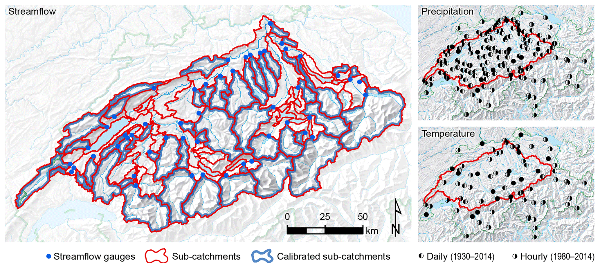
Figure 1Overview map of the Aare River basin, showing data series available for streamflow (left panel), precipitation (top-right panel) and temperature (bottom-right panel). The streamflow map also reveals the 80 sub-catchments used in hydrological modelling and which of these were calibrated. Map background: Federal Office of Topography swisstopo.
The main sources of data were meteorological and hydrological records from stations operated by the Swiss Confederation (Federal Office for the Environment, 2016; MeteoSwiss, 2016) and by cantonal agencies. The meteorological data encompass continuous records of daily precipitation (1930–2014) at 105 sites (of which 78 are located within the Aare River basin), daily temperature (1930–2014) at 26 sites (17 within the Aare River basin), hourly precipitation (1990–2014) at 65 sites (24 within the Aare River basin) and hourly temperature (1990–2014) at 67 sites (25 within the Aare River basin) (Table S1 in the Supplement). In addition, an extended dataset of daily precipitation records (1864–2014) at 666 sites was available, although it contains many missing values. For the period with only daily continuous records (1930–1989), hourly precipitation and temperature values were obtained by disaggregation. This disaggregation used the temporal structure of the respective variable observed, either for the same day if available at a nearby station or for an analogous day in the period with hourly continuous observations. The analogy was specified using surface weather for the region and applying constraints to preserve season and class of intensity following Breinl and Di Baldassarre (2019). The hydrological data encompass continuous discharge records at 65 stations (Table S2). The hourly hydrological data (1974–2014) have a median length of 36 years, with a range of 15–41 years; the daily hydrological data (1930–2014) also have a median length of 36 years but with a range of 16–85 years. In addition, records of annual maximum floods were available for some of these stations. These records date back even further, with a median length of 94 years and a range of 32–111 years. For the 44 streamflow measurement stations operated by the Federal Office for the Environment (FOEN), two different extrapolations of the observed annual maximum floods were available: the FOEN approach (Baumgartner et al., 2013), which extrapolates at-site measurements via the generalized extreme value (GEV) distribution, and the EPFL approach (École polytechnique fédérale de Lausanne; Asadi et al., 2018), which combines at-site measurements with measurements from a group of similar catchments for fitting the parameters of the GEV distribution.
Several detailed hydraulic simulations with BASEMENT (Vetsch et al., 2018) were available from the EXAR project, covering relevant sites along the main branches of the Aare River system (Pfäffli et al., 2020). These simulations represent the behaviour of the river system at flows with return periods of 100, 1000 and 10 000 years, particularly as regards bank overflow and floodplain retention (Staudinger and Viviroli, 2020), and were used to parameterize the hydrological routing (Sect. 3.3.2).
Regulation rules for the large lakes (Lake Biel, surface area of 39.8 km2; Lake Brienz, 29.8 km2; Lake Lucerne, 113.6 km2; Lake Thun, 48.4 km2; Lake Zug, 113.6 km2; Lake Zurich, 90.1 km2) were provided by the corresponding authorities. Depending on the lake, the rules are aimed at diverse and partly contradicting targets such as protecting settlements downstream from floods, avoiding inundation of the lakeside areas, preserving habitats, keeping natural stage fluctuations and ensuring lake navigation. The information available ranged from detailed stage–discharge diagrams at a daily or monthly scale to rough indications of target discharge values for different intervals of lake level. For the two remaining small regulated lakes (Lake Ägeri, 7.2 km2; Lake Lauerz, 3.1 km2), the impact of regulation on flows at the critical sites was considered minor and thus neglected; this is also because in both of these cases, another regulated lake with considerably larger surface area is located downstream.
Finally, reconstructions of selected historical floods were also available. Departing from a comprehensive pilot study by Wetter (2015), four historical events were analysed in more detail within the EXAR project (Baer and Schwab, 2020). The focus was on events that could be reconstructed for more than one site, cover different seasons and represent different states of the river corrections in Switzerland (Table 1).
Table 1Reconstructed historical (1480, 1570, 1852, 1876) and observed recent (2005, 2007) peak discharges for three sites along the Aare River (see Wetter, 2015; Baer and Schwab, 2020), as well as the most extensive changes made to the river network (1714, 1878) (see Vischer, 2003).
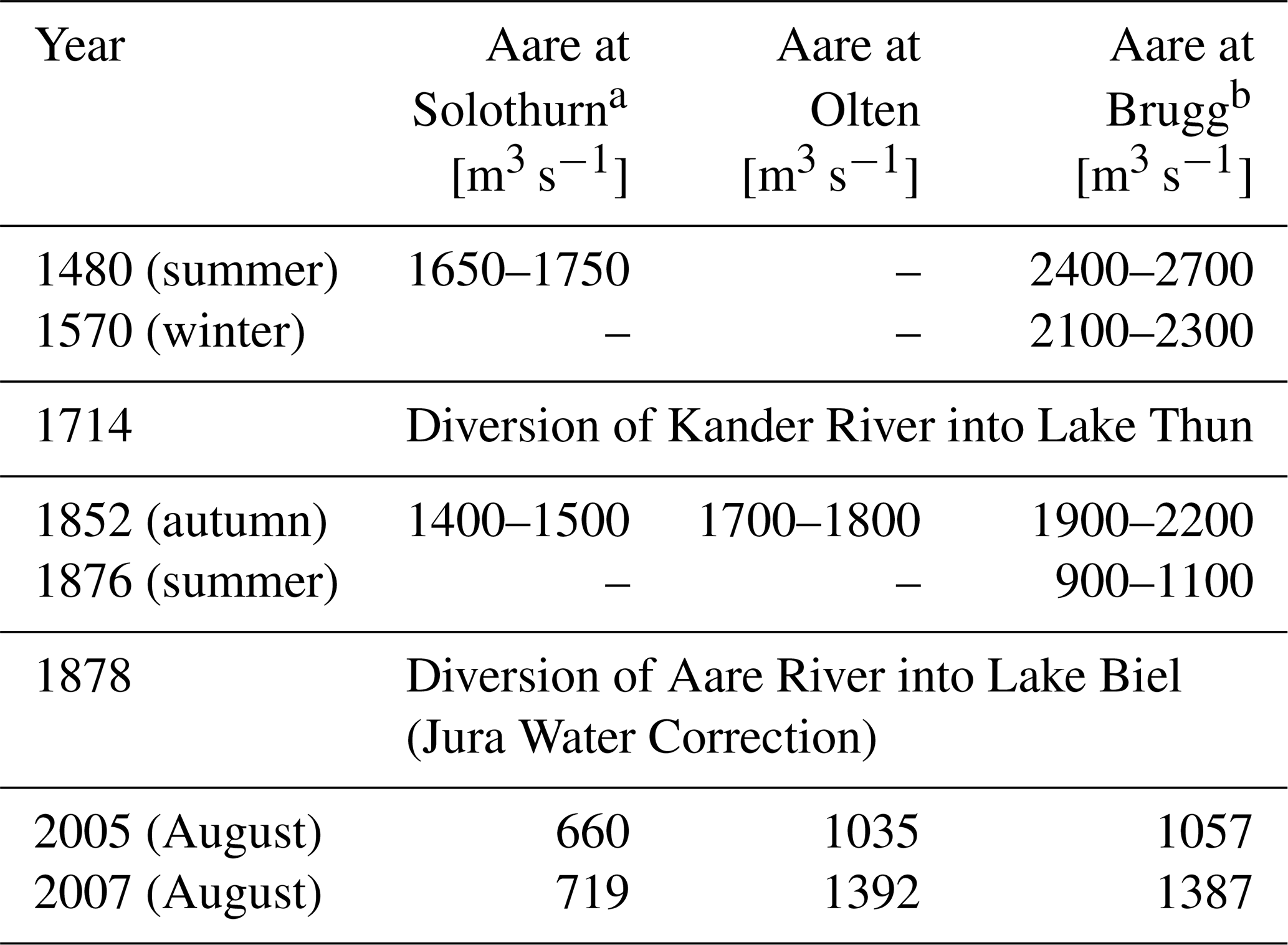
a Values for 2005 and 2007 are observations for Aare at Brügg–Aegerten that were routed downstream to Solothurn with BASEMENT (see Baer and Schwab, 2020; Pfäffli et al., 2020). b Values for 2005 and 2007 are observations from sites Aare at Murgenthal, Wigger at Zofingen and Dünnern at Olten that were routed downstream to Aare at Olten with BASEMENT (see Baer and Schwab, 2020; Pfäffli et al., 2020).
3.1 Study set-up
Our model chain consists of three main components. First, two weather generators – GWEX (Generator of Weather EXtremes; Sect. 3.2.1) and SCAMP (Sequential Construction of atmospheric Analogs for Multivariate Weather Predictions; Sect. 3.2.2) – were used to provide 30 time series scenarios of precipitation and temperature with a length of 10 000 years each and to assess the structural uncertainty in the meteorological part of this study (Sect. 5.3 and 5.5). Second, the full outputs of GWEX were used as input for the bucket-type catchment model HBV (Hydrologiska Byråns Vattenbalansavdelning; Sect. 3.3.1), run at an hourly time step for 80 sub-catchments that cover the entire Aare River basin. From SCAMP, selected scenario years that contain large precipitation events were also run through the HBV model (Sect. 5.3). Third, simulation results from the individual sub-catchments were routed downstream using the routing system RS MINERVE (Sect. 3.3.2) for a representation of the entire Aare River system. The final simulation outputs span roughly 300 000 years at an hourly time step and cover 19 critical sites (including the Aare River outlet; see Sect. 3.3.2) as well as the outlets of the 80 sub-catchments simulated with HBV (Fig. 2, Tables S2 and S3).

Figure 2Overview map of the Aare River basin, showing model outputs of HBV light (orange) and RS MINERVE (red) as well as the two major sub-basins (Reuss and Limmat rivers) (green). Results from RS MINERVE are discussed further below for the Aare River at Halen (1), Golaten (2), Brügg–Aegerten (similar to the Lake Biel outlet) (3), Aarburg (4) and Brugg (5); the Reuss River outlet (6); the Limmat River outlet (7); and the Aare River at Stilli (close to its outlet) (8). Map background: Federal Office of Topography swisstopo.
The choice of models was motivated by the specific requirements of CS, namely to cover a wide range of possible meteorological and hydrological conditions rather than the high spectrum of precipitation and streamflow only. In addition, the model chain had to be suitable for mountainous environments (i.e. consider rain–snow partitioning of precipitation and representing snowpack as well as glaciers) and allow for a considerable number of hydrological and hydraulic complexities (i.e. lake retention and regulation, reservoir management, bank overflow, floodplain retention) to be represented. Finally yet importantly, each of the individual models had to be computationally efficient due to the vast extent of hourly simulations for a large number of sub-catchments. This requirement precluded the use of models with more detailed physical-process formulations. Since all models used here have been described and tested individually, we provide only a short introduction below and refer to published literature for more details, including validation. It would certainly have been possible to use different models of similar complexity in each of the three model chain links. However, the scope of the present study was to explore the feasibility of the CS approach for multiple sites in a large river basin at high temporal resolution, using models that have demonstrated suitability for the spatial domain and goals in focus.
3.2 Weather generator
3.2.1 GWEX
GWEX is a multi-site, two-part stochastic weather generator for precipitation and temperature that relies strongly on the structure proposed by Wilks (1998). GWEX aims to reproduce the statistical behaviour of weather events at different temporal and spatial resolutions, with a focus on extremes. Since comparatively long events are relevant in the Aare River basin, GWEX generates 3 d precipitation amounts in a first step. These amounts are then disaggregated to daily and ultimately hourly values using meteorological analogues.
The precipitation occurrence process of GWEX is represented for each site by a two-state first-order Markov chain that generates 3 d sequences with or without precipitation. The seasonality of this occurrence process is considered by estimating model parameters independently for each month of the year. Inter-site correlations between precipitation occurrence are introduced using a multivariate Gaussian distribution. For 3 d sequences with precipitation, the extended GP-Type III distribution (E-GPD; generalized Pareto distribution) (Papastathopoulos and Tawn, 2013) is then used to generate 3 d precipitation amounts at each site. This distribution can be described by a smooth transition between a gamma-like distribution and a heavy-tail generalized Pareto distribution (GPD) and has been shown to model precipitation intensities adequately (Naveau et al., 2016).
The shape parameter of the distribution is estimated with a robust regional advanced method (Evin et al., 2016) using the extended dataset of 666 stations. Spatial and temporal dependence of 3 d precipitation amounts is represented using a first-order multivariate autoregressive model. A Student copula represents the dependence structure of innovations in the multivariate autoregressive model (MAR) and introduces a tail dependence between at-site extremes. Similar to the occurrence process, the seasonality of the precipitation intensity is taken into account by fitting the model for each month using a 3-month moving window.
For temperature, GWEX uses the skew exponential power (SEP) distribution (Fernandez and Steel, 1998) to model the standardized daily temperature at each station and a MAR model to represent the spatial and temporal dependence structures simultaneously. The seasonal cycles are accounted for with non-parametric functions, and the generation is additionally conditioned on precipitation of the current generation day.
Further details on GWEX can be found in Evin et al. (2018, 2019).
3.2.2 SCAMP
SCAMP is a hybrid weather generator based on atmospheric and weather analogues and is methodologically fully independent of GWEX (Raynaud et al., 2017, 2020; Chardon et al., 2018). It generates long series of synoptic weather over Europe in a first step, using the ERA20C atmospheric reanalysis 1900–2010 (Poli et al., 2016) as point of departure. New atmospheric trajectories are possible by rearranging the atmospheric sequences observed within the 110 years covered by ERA20C. A detailed description of the simulation process is given in Chardon et al. (2016) and Raynaud et al. (2020). The resulting long series of synoptic weather are then used to generate daily weather for the Aare River basin. To this end, a stochastic downscaling model based on atmospheric analogues is applied (Chardon et al., 2016; Raynaud et al., 2020). For each day within the long time series of synoptic weather, the K-nearest atmospheric analogue days are identified in the archive period 1930–2010 where both ERA20C data and station records are available. The regional weather scenario for the day in question is then generated from the statistical distribution of the regional weather observed for those K analogues. As shown by Mezghani and Hingray (2009) and Chardon et al. (2014), the accuracy of statistically downscaled weather scenarios typically increases with spatial aggregation. In the present work, the K-nearest analogue days are thus used to generate the regional weather, namely mean areal precipitation (MAP) and mean areal temperature (MAT) for the Aare River basin. For the current generation day, the regional weather scenario is generated from the statistical distribution of the regional weather observed for those K-nearest analogue days (Chardon et al., 2018). The criterion used to identify the nearest analogues is a measure of the similarity of (1) the dynamic of atmospheric circulation at a synoptic scale and (2) the thermodynamic state of the atmosphere at a regional scale. For this, we consider in a two-step identification process (1) the spatial shape of fields of geopotential heights at 1000 and 500 hPa and (2) the mean regional-scale vertical velocity at 600 hPa and the September–May temperature at 2 m. In summer, large-scale precipitation is used instead of vertical velocity, since it has better predictive power for convective phenomena at the coarse resolution of the reanalysis data.
3.2.3 Temporal disaggregation
For the hydrological simulations at the sub-catchment scale, sub-daily data were needed. For both GWEX and SCAMP, this disaggregation was based on weather analogues: for each day in the simulation period, the daily weather variables obtained with the weather generator were disaggregated according to the spatial and temporal structure of an analogous day for which hourly observations were available in the period 1990–2014. The analogue day candidates were identified using a distance criterion (the root mean square error, RMSE) which measures the similarity between the regional weather situation of the target generated day and that of the observations. For GWEX, the regional weather situation of a given day was described by the spatial field of the weather variable considered, namely the daily value of the variable available at the multiple gauge stations in the area. For SCAMP, the regional weather situation was described with the regional MAP and MAT scenarios generated in the first step of the generation process. This disaggregation approach directly exploits past observed spatiotemporal structures and imposes the relative distribution of the candidate day (i.e. the sub-daily distribution of the precipitation and temperature values, as well as the sub-regional distribution, so-called fragments) on the day of interest. This approach, also called the “method of fragments” (Buishand and Brandsma, 2001), is described in detail in Appendix 10.2 of Staudinger and Viviroli (2020) for GWEX scenarios and in Mezghani and Hingray (2009) for the simulation context of SCAMP.
3.2.4 Mean areal values
As the HBV model requires mean areal values of precipitation and temperature as inputs for a given sub-catchment (i.e. MAP and MAT), we have processed the outputs of the two weather generators as follows: for GWEX, the simulated MAP and MAT values for each sub-catchment were obtained using the Thiessen (1911) polygon method applied to the weather scenarios produced at the multiple sites. For SCAMP, simulated MAP and MAT were directly obtained from the spatiotemporal disaggregation of MAP and MAT values generated at the regional scale (see Sect. 3.2.3).
3.3 Hydrological model and routing
3.3.1 HBV model
For the hydrological catchment runoff simulations, the HBV model (Bergström, 1972, 1992; Seibert and Bergström, 2022) was used in the version HBV light (Seibert, 1997; Seibert and Vis, 2012). The choice of HBV was motivated by its fast processing speed (necessary for running long CS for many sub-catchments) and its well-documented suitability for flood estimation in Switzerland (Horton et al., 2022). HBV is a semi-distributed bucket-type model that uses time series of mean areal precipitation and mean air temperature as inputs. These inputs were distributed within the catchment along predefined elevation zones (here with an extent of 100 m) using a constant lapse rate for temperature (decrease of 0.6 ∘C for 100 m increase in elevation) and a constant adjustment factor for precipitation (linear increase of 5 % for 100 m increase in elevation; see e.g. Farinotti et al., 2012; Ménégoz et al., 2020; Ruelland, 2020). Actual evapotranspiration was estimated from the long-term daily mean of potential evaporation according to Primault (1962, 1981) in combination with observed temperature and simulated soil moisture.
The standard version of HBV consists of four main routines that represent snow processes, soil moisture, groundwater and streamflow routing in the channel. These modules entail 15 tunable parameters. For sub-catchments with a glacier cover of 5 % or more, an additional glacier routine with five tunable parameters was activated (Seibert et al., 2018). A total of 50 gauged sub-catchments (median catchment area: 117 km2; see Fig. 1) were calibrated, focusing on sites without major impacts from hydropower, lake regulation, bank overflow and floodplain retention. For calibration a genetic algorithm (Seibert, 2000) was used with a multi-objective function that consists of Nash–Sutcliffe efficiency (Nash and Sutcliffe, 1970; weight of 0.3), peak efficiency (Seibert, 2003; weight of 0.5) and mean absolute relative error (weight of 0.2). To account for parameter uncertainty, 100 independent model calibrations were performed for each sub-catchment, and the corresponding parameter sets were retained. From this pool of 100 parameter sets, 3 representative sets were subsequently selected using a clustering approach to cover low, intermediate and high response in simulated peak flows as proposed by Sikorska-Senoner et al. (2020). For the remaining 30 ungauged sub-catchments, parameters were estimated from the calibrated sub-catchments using a clustering algorithm that takes the discharge regime as a discriminant and then selects two donor sub-catchments (Kauzlaric et al., 2021). From each of these two donors, the best-performing 50 parameter sets were transferred to obtain again a total of 100 parameter sets for each sub-catchment. From these 100 sets, 3 representative sets were selected subsequently, as done for calibrated sub-catchments. For details on calibration, parameter set selection and regionalization we refer to Kauzlaric et al. (2020, 2021).
3.3.2 RS MINERVE
Discharge of the individual sub-catchments simulated with HBV light was finally combined and routed using the hydrological routing system RS MINERVE (García Hernández et al., 2020). As with HBV, the main reasons for using RS MINERVE were its speed and well-documented applications in Switzerland (Horton et al., 2022). The simplified representation of the Aare River system built in RS MINERVE emulates more detailed 2D hydraulic simulations of synthetic hydrographs with BASEMENT (see Sect. 2). To cover a broad spectrum of possible event magnitudes and explore the effect of lake regulations, synthetic hydrographs with return periods of 100, 1000 and 10 000 years were considered. Major effects of bank overflow and floodplain retention – resulting in attenuation and retardation of the flood peak – were considered across a wide range of discharges by implementing channels both in series and in parallel at relevant sites. These channels account for estimated channel flow capacity and inundated areas. Levee breaks, by contrast, have not been implemented. For all of the nine major lakes (Biel, Brienz, Gruyère, Lucerne, Murten, Neuchâtel, Thun, Zug and Zurich), stage–area–volume relationships were extracted from digital terrain information (swisstopo, 2005). Six of these lakes (Biel, Brienz, Lucerne, Thun, Zug and Zurich) are regulated, and the regulation rules are usually expressed as stage–discharge relationships with seasonal, monthly or even daily variation. These rules were digitized and implemented into RS MINERVE, where necessary in a slightly simplified form. Where available and feasible, rules applied in the case of flood events (i.e. deviating from business-as-usual operation) were implemented. For example, discharge in the Aare River is limited to 450 m3 s−1 downstream of Lake Thun in Bern and to 850 m3 s−1 downstream of Lake Biel in Murgenthal for as long as possible. If the level of a lake rises above the flood stage (i.e. the level above which widespread inundations occur; see flood danger levels defined by Federal Office for the Environment, 2022), stage–discharge relationships as simulated in BASEMENT assuming open weirs are used. The output nodes themselves were set at locations where river valley morphology prevents extensive floodplain inundation, and thus all discharge flows through the main river channel. This procedure was motivated by the need to partition 2D hydraulic modelling in EXAR into independent subsystems (Pfäffli et al., 2020).
Due to the exceptionally high computational cost of long simulations at multiple sites, it was only possible to run the full set of GWEX-generated weather scenarios through HBV light and RS MINERVE. From the 300 000 years simulated in total, 11 000 were discarded due to an inconsistency (most likely caused by a file transfer problem and the subsequent usage of an outdated version of GWEX data; for details, see Viviroli and Whealton, 2020), leaving 289 000 years for detailed analysis.
From SCAMP, only a selection of scenario years containing the highest cumulative precipitation events were considered and run through the hydrological model and routing due to computational time limitations. For each of five accumulation periods (1, 3, 7, 30 and 60 d) and six perimeters (the entire Aare River basin as well five large sub-regions), the years containing the 300 largest events were identified, leading to a total of 3425 individual years after the elimination of duplicates. To avoid assumptions about initial conditions, a warm-up period of 10 years was implemented using the SCAMP scenario data preceding the respective event.
Note that the present implementation is not expected to be suitable for catchments with an area of less than roughly 1000 km2, both due to the initial 3 d cycle of GWEX and the hourly temporal resolution of the simulations. These specifics are unsuitable for smaller catchments where convective events become more decisive for flood behaviour (Sikorska et al., 2015).
In the following presentation of results, we start by investigating the performance of each model in the model chain individually. We then proceed to results as simulated by the entire model chain, looking both at sub-catchments as well as critical sites in the Aare River system. Although results of the entire chain are decisive for assessing the reliability of the CS approach in the present context, scrutiny of the individual chain links ensures that all components of the chain produce reasonable outputs and work well for the right reasons (Klemeš, 1986; Kirchner, 2006). We finally provide an overview of the spatial patterns in the most prominent events simulated for the entire Aare River basin.
4.1 Weather generator
This subsection presents an evaluation of the performances of GWEX and SCAMP at the daily scale, by comparison to observations covering the period 1930–2014. Similar evaluations at the hourly scale are not provided because the shorter period 1990–2014 covered by the hourly observations limits the evaluation of extreme values for large return periods.
4.1.1 GWEX
As shown by Evin et al. (2018, 2019), GWEX can reproduce the major characteristics of precipitation and temperature observations at all spatial and temporal scales considered here. Figure 3a shows the empirical return levels of maximum 1 d mean areal precipitation (MAP1d) obtained from the 30 time series of 10 000 years each for the entire Aare River basin as well as for five main sub-regions (see Fig. 10). Figure 4a shows the same for 3 d mean areal precipitation (MAP3d). For short return periods, for which return levels can also be estimated from observed mean areal precipitation, the return levels of the simulations are very close to the empirical ones and highlight the good performance of the model for those variables. For the entire Aare River basin as well as for the Neuchâtel, Thun and Aare–Emme sub-regions, most of the 18 000-year return levels were between 130 and 160 mm for MAP1d and between 190 and 225 mm for MAP3d. For the two easternmost sub-regions (Reuss and Limmat), the values were slightly higher, between 160 and 205 mm for MAP1d and between 230 and 270 mm for MAP3d.
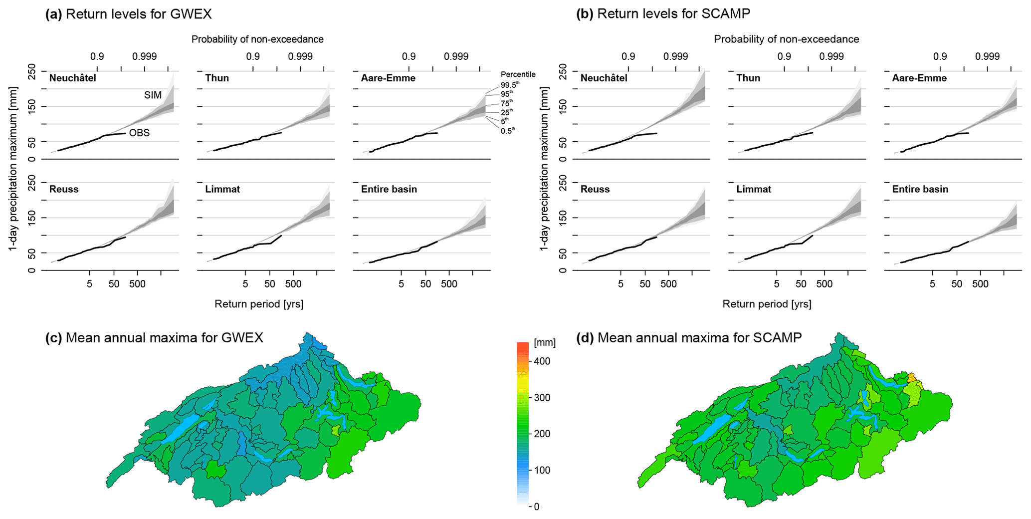
Figure 3(a, b) Empirical return levels obtained for MAP1d (1 d mean areal precipitation) from the 30 time series of 10 000 years generated with GWEX (a) and SCAMP (b) for the entire Aare River basin and five main sub-regions using the Gringorten plotting position. The bounds of the grey-shaded areas correspond to the 0.5th/99.5th, 5th/95th and 25th/75th percentiles of the 30 time series, respectively. (c, d) Mean maximum simulated MAP1d from the 30×10 000-year time series for each of the 80 HBV sub-catchments (c: GWEX, d: SCAMP); major lakes are drawn in cyan. Note that the largest simulated MAP value in one 10 000-year-long simulation corresponds to a return period of 18 000 years (Gringorten plotting position). Also note that the extreme MAP values mapped do not necessarily occur simultaneously, i.e. do not correspond to one single event.
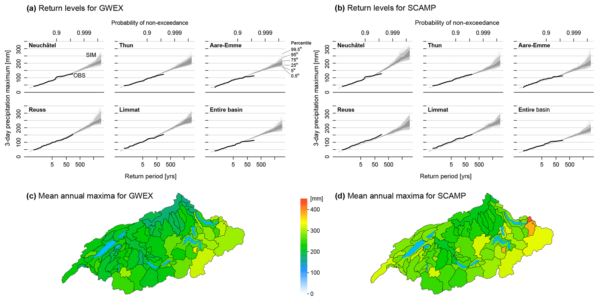
Figure 4(a, b) Empirical return levels obtained for MAP3d (3 d mean areal precipitation) from the 30 time series of 10 000 years generated with GWEX (a) and SCAMP (b) for the entire Aare River basin and five main sub-regions using the Gringorten plotting position. The bounds of the grey-shaded areas correspond to the 0.5th/99.5th, 5th/95th and 25th/75th percentiles of the 30 time series, respectively. (c, d) Mean maximum simulated MAP3d from the 30×10 000-year time series for each of the 80 HBV sub-catchments (c: GWEX, d: SCAMP); major lakes are drawn in cyan. Note that the largest simulated MAP value in one 10 000-year-long simulation corresponds to a return period of 18 000 years (Gringorten plotting position). Also note that the extreme MAP values mapped do not necessarily occur simultaneously, i.e. do not correspond to one single event.
Similar patterns are visible in the mean largest GWEX values for MAP1d (Fig. 3c) and MAP3d (Fig. 4c) in the sub-catchments, i.e. the average of the largest events in each of the 30 different time series. The largest values were again found in the southeast of the Aare River basin (200–280 mm for MAP1d, 280–350 mm for MAP3d). Large values were also obtained in the Jogne River sub-catchment in the Canton of Fribourg (220 mm for MAP1d, 297 mm for MAP3d). In the west, close to the Jura Mountains, the values were slightly smaller (160–200 mm for MAP1d, 210–270 mm for MAP3d). Similar results were obtained for the central part of the Aare River basin. The lowest values were found in the north (120–150 mm for MAP1d, 160–210 mm for MAP3d).
The performance of GWEX with regard to additional characteristics was also evaluated. For instance, Fig. 5 highlights the very good performance of GWEX for the estimation of 1 and 3 d precipitation distribution at six selected representative stations, as well as for the reproduction of wet and dry spells and for the monthly precipitation amounts at different spatial scales (the entire Aare River basin, large sub-regions and the six representative stations). For a detailed evaluation of the model, we refer to Evin et al. (2018, 2019).
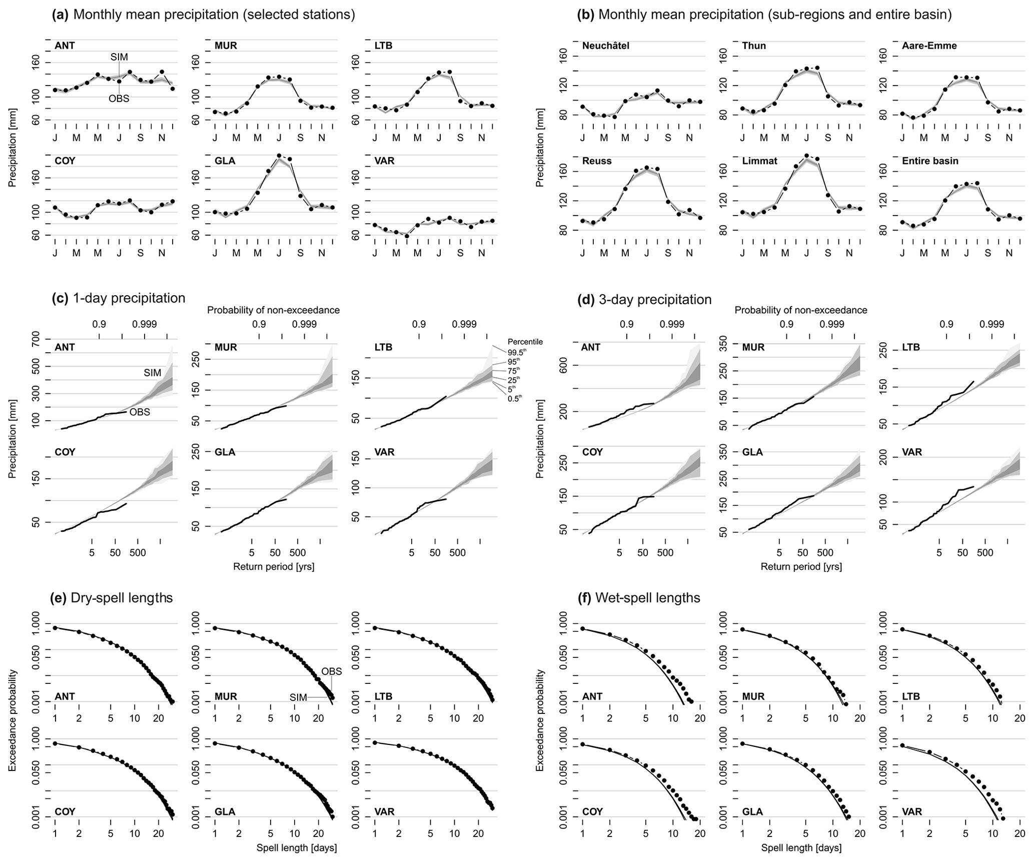
Figure 5Multiscale evaluation of GWEX regarding monthly mean precipitation (a, b), 1 and 3 d precipitation (c, d), dry-spell lengths (e), and wet-spell lengths (f). Results for panels (a) and (c)–(f) are for six selected representative stations, namely Andermatt (ANT), Muri (MUR), Lauterbrunnen (LTB), Courtelary (COY), Glarus (GLA) and Valeyres-sous-Rances (VAR) (see Table S1); results for panel (b) are for five main sub-regions (see Fig. 10) and the entire Aare River basin. Observations are drawn in black; GWEX results are in grey.
4.1.2 SCAMP
Similar to GWEX, SCAMP can reproduce the characteristics of precipitation and temperature observations at all spatial and temporal scales considered here (see Raynaud et al., 2020, for an evaluation of SCAMP at the catchment scale and Chardon et al., 2020, for an evaluation at different spatial scales). Whatever the timescale under consideration, the 30×10 000-year-long weather time series also present meteorological situations that cannot be found in the observations (Raynaud et al., 2020). For all four seasons, the ranges of simulated seasonal temperature and precipitation exceed the observed ones. For instance, the minimum and maximum observed winter precipitation amounts are 60 and 490 mm, respectively. In the SCAMP simulations, these values reached 40 and 690 mm. Such characteristics are particularly interesting for hydrological purposes, as they allow for simulating extreme discharge events with unobserved initial conditions in terms of soil moisture and snowpack.
Results for precipitation maxima are presented on the right-hand sides of Fig. 3 (MAP1d) and Fig. 4 (MAP3d), for similar spatial and temporal scales as for GWEX. Good agreement is obtained between observations and simulations for return periods of up to 150 years, which corresponds to the maximum return period that can be estimated with the Gringorten (1963) formula on the basis of 85 years of observed data. For the entire Aare River basin, the 18 000-year MAP1d was 140 mm on average but reached almost 200 mm for some scenarios. For MAP3d, these values reached 190 and 250 mm, respectively, showing that for high-precipitation events, 75 % of the total amount fell within 24 h. For both MAP1d and MAP3d, the Limmat and the Neuchâtel sub-regions received slightly larger precipitation events, with an additional 20–40 mm compared to the other sub-regions. This is even more visible from the return level maps associated with the maximum return periods for the 80 sub-catchments. Similar to the results of GWEX, the higher precipitation values are located in the far southeast of the Aare River basin and the western part of the area, close to the Jura Mountains. Noticeable are the large differences from one sub-catchment to the other, with amounts ranging from 150–350 mm for MAP1d and 200–450 mm for MAP3d. This uneven spatial structure is also visible in the observations for the 150-year return period.
At the scale of the entire Aare River basin, MAP extremes are roughly similar for GWEX and SCAMP (Figs. 3 and 4). At the sub-catchment scale, however, the extremes of SCAMP are generally larger than those of GWEX and show slightly different spatial patterns. Both of these differences are probably explained by the fact that the two weather generators are built upon substantially different approaches and generation processes: GWEX produces multi-site 3 d amounts disaggregated to a daily scale, whereas SCAMP produces regional MAP and MAT values at a daily scale. The 3 d maxima in SCAMP are thus the result of the aggregation of three consecutive daily simulated values. The temporal coherency between MAP values generated by SCAMP for consecutive days comes from the large-scale atmospheric forcing, which follows relevant atmospheric trajectories from a single day to the next. However, this conditioning does not necessarily preserve the day-to-day dynamics of rainfall systems. Nevertheless, it can be noticed that the largest difference – found for the Neuchâtel sub-region – is rather moderate (+10 % for MAP3d and +20 % for MAP1d). A further comprehensive evaluation of precipitation time series generated with both weather generators is found in Evin et al. (2018, 2019) and Chardon et al. (2020), as well as in Raynaud et al. (2020), which reports on severity, spatial and temporal dynamics, and meteorological relevance of events.
4.2 Hydrological model
Hydrological simulations for the individual HBV sub-catchments were evaluated based on three criteria: the Nash–Sutcliffe (NSE) (Nash and Sutcliffe, 1970), the Kling–Gupta (KGE) (Gupta et al., 2009) and the non-parametric Kling–Gupta (KGE_NP) (Pool et al., 2018) efficiencies. These criteria indicated at least acceptable results in most cases (Fig. 6a) with reference to hourly discharges in the period 1974–2014 (effective length of records per station, see Table S2), meaning that the overall streamflow behaviour was simulated reasonably well. The sub-catchments with poor results have a widespread occurrence of karstic rock or are affected by regulated lakes. Both of these influences are not depicted explicitly in the HBV model. The three representative parameter sets achieved rather similar median efficiencies, with the upper representative parameter set showing a tendency towards a larger spread.
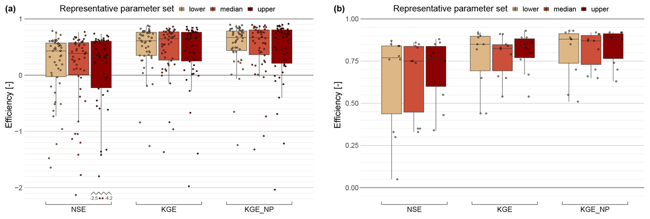
Figure 6Model efficiencies at an hourly time step over the period 1974–2014 for HBV (a: 50 gauged sub-catchments) and RS MINERVE (b: 10 gauged output nodes) showing the three representative parameter sets. The efficiency criteria used are Nash–Sutcliffe (NSE), Kling–Gupta (KGE) and non-parametric Kling–Gupta (KGE_NP). All criteria have an upper bound of 1 (which means ideal performance) and are unbounded towards the bottom.
An evaluation for the largest observed flood events regarding peak and volume (May 1986, June 1987, July 1987, August 1987, May 1994, May 1995, May 1999, August 2005, August 2007) showed absolute differences mainly in a range as narrow as ±1 mm h−1. Within this range, the larger sub-catchments showed more minor deviations than the smaller sub-catchments, meaning differences are smaller in the sub-catchments that contribute high discharge to the overall Aare River basin. The largest deviation was found for the Steinenbach River catchment (range of −3 to +2 mm), which is the smallest sub-catchment considered in the study (surface area: 19.1 km 2). The higher reliability of results for large catchments could be due to more precipitation stations being available for interpolation in space (Girons Lopez et al., 2015). Results did not show systematic patterns of some events being simulated less accurately than others. In addition, none of the three representative parameter sets showed clearly worse or better performance than any other.
4.3 Hydraulic routing
4.3.1 Individual evaluation
The hydrological routing was first validated individually for the output nodes of RS MINERVE in the Aare River system. For this, synthetic events with an estimated return period of 10 000 years were fed directly into the relevant river stretches in RS MINERVE. The peak flow values of these events were determined on the basis of the regional statistical model by Asadi et al. (2018). Results were then compared with detailed hydraulic simulations in BASEMENT using the same synthetic events as input. Such individual comparisons without use of the HBV outputs were also performed for large observed events of the last few decades. These comparisons showed that RS MINERVE is able to reproduce the discharge behaviour of both large observed as well as even larger synthetic events (Kauzlaric et al., 2020).
4.3.2 Joint evaluation with hydrological simulations
The efficiency of the routing was then evaluated in more detail in combination with hydrological simulations for the observed period 1974–2014. The criteria and period of this joint RS MINERVE–HBV evaluation were similar to those used for evaluating the hydrological simulations individually (see Sect. 4.2). The evaluation was possible for 10 sites where streamflow records were available at reasonably close distance to RS MINERVE output nodes (see Table S3). The outlets of lakes were not evaluated because lake retention and regulation strongly attenuate flow dynamics, and efficiency assessments are therefore of limited value only. Results (Fig. 6b) show good to very good agreement between observations and simulations (median efficiencies over all three representative parameter sets: NSE 0.83, KGE 0.85, KGE_NP 0.89) for all sites in the Aare, Reuss and Limmat rivers. The three sites in the Emme, Lorze and Saane rivers showed poorer performance (NSE 0.34, KGE 0.65, KGE_NP 0.66). A similar joint RS MINERVE–HBV evaluation was done for an extended period 1930–2014 using disaggregated meteorological data as input to HBV. While the corresponding simulations were done at hourly resolution, evaluation was only possible at a daily time step because streamflow observations before 1974 were available in digital form at a daily resolution only. Efficiency criteria for this longer period (not shown) were similar or even slightly higher than for the period 1974–2014 (Kauzlaric et al., 2020).
4.4 Entire simulation chain
4.4.1 Discharge characteristics
When running the full hydrometeorological model chain with weather generator scenarios instead of observed weather, there are obviously no reference observations available for evaluating streamflow results. The focus was therefore put on two selected aspects of streamflow and flood behaviour, namely the cumulative frequency of streamflow and seasonality of annual maximum floods (AMFs). The following evaluations are based on the full 289 000 years of CS using GWEX inputs. Selected results on the basis of SCAMP inputs are only discussed in Sect. 5.3, since it was necessary to limit simulations to a sample of 3425 years containing the largest cumulative precipitation events (see Sects. 3.1 and 3.3.2).
To assess cumulative frequency of streamflow, flow duration curves (FDCs) of simulated hourly streamflow based on GWEX were computed for all 50 gauged HBV sub-catchments as well as for the 10 RS MINERVE outputs for the total Aare River system close to measurement sites. For comparison, FDCs were derived from the observations that comprise roughly 30–40 years of data, depending on the gauging station. In this comparison, the HBV simulations based on GWEX were very similar to the observations for most sub-catchments (Fig. S1 in the Supplement). Larger differences were found for two sub-catchments only: Simme at Latterbach, where uncertainties in the discharge measurements might explain the discrepancy, and Chise at Freimettigen, where karst may be responsible. The differences between the three representative parameter sets were minimal. The RS MINERVE outputs for the total Aare River system proved mostly very similar as well (Fig. S2a). Larger differences were found for the Lorze River outlet (area: 289 km2), with systematically higher simulated values for more frequent flows and lower simulated values for high flows. Also at this site, the differences between the three representative parameter sets were the largest, while they were generally small for all other sites examined. Plotting FDCs of the highest 10 % of simulated flows (Fig. S2b) revealed a general tendency to higher simulated discharge for Aare at Brügg–Aegerten and again further downstream for Aare at Brugg, stemming from rather high simulated discharges of large tributaries (Saane and Emme rivers, respectively).
To assess flood peak characteristics, we computed the seasonality of AMFs using GWEX scenarios as an input and compared this against similar simulations using disaggregated observations as an input (see Staudinger and Viviroli, 2020). The seasonality was evaluated via the Julian date on which the annual maximum flood (AMF) occurs, and the variability in the AMF occurrences was quantified with a dimensionless measure of the spread of the data (Burn, 1997). The analyses were first done for each HBV sub-catchment independently, meaning that in each sub-catchment a different event may have been classified as the AMF. As the difference between the three representative parameter sets mainly affected the magnitude of the AMFs but not their seasonality or the time of the occurrence, the seasonality was analysed for the median representative parameter set only. For comparison, we computed the seasonality of the simulations with disaggregated weather observations (1930–2014). Comparison (Fig. S3a) shows similar results for most of the sub-catchments. The differences that appear in some sub-catchments should not be overemphasized, since the sample size of the GWEX-based run (AMFs from 289 000 years of simulation) was much larger than that of the run based on disaggregated observations (AMFs from 85 years of simulation), meaning that the latter contains a comparatively small subset of possible events and corresponding seasons. Overall, however, the larger picture of seasonality has a comparable pattern. The seasonality patterns for sites in the Aare River system (Fig. S3b) are strongly affected by the regulated pre-alpine lakes, and overall, a slightly earlier mean date of AMF occurrence was noted in the GWEX-based simulations with RS MINERVE, except for the outlet of Lake Lucerne (VieSee). On average, AMFs occurred 12 d earlier in GWEX-based simulations; the maximum difference was 33 d earlier. Here, it is again important to note that the sample size is different, and a slight disagreement should not be overemphasized.
4.4.2 Flood exceedance curves
The exceedance curves of AMFs derived from the full CS of 289 000 years are shown in Fig. 7 for six selected sites in the Aare River basin. For the Aare River at Halen, CS results based on GWEX are higher than observations for return periods of roughly 10 to 100 years but otherwise agree well. Downstream at Golaten, CS is generally higher than observations, FOEN extrapolations (Baumgartner et al., 2013) and EPFL extrapolations (Asadi et al., 2018), while EPFL extrapolations are clearly lower than CS, observations and FOEN extrapolations for return periods larger than 100 years. The outflow of Lake Biel then shows the strong retention effect of the Jura lake system, leading to a marked reduction in the largest peak discharges. This effect is visible in both observation- and simulation-based data, whereas CS is midway between the two observation-based estimates of FOEN and EPFL. Due to the further inflows downstream of Lake Biel, peak discharges increase notably again, and CS results agree very well here with the values expected from statistical extrapolation of observed events. Discrepancies occur mainly for return periods of more than 100 to 1000 years, where CS shows higher values. The simulations using disaggregated observations of temperature and precipitation for 1930–2014 show high agreement with observations as well. This is also the case for Aare at Golaten, where CS achieved higher AMFs in comparison to observations and extrapolations. A discussion of differences with explanations will follow in Sect. 5.2.
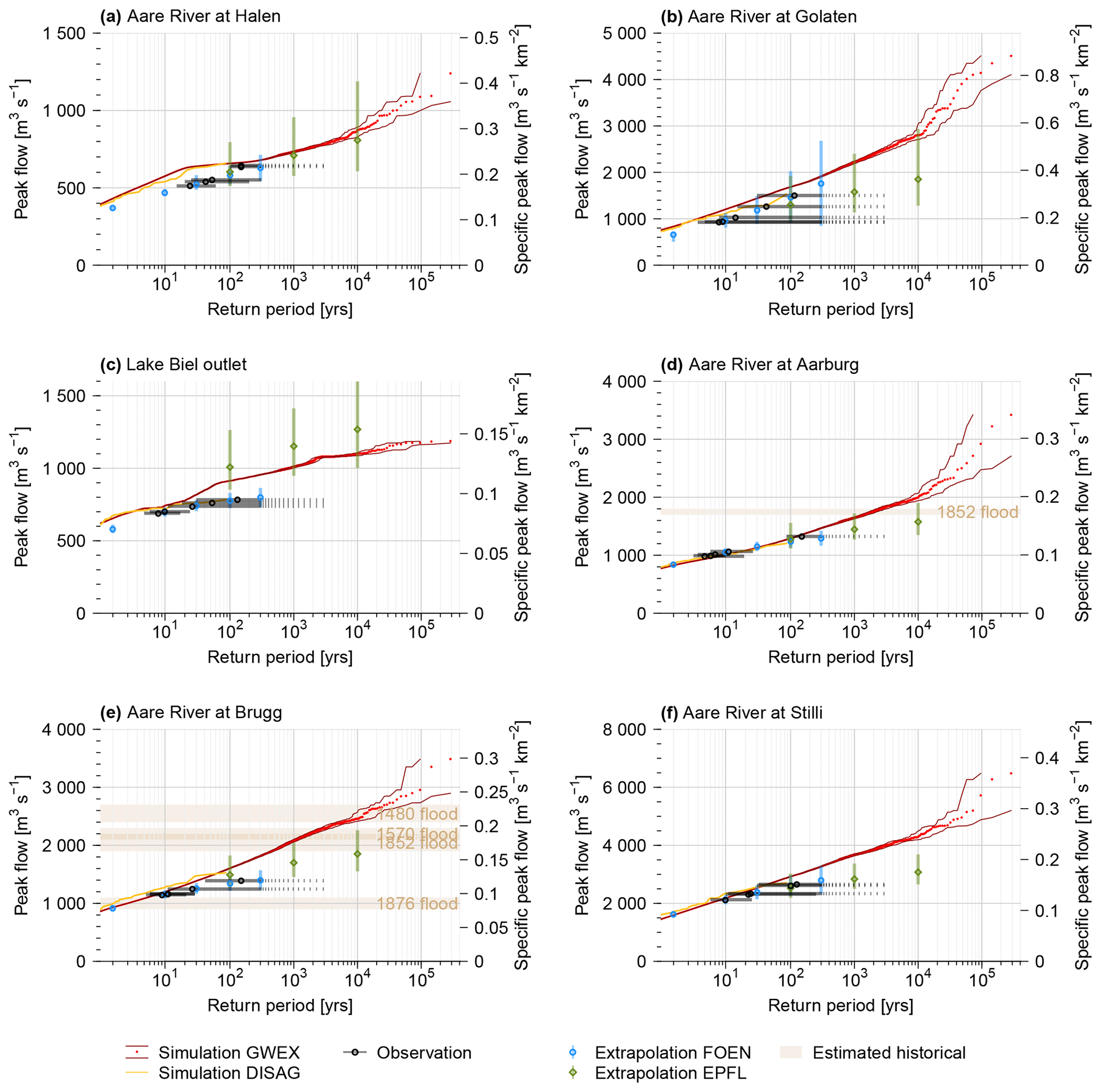
Figure 7Exceedance curves for selected sites along the Aare River: Halen, Golaten (downstream of the confluence with the Saane River), the outlet of Lake Biel (close to Brügg–Aegerten), Aarburg (downstream of the confluence with the Emme River), Brugg (upstream of the confluence with the Reuss and Limmat rivers) and Stilli (downstream of the confluence with the Reuss and Limmat rivers). Red: AMFs for CS (median representative parameter set) based on 289 000 years of GWEX weather scenarios, with the central 95 % confidence interval computed according to Loucks and van Beek (2017); orange: simulated AMFs (median representative parameter set) on the basis of 85 years of disaggregated weather observations (DISAG); black: five highest observed peak flows plotted at return periods according to FOEN with confidence interval (Baumgartner et al., 2013) (confidence intervals that are unbounded towards high return periods are dashed); blue: extrapolation of observed peak flow records according to FOEN with confidence interval (Baumgartner et al., 2013); green: regionally enhanced extrapolation of observed peak flow records according to EPFL with confidence interval (Asadi et al., 2018); light brown (for Brugg and Aarburg only): range of reconstructed historical floods (Baer and Schwab, 2020). Observation and reconstruction sites do not always match simulation sites exactly; the corresponding values have been scaled where necessary, assuming constant discharge per unit area.
4.4.3 Spatial patterns of the largest events
For an overview of spatial variability in extremes in meteorology and hydrology, Fig. 8 maps the conditions present in the 10 generated events that lead to the highest peak discharges at the outlet of the Aare River basin. The data refer to GWEX scenarios (Fig. 8a) and corresponding HBV simulations (Fig. 8b) for the 80 sub-catchments. For the 72 h cumulative precipitation scenarios (Fig. 8a), a relatively large range of conditions is found. The two largest hydrological events show a widespread occurrence of high precipitation sums with a slight emphasis on the central and eastern parts of the basin. Most of the other top-10 events have a stronger emphasis on parts of the basin where the region of emphasis varies. Simulated specific peak discharge (Fig. 8b) shows stronger and more homogeneous regional accents, but still a variety of spatial patterns. Values are often somewhat lower in the southern and southeastern parts of the basin. Contributions from these regions to peak discharges downstream are strongly attenuated by the pre-alpine lakes Brienz, Lucerne, Thun and Zurich. Therefore, the highest peak discharges simulated downstream in the Aare River (and presented here) are not caused by large events upstream of the pre-alpine lakes, and in turn, the events with high peak discharges upstream are not well represented in the events selected here.
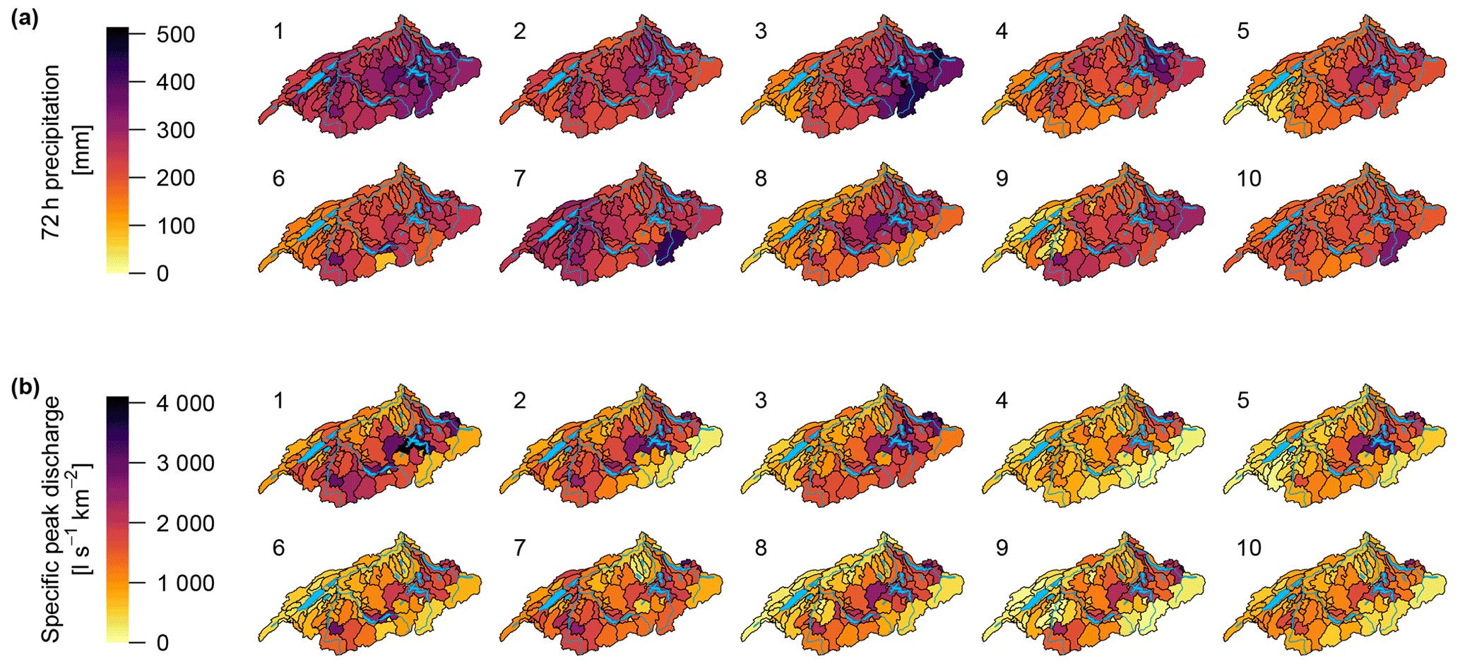
Figure 8Patterns of cumulative precipitation (maximum 72 h sum) (a) and specific peak discharge (b) for the 10 largest peak flow events simulated at the outlet of the Aare River basin. For return periods estimates, see Fig. 11.
Many of the simulated top-10 events have contributions of snowmelt runoff (Fig. 9a), mainly originating from the alpine area in the southern and southeastern part of the Aare River basin. In the extreme events studied here, notable snowmelt is possible even in July or August. Weighted over all sub-catchments, the ratio of snowmelt runoff volume to total runoff volume in the 72 h preceding peak flow at the Aare River outlet was between 7 % and 31 % in the 10 events studied here, with snowmelt runoff from the sub-catchments ranging between 3 and 19 mm (median: 11 mm). Alpine sub-catchments located in the south and southeast occasionally reached ratios of more than 60 %. As mentioned above, however, runoff from these sub-catchments is strongly attenuated by the pre-alpine lakes. The ratios were much smaller in the Swiss Plateau, with the exception of event 5. The average ratio of snowmelt runoff volume (72 h preceding peak runoff at the outlet) to maximum 72 h precipitation during the top-10 events was between 1 % and 13 % and showed slightly more diverse patterns than the ratio of snowmelt to total runoff volume.
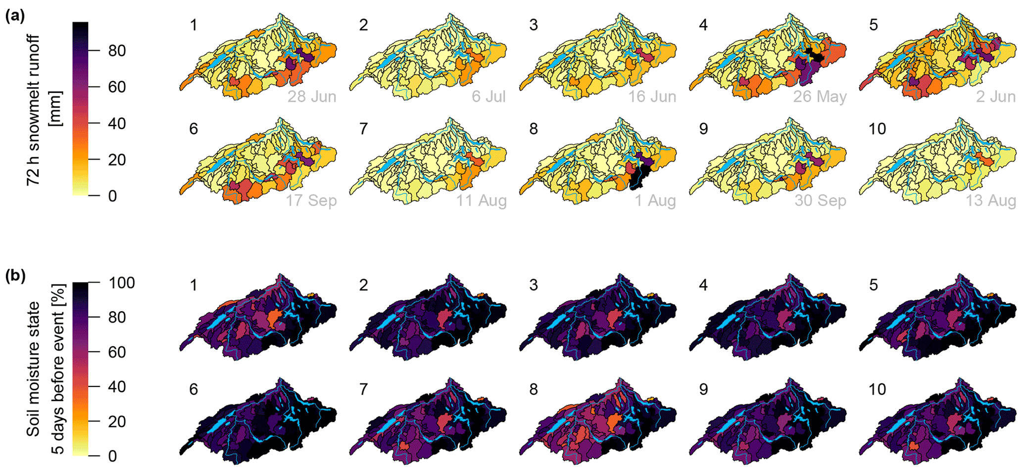
Figure 9Patterns of snowmelt runoff (sum over the 72 h preceding peak flow at the Aare River basin outlet) (a) and soil moisture storage (filling level relative to maximum storage available, 5 d before peak flow at the Aare River basin outlet) (b) for the 10 largest peak flow events simulated at the outlet of the Aare River basin.
To examine antecedent conditions, the status of simulated soil moisture was assessed. Here, we considered simulated soil moisture relative to maximum storage. It is important to note that maximum storage is a parameter of HBV and not necessarily equal to measured values of field capacity. Some variability can be noted 5 d before peak flow at the outlet (Fig. 9b), although the large precipitation amounts then led to extensive saturation in the following days. At the time of peak flow at the Aare River outlet, 9 out of 10 sub-catchments had filling levels of 85 % or more, and averaged over the entire basin, the filling levels ranged between 90 % and 95 % for the individual events. The limited variability at the time of peak flow at the outlet is not surprising because here we study the largest events, which are indeed caused by a combination of high soil moisture (i.e. high runoff ratio) and large precipitation amounts. By design of the CS approach, however, the broad spectrum of floods simulated also encompasses events with high saturation from considerable antecedent precipitation but moderate precipitation amounts during the event, as well as events with moderate saturation but large precipitation amounts.
5.1 Diversity of critical hydrometeorological configurations
A strong benefit of the multi-site, long-term hydrometeorological CS approach is the possibility for exploring a vast diversity of hydrometeorological configurations and to generate critical combinations of initial hydrological state patterns and weather dynamics, including combinations that can generate very rare floods. This benefit is particularly relevant when a large river basin is the focus, as in our case. Due to the large spatial extent, the number of tributaries and the complexity of hydraulic conditions, a wide variety of combinations is possible regarding hydrometeorological states and dynamics. However, this variety will hardly be reflected in observations, since these only provide a comparatively short, arbitrary and thus most likely unrepresentative sample.
The diversity of configurations simulated by the weather generator is illustrated with the severity maps of precipitation in Fig. 10. These maps present the GWEX-generated precipitation amounts of the 10 largest peak flow events at the Aare River outlet. In detail, they report the return periods of cumulative precipitation amounts for all sites considered, as well as for different spatial and temporal scales over the 30 d preceding the flood peak at the Aare River outlet. The largest peak discharge event is clearly triggered by a very large precipitation event, with the corresponding return periods exceeding 100 000 years for accumulation durations from 2 to 7 d in most of the Aare River basin (Fig. 10a). Figure 10b shows that the spatial and temporal variety of triggering precipitation is indeed very large, and the critical regions as well as the critical accumulation durations vary substantially between events. This highlights that aside from precipitation, other factors (such as the coincidence of floods from different sub-regions) are also important for the generation of the extreme floods simulated.
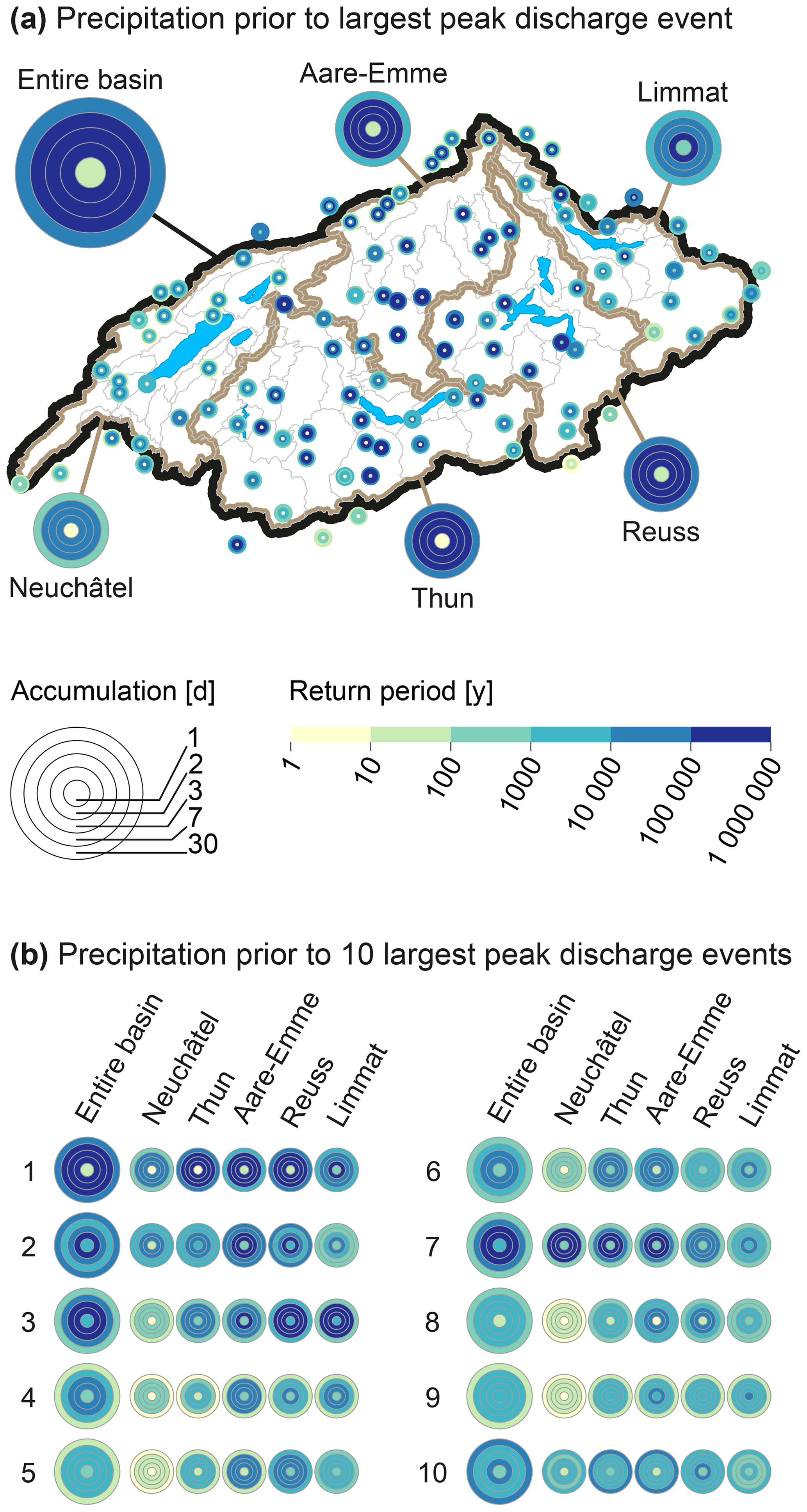
Figure 10Return periods of precipitation over different accumulation durations (in days before occurrence of peak discharge at the Aare River outlet), shown for all sites considered (only for largest hydrological event in panel a) as well as for different spatial aggregations (sub-regions and entire basin) for the 10 biggest peak flow events simulated at the outlet of the Aare River basin (panel b).
Further severity maps are available in Staudinger and Viviroli (2020), also covering the five largest 1 and 3 d GWEX precipitation events as well as all similar maps for SCAMP-generated precipitation. Analysis of these maps confirms that for both GWEX and SCAMP, a large variety of spatial and temporal dynamics were generated, consistent with the variety of events present in the observation period and beyond, exploring different combinations of antecedent precipitation and event precipitation severity. While it was not possible to check the realism of these maps quantitatively, a visual analysis together with experts from MeteoSwiss did not reveal unrealistic patterns.
For the entire model chain, spatial patterns of the top-10 hydrological events were shown in Fig. 8. However, this display partly masks the variety of conditions because precipitation, specific peak discharge and snowmelt runoff have inherent patterns due to climatological differences between the plateau, Jura, pre-alpine and alpine areas (see e.g. Isotta et al., 2014). These climatological differences can be removed by considering return periods instead of amounts, as was already done in the severity maps for precipitation above (Fig. 10). These return periods (Fig. 11) reveal a considerable variety also for the hydrological patterns. Note that a map for snowmelt and soil moisture return periods is not provided because the simulated state variables were only stored for the events selected due to the large disk write time and storage costs.

Figure 11Patterns of return periods for cumulative precipitation (maximum 72 h sum, using Gringorten plotting position) (a) and specific peak discharge (using Weibull plotting position) (b) for the 10 largest peak flow events simulated at the outlet of the Aare River basin. For absolute values, see Fig. 8.
Overall, the largest floods in the generated time series came from very different hydrometeorological configurations: some of the floods were caused by huge precipitation amounts falling over the whole Aare River basin for 1 or 2 d preceding the flood peak; some were caused by heavy precipitation concentrated on smaller, varying parts of the Aare River basin; and some were caused by precipitation falling over a few days preceding the flood peak. The emerging patterns of peak flows in the individual sub-catchments are similarly diverse and essentially follow the patterns of 72 h cumulative precipitation, with some differences due to the varying spatial and temporal dynamics of the precipitation scenarios and varying contributions of snowmelt.
5.2 Realism of resulting floods
Although the present CS chain relies on state-of-the-art models parameterized with robust regional approaches and estimation methods, its results need to be assessed and checked in some way. This concerns both the plausibility of the large flood events obtained and the return periods estimated from the exceedingly long CS. In the following we compare the results of the CS chain to observations and estimates obtained from previous work in the region. Although a strict comparison is not possible for different reasons mentioned below, this analysis is nevertheless informative.
5.2.1 Full exceedance curve
Overall, the full exceedance curves of AMFs from the hydrometeorological model chain (Fig. 7) compare well with standard statistical extrapolations of observed data (Baumgartner et al., 2013), as well as extrapolations enhanced with a regional statistical model (Asadi et al., 2018). At Halen (Fig. 7a), the most upstream site considered in the Aare River, the discrepancy for events with a return period of less than 100 years is explained by a flood discharge tunnel that was completed in 2009. While this tunnel is represented in the model, it affects only the last few years of streamflow observations and is thus only marginally represented in the extrapolations. Roughly 17 km downstream at Golaten (Fig. 7b), the simulations yield higher AMFs than observations and extrapolations across all return periods, mainly because of the inflow of the Saane River immediately upstream. In comparison to observations, the Saane River shows noticeably higher simulated AMFs from the full CS, even though simulated AMFs from using the disaggregated meteorology of 1930–2014 agree well with observations. Downstream of the Jura lake system (lakes Biel, Murten and Neuchâtel; see Fig. 2), the simulations show higher AMFs for return periods considerably larger than 100 years. Here, the model can simulate a failure of the Jura lake system, which would lead to a reactivation of the original bed of the Aare River and a bypassing of the three Jura lakes. In such an event, the flood peak in the Aare River downstream of Lake Biel would arrive considerably faster and more pronouncedly. This bypassing would occur at a discharge of around 1880 m3 s−1, which is higher than the maximum of 1514 m3 s−1 recorded in 2005 and is thus not represented in discharge records and extrapolations thereof. In a similar vein, the highly nonlinear response of the three lakes and their interplay with widespread inundations during extreme events is poorly sampled by the records. At Stilli (Fig. 7f), downstream of the confluence of the Aare (surface area at this location: 11 708 km2), Reuss (3426 km2) and Limmat (2412 km2) rivers, the discrepancy for rare and very rare floods is likely due to unfavourable configurations of weather events that are inadequately sampled in the streamflow observations. Although the flood peaks from the Aare, Reuss and Limmat rivers did arrive in a relatively narrow time window of less than 10 h in some of the largest observed events (e.g. 1994, 2005 and 2007), only one of the three individual rivers showed a flood with a return period exceeding roughly 50 years in all of these events.
As an important context for the above juxtaposition of simulated and observed values, it should be emphasized that results of the CS chain are not directly comparable to statistics of observed discharge for several reasons. First, observations of annual maximum discharge have limited length (here between 32 and 112 years), and extrapolations are usually not recommended for return periods of more than 100–300 years due to the large uncertainties (Maniak, 2005; Baumgartner et al., 2013). Second, many streamflow records are inhomogeneous due to hydraulic structures and diversions built over the decades. One of the most important examples in the Aare River basin is the second Jura Water Correction of 1962–1973 (Vischer, 2003). This correction led to slightly higher values for frequent AMFs downstream of Lake Biel. Consequently, the extrapolation for less frequent floods gives slightly higher values as well (see Klemeš, 1986, for the impact of low values on the upper tail of a probability distribution). This inconsistency has been eliminated from the FOEN flood statistics by dismissing years before 1974 (Bundesamt für Umwelt, 2020). By contrast, it is not feasible to eliminate the impact of the many further, smaller alterations. Third, for a large river basin such as the Aare, flood configurations can derive from a multiplicity of specific hydrometeorological configurations, as already mentioned. Many of those configurations have not yet been observed. The observational period is thus much too small to provide a representative sample of possible hydrometeorological configurations. It is expected that this poor representativity is reduced with the flood sample obtained from long CS. Indeed, CS essentially exploits precipitation and temperature records (here with a length of 85 years) at multiple sites to parameterize a multi-site weather generator and to enable exceptionally long hydrological simulations that are finally evaluated statistically. The extrapolation to small probabilities is thus based on meteorological rather than hydrological observations, and therefore a considerably broader range of conditions can be covered than is present in the streamflow records. This concerns especially the extent, spatial configuration and temporal progress of triggering meteorological events, and the combined hydrological response of the many sub-catchments (see previous section). All in all, there is no reason to expect a perfect statistical correspondence between observations and simulations.
Results of CS have also been compared to selected historical flood events of the past 540 years in the region. At all sites where it is possible to reconstruct such historical events (Table 1), the largest simulated AMFs exceed the reconstructed peaks clearly (see examples for the Aare River at Aarburg in Fig. 7d and at Brugg in Fig. 7e). Again, reconstructed historical and current flood peaks should only be compared with due care. On the one hand, major changes have been made to the river network over the past centuries. Under today's conditions, the peak values of historical floods would have a smaller probability, mainly because of the diversions of the Aare River into Lake Thun (1714) and Lake Biel (1878). These diversions have been made to exploit lake retention and thus attenuate flood peaks under present conditions. On the other hand, long-term internal climate variability over timescales of decades to centuries is likely to have impacted flood frequencies (Redmond et al., 2010). In northern Switzerland, four periods rich in floods occurred since 1500, lasting roughly between 30 and 100 years each. The current period rich in floods started in 1970, and the previous such period occurred in 1820–1940 (Schmocker-Fackel and Naef, 2010a). In the CS approach used here, the low-frequency fluctuations in large-scale atmospheric circulation underlying the flood-rich and flood-poor periods (Schmocker-Fackel and Naef, 2010b) have not been accounted for by the weather generators, limiting in turn the comparability of return periods.

Figure 12Range of the top-10 flood peaks simulated based on GWEX scenarios with the median representative parameter set for each output node of the Aare River system (RS MINERVE output, red) and each sub-catchment (HBV output, orange), in comparison to observed and reconstructed peak discharges (Eidgenössisches Amt für Strassen- und Flussbau, 1974; Kienzler and Scherrer, 2018), separately for the Aare River basin (dark blue), the Rhine River basin (without sites in the Aare River basin) (medium blue) and the rest of Switzerland (light blue). For orientation, enveloping curves are shown for the Rhine River basin (Vischer, 1980, here including the Aare River basin; valid for catchments with an area of up to roughly 10 000 km2), Europe (Marchi et al., 2010) and the world (Herschy, 2002).
Keeping in mind these limitations, the realism of the highest floods simulated at all sites considered is assessed in Fig. 12 in comparison to the comprehensive records of large observed and reconstructed flood peaks in Switzerland (Eidgenössisches Amt für Strassen- und Flussbau, 1974; Kienzler and Scherrer, 2018). These records date back to 1342, and the earliest record for the Aare River basin is from 1629. Maximum peak discharges from CS are higher than the recorded floods in the Aare River basin for catchment areas of more than roughly 1000 km2, with a factor of about 2 for the largest catchments simulated. At some sites, the simulations exceed the enveloping curve for maximum discharge in the Rhine River basin estimated by Vischer (1980) on the basis of data from Eidgenössisches Amt für Strassen- und Flussbau (1974). However, they are still within the range of maximum discharges recorded in other parts of Switzerland. The fact that simulated flood peaks fall noticeably below the top of the point cloud for catchments with an area of less than 100 km2 indicates that indeed the set-up of the weather generator and the hourly time step are not suitable for estimating rare-flood peaks in individual smaller catchments, where short convective events typically lead to maximum discharge. As noted in Sect. 3.3.2, results should only be interpreted for catchments with an area of more than 1000 km2. At that scale, the comparatively lower values from small catchments are not relevant, as rather the interplay of these catchments in reaction to precipitation events lasting a few days becomes decisive. All values simulated lie well below the enveloping curves for Europe (Marchi et al., 2010) and the world (Herschy, 2002). However, these comparisons have limited validity due to large differences in climatological and hydrological conditions.
5.2.2 More frequent floods
One of the main advantages of long-term CS with a hydrometeorological model chain is that it not only provides information about peak flows with a small probability but can also lead to consistent results for more frequent floods as is often required in engineering and spatial planning. To examine the validity of our results in this respect, we subdivided the full CS into blocks that, in length, correspond to the length of the observed peak flow record at the site examined (e.g. Aare at Stilli: 2580 blocks with a length of 112 years) (Fig. 13). Comparison with observed floods shows high agreement for the Aare River at Aarburg (Fig. 13a) and the Limmat River outlet (Fig. 13c). At Aare–Aarburg, between 4 % and 7 % of the 100-year simulation blocks exceeded the range reconstructed for the historical flood of 1852. For the Reuss River outlet (Fig. 13b) and the Aare River at Stilli (Fig. 13d), the bulk of the simulation blocks reach higher floods than the observations. However, the observed peaks still fall within the confidence intervals of the simulation blocks. The simulations using disaggregated precipitation and temperature from 1930–2014 agree well with observations and CS.
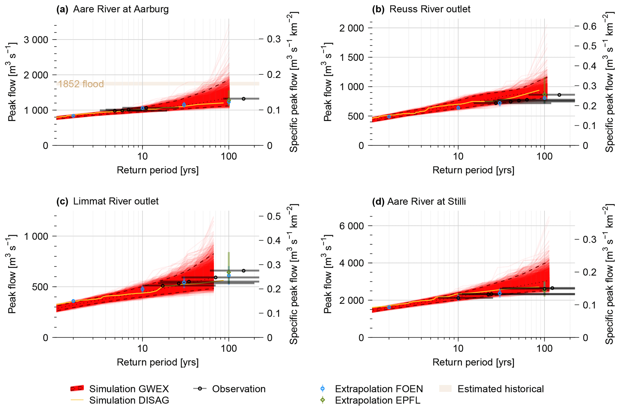
Figure 13Exceedance curves for AMFs from 289 000 years of CS based on GWEX weather generator scenarios (red), split up into blocks with length equal to that of observed peak flow records. Results are shown for the Aare River at Aarburg (a, block length of 100 years), the outlets of rivers Reuss (b, 106 years) and Limmat (c, 65 years), and for the Aare River close to the outlet at Stilli (d, 112 years). Orange: AMFs from 85 years of simulation (median representative parameter set) using disaggregated weather observations for 1930–2014 (DISAG); black: top-five observed peak flows drawn at return periods estimated by FOEN (Baumgartner et al., 2013); blue: extrapolation of observed peak flow records by FOEN (Baumgartner et al., 2013); green: regionally enhanced extrapolation of observed peak flow records according to EPFL (Asadi et al., 2018); light brown (for Aare at Aarburg only): range of reconstructed historical floods (Baer and Schwab, 2020). Measurement sites do not always match simulation sites exactly; the corresponding observations and extrapolations have been scaled where necessary, assuming constant discharge per unit area.
In this context, it is important to remember that only the recorded peak flow is an observation (albeit subject to measurement errors and uncertainty in the stage–discharge relationship; see e.g. Westerberg et al., 2020), whereas the corresponding return period – and thus the position on the abscissa – is a statistical estimate. If the uncertainty in the return period estimate is considered (horizontal bars drawn with observations in Fig. 13), there is a large overlap between the confidence intervals of observations and CS also for the Aare River at Stilli. As was the case with rare to very rare floods (previous section), the slight disagreement between GWEX-based simulations, disaggregation-based simulations and extrapolations of discharge observations is not surprising due to the limited length, representativity and homogeneity of the flood records, as well as due to slightly different reference time periods.
5.3 Differences between GWEX-based and SCAMP-based simulations
As a further check of plausibility, the SCAMP hybrid weather generator based on atmospheric and weather analogues was used as an alternative for the first link of the model chain. SCAMP is structurally independent from GWEX and makes use of additional variables stemming from an atmospheric reanalysis (see Sect. 3.2.2). A full set of 30 scenarios with 10 000 years of hourly data was produced in SCAMP and evaluated meteorologically (see Sects. 4.1 and 5.1). Since it was not possible to process all of these data with the hydrological model and routing due to high computational cost, 3425 years containing the largest precipitation events were sampled from the SCAMP scenarios (see Sect. 3.3.2) and then run through HBV and RS MINERVE. Note that the event sampling did not systematically consider contributions of snowmelt and that it is therefore not possible to make robust estimates regarding the return periods of the ensuing hydrological events. Furthermore, the largest meteorological events do not necessarily lead to the largest hydrological events. Comparison of the simulations using selected SCAMP scenarios with the full simulations using all GWEX scenarios could thus be misleading. The evaluation was therefore limited to the 10 largest discharge events resulting from SCAMP- and GWEX-based simulations, respectively.
Although SCAMP and GWEX are methodologically fully independent from each other, their largest precipitation events led to simulated floods in a similar order of peak magnitude (Fig. 14). In the individual HBV sub-catchments, SCAMP generally led to slightly higher peak discharges than GWEX; this difference was smaller in large sub-catchments. Simulation results after hydrological routing compare equally well, also with a tendency of SCAMP scenarios leading to slightly higher peak flows in comparison to GWEX scenarios. The seasonality of the 10 largest events is limited to May–October using GWEX and to May–November using SCAMP. GWEX shows a slight skew towards June–August, and SCAMP shows one towards August–October. These differences are at least partly explained by the constraint that only a subset of SCAMP events could be examined and that the selection of this subset has some limitations as noted before.
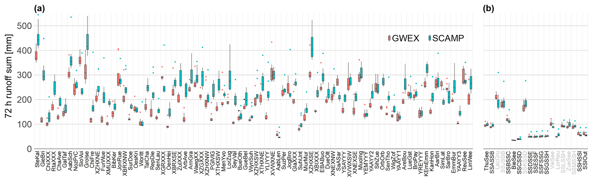
Figure 14Comparison of hydrological results achieved with GWEX inputs (red) and SCAMP inputs (blue). Shown are boxplots for the 10 largest 72 h runoff sums (median representative parameter set), each for the outlets of the 80 individual HBV sub-catchments (a: ordered by increasing catchment area) and the 19 RS MINERVE nodes (i.e. critical sites including the Aare River outlet) (b: ordered by location along the Aare River; tributaries are designated with a grey label colour). For the sub-catchment and output node abbreviations, see Tables S2 and S3.
5.4 Comparison to PMP–PMF approach
The so-called PMP–PMF method is popular in many countries as a basis for safety assessments of dams and critical infrastructure. In this method, the estimated probable maximum precipitation (PMP) of a certain duration serves to estimate an associated probable maximum flood (PMF) (Kienzler et al., 2015; Felder and Weingartner, 2017). Several methods for making PMP–PMF estimates have been proposed, but there is no scientific consensus about a preferred method. Large uncertainties are inherent in PMP and PMF estimates, e.g. due to the parameterization of the numerical atmospheric and hydrological models used to simulate them or due to assumptions regarding the simulated atmospheric configuration and the antecedent saturation configuration of the catchment. It is thus generally recommended to evaluate their plausibility by comparison to results from other methods. In recent publications, the PMP–PMF method was applied to Swiss catchments of different sizes and characteristics, e.g. to the Aare River upstream of Bern (Felder and Weingartner, 2016, 2017; Zischg et al., 2018), the Kander River upstream of Hondrich (Felder et al., 2019), the Emme River upstream of Wiler (Felder et al., 2019) and the Sihl River upstream of Zurich (Kienzler et al., 2015). In all of these studies, the PMP estimates have been distributed in time and space and then run through the hydrological model PREVAH (Viviroli et al., 2009a) to arrive at PMF estimates. Except for the Sihl River study, a 1D hydrodynamic model was used as a last step to account for effects of overbank flow and to achieve a more realistic routing.
All these PMF values are based on methods substantially different from the ones employed here, and it is not possible to determine an exact return period for them. However, they are in a similar order of magnitude as the maximum peak flows from CS based on GWEX scenarios (Table 2). For the Aare River at Bern and the Emme River, values are even very similar, whereas differences are a little larger for the Kander and Sihl rivers. The latter two have a comparatively small surface area and are therefore more sensitive to differences in precipitation configuration present between temporally and spatially redistributed PMP values and weather generator outputs. Moreover, it has to be kept in mind that GWEX was developed with a focus on larger regions (area of roughly 1000 km2 or more) and thus for combinations of the sub-catchments used in the present study. Peak flow results from single sub-catchments should only be interpreted with the greatest care. On the other hand, the PMP maps elaborated for Switzerland cannot be used to derive PMFs for large catchments: in these maps, the PMP estimates reported for the different locations of a given area often result from different large-scale atmospheric configurations that are highly unlikely to occur at the same time. For example, the 24 h PMP in the southern part of the Swiss Alps is a compound of wind flow from the southwest to the southeast, whereas in the northern part it is a compound of wind flow from the west, northwest, northeast and east. In addition, the upper recommended spatial scale for use of the PMP–PMF estimates is a few hundred square kilometres (e.g. 230 km2 for Fallot et al., 2017). Notwithstanding, the rough agreement between the PMP–PMF estimates available and results of the CS approach strengthens confidence in view of the fundamental methodological differences. Results from using SCAMP scenarios are not available here because the selection of events focused on peak flow values at the outlet of the Aare River basin; this selection does not cover the largest events in individual smaller sub-catchments.
Table 2Probable maximum flood (PMF) estimates reported in the literature that apply to the perimeter covered in the present study and corresponding maximum peak flows from CS based on GWEX (Qmax,GWEX).
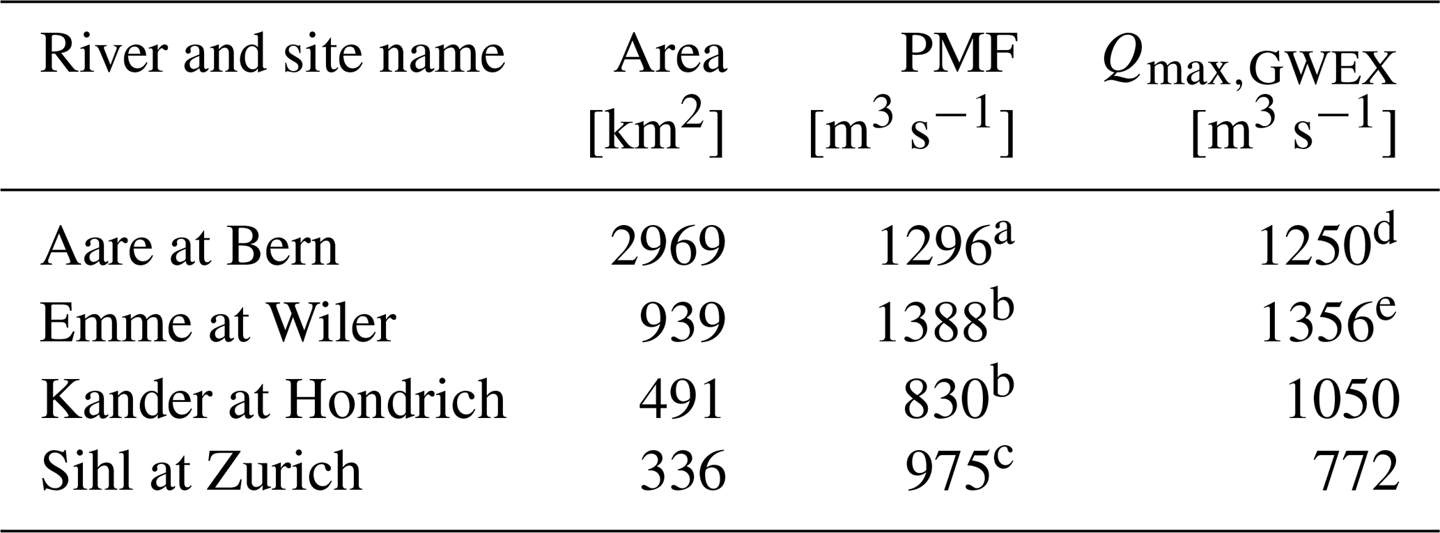
a Felder and Weingartner (2016, 2017), Zischg et al. (2018); b Felder et al. (2019); c Kienzler et al. (2015); d results for the Aare River at Halen, which compares well to Aare at Bern (see Table S3); e results for the Emme River outlet, which compares well to Emme at Wiler (see Table S3).
5.5 Uncertainties and limitations
The CS approach as implemented here is subject to several uncertainties and limitations. These mainly stem from structural and parameter uncertainties in the weather generator, the hydrological model and the hydrological routing; the limited length of the observations; measurement errors especially in precipitation and discharge; and uncertain stage–discharge relationships. In addition, the approach assumes that key characteristics of the model chain – such as the spatial dependence structure of large precipitation events – are also valid for extreme events well beyond the observed range.
While selected aspects of these uncertainties have been briefly discussed above and are described in more detail elsewhere (e.g. Sikorska-Senoner and Seibert, 2020; Staudinger and Viviroli, 2020; Westerberg et al., 2020; Andres et al., 2021; Sikorska-Senoner, 2022), a full quantification of uncertainties propagated through the model chain was not feasible due to the enormous computational cost of a comprehensive analysis.
When it comes to large simulated discharge extremes in the present domain and scale, the behaviour of the weather generators GWEX and SCAMP has a major impact on results. As a basis for the parameterization of the two generators, it was possible to use a high-quality dataset of meteorological records with a maximum duration of 85 years since 1930. Both length and spatial coverage of this dataset are exceptional in comparison to other regions and allowed for a very robust estimation of the weather generator parameters. However, for the domain of the highest extremes the length of the records is still limited and permitted only a partial evaluation of results. In particular, this limits knowledge of the spatial covariance between local extremes. Within the methods employed here, potentially better model configurations could only be found with considerably longer records, which is unrealistic. However, the comparison of peak flow results based on the two methodologically fully independent weather generators suggests that structural choices are not decisive.
Concerning the temporal disaggregation of the weather scenarios from a daily to an hourly scale, an obvious limitation is related to the limited observations available at the hourly scale. As a result, for instance, disaggregated fields might miss the spatiotemporal dynamics of localized precipitation events (e.g. convective storms). For temperature, the inclusion of additional predictors such as the daily temperature field or a preselection of the analogue dates based on a seasonal filter or an atmospheric circulation model could also be considered possible refinements. Nevertheless, it is also important to note that this disaggregation approach is stochastic, which partly handles the uncertainties related to this postprocessing step. Indeed, for both GWEX and SCAMP, the spatiotemporal field used for the disaggregation is that of an analogue day, which was randomly drawn from a set of analogue candidates.
Regarding hydrological modelling and routing, it should be mentioned that structural uncertainty can surmount parameter uncertainty (Vrugt et al., 2003; Kavetski et al., 2006; Schaefli et al., 2007; Sikorska and Renard, 2017). For reasons of computational cost, it was only possible to quantify parameter uncertainty at individual sub-catchments and provide analyses on stage–discharge uncertainty at selected sites (Westerberg, 2020; Westerberg et al., 2020). However, high runoff coefficients can be expected for rare to very rare flood events like the ones in focus here, and consequently the magnitude of simulated precipitation (including associated uncertainties) is likely more decisive than the hydrological model structure. In addition, we propagated the three representative parameter sets of the hydrological model through to the hydrological routing. These sets are intended to represent the prediction interval due to parameter uncertainty in the hydrological model (Sikorska-Senoner et al., 2020) at individual sub-catchments. However, the cumulative effect of uncertainty propagation through the model chain at different sites along the major rivers is difficult to assess due to its nonlinearity, particularly because different uncertainty sources may dominate the simulation uncertainty at different sites.
In addition, the peak flow estimates do not distinguish between different flood-governing processes such as rainfall-driven or snowmelt-driven floods (Merz and Blöschl, 2003; Diezig and Weingartner, 2007; Sikorska et al., 2015). Flood estimates adapted to specific flood types might improve the realism of the results, but this issue would require further research.
CS is a valuable option for estimating rare to very rare floods at multiple sites in a large river basin. Compared to statistical approaches based on streamflow observations, the CS approach has substantial advantages in that it explicitly considers important processes of flood generation such as soil moisture, snow accumulation and snowmelt, and in addition it can implement lake regulation and dam operation as well as lake and floodplain retention. Even more importantly, the large diversity of possible but not observed temporal and spatial hydrometeorological configurations (for both antecedent conditions and weather forcing sequences) covered by the simulations provides considerable extra information on the magnitude of floods with a certain return period. This enables the identification of critical hydrometeorological configurations that could not have been found with a simple a priori guess of a so-called design configuration obtained from relating a design weather event with an assumed initial catchment state.
For return periods larger than roughly 1000 years, the flood peaks simulated for multiple sites in the Aare River basin are slightly higher than what could be expected from a frequency analysis of discharge observations. This disagreement, however, is not surprising due to the limited length, representativity and homogeneity of the flood records. A comprehensive assessment of the simulations has not revealed important shortcomings, and plausible explanations were found for the disagreements. Also, the application of two structurally independent weather generators has shown comparable hydrometeorological results, which increases confidence in the flood estimates.
Despite the advantages of the CS-based flood estimation presented here, it should be kept in mind that results are still subject to considerable uncertainties. These are largely due to the limited length of meteorological and hydrological observations available and can thus not be fully amended with additional computational resources and a higher number of simulated scenarios.
The wealth of hydrometeorological scenarios available from long-term CS at multiple sites in a large river basin opens up some interesting possibilities. We demonstrated that the present implementation is indeed not only useful for estimation of rare to very rare floods but also dependable for floods with return periods clearly lower than 1000 years. There, long-term CS at multiple sites can be used as an alternative approach to flood estimation and complement the extrapolation of streamflow observations. In particular, CS results are not prone to inhomogeneities due to the relocation of streamflow gauges, changes in river network and hydraulic structures. However, CS, of course, contains its own specific set of uncertainties and limitations. Furthermore, flood estimates for the sites considered in CS are inherently consistent because they stem from the same meteorological scenario input. This consistency is important, e.g. for the comparability of hazard mapping over large areas, but is frequently not ensured because of the different record lengths at the relevant observation sites. The same advantages regarding consistency can be exploited for multivariate flood estimates, including flood volumes (e.g. Brunner et al., 2017) and exceedance times of flood levels, and for identifying relevant hydrograph shapes for different return periods, e.g. by processing the exceedingly long simulations with functional data analysis (Chebana et al., 2012; Ternynck et al., 2016; Staudinger et al., 2021). In this context, an extension of the methods towards small sub-catchments, e.g. 10 km2 or larger, would be highly desirable, since this scale range is even less well covered by streamflow observations. However, this would require considerable methodological adaptations to the weather generators used here. A particular challenge would be to ensure easy application over a wide spatial domain (e.g. all of Switzerland), avoiding time-consuming set-up and calibration procedures for individual catchments.
A multi-site CS implementation can also inform comprehensive flood risk assessments in a large river basin (see EXAR project, Andres et al., 2021). The abovementioned spatial consistency of results is a decisive advantage for this kind of assessment, and floods even less probable than the ones considered here can be estimated with a focus on critical infrastructure. Since extrapolation of CS results is not advisable due to the large uncertainties involved in the model chain, event tree analyses can be performed based on CS results, and return periods of 100 000–10 000 000 years can be examined (Dang and Whealton, 2020). For this, the hydrometeorological scenarios can be combined with 2D hydraulic simulations covering further relevant hazard scenarios (Pfäffli et al., 2020), including landslides, blockages of bridge openings by driftwood, bank erosion, failure of protective dikes, human failures (e.g. in weir regulation) and dam failures due to extremely rare earthquakes (Andres et al., 2021). Such event tree analyses are not possible on the basis of PMP–PMF or other approaches that do not include an estimate of the return period.
The weather generator is obviously a key component, enabling the exploration of a large variety of possible hydrometeorological configurations and their development into flood events. However, the choice and implementation of a suitable weather generator is also one of the most challenging issues in the CS approach (Lamb et al., 2016). Such a generator is subject to many requirements that may be difficult to satisfy: it has to produce relevant simulations across the whole continuum of weather situations from frequent precipitation events to extreme ones, including wet and dry spells; it has to cover extents ranging from localized to catchment-wide; it has to account for the dependence between weather event characteristics and weather types, likely calling for specific parameterizations; and it has – depending on the region – to address the specific challenges of simulating meteorological and hydrological processes in complex terrain. The development of such a generator is thus not straightforward, and more attention should be paid to this issue so that robust and relevant simulation tools can be made available for similar studies worldwide. The weather generators developed for this work are built on the latest and most advanced statistical models and developments available to date. If the rare weather scenarios generated for this work are thus very likely relevant from a statistical point of view, their physical relevance remains uncertain. An alternative to weather generators for rare events could be numerical atmospheric models, as they allow for a more physically based approach. Numerical atmospheric models are however not free of limitations either, as they are typically based on a number of simplifications, assumptions and parameterizations. A relevant estimate of critical weather events would also require intensive uncertainty analyses, likely difficult to achieve. More importantly then, the large computational cost of such models prevents the generation of corresponding long time series of weather scenarios. This in turn prevents an in-depth exploration of a large variety of hydrometeorological configurations – combining different spatial patterns of initial hydrological states and different dynamics of weather development and, in turn, the identification of critical hydrological configurations. Besides the uncertainties in the meteorological scenarios, the uncertainties in the hydrological simulations should also be examined more rigorously in future research. For large-scale applications like the one presented here, computational cost is again a restricting factor to date. The same applies to uncertainty evaluations that propagate from meteorological scenarios to hydrological modelling and routing.
Implementing the present CS for multiple sites in other large river basins is feasible as long as records of discharge, precipitation and temperature are available in sufficient length (ideally a few decades), as well as in appropriately high temporal (hourly) and spatial (see recommendations by World Meteorological Organization, 1994) resolution. However, the specific weather regimes and precipitation characteristics of other regions would likely require an adaptation of the weather generator to represent precipitation and temperature events that are critical for the region considered well.
Code used in this research can be obtained from the first author upon reasonable request.
The resulting data can be obtained from the first author upon reasonable request.
The supplement related to this article is available online at: https://doi.org/10.5194/nhess-22-2891-2022-supplement.
ACF, BH, DV, JS and RW conceptualized the project. AS, DR, GE, GN, JC, MK and MS developed and calibrated the model and ran the simulations. AS, CW, DR, DV, GN, GE, JC, MK and MS analysed the data and carried out the investigation. AS, CW, DR, DV, GE, GN, JC, MS and MK visualized the data. DV drafted the paper. ACF, AS, BH, CW, GE, GN, JS, MK and MS reviewed and edited the paper.
The contact author has declared that none of the authors has any competing interests.
Publisher's note: Copernicus Publications remains neutral with regard to jurisdictional claims in published maps and institutional affiliations.
This article is part of the special issue “Hydro-meteorological extremes and hazards: vulnerability, risk, impacts, and mitigation”. It is not associated with a conference.
We thank MeteoSwiss; FOEN; and the cantons of Aargau, Bern, Fribourg, St. Gallen, Vaud and Zurich for providing data to make this study possible. We also thank Peiman Asadi, Anthony Davison, Sebastian Engelke, Luise Keller, Thomas Lugrin and Marc Vis for their contributions. The ScienceCloud computational and storage infrastructure provided by Service and Support for Science IT (S3IT) at the University of Zurich enabled part of the computation-intensive simulations.
This research has been funded by the Swiss Federal Office for the Environment (FOEN), the Swiss Federal Nuclear Safety Inspectorate (ENSI), the Swiss Federal Office of Energy (SFOE), the Swiss Federal Office of Meteorology and Climatology (MeteoSwiss), and the Swiss Federal Office for Civil Protection (FOCP) as a part of the EXAR project (hazard information for extreme flood events on the rivers Aare and Rhine).
This paper was edited by Francesco Marra and reviewed by two anonymous referees.
Andres, N., Steeb, N., Badoux, A., and Hegg, C. (Eds.): Grundlagen Extremhochwasser Aare: Hauptbericht Projekt EXAR, Methodik und Resultate, WSL Berichte 104, WSL, Birmensdorf, https://www.wsl.ch/de/projekte/exar-1.html (last access: 12 August 2022), 2021.
Arnaud, P. and Lavabre, J.: Using a stochastic model for generating hourly hyetographs to study extreme rainfalls, Hydrolog. Sci. J., 44, 433–446, https://doi.org/10.1080/02626669909492238, 1999.
Arnaud, P. and Lavabre, J.: Coupled rainfall model and discharge model for flood frequency estimation, Water Resour. Res., 38, 1075, https://doi.org/10.1029/2001WR000474, 2002.
Arnaud, P., Cantet, P., and Odry, J.: Uncertainties of flood frequency estimation approaches based on continuous simulation using data resampling, J. Hydrol., 554, 360–369, https://doi.org/10.1016/j.jhydrol.2017.09.011, 2017.
Asadi, P., Engelke, S., and Davison, A. C.: Optimal regionalization of extreme value distributions for flood estimation, J. Hydrol., 556, 182–193, https://doi.org/10.1016/j.jhydrol.2017.10.051, 2018.
Aubert, Y., Arnaud, P., Ribstein, P., and Fine, J.-A.: La méthode SHYREG débit – application sur 1605 bassins versants en France métropolitaine, Hydrolog. Sci. J., 59, 993–1005, https://doi.org/10.1080/02626667.2014.902061, 2014.
Baer, P. and Schwab, S.: Extremhochwasser an der Aare: Detailbericht B Projekt EXAR, Historische Hochwasser, ARGE GEOTEST-HZP-IUB, Zollikofen, https://www.wsl.ch/de/projekte/exar-1.html (last access: 12 August 2022), 2020.
Baker, V. R.: Paleoflood hydrology: Origin, progress, prospects, Geomorphology, 101, 1–13, https://doi.org/10.1016/j.geomorph.2008.05.016, 2008.
Baker, V. R., Webb, R. H., and House, P. K.: The Scientific and Societal Value of Paleoflood Hydrology, in: Ancient floods, modern hazards: Principles and applications of paleoflood hydrology, edited by: House, P. K., American Geophysical Union, Washington, DC, 1–19, https://doi.org/10.1029/WS005p0001, 2010.
Barth, N. A., Villarini, G., and White, K.: Accounting for Mixed Populations in Flood Frequency Analysis: Bulletin 17C Perspective, J. Hydrol. Eng., 24, 04019002, https://doi.org/10.1061/(ASCE)HE.1943-5584.0001762, 2019.
Basso, S., Schirmer, M., and Botter, G.: On the emergence of heavy-tailed streamflow distributions, Adv. Water Resour., 82, 98–105, https://doi.org/10.1016/j.advwatres.2015.04.013, 2015.
Basso, S., Schirmer, M., and Botter, G.: A physically based analytical model of flood frequency curves, Geophys. Res. Lett., 43, 9070–9076, https://doi.org/10.1002/2016GL069915, 2016.
Basso, S., Botter, G., Merz, R., and Miniussi, A.: PHEV! The PHysically-based Extreme Value distribution of river flows, Environ. Res. Lett., 16, 124065, https://doi.org/10.1088/1748-9326/ac3d59, 2021.
Baumgartner, E., Boldi, M.-O., Kan, C., and Schick, S.: Hochwasserstatistik am BAFU – Diskussion eines neuen Methodensets, Wasser Energie Luft, 105, 103–110, 2013.
Bayliss, A. C. and Reed, D. W.: The use of historical data in flood frequency estimation, Centre for Ecology and Hydrology, Wallingford, Oxfordshire, UK, 92 pp., https://nora.nerc.ac.uk/id/eprint/8060/1/BaylissRepN008060CR.pdf (last access: 12 August 2022), 2001.
Ben Alaya, M. A., Zwiers, F., and Zhang, X.: Probable Maximum Precipitation: Its Estimation and Uncertainty Quantification Using Bivariate Extreme Value Analysis, J. Hydrometeorl., 19, 679–694, https://doi.org/10.1175/JHM-D-17-0110.1, 2018.
Benito, G. and O'Connor, J. E.: Quantitative Paleoflood Hydrology, in: Treatise on geomorphology, edited by: Shroder, J. F., Academic Press, London, Waltham, MA, 459–474, https://doi.org/10.1016/B978-0-12-374739-6.00250-5, 2013.
Benito, G. and Thorndycraft, V. R.: Palaeoflood hydrology and its role in applied hydrological sciences, J. Hydrol., 313, 3–15, https://doi.org/10.1016/j.jhydrol.2005.02.002, 2005.
Benito, G., Brázdil, R., Herget, J., and Machado, M. J.: Quantitative historical hydrology in Europe, Hydrol. Earth Syst. Sci., 19, 3517–3539, https://doi.org/10.5194/hess-19-3517-2015, 2015.
Bergström, S.: Utveckling och tillämpning av en digital avrinningsmodell, SMHI Notiser och preliminära rapporter, serie HYDROLOGI 22, SMHI, Norrköping, https://www.smhi.se/polopoly_fs/1.83595!/Menu/general/extGroup/attachmentColHold/mainCol1/file/Notiser_prel_rapporter_hydrologi_22.pdf (last access: 12 August 2022), 1972.
Bergström, S.: The HBV Model – its structure and applications, Reports Hydrology 4, Swedish Meteorological and Hydrological Institute (SMHI)/Sveriges Meteorologiska och Hydrologiska Institut (SMHI), Norrköping, https://www.smhi.se/polopoly_fs/1.83592!/Menu/general/extGroup/attachmentColHold/mainCol1/file/RH_4.pdf (last access: 12 August 2022), 1992.
Beven, K.: Towards the use of catchment geomorphology in flood frequency predictions, Earth Surf. Proc. Land., 12, 69–82, https://doi.org/10.1002/esp.3290120109, 1987.
Beven, K. J.: Rainfall-Runoff Modelling: The Primer, 2nd Edn. Wiley, Chichester, ISBN 978-0-470-71459-1, 2011.
Botter, G., Porporato, A., Rodriguez-Iturbe, I., and Rinaldo, A.: Basin-scale soil moisture dynamics and the probabilistic characterization of carrier hydrologic flows: Slow, leaching-prone components of the hydrologic response, Water Resour. Res., 43, W02417, https://doi.org/10.1029/2006WR005043, 2007.
Botter, G., Porporato, A., Rodriguez-Iturbe, I., and Rinaldo, A.: Nonlinear storage-discharge relations and catchment streamflow regimes, Water Resour. Res., 45, W10427, https://doi.org/10.1029/2008WR007658, 2009.
Breinl, K. and Di Baldassarre, G.: Space-time disaggregation of precipitation and temperature across different climates and spatial scales, J. Hydrol.: Reg. Stud., 21, 126–146, https://doi.org/10.1016/j.ejrh.2018.12.002, 2019.
Brunner, M. I., Viviroli, D., Sikorska, A. E., Vannier, O., Favre, A.-C., and Seibert, J.: Flood type specific construction of synthetic design hydrographs, Water Resour. Res., 53, 1390–1406, https://doi.org/10.1002/2016WR019535, 2017.
Buishand, T. A. and Brandsma, T.: Multisite simulation of daily precipitation and temperature in the Rhine Basin by nearest-neighbor resampling, Water Resour. Res., 37, 2761–2776, https://doi.org/10.1029/2001WR000291, 2001.
Bundesamt für Energie: Richtlinie über die Sicherheit der Stauanlagen: Teil C2: Hochwassersicherheit und Stauseeabsenkung, Richtlinie über die Sicherheit der Stauanlagen, 32 pp., https://www.bfe.admin.ch/bfe/de/home/versorgung/aufsicht-und-sicherheit/talsperren/richtlinien-und-hilfsmittel.exturl.html/aHR0cHM6Ly9wdWJkYi5iZmUuYW (last access: 12 August 2022), 2018.
Bundesamt für Umwelt: Stationsbericht Hochwasserstatistik Aare – Untersiggenthal, Stilli, https://www.hydrodaten.admin.ch/lhg/sdi/hq_studien/hq_statistics/2205_hq_Bericht.pdf (last access: 12 August 2022), 2020.
Bundesministerium für Land- und Forstwirtschaft, Umwelt und Wasserwirtschaft and Technische Universität Wien: Leitfaden zum Nachweis der Hochwassersicherheit von Talsperren, Wien, 107 pp., https://info.bml.gv.at/dam/jcr:4fd43e9f-c845-475e-ba34-62b4b25e9c60/Leitfaden_zum_Nachweis_der_Hochwassersicherheit_von_Talsperren_12_09.pdf (last access: 12 August 2022), 2009.
Burn, D. H.: Catchment similarity for regional flood frequency analysis using seasonality measures, J. Hydrol., 202, 212–230, https://doi.org/10.1016/S0022-1694(97)00068-1, 1997.
Calver, A. and Lamb, R.: Flood frequency estimation using continuous rainfall-runoff modelling, Phys. Chem. Earth, 20, 479–483, https://doi.org/10.1016/S0079-1946(96)00010-9, 1995.
Castellarin, A., Vogel, R. M., and Matalas, N. C.: Probabilistic behavior of a regional envelope curve, Water Resour. Res., 41, W06018, https://doi.org/10.1029/2004WR003042, 2005.
Castellarin, A., Kohnová, S., Gaál, L., Fleig, A., Salinas, J. L., Toumazis, A., Kjeldsen, T. R., and Macdonald, N.: Review of Applied European Flood Frequency Analysis Methods, COST Action ES0901, WG2, Wallingford, Oxfordshire, UK, 130 pp., ISBN 978-1-906698-32-4, 2012.
Chardon, J., Hingray, B., Favre, A.-C., Autin, P., Gailhard, J., Zin, I., and Obled, C.: Spatial Similarity and Transferability of Analog Dates for Precipitation Downscaling over France, J. Climate, 27, 5056–5074, https://doi.org/10.1175/JCLI-D-13-00464.1, 2014.
Chardon, J., Favre, A.-C., and Hingray, B.: Effects of Spatial Aggregation on the Accuracy of Statistically Downscaled Precipitation Predictions, J. Hydrometeorl., 17, 1561–1578, https://doi.org/10.1175/JHM-D-15-0031.1, 2016.
Chardon, J., Hingray, B., and Favre, A.-C.: An adaptive two-stage analog/regression model for probabilistic prediction of small-scale precipitation in France, Hydrol. Earth Syst. Sci., 22, 265–286, https://doi.org/10.5194/hess-22-265-2018, 2018.
Chardon, J., Evin, G., Favre, A.-C., Hingray, B., Nicolet, G., and Raynaud, D.: Weather Generators: GWEX and SCAMP, in: Extremhochwasser an der Aare: Detailbericht A Projekt EXAR, Hydrometeorologische Grundlagen, edited by: Staudinger, M. and Viviroli, D., University of Zurich, Zurich, 7–22, https://doi.org/10.5167/uzh-201388, 2020.
Chebana, F., Dabo-Niang, S., and Ouarda, T. B. M. J.: Exploratory functional flood frequency analysis and outlier detection, Water Resour. Res., 48, W04514, https://doi.org/10.1029/2011WR011040, 2012.
Dang, V. and Whealton, C.: Extremhochwasser an der Aare: Detailbericht G Projekt EXAR, Ereignisbaumanalyse und Gefährdungskurven, Paul Scherrer Institut, Villigen, https://www.wsl.ch/de/projekte/exar-1.html (last access: 12 August 2022), 2020.
Deutsche Vereinigung für Wasserwirtschaft, Abwasser und Abfall: Ermittlung von Hochwasserwahrscheinlichkeiten: DWA-Regelwerk, Merkblatt DWA-M 552, Hennef, 90 pp., ISBN 978-3-942964-25-8, 2012.
Diezig, R. and Weingartner, R.: Hochwasserprozesstypen – Schlüssel zur Hochwasserabschätzung, Wasser Abfall, 9, 18–26, https://doi.org/10.1007/BF03247473, 2007.
Eidgenössisches Amt für Strassen- und Flussbau: Die grössten bis zum Jahre 1969 beobachteten Abflussmengen von schweizerischen Gewässern: Beitrag zum internationalen hydrologischen Dezennium 1965–1974, EDMZ, Bern, http://permalink.snl.ch/bib/sz000413758 (last access: 29 August 2022), 1974.
England Jr., J. F., Cohn, T. A., Faber, B. A., Stedinger, J. R., Thomas Jr., W. O., Veilleux, A. G., Kiang, J. E., and Mason Jr., R. R.: Guidelines for Determining Flood Flow Frequency: Bulletin 17C, Version 1.1, May 2019, US Geological Survey Techniques and Methods, Book 4, chap. 5b, US Geoglogical Survey, 168 pp., https://doi.org/10.3133/tm4B5, 2019.
Environment Agency: Flood Estimation Guidelines, Technical guidance 197_08, 129 pp., https://www.jbaconsulting.com/wp-content/uploads/2020/10/Flood-Estimation-Guidelines-2020-197_08.pdf (last access: 12 August 2022), 2020.
Evin, G., Blanchet, J., Paquet, E., Garavaglia, F., and Penot, D.: A regional model for extreme rainfall based on weather patterns subsampling, J. Hydrol., 541, 1185–1198, https://doi.org/10.1016/j.jhydrol.2016.08.024, 2016.
Evin, G., Favre, A.-C., and Hingray, B.: Stochastic generation of multi-site daily precipitation focusing on extreme events, Hydrol. Earth Syst. Sci., 22, 655–672, https://doi.org/10.5194/hess-22-655-2018, 2018.
Evin, G., Favre, A.-C., and Hingray, B.: Stochastic generators of multi-site daily temperature: comparison of performances in various applications, Theor. Appl. Climatol., 135, 811–824, https://doi.org/10.1007/s00704-018-2404-x, 2019.
Fallot, J.-M., Hertig, J.-A., Receanu, R. G., and Zeimetz, F.: Détermination des précipitations et des crues extrêmes en suisse à l'aide de la méthode PMP-PMF, Bulletin de la Société Géographique de Liège, 68, 77–96, https://doi.org/10.25518/0770-7576.4556, 2017.
Falter, D., Schröter, K., Dung, N. V., Vorogushyn, S., Kreibich, H., Hundecha, Y., Apel, H., and Merz, B.: Spatially coherent flood risk assessment based on long-term continuous simulation with a coupled model chain, J. Hydrol., 524, 182–193, https://doi.org/10.1016/j.jhydrol.2015.02.021, 2015.
Farinotti, D., Usselmann, S., Huss, M., Bauder, A., and Funk, M.: Runoff evolution in the Swiss Alps: projections for selected high-alpine catchments based on ENSEMBLES scenarios, Hydrol. Process., 26, 1909–1924, https://doi.org/10.1002/hyp.8276, 2012.
Federal Office for the Environment: Hydrological time series, https://www.hydrodaten.admin.ch, last access: 30 June 2016.
Federal Office for the Environment: The 5 flood danger levels, https://www.hydrodaten.admin.ch/en/the-5-flood-danger-levels.html, last access: 22 June 2022.
Felder, G. and Weingartner, R.: An approach for the determination of precipitation input for worst-case flood modelling, Hydrolog. Sci. J., 61, 2600–2609, https://doi.org/10.1080/02626667.2016.1151980, 2016.
Felder, G. and Weingartner, R.: Assessment of deterministic PMF modelling approaches, Hydrolog. Sci. J., 62, 1591–1602, https://doi.org/10.1080/02626667.2017.1319065, 2017.
Felder, G., Paquet, E., Penot, D., Zischg, A., and Weingartner, R.: Consistency of Extreme Flood Estimation Approaches, J. Hydrol. Eng., 24, 4019018, https://doi.org/10.1061/(ASCE)HE.1943-5584.0001797, 2019.
Fernandez, C. and Steel, M. F. J.: On Bayesian Modeling of Fat Tails and Skewness, J. Am. Stat. Assoc., 93, 359–371, https://doi.org/10.2307/2669632, 1998.
Fischer, S.: A seasonal mixed-POT model to estimate high flood quantiles from different event types and seasons, J. Appl. Stat., 45, 2831–2847, https://doi.org/10.1080/02664763.2018.1441385, 2018.
García Hernández, J., Foehn, A., Fluixá-Sanmartín, J., Roquier, B., Brauchli, T., Paredes Arquiola, J., and De Cesare, G. RS MINERVE –Technical manual, v2.25, CREALP, Sion, 156 pp., https://crealp.ch/wp-content/uploads/2021/09/rsminerve_technical_manual_v2.25.pdf (last access: 12 August 2022), 2020.
Girons Lopez, M., Wennerström, H., Nordén, L.-Å., and Seibert, J.: Location and Density of Rain Gauges for the Estimation of Spatial Varying Precipitation, Geograf. Ann. A, 97, 167–179, https://doi.org/10.1111/geoa.12094, 2015.
Grimaldi, S., Petroselli, A., Arcangeletti, E., and Nardi, F.: Flood mapping in ungauged basins using fully continuous hydrologic–hydraulic modeling, J. Hydrol., 487, 39–47, https://doi.org/10.1016/j.jhydrol.2013.02.023, 2013.
Gringorten, I. I.: A plotting rule for extreme probability paper, Global Biogeochem. Cy., 68, 813–814, https://doi.org/10.1029/JZ068i003p00813, 1963.
Guillot, P. and Duband, D.: La méthode du gradex pour le calcul de la probabilité des crues à partir des pluies, in: Floods and their Computation: Proceedings of the Leningrad Symposium, August 1967, Vol. I, edited by: International Association of Hydrological Sciences and World Meteorological Organization, Gentbrugge, Paris, 560–569, https://unesdoc.unesco.org/ark:/48223/pf0000014318 (last access: 12 August 2022), 1969.
Gupta, H. V., Kling, H., Yilmaz, K. K., and Martínez, G. F.: Decomposition of the mean squared error and NSE performance criteria: Implications for improving hydrological modelling, J. Hydrol., 377, 80–91, https://doi.org/10.1016/j.jhydrol.2009.08.003, 2009.
Guse, B., Merz, B., Wietzke, L., Ullrich, S., Viglione, A., and Vorogushyn, S.: The role of flood wave superposition in the severity of large floods, Hydrol. Earth Syst. Sci., 24, 1633–1648, https://doi.org/10.5194/hess-24-1633-2020, 2020.
Gutknecht, D., Blöschl, G., Reszler, C., and Heindl, H.: Ein “Mehr-Standbeine”-Ansatz zur Ermittlung von Bemessungshochwässern kleiner Auftretenswahrscheinlichkeit, Österr Wasser- und Abfallw., 58, 44–50, 2006.
Hall, J., Arheimer, B., Borga, M., Brázdil, R., Claps, P., Kiss, A., Kjeldsen, T. R., Kriaučiūnienė, J., Kundzewicz, Z. W., Lang, M., Llasat, M. C., Macdonald, N., McIntyre, N., Mediero, L., Merz, B., Merz, R., Molnar, P., Montanari, A., Neuhold, C., Parajka, J., Perdigão, R. A., Plavcová, L., Rogger, M., Salinas, J. L., Sauquet, E., Schär, C., Szolgay, J., Viglione, A., and Blöschl, G.: Understanding flood regime changes in Europe: a state-of-the-art assessment, Hydrol. Earth Syst. Sci., 18, 2735–2772, https://doi.org/10.5194/hess-18-2735-2014, 2014.
Hegnauer, M., Beersma, J. J., van den Boogaard, H. F. P., Buishand, T. A., and Passchier, R. H.: Generator of Rainfall and Discharge Extremes (GRADE) for the Rhine and Meuse basins: Final report of GRADE 2.0, Deltares and KNMI, 84 pp., https://publications.deltares.nl/1209424_004_0018.pdf (last access: 12 August 2022), 2014.
Herschy, R. W.: The world's maximum observed floods, Flow Meas. Instrum., 13, 231–235, 2002.
Horton, P., Schaefli, B., and Kauzlaric, M.: Why do we have so many different hydrological models? A review based on the case of Switzerland, WIREs Water, 9, e1574, https://doi.org/10.1002/wat2.1574, 2022.
Hosking, J. R. M. and Wallis, J. R.: Some useful statistics in regional frequency analysis, Water Resour. Res., 29, 271–281, 1993.
Hosking, J. R. M. and Wallis, J. R.: Regional frequency analysis: An approach based on L-moments, Cambridge University Press, Cambridge, 224 pp., https://doi.org/10.1017/CBO9780511529443, 1997.
Hügli, A.: Aarewasser: 500 Jahre Hochwasserschutz zwischen Thun und Bern, ott Verlag, Bern, 175 pp., ISBN 978-3-7225-0083-6, 2007.
International Commission on Large Dams: Flood Evaluation and Dam Safety, in: 1st Edn., Bulletin (International Commission on Large Dams), 170, CRC Press, Boca Raton, FL, 360 pp., ISBN 9781138492134, 2018.
Isotta, F. A., Frei, C., Weilguni, V., Perčec Tadić, M., Lassègues, P., Rudolf, B., Pavan, V., Cacciamani, C., Antolini, G., Ratto, S. M., Munari, M., Micheletti, S., Bonati, V., Lussana, C., Ronchi, C., Panettieri, E., Marigo, G., and Vertačnik, G.: The climate of daily precipitation in the Alps: development and analysis of a high-resolution grid dataset from pan-Alpine rain-gauge data, Int. J. Climatol., 34, 1657–1675, https://doi.org/10.1002/joc.3794, 2014.
Kauzlaric, M., Keller, L., Pfäffli, M., Senoner, A., Staudinger, M., and Viviroli, D.: Sensitivity and plausibility of hydrological simulations, in: Extremhochwasser an der Aare: Detailbericht A Projekt EXAR, Hydrometeorologische Grundlagen, edited by: Staudinger, M. and Viviroli, D., Univertisy of Zurich, Zurich, 22–95, https://doi.org/10.5167/uzh-201388, 2020.
Kauzlaric, M., Nicolet, G., and Viviroli, D.: Entwicklung hydrometeorologischer Grundlagen, in: Grundlagen Extremhochwasser Aare: Hauptbericht Projekt EXAR, Methodik und Resultate, edited by: Andres, N., Steeb, N., Badoux, A., and Hegg, C., University of Zurich, Birmensdorf, 29–37, https://doi.org/10.5167/uzh-203528, 2021.
Kavetski, D., Kuczera, G., and Franks, S. W.: Bayesian analysis of input uncertainty in hydrological modeling: 2. Application, Water Resour. Res., 42, W03408, 2006.
Kienzler, P. M. and Scherrer, S.: Verzeichnis grosser Hochwasserabflüsse in Schweizerischen Einzugsgebieten: Auswertung und graphische Aufbereitung, Reinach, Bericht 17/229, https://www.bafu.admin.ch/dam/bafu/de/dokumente/hydrologie/geodaten/Scherrer-AG-def-Bericht_ASF_update_graphischeDarstellung_2018-03-09_original.pdf.download.pdf/Scherrer-AG-def-Bericht_ASF_update_graphischeDarstellung_2018-03-09_original.pdf (last access: 12 August 2022), 2018.
Kienzler, P. M., Andres, N., Näf-Huber, D., and Zappa, M.: Herleitung extremer Niederschläge und Hochwasser im Einzugsgebiet des Sihlsees für einen verbesserten Hochwasserschutz der Stadt Zürich, Hydrologie und Wasserbewirtschaftung, 59, 48–58, 2015.
Kirchner, J. W.: Getting the right answers for the right reasons: Linking measurements, analyses, and models to advance the science of hydrology, Water Resour. Res., 42, W03S04, https://doi.org/10.1029/2005WR004362, 2006.
Klemeš, V.: Dilettantism in hydrology: Transition or destiny?, Water Resour. Res., 22, 177S–188S, https://doi.org/10.1029/WR022i09Sp0177S, 1986.
Laio, F., Porporato, A., Ridolfi, L., and Rodriguez-Iturbe, I.: Plants in water-controlled ecosystems: active role in hydrologic processes and response to water stress, Adv. Water Resour., 24, 707–723, https://doi.org/10.1016/S0309-1708(01)00005-7, 2001.
Lamb, R., Faulkner, D., Wass, P., and Cameron, D.: Have applications of continuous rainfall-runoff simulation realised the vision for process-based flood frequency analysis?, Hydrol. Process., 30, 2463–2481, https://doi.org/10.1002/hyp.10882, 2016.
Leander, R. and Buishand, T. A.: A daily weather generator based on a two-stage resampling algorithm, J. Hydrol., 374, 185–195, https://doi.org/10.1016/j.jhydrol.2009.06.010, 2009.
Loucks, D. P. and van Beek, E. (Eds.): Water Resource Systems Planning and Management, Springer International Publishing, Cham, ISBN 978-3-319-44232-7, 2017.
Maniak, U.: Hydrologie und Wasserwirtschaft: Eine Einführung für Ingenieure, 5. bearbeitete und erweiterte Ausgabe, Springer, Berlin, Heidelberg, New York, ISBN 978-3-540-20091-8, 2005.
Marchi, L., Borga, M., Preciso, E., and Gaume, E.: Characterisation of selected extreme flash floods in Europe and implications for flood risk management, J. Hydrol., 394, 118–133, https://doi.org/10.1016/j.jhydrol.2010.07.017, 2010.
Ménégoz, M., Valla, E., Jourdain, N. C., Blanchet, J., Beaumet, J., Wilhelm, B., Gallée, H., Fettweis, X., Morin, S., and Anquetin, S.: Contrasting seasonal changes in total and intense precipitation in the European Alps from 1903 to 2010, Hydrol. Earth Syst. Sci., 24, 5355–5377, https://doi.org/10.5194/hess-24-5355-2020, 2020.
Merz, R. and Blöschl, G.: A process typology of regional floods, Water Resour. Res., 39, 1340, https://doi.org/10.1029/2002WR001952, 2003.
Merz, R. and Blöschl, G.: Flood frequency hydrology: 2. Combining data evidence, Water Resour. Res., 44, W08433, https://doi.org/10.1029/2007WR006745, 2008.
MeteoSwiss: Meteorological time series, https://gate.meteoswiss.ch/idaweb, last access: 30 June 2016.
Mezghani, A. and Hingray, B.: A combined downscaling-disaggregation weather generator for stochastic generation of multisite hourly weather variables over complex terrain: Development and multi-scale validation for the Upper Rhone River basin, J. Hydrol., 377, 245–260, https://doi.org/10.1016/j.jhydrol.2009.08.033, 2009.
Micovic, Z., Schaefer, M. G., and Taylor, G. H.: Uncertainty analysis for Probable Maximum Precipitation estimates, J. Hydrol., 521, 360–373, https://doi.org/10.1016/j.jhydrol.2014.12.033, 2015.
Mulvany, T.: On the use of self-registering rain and flood gages in making observations of the relation of rainfall and flood discharges in a given catchment, Proc. Inst. Civ. Eng. Ireland, 4, 18–31, 1851.
Naghettini, M., Potter, K. W., and Illangasekare, T.: Estimating the upper tail of flood-peak frequency distributions using hydrometeorological information, Water Resour. Res., 32, 1729–1740, https://doi.org/10.1029/96WR00200, 1996.
Nash, J. E. and Sutcliffe, J. V.: River flow forecasting through conceptual models: Part I – a discussion of principles, J. Hydrol., 10, 282–290, https://doi.org/10.1016/0022-1694(70)90255-6, 1970.
Naveau, P., Huser, R., Ribereau, P., and Hannart, A.: Modeling jointly low, moderate, and heavy rainfall intensities without a threshold selection, Water Resour. Res., 52, 2753–2769, https://doi.org/10.1002/2015WR018552, 2016.
Neppel, L., Renard, B., Lang, M., Ayral, P.-A., Coeur, D., Gaume, E., Jacob, N., Payrastre, O., Pobanz, K., and Vinet, F.: Flood frequency analysis using historical data: accounting for random and systematic errors, Hydrolog. Sci. J., 55, 192–208, https://doi.org/10.1080/02626660903546092, 2010.
O'Connor, J. E., Atwater, B. F., Cohn, T. A., Cronin, T. M., Keith, M. K., Smith, C. G., and Mason, R. R.: Assessing Inundation Hazards to Nuclear Powerplant Sites Using Geologically Extended Histories of Riverine Floods, Tsunamis, and Storm Surges, Prepared for the Nuclear Regulatory Commission, Scientific Investigations Report 2014-5207, USGS, Reston, VA, USA, 76 pp., https://doi.org/10.3133/sir20145207, 2014.
Okoli, K., Mazzoleni, M., Breinl, K., and Di Baldassarre, G.: A systematic comparison of statistical and hydrological methods for design flood estimation, Hydrol. Res., 50, 1665–1678, https://doi.org/10.2166/nh.2019.188, 2019.
Papastathopoulos, I. and Tawn, J. A.: Extended generalised Pareto models for tail estimation, J. Stat. Plan. Infer., 143, 131–143, https://doi.org/10.1016/j.jspi.2012.07.001, 2013.
Paquet, E., Garavaglia, F., Garçon, R., and Gailhard, J.: The SCHADEX method: A semi-continuous rainfall-runoff simulation for extreme flood estimation, J. Hydrol., 495, 23–37, https://doi.org/10.1016/j.jhydrol.2013.04.045, 2013.
Pathiraja, S., Westra, S., and Sharma, A.: Why continuous simulation? The role of antecedent moisture in design flood estimation, Water Resour. Res., 48, W06534, https://doi.org/10.1029/2011WR010997, 2012.
Pfäffli, M., Baer, P., Sutter, A., Irniger, A., and Hunziker, R.: Extremhochwasser an der Aare: Detailbericht E Projekt EXAR, Hydraulische Modellierungen, ARGE GEOTEST-HZP-IUB, Zollikofen, Aarau, Bern, https://www.wsl.ch/de/projekte/exar-1.html (last access: 12 August 2022), 2020.
Poli, P., Hersbach, H., Dee, D. P., Berrisford, P., Simmons, A. J., Vitart, F., Laloyaux, P., Tan, D. G. H., Peubey, C., Thépaut, J.-N., Trémolet, Y., Hólm, E. V., Bonavita, M., Isaksen, L., and Fisher, M.: ERA-20C: An Atmospheric Reanalysis of the Twentieth Century, J. Climate, 29, 4083–4097, https://doi.org/10.1175/JCLI-D-15-0556.1, 2016.
Pool, S., Vis, M., and Seibert, J.: Evaluating model performance: towards a non-parametric variant of the Kling-Gupta efficiency, Hydrolog. Sci. J., 63, 1941–1953, https://doi.org/10.1080/02626667.2018.1552002, 2018.
Porporato, A., Daly, E., and Rodriguez-Iturbe, I.: Soil water balance and ecosystem response to climate change, Am. Nat. 164, 625–632, 2004.
Primault, B.: Du calcul de l'évapotranspiration, Arch. Met. Geoph. Biokl. B., 12, 124–150, https://doi.org/10.1007/BF02317957, 1962.
Primault, B.: Extension de la validité de la formule suisse de calcul de l'évapotranspiration, Arbeitsberichte der SMA, SMA, Vol. 103, https://www.meteoschweiz.admin.ch/content/dam/meteoswiss/fr/Ungebundene-Seiten/Publikationen/Fachberichte/doc/arbeitsbericht103.pdf (last access: 12 August 2022), 1981.
Raynaud, D., Hingray, B., Zin, I., Anquetin, S., Debionne, S., and Vautard, R.: Atmospheric analogues for physically consistent scenarios of surface weather in Europe and Maghreb, Int. J. Climatol., 37, 2160–2176, https://doi.org/10.1002/joc.4844, 2017.
Raynaud, D., Hingray, B., Evin, G., Favre, A.-C., and Chardon, J.: Assessment of meteorological extremes using a synoptic weather generator and a downscaling model based on analogues, Hydrol. Earth Syst. Sci., 24, 4339–4352, https://doi.org/10.5194/hess-24-4339-2020, 2020.
Redmond, K. T., Enzel, Y., House, P. K., and Biondi, F.: Climate Variability and Flood Frequency at Decadal to Millennial Time Scales, in: Ancient floods, modern hazards: Principles and applications of paleoflood hydrology, edited by: House, P. K., American Geophysical Union, Washington, DC, 21–45, https://doi.org/10.1029/WS005p0021, 2010.
Rogger, M., Kohl, B., Pirkl, H., Viglione, A., Komma, J., Kirnbauer, R., Merz, R., and Blöschl, G.: Runoff models and flood frequency statistics for design flood estimation in Austria – Do they tell a consistent story?, J. Hydrol., 456-457, 30–43, https://doi.org/10.1016/j.jhydrol.2012.05.068, 2012.
Ruelland, D.: Should altitudinal gradients of temperature and precipitation inputs be inferred from key parameters in snow-hydrological models?, Hydrol. Earth Syst. Sci., 24, 2609–2632, https://doi.org/10.5194/hess-24-2609-2020, 2020.
Salas, J. D., Gavilán, G., Salas, F. R., Julien, P. R., and Abdullah, J.: Uncertainty of the PMP and PMF, in: Handbook of Engineering Hydrology, edited by: Eslamian, S., CRC Press, 575–603, https://doi.org/10.1201/b16683, 2014.
Salinas, J. L., Kiss, A., Viglione, A., Viertl, R., and Blöschl, G.: A fuzzy Bayesian approach to flood frequency estimation with imprecise historical information, Water Resour. Res., 52, 6730–6750, https://doi.org/10.1002/2016WR019177, 2016.
Schaefli, B., Talamba, D. B., and Musy, A.: Quantifying hydrological modeling errors through a mixture of normal distributions, J. Hydrol., 332, 303–315, 2007.
Schmocker-Fackel, P. and Naef, F.: Changes in flood frequencies in Switzerland since 1500, Hydrol. Earth Syst. Sci., 14, 1581–1594, https://doi.org/10.5194/hess-14-1581-2010, 2010a.
Schmocker-Fackel, P. and Naef, F.: More frequent flooding? Changes in flood frequency in Switzerland since 1850, J. Hydrol., 381, 1–8, https://doi.org/10.1016/j.jhydrol.2009.09.022, 2010b.
Schnitter, N.: Die Geschichte des Wasserbaus in der Schweiz, Olynthus, Oberbözberg, 242 pp., ISBN 9783907175156, 1992.
Seibert, J.: Estimation of parameter uncertainty in the HBV model, Nord. Hydrol., 28, 247–262, 1997.
Seibert, J.: Multi-criteria calibration of a conceptual runoff model using a genetic algorithm, Hydrol. Earth Syst. Sci., 4, 215–224, 2000.
Seibert, J.: Multi-criteria calibration of a conceptual runoff model using a genetic algorithm, Hydrol. Earth Syst. Sci., 4, 215–224, https://doi.org/10.5194/hess-4-215-2000, 2000.
Seibert, J. and Bergström, S.: A retrospective on hydrological catchment modelling based on half a century with the HBV model, Hydrol. Earth Syst. Sci., 26, 1371–1388, https://doi.org/10.5194/hess-26-1371-2022, 2022.
Seibert, J. and Vis, M. J. P.: Teaching hydrological modeling with a user-friendly catchment-runoff-model software package, Hydrol. Earth Syst. Sci., 16, 3315–3325, https://doi.org/10.5194/hess-16-3315-2012, 2012.
Seibert, J., Vis, M. J. P., Kohn, I., Weiler, M., and Stahl, K.: Technical note: Representing glacier geometry changes in a semi-distributed hydrological model, Hydrol. Earth Syst. Sci., 22, 2211–2224, https://doi.org/10.5194/hess-22-2211-2018, 2018.
Sikorska, A. E. and Renard, B.: Calibrating a hydrological model in stage space to account for rating curve uncertainties: General framework and key challenges, Adv. Water Resour., 105, 51–66, https://doi.org/10.1016/j.advwatres.2017.04.011, 2017.
Sikorska, A. E., Viviroli, D., and Seibert, J.: Flood-type classification in mountainous catchments using crisp and fuzzy decision trees, Water Resour. Res., 51, 7959–7976, https://doi.org/10.1002/2015WR017326, 2015.
Sikorska-Senoner, A. E.: Clustering model responses in the frequency space for improved simulation-based flood risk studies: The role of a cluster number, J. Flood Risk Manage., 15, e12772, https://doi.org/10.1111/jfr3.12772, 2022.
Sikorska-Senoner, A. E. and Seibert, J.: Flood-type trend analysis for alpine catchments, Hydrolog. Sci. J., 1–19, https://doi.org/10.1080/02626667.2020.1749761, 2020.
Sikorska-Senoner, A. E., Schaefli, B., and Seibert, J.: Downsizing parameter ensembles for simulations of rare floods, Nat. Hazards Earth Syst. Sci., 20, 3521–3549, https://doi.org/10.5194/nhess-20-3521-2020, 2020.
Staudinger, M. and Viviroli, D. (Eds.): Extremhochwasser an der Aare: Detailbericht A Projekt EXAR. Hydrometeorologische Grundlagen, University of Zurich, Zurich, https://doi.org/10.5167/uzh-201388, 2020.
Staudinger, M., Furrer, R., and Viviroli, D.: Hochwasserereignisse aus kontinuierlicher Langzeitsimulation zur Überprüfung der Sicherheit der Stauanlagen: Projektschlussbericht im Auftrag des Bundesamts für Energie (BFE), Geographisches Institut der Universität Zürich, Zurich, https://pubdb.bfe.admin.ch/de/publication/download/10451 (last access: 12 August 2022), 2021.
swisstopo: DHM25: Das digitale Höhenmodell der Schweiz, Wabern, https://www.swisstopo.admin.ch/content/swisstopo-internet/de/geodata/height/dhm25/_jcr_content/contentPar/tabs_copy/items/dokumente/tabPar/downloadlist/downloadItems/868_1464696772548.download/dhm25infode.pdf (last access: 12 August 2022), 2005.
Ternynck, C., Ben Alaya, M. A., Chebana, F., Dabo-Niang, S., and Ouarda, T. B. M. J.: Streamflow Hydrograph Classification Using Functional Data Analysis, J. Hydrometeorl., 17, 327–344, https://doi.org/10.1175/JHM-D-14-0200.1, 2016.
Thiessen, A. H.: Precipitation Averages for Large Areas, Mon. Weather Rev., 39, 1082–1084, 1911.
Vetsch, D., Siviglia, A., Caponi, F., Ehrbar, D., Gerke, E., Kammerer, S., Koch, A., Peter, S., Vanzo, D., Vonwiller, L., Facchini, M., Gerber, M., Volz, C., Farshi, D., Mueller, R., Rousselot, P., Veprek, R., and Faeh, R.: System Manuals of BASEMENT, Version 2.8, Laboratory of Hydraulics, Glaciology and Hydrology (VAW), ETH Zurich, Zurich, http://people.ee.ethz.ch/~basement/baseweb/download/documentation/previous/v2-8/BMdoc_Tutorials_v2-8.pdf (last access: 12 August 2022), 2018.
Vischer, D. L.: Das höchstmögliche Hochwasser und der empirische Grenzabfluss, Schweizer Ingenieur und Architekt, 98, 981–984, https://doi.org/10.5169/seals-74218, 1980.
Vischer, D. L.: Die Geschichte des Hochwasserschutzes in der Schweiz: Von den Anfängen bis ins 19. Jahrhundert, Berichte des BWG, Serie Wasser, 5, BWG – Bundesamt für Wasser und Geologie, Biel, 208 pp., https://www.bafu.admin.ch/dam/bafu/de/dokumente/wasser/uw-umwelt-wissen/die_geschichte_deshochwasserschutzesinderschweizvondenanfaengenb.pdf.download.pdf/die_geschichte_deshochwasserschutzesinderschweizvondenanfaengenb.pdf (last access: 12 August 2022), 2003.
Viviroli, D. and Whealton, C.: Correction of inconsistency in AP2 hydrological model runs, in: Extremhochwasser an der Aare: Detailbericht A Projekt EXAR, Hydrometeorologische Grundlagen, edited by: Staudinger, M. and Viviroli, D., University of Zurich, Zurich, 96–104, https://doi.org/10.5167/uzh-201388, 2020.
Viviroli, D., Zappa, M., Gurtz, J., and Weingartner, R.: An introduction to the hydrological modelling system PREVAH and its pre- and post-processing-tools, Environ. Model. Softw., 24, 1209–1222, https://doi.org/10.1016/j.envsoft.2009.04.001, 2009a.
Viviroli, D., Mittelbach, H., Gurtz, J., and Weingartner, R.: Continuous simulation for flood estimation in ungauged mesoscale catchments of Switzerland – Part II: Parameter regionalisation and flood estimation results, J. Hydrol., 377, 208–225, https://doi.org/10.1016/j.jhydrol.2009.08.022, 2009b.
Vrugt, J. A., Gupta, H. V., Bouten, W., and Sorooshian, S.: A Shuffled Complex Evolution Metropolis algorithm for optimization and uncertainty assessment of hydrologic model parameters, Water Resour. Res., 39, 1201, https://doi.org/10.1029/2002WR001642, 2003.
Weingartner, R. and Aschwanden, H.: Discharge Regime – the Basis for the Estimation of Average Flows, Hydrological Atlas of Switzerland, Plate 5.2, FOEN – Federal Office for the Environment, Bern, ISBN 3952026204, 1992.
Westerberg, I. K.: Discharge uncertainty (rating curve), in: Extremhochwasser an der Aare: Detailbericht A Projekt EXAR. Hydrometeorologische Grundlagen, edited by: Staudinger, M. and Viviroli, D., University of Zurich, Zurich, 105–118, https://doi.org/10.5167/uzh-201388, 2020.
Westerberg, I. K., Sikorska-Senoner, A. E., Viviroli, D., Vis, M., and Seibert, J.: Hydrological model calibration with uncertain discharge data, Hydrolog. Sci. J., https://doi.org/10.1080/02626667.2020.1735638, in press, 2020.
Wetter, O.: Rekonstruktion vorinstrumenteller Scheitelwasserstände der Aare – einschliesslich ihrer wichtigsten Zubringer Saane, Emme, Reuss und Limmat inklusive einer Meteoumfeldanalyse für die extremsten Hochwasser: Non-public pilot study for the EXAR project commissioned by the Swiss Federal Office for the Environment (FOEN), Bern, 148 pp., https://www.wetter-risk.ch/referenzen/auftragsstudien/ (last access: 29 August 2022), 2015.
Wetter, O.: The potential of historical hydrology in Switzerland, Hydrol. Earth Syst. Sci., 21, 5781–5803, https://doi.org/10.5194/hess-21-5781-2017, 2017.
Wilks, D. S.: Multisite generalization of a daily stochastic precipitation generation model, J. Hydrol., 210, 178–191, https://doi.org/10.1016/S0022-1694(98)00186-3, 1998.
Wilks, D. S. and Wilby, R. L.: The weather generation game: a review of stochastic weather models, Prog. Phys. Geogr., 23, 329–357, https://doi.org/10.1177/030913339902300302, 1999.
Winter, B., Schneeberger, K., Dung, N. V., Huttenlau, M., Achleitner, S., Stötter, J., Merz, B., and Vorogushyn, S.: A continuous modelling approach for design flood estimation on sub-daily time scale, Hydrolog. Sci. J., 64, 539–554, https://doi.org/10.1080/02626667.2019.1593419, 2019.
World Meteorological Organization: Guide to Hydrological Practice: Data acquisition and processing, analysis, forecasting and other applications, Fifth edition, WMO Publ., 168, WMO, Geneva, 1994.
World Meteorological Organization: Manual on Estimation of Probable Maximum Precipitation (PMP), WMO Publ. 1045, WMO, 291 pp., ISBN 978-92-63-11045-9, 2009.
Zhang, Y. and Singh, V. P.: Quantifying Uncertainty of Probable Maximum Flood, J. Hydrol. Eng., 26, 04021041, https://doi.org/10.1061/(ASCE)HE.1943-5584.0002142, 2021.
Zischg, A. P., Felder, G., Weingartner, R., Quinn, N., Coxon, G., Neal, J., Freer, J., and Bates, P.: Effects of variability in probable maximum precipitation patterns on flood losses, Hydrol. Earth Syst. Sci., 22, 2759–2773, https://doi.org/10.5194/hess-22-2759-2018, 2018.
Zorzetto, E., Botter, G., and Marani, M.: On the emergence of rainfall extremes from ordinary events, Geophys. Res. Lett., 43, 8076–8082, https://doi.org/10.1002/2016GL069445, 2016.