the Creative Commons Attribution 4.0 License.
the Creative Commons Attribution 4.0 License.
 | 31 Aug 2022
Insights into the vulnerability of vegetation to tephra fallouts from interpretable machine learning and big Earth observation data
Sébastien Biass
Susanna F. Jenkins
William H. Aeberhard
Pierre Delmelle
Thomas Wilson
Although the generally high fertility of volcanic soils is often seen as an opportunity, short-term consequences of eruptions on natural and cultivated vegetation are likely to be negative. The empirical knowledge obtained from post-event impact assessments provides crucial insights into the range of parameters controlling impact and recovery of vegetation, but their limited coverage in time and space offers a limited sample of all possible eruptive and environmental conditions. Consequently, vegetation vulnerability remains largely unconstrained, thus impeding quantitative risk analyses.
Here, we explore how cloud-based big Earth observation data, remote sensing and interpretable machine learning (ML) can provide a large-scale alternative to identify the nature of, and infer relationships between, drivers controlling vegetation impact and recovery. We present a methodology developed using Google Earth Engine to systematically revisit the impact of past eruptions and constrain critical hazard and vulnerability parameters. Its application to the impact associated with the tephra fallout from the 2011 eruption of Cordón Caulle volcano (Chile) reveals its ability to capture different impact states as a function of hazard and environmental parameters and highlights feedbacks and thresholds controlling impact and recovery of both natural and cultivated vegetation. We therefore conclude that big Earth observation (EO) data and machine learning complement existing impact datasets and open the way to a new type of dynamic and large-scale vulnerability models.
- Article
(10202 KB) - Full-text XML
- BibTeX
- EndNote


In 2015, more than 8 % of the world's population lived within 100 km of a volcano that had a significant eruption during the Holocene (Freire et al., 2019). Current trends indicate that this exposure will increase with, for instance, the population in the two regions most exposed to volcanic hazards (i.e. SE Asia and Central America) having doubled since 1975 (Freire et al., 2019). Supporting up to 10 % of the world's population, the fertility of volcanic soils partly contributes to these increasing demographics (Rampengan et al., 2016, Loughlin et al., 2018). However, farming systems remain subject to short-term negative impacts from volcanic hazards (Choumert and Phinélias, 2018; Few et al., 2017; Phillips et al., 2019; Sivarajan et al., 2017). Recent, modest-sized eruptions over the past decade have illustrated the large numbers of people affected by volcanic activity, as well as the losses associated with impacts to agriculture, in particular the crop subsector. For example, the 2020 VEI 4 (volcanic explosivity index, Newhall and Self, 1982) eruption of Taal Volcano (Philippines) affected ∼ 260 000 people and caused an estimated USD 63 million impact on agriculture (ReliefWeb, 2020), whereas the 2018 eruption of Fuego (Guatemala), also a VEI 4, indirectly affected ∼1.7 million people and caused USD ∼58 million impact on agriculture (The World Bank, 2018). By comparison, a recent study by Jenkins et al. (2022) estimates that on the island of Java in Indonesia only, a VEI 4 eruption has a 50 % probability of directly affecting ≥5 million people and ∼700 km2 of crops, which increases to ∼29 million people and 12 000 km2 of crops for an eruption of VEI 5.
The Food and Agriculture Organisation (FAO, 2018) notes how the absence of a systematic and in-depth documentation of the impacts of natural hazards on agriculture prevents acquiring a global understanding of their long-term direct and indirect as well as tangible and intangible consequences. This is especially true for volcanic risk. Our current knowledge of the vulnerability of agriculture to volcanic hazards comes from a combination of opportunistic field-based post-event impact assessments (post-EIAs; e.g., Blake et al., 2015; Le Pennec et al., 2012; Magill et al., 2013; Phillips et al., 2019; Stewart et al., 2016; Wilson et al., 2011a, b; Wilson et al., 2013) and rarer experimental studies (Hotes et al., 2004; Zobel et al., 2022; Ligot et al., 2022). However, the generalization of these empirical lessons is limited by two main aspects. Firstly, eruptions are relatively infrequent but display a wide range of behaviours, each of which has specific hazard, hazard characteristics and impact mechanisms. Secondly, they occur over a large variety of climates and affect various vegetation types and agricultural practices. Damage/disruption states (DDSs) derived from these data (e.g., Craig et al., 2021; Jenkins et al., 2015; Table 1) have contributed to identifying critical components of vulnerability but currently remain too limited in time and space to allow for the development of accurate and generalized risk models.
Satellite-based Earth observation (EO) data, on the other hand, provide a data acquisition framework that is both global in space and consistent in time. Missions such as Landsat, MODIS or Sentinel now provide decades of global EO data at constantly increasing spatial, temporal and spectral resolutions. Monitoring of the spectral characteristics of vegetation using these missions has been used to assess the recovery of vegetation after earthquakes (Chou et al., 2009; Lu et al., 2012) and droughts (Rembold et al., 2019) or to derive global-scale datasets to estimate food security (Meroni et al., 2019). In volcanic contexts, satellite imagery has been used to capture the impact of eruptions on vegetation (de Rose et al., 2011; De Schutter et al., 2015; Easdale and Bruzzone, 2018; Li et al., 2018; Marzen et al., 2011; Tortini et al., 2017). Although innovative, these attempts mostly relied on single case studies, simplified representations of hazards, and never systematically investigated the range of factors controlling the impact and recovery. The dominant limitation behind this latter point is a data processing issue: despite the availability of an unprecedented variety of data through EO, these big EO data are associated with new challenges regarding data access, storage and processing. These challenges have prevented the systematic investigation of the nature and the relationship between the various processes controlling vulnerability and impact of vegetation to volcanic hazard from a global remote sensing perspective.
However, the recent advent of cloud-based EO data storage and processing platforms paves the way for the development of methodologies that can exploit the full potential of big EO data (Giuliani et al., 2019; Gomes et al., 2020; Mahecha et al., 2020). Beyond providing a framework for data-intensive research, big EO data platforms contribute to systematically extracting and processing raw data into information and knowledge (Lehmann et al., 2020; Nativi et al., 2020; Rowley, 2007). Over the past 5 years, Google Earth Engine (GEE; Gorelick et al., 2017) has seen the highest increase in applications reported in the scientific literature. GEE provides access and a computing power to process big EO data enabling reproducible, global-scale analyses (Tamiminia et al., 2020; Wang et al., 2020). GEE has been applied to aspects of natural vegetation dynamics (Campos-Taberner et al., 2018; Kong et al., 2019; Zhang et al., 2019), crop mapping and monitoring (Jin et al., 2019; Liu et al., 2020), land-cover–land-use classification (Khanal et al., 2020), food security (Poortinga et al., 2018; Rembold et al., 2019), and hazard mapping (Crowley et al., 2019; DeVries et al., 2020). In a volcanic context, the use of GEE remains limited to a few applications (e.g., Biass et al., 2021; Murphy et al., 2017).
We argue that the advent of open-access cloud-based EO data platforms combined with increasingly efficient empirical modelling approaches offers an unprecedented opportunity to investigate the fragility of vegetation, including agricultural crops, to diverse events like volcanic eruptions, where field studies spanning the large spatial and temporal impact spaces are typically not possible. Here we lay the foundation of a methodology to extract previously unexploited knowledge about the impact to, and recovery of, vegetation from past eruptions recorded in archives of multi-spectral images. In line with the challenges identified by the FAO (FAO, 2018), this methodology is designed to support a framework to (i) unify indirect, global with direct, in situ observations of impacts and (ii) develop an innovative type of evidence-based, EO-driven vulnerability model. Both factors will improve our empirical knowledge around vegetation impacts and recovery following volcanic eruptions, supporting evidence-based assessments for future eruptions.
Here we focus on the impacts to vegetation caused by the widespread tephra fallout deposits from the 2011 eruption of Cordón Caulle volcano (Chile). The main steps include (i) reconstructing the relevant hazard impact metrics of the associated tephra fallout deposit using dedicated numerical models, (ii) mapping vegetation impact using time series of MODIS images retrieved from GEE, (iii) identifying and processing selected datasets and variables on GEE to build up a big EO dataset of proxies capturing the dynamics of vulnerability in space and time, (iv) developing a flexible machine learning (ML) algorithm trained to explain impact as a function of the covariates, and (v) interpreting the model's result to investigate the nature, importance, and relationships between the different hazard and vulnerability proxies using dedicated libraries.
Table 1Damage/disruption states (DS1–5) as a function of the dry deposit thickness as hazard proxy identified by Jenkins et al. (2015) based on literature review. DDSs assume that crops are in the growing stage. Hazard metrics include the median and interdecile deposit thicknesses inferred from expert judgement and empirical data. NA: not available.
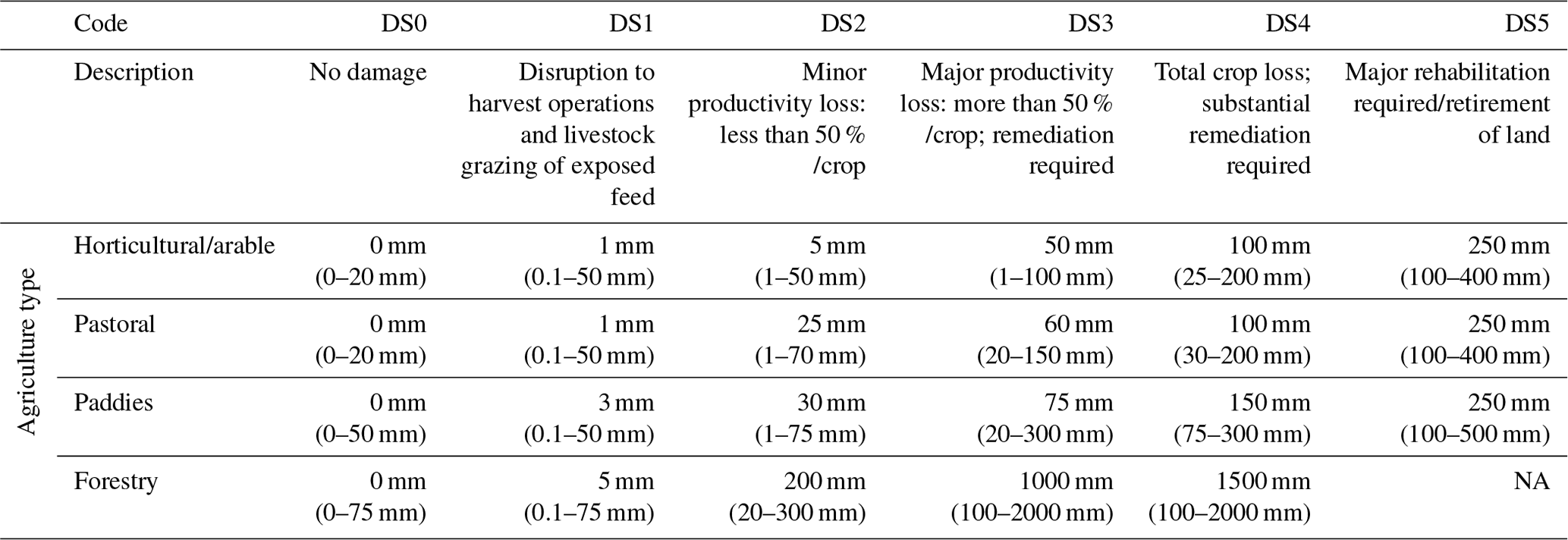

Figure 1Overview map of the study area. (a) Isopach (cm) from Dominguez and Baumann (personal communication) showing lines of equal thickness of the fallout deposit for the month of June 2011. Locations are those mentioned in Elissondo et al. (2016) as being affected by tephra fall. Background is © Google Maps 2022. Roads, locations and borders are from © OpenStreetMap contributors 2021. Distributed under the Open Data Commons Open Database License (ODbL) v1.0. (b) Mean yearly precipitation (mm) for the period 2006–2011 inferred from ERA5. Note that these values differ from those presented in the text and in Elissondo et al. (2016) as ERA5 values represent averages over a model grid cell and time step. Background is the Köppen–Geiger climate classification of Beck et al. (2018). BWk – arid, desert, cold arid; BSk – arid, steppe, cold arid; Cfb – warm temperate, fully humid, warm summer; Cfc – warm temperate, fully humid, cool summer; Csb – warm temperate, summer dry, warm summer; Csc – warm temperate, summer dry, cool summer; Dsb – snow, summer dry, warm summer; Dsc – snow, summer dry, cool summer; ET – polar, polar tundra. (c) Land cover classes from the CGLS–LC1000 dataset (Buchhorn et al., 2020). (d) Dominant soil types in the study area from the SoilGrids dataset (Hengl et al., 2017) based on the USDA soil taxonomy. All maps are projected using EPSG:32719.
2.1 Impact of volcanic hazards on vegetation
Explosive volcanic eruptions produce tephra, a generic term for pyroclasts originating from the fragmentation of parent magma, the fraction <2 mm diameter of which is referred to as ash. For sufficiently large eruptions, tephra deposits can alter the hydrology, vegetation cover and soil properties of entire regions, contributing to the perturbation of their ecosystems for months to years (Major et al., 2016; Pierson et al., 2013; Zobel et al., 2022). Direct negative impacts on and the ability of vegetation to recover from eruptions depend on complex interactions between biotic and abiotic parameters (Ayris and Delmelle, 2012; Arnalds, 2013). Biotic parameters include the type and composition of the vegetation, the biological legacy related to previous stresses and the phenological state of the plant at the time of eruption (Jenkins et al., 2014; Ligot et al., 2022). Abiotic parameters include climate (e.g. rainfall and temperature) and environmental setting (e.g. elevation, slope, orientation) (Crisafulli et al., 2015; Dale et al., 2005). For crops, impacts also depend on access to technology and mitigation measures (Magill et al., 2013; Wilson et al., 2013). Mechanisms of adverse effects of tephra on vegetation are various, including smothering and burial, breaking and abrasion, reduced photosynthesis, salt-induced stress, and limitation of pollination (Arnalds, 2013; Ayris and Delmelle, 2012; Blake et al., 2015). Critical hazard impact metrics therefore depend on the characteristics of the eruption (e.g., magnitude, intensity and style) and the properties of the deposit (i.e., thickness, grain-size distribution, content in water-soluble elements) (Cronin et al., 2014; Stewart et al., 2016).
2.2 Case study: the Cordón Caulle 2011 eruption
On 4 June 2011, a subplinian rhyolitic eruption started at Cordón Caulle volcano (CC; 40.525∘ S, 72.16∘ W; Fig. 1), part of the Puyehue–Cordón Caulle volcanic complex. The eruption began with a 24–30 h long paroxysmal phase that gradually transitioned to low-intensity tephra emissions lasting for several months (Pistolesi et al., 2015). Reported plume heights ranged from 9–12 km a.s.l. for the first 3–4 d, 4–9 km a.s.l. for the following week and <4 km a.s.l. after 14 June (Bonadonna et al., 2015; Collini et al., 2013). During the first week, westerly winds dispersed ∼1 km3 of tephra towards Argentina. Published isopach maps describe the deposit thickness associated with various phases of the eruption (e.g. Bonadonna et al., 2015; Collini et al., 2013). An unpublished report by Dominguez and Baumann (personal communication), combining data from Bonadonna et al. (2015) and Pistolesi et al. (2015), shows the spatial distribution of total deposit thickness for 4–30 June 2011 (Fig. 1a). The deposit showed low to very low concentrations of water-soluble elements potentially harmful to plant leaves (e.g., fluorine sulfur; Stewart et al., 2016).
The deposit of the CC 2011 eruption impacted three different biogeographical regions: from west to east, southern Andes and Andean foothills and lowlands (Elissondo et al., 2016). These roughly correspond to the warm temperate – fully humid, warm temperate – summer dry and arid climate classifications (Fig. 1; Beck et al., 2018), respectively, each characterized by specific assemblages of vegetation (Easdale and Bruzzone, 2018; Enriquez et al., 2021). The southern Andes are characterized by a high elevation (mean of 2000 m a.s.l.), Valdivian temperate forest and annual precipitation of 800–2500 mm, mainly occurring in June–August (Elissondo et al., 2016). Andean foothills are characterized by a gradient of annual precipitation decreasing from 800 in the west to 300 mm in the east and a vegetation of grasses, shrubs, and wet meadows covering 5 %–10 % of the area (Easdale and Bruzzone, 2018; Elissondo et al., 2016). The lowland is characterized by a cold and semi-arid climate with annual precipitation of ≤300 mm. During the 6 years prior to the eruption, this region experienced <160 mm of precipitation per year, which caused regional drought conditions. Due to water availability, the rainfall gradient strongly controls the type of farming, with pastoral farming and agriculture in Andean regions and low-intensity goat and sheep farming in the arid lowlands (Stewart et al., 2016). In addition, regions with low precipitation experience wind erosion and remobilization of loose tephra (Dominguez et al., 2020b; Forte et al., 2017; Wilson et al., 2011a, b).
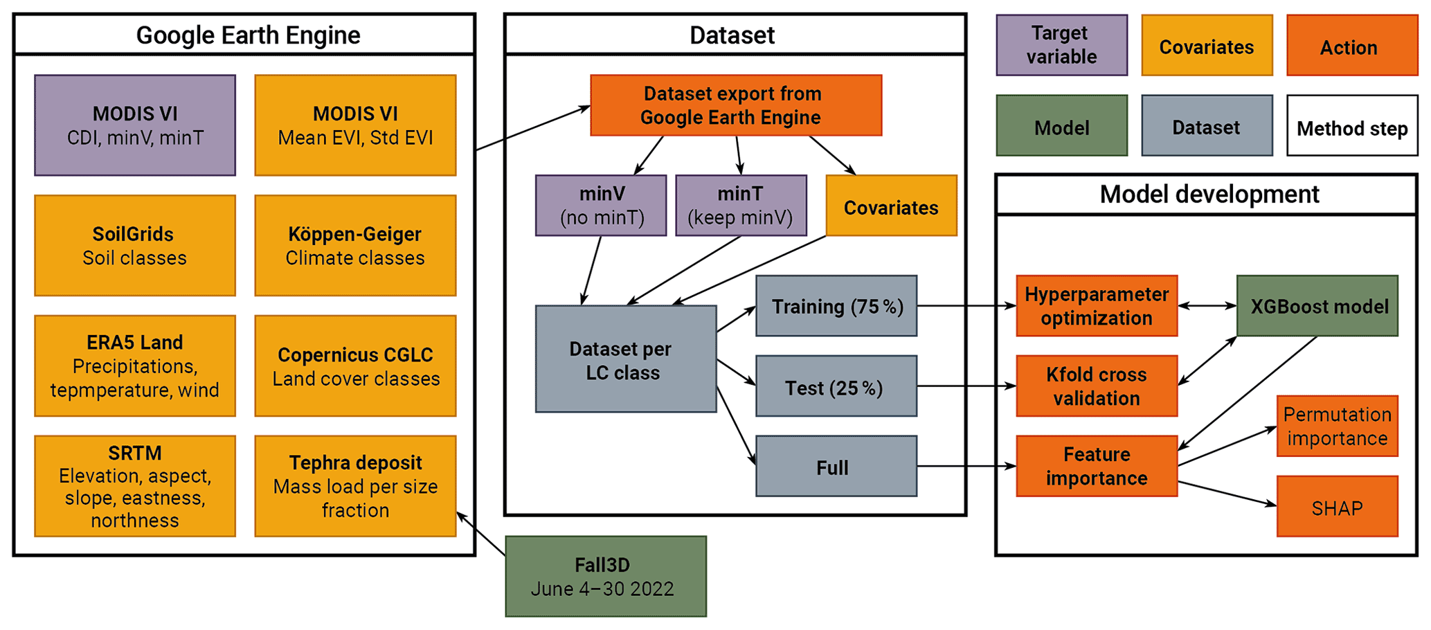
Figure 2Graphical summary of the model development. Flowchart made with https://www.diagrams.net (last access: 3 August 2022).
Figure 2 summarizes the conceptual steps of our methodology. The aim is to capture vegetation impact from multi-spectral satellite images and train a ML model to explain it as a function of covariates describing hazard and vulnerability. We detail the successive steps of this methodology, from the quantification of vegetation impact (Sect. 3.1) and covariates (Sect. 3.2) to the development, application and interpretation of the ML model (Sect. 3.3). Throughout the paper, we refer to metrics of vegetation impact as the target variable, whereas feature is used as a synonym for covariate and/or explanatory variable, and instance is used as a synonym for a geographic point.
3.1 Quantifying vegetation impact from remote sensing data
In situ assessment of vegetation (including crops) impact is typically quantified using various metrics defined depending on the purpose (e.g., percentage of destroyed vegetation or yield loss; Table 1). We use the enhanced vegetation index (EVI; Huete et al., 2002) as a remote-sensing-based proxy for biomass production (Poortinga et al., 2018; Kong et al., 2019) and consider impact as a negative deviation of the post-eruption EVI signal. The EVI is retrieved from MODIS imagery (i.e., the MYD13Q1 and MOD13Q1 V6 products) generated every 16 d at a spatial resolution of 250 m. This MODIS image collection was processed on GEE.
3.1.1 Temporal smoothing
The MODIS EVI image collection is temporally smoothed using the median pixel value over consecutive time steps (represented by the j index in Eq. 1). We test here two time windows of 1 and 3 months using the eruption date as a reference point. This approach to temporal smoothing, used to reduce artefacts, was selected over filtering-based (e.g., Savitzky–Golay filters) or non-parametric statistical (e.g., double logistic function) methods for two main reasons. Firstly, these methods are sensitive to the density and the signal-to-noise ratio of the time series (Cai et al., 2017; Li et al., 2021). As volcanoes are vast topographic edifices, frequent clouds in their vicinity make the application of such algorithms unstable and unreliable. Secondly, we focus on the impacts occurring at a medium term rather than in the immediate aftermath of an eruption, where a vegetation index (VI) can capture signals that do not record impact (e.g., increase in soil brightness due to tephra deposit). As a result, the median value over a given time window presents the most stable and conservative smoothing method around volcanoes.
3.1.2 Anomaly quantification
Multiple approaches have been developed to quantify VI anomalies for purposes ranging from early warning (e.g. Asoka and Mishra, 2015; Meroni et al., 2019; Rembold et al., 2019) to index-based parametric insurance (e.g. Martín-Sotoca et al., 2019). VI anomalies have also been used to monitor vegetation recovery after natural hazards (e.g. fires, Bright et al., 2019; volcanic ashfall, De Schutter et al., 2015), cropping intensities (e.g. Liu et al., 2020), long-term land degradation (Gonzalez-Roglich et al., 2019) or changes in vegetation dynamics (Kalisa et al., 2019). We adapt the approach of Poortinga et al. (2018) as a proxy for impact of volcanic ash on vegetation, hereafter named the cumulative difference index (CDI). The CDI is computed as
where CDIi,t is the CDI value for pixel i for consecutive j values after the eruption up to time t, is the median VI value for pixel i at a post-eruption period j in year k, Nt is a set of post-eruption periods that includes all j, k indices up to a time t, and is the long-term VI mean over the baseline (averaged over 5 years prior to eruption for pixel i and period j). VI is the vegetation index (here, EVI), and j is an arbitrary time window, referring to a subset of a year. Here, j considers a 1–3-month period, and the baseline considers 5 years of pre-eruption conditions. For the 2011 eruption of CC, the first CDI value (i.e., j=1, k=1, t=1) is simply the difference between the median VI value for April–June 2011 and the average of all April–June VI values in the period 2006–2010. The second CDI value would sum the differences over the set N2 (i.e., , k=1, t=2).
Whilst most remote sensing indices rely on ratios of pre/post conditions to define a relative anomaly (e.g., Hope et al., 2012; see Sect. 3.2.2), the CDI relies on an absolute difference. It is important to note that therefore, by definition, pixels with high EVI values will result in larger CDI changes. However, the temporal evolution of the CDI offers a new approach to capture impact and recovery. Figure 3 illustrates idealized profiles that the CDI can adopt through time. Following Eq. (1), a scenario where the CDI gradient remains negative implies that post-eruption conditions are persistently lower than the baseline (i.e., P1 in Fig. 3). A CDI flattening and reaching a zero gradient indicates a return to pre-eruption conditions (P2 in Fig. 3). If the gradient of the CDI slope becomes positive after the inflection point, the post-eruption biomass production has exceeded pre-eruption conditions. If the CDI curve flattens at a negative CDI value, the total loss in biomass due to the eruption has been partly compensated for by a temporary increase (P3 in Fig. 3). Should the absolute CDI value become positive, the total biomass loss caused by the eruption has been either compensated for or exceeded by the gains (P4 in Fig. 3). The purpose of the model is to explore conditions explaining the magnitude of impact (i.e., minV in Fig. 3) and the duration to reach it (i.e., minT in Fig. 3). The shape of the CDI curve after reaching minV is not considered here, and minV for the case of P1 in Fig. 3 is the minimum value reached after 5 years post-eruption.
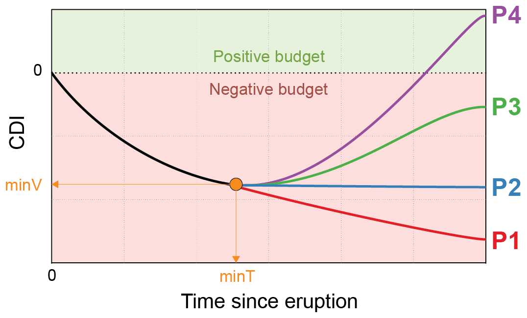
Figure 3Illustration of various possible CDI profiles through time. The x axis represents t in Eq. (1). minV represents the minimum CDI value reached by a CDI profile and minT the duration after which minV has been reached. P1 represents a scenario with a permanent degradation of the EVI. P2 represents a scenario where post-eruption conditions have returned and remain equal to pre-eruption conditions. P3 represents a scenario where post-eruption conditions have returned and temporarily exceeded pre-eruption conditions without compensating for the deficit caused by the eruption. P4 is similar to P3, but with post-eruption conditions sufficiently persisting to compensate for and exceed the deficit caused by the eruption.
Table 2Summary of variables used in the model.
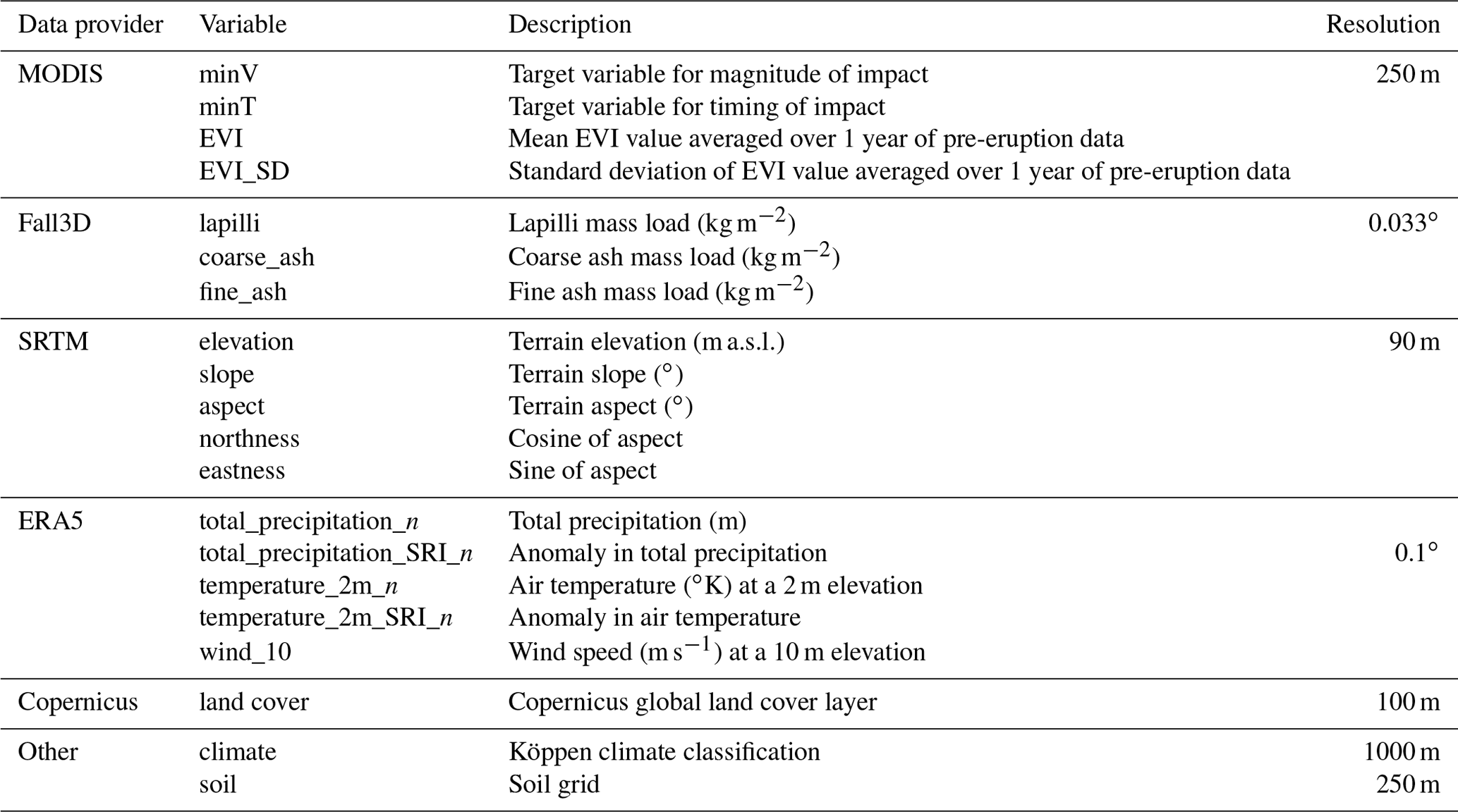
The total_precipitation and temperature_2m variables are calculated for n=1, 2, 3, 6 and 12 months.
3.2 Model features
Covariates used in the model to predict the impact (Table 2) were chosen to capture the relevant hazard and vulnerability parameters identified from the literature (Sect. 2.1). Most datasets are natively available on GEE, and others have been manually uploaded as assets. Note that the original covariate dataset contained ∼300 features. Here we present the final set of variables identified based on (i) a minimum degree of multicollinearity assessed during the exploratory data analysis phase and (ii) iterations of the process of model optimization and computation of feature importance described in Sect. 3.4.3 that allowed identifying and retaining the most informative variables.
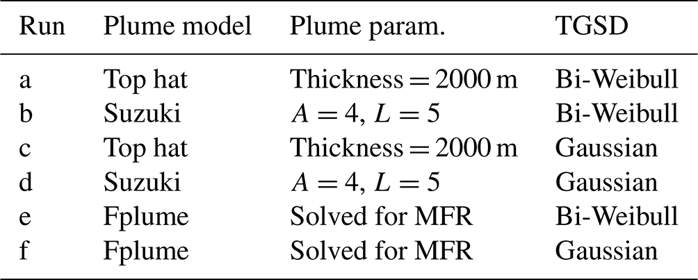
Table 3Initial parameters to the Fall3D runs. For the Suzuki plume model, A and λ are the shape factor controlling the mass distribution described by Pfeiffer et al. (2005), where λ=2 results in more mass distributed in the lower portion of the plume. The FPlume approach (Folch et al., 2016) was solved for mass flow rate (MFR, Degruyter and Bonadonna, 2012). Two total grain-size distributions (TGSDs) were tested including a field-based Gaussian (Md Φ and σΦ of 1.7 and 3.1, respectively; Bonadonna et al., 2015) and a model-based Bi-Weibull (modes at −3.13 and 4.69 Φ with respective shape factors of 0.73 and 1.1 Φ and a mixing factor of 0.64; Costa et al., 2016; Folch et al., 2020) distributions.
3.2.1 Deposit properties
Deposit thickness and grain-size distribution are the two of the main physical aspects controlling the direct impact of ashfall on vegetation (Jenkins et al., 2015). Since available isopach maps represent only deposit thickness, we reconstructed the grain-size distribution of the deposit associated with the 4–30 June 2011 phase of the CC2011 eruption using Fall3D v8.0.1 (Folch et al., 2020). The model was initialized using hourly atmospheric conditions retrieved from the European Centre for Medium-Range Weather Forecasts (ECMWF) ERA5 dataset (Hersbach et al., 2020) and daily mean plume heights reported by Collini et al. (2013). We tested several modelling schemes (Table 3) and compared the outputs against the isopach in Fig. 1a. For this, isopachs were interpolated using a generalized additive model and converted to maps of tephra accumulation using a constant deposit density. We tested densities of 1000, 2000 and 2200 kg m−2 to provide a range of tephra thicknesses for each point. The Fall3D NetCDF output was converted to a multiband GeoTIFF with each band containing mass loads for different size fractions. Size fractions computed by Fall3D were grouped into lapilli (2–64 mm), coarse ash (1–0.25 mm) and fine ash (<0.25 mm). The GeoTIFF was uploaded as an asset to GEE.
3.2.2 Climate
Atmospheric data were obtained from GEE using the ERA5 Land monthly averaged climate dataset (Hersbach et al., 2020), which provides a global reanalysis of climate variables since 1981 at a spatial resolution of 0.1×0.1∘. As the nature of the adopted ML model does not allow for using time series as covariates (see Sect. 3.4), we instead retrieve the total precipitation and the surface air temperature and compute their mean over 1, 2, 3, 6 and 12 months before the eruption. Each variable is considered both as raw values and anomalies computed as the stand regeneration index (SRI; Hope et al., 2012). As for CDI, we used a 5 years pre-eruption baseline and normalized the closest pre-eruption value by the mean value over the same period in the baseline Vi,j:
For instance, a 3-month precipitation anomaly <1 suggests that the trimester before the eruption was characterized by relatively lower rainfall compared to the same period of the year in the 5-year baseline. By considering both raw values and anomalies, we explore the relevance of each variable and potential pre-existing climatic stresses whilst also investigating what time windows are relevant for vegetation impact. The model also includes the wind velocity at the time of the eruption from the ERA5 Land dataset.
In addition to atmospheric variables, the model includes the updated 1 km version of the Köppen–Geiger climate classification by Beck et al. (2018). The study area spans three of the five main categories (arid, warm temperate and polar), with two sub-types of arid (i.e. desert – hot arid and steppe – hot arid) and four sub-types of warm temperate (fully humid – warm summer, fully humid – cold summer, summer dry – warm summer, summer dry – cool summer).
3.2.3 Terrain
Terrain data were obtained from the Shuttle Radar Topography Mission (SRTM; Farr et al., 2007) using the NASA's SRTM V3 product at a resolution of ∼30 m. Elevation, slope, aspect, eastness and northness (sine and cosine of aspect, respectively) were retrieved from GEE and used as features.
3.2.4 Land cover
Land cover was obtained from Copernicus Global Land Service (CGLS) dynamic land cover map (CGLS-LC1000, Buchhorn et al., 2020), available on GEE at a spatial resolution of 100 m yearly from 2015–2019. The land cover type is retrieved from the discrete_classification band for the closest year to the eruption (here 2015, acknowledging that the 2015 dataset possibly includes a long-term change in land cover caused by the 2011 eruption). To test the impact of tephra on various types of vegetation, we extracted the cultivated and managed vegetation/agriculture class as a proxy for cropland and the shrubs, sparse and herbaceous vegetation classes (i.e., values 40, 20, 60 and 30, respectively). In addition, we extracted a composite forest class comprising all classes tagged with forest. In the study area, present forest classes include evergreen broad leaf, both closed (112) and open (122); deciduous broad leaf, both closed (114) and open (124); and closed forest, mixed (115) and forest, not matching any of the other definitions (116 and 126).
3.3 Point sampling
In the study area, the vegetated land cover classes defined above account for 96 % of the total land cover, with the classes shrubs (38 %), sparse (26 %) and herbaceous (17 %) dominating the total count. The forest class (17 %) dominates the Andean part of the study area, whereas crops represent about 1 % of the region. A total of 5000 instances were randomly sampled for each land cover class. The target variables and covariates for all points were downloaded from GEE and stored as a GeoPandas dataframe in Python.
3.4 Setting up the machine learning model
We developed an interpretable ML model able to process big EO data to identify the most important variables and how they interact to cause the impact on vegetation. This amounts to a (supervised learning) regression task; the EO data, for training and testing, include the environmental, atmospheric, and geophysical features described above, as well as the target variables consisting in the impact metrics. The main objective is to investigate and describe the nature of the processes; performing out-of-sample predictions (i.e., model generalization) is outside of the scope of this paper. This section introduces the ML algorithm, its optimization and its interpretation processes. All computations are performed using Python 3.9 on the Gekko cluster of NTU's Asian School of the Environment, both using CPUs and GPUs.
3.4.1 ML algorithm
The main modelling challenge is to approximate complex functions mapping both minV and minT to the various investigated features. Decision trees and related methods form a general class of models suitable for such regression tasks. We opt for gradient-boosted trees, a category of decision trees that use an ensemble of so-called weak learners built sequentially to improve prediction accuracy (Müller and Guido, 2015) and capable of handling multicollinearity (Chen et al., 2022). Gradient-boosted trees have successfully been applied on EO problems (e.g., Hengl et al., 2017). Here, we used the XGBoost v.1.4.2 library, which provides an optimized and distributed implementation of gradient-boosted trees (Chen and Guestrin, 2016).
3.4.2 Hyperparameter optimization
Gradient-boosted trees rely on a range of hyperparameters governing the model's bias-variance trade-off. Selected hyperparameters (Sect. 4.4.1) were tuned by minimizing the out-of-sample mean absolute error (MAE) computed through a 5-fold cross-validation scheme using scikit-learn's RepeatedKFold and 10 000 trees. We used the Optuna library (Akiba et al., 2019) optimized on a single GPU.
3.4.3 Model interpretation
Gradient-boosted trees can accommodate non-linear effects and interactions but, as for many modern ML algorithms, come at the cost of limited interpretability. Model-agnostic interpretation methods shedding light on black-box models are actively being developed and, when applied on big EO data, provide a novel framework to identify and constrain the processes driving changes through time in Earth sciences (Batunacun et al., 2021; He et al., 2020; Sulova and Arsanjani, 2021). Amongst these, the Shapley additive explanations (SHAP) method of Lundberg et al., (2020), based on Shapley values (Shapley, 1956) and coalitional game theory, decomposes any prediction from a given model as a sum of the individual effects from each variable (Molnar, 2021). The method computes SHAP values, which quantify how a given feature act to change a model's mean prediction. We use here SHAP values to identify drivers of vegetation vulnerability in two ways. Firstly, the mean absolute SHAP value of a variable across all instances indicates a relative importance amongst all features. Secondly, individual SHAP values for a given feature and all instances provide insights into how a feature's value influences predictions. As this study does not attempt to perform out-of-sample predictions, SHAP values are computed on the full dataset. We use the TreeExplainer method of the SHAP library (Lundberg et al., 2020) to explain XGBoost's prediction.
Unlike SHAP values, permutation feature importance ranks features based on their direct impact on model performance (Breiman, 2001; Fisher et al., 2019). We use it as a complementary approach to SHAP values. Permutation importance is also computed on the full dataset using scikit-learn's permutation_importance function using 10 permutations of each variable and computing the change in the coefficient of determination R2.
3.4.4 Modelling scheme
A model is trained separately for each land cover class defined in Sect. 3.3, with one additional model trained on all land cover classes jointly and using the land cover class as a feature. Since XGBoost does not support multi-output regressions, each dataset is used as an input for two models trained using either minV or minT as a target variable (Fig. 3). To include some dependence between the two impact metrics, the model predicting minV is trained with minT removed from the features, whereas the model predicting minT is trained with minV in the list of features.
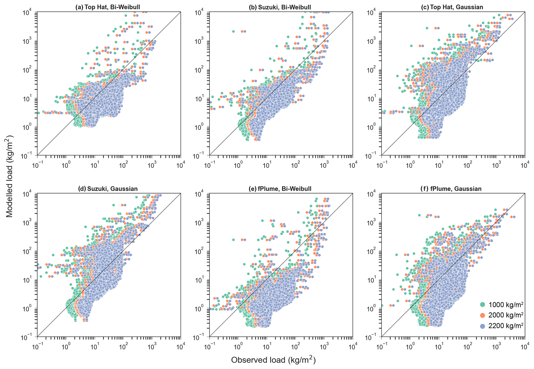
Figure 4Relationship between the tephra accumulation modelled with Fall3D and inferred from isopach for the various modelling schemes (Table 3). Colours consider various densities used to convert deposit thickness to mass loads. Panels follow Table 3. The black line shows a hypothetical 1:1 relationship.
4.1 Deposit reconstruction
To select the best Fall3D run shown in Table 3, 10 000 points were randomly sampled in space and used to retrieve both the modelled tephra load and the thickness obtained from interpolated isopach (Fig. 4). Although all model runs are capturing the general trend, mismatches can be attributed to modelling issues (e.g., limitation in describing sedimentation from the plume margin or aggregation processes; Bagheri et al., 2016; Poulidis et al., 2021) and isopach interpolation using a bulk density. In the perspective of these limitations, we adopted run b (i.e., Suzuki plume model with a Bi-Weibull grain-size distribution; Table 3) as it generally shows a minimum spread across the 1:1 line and provides a conservative scenario (Fig. 4). Figure 5a compares the modelled load for the selected run with the isopach. The model captures both the general extend of the deposit and the various lobes generated as a function of variable wind conditions throughout the eruptive phase.
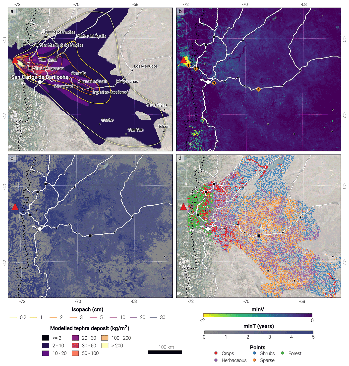
Figure 5(a) Modelled load using Fall3D run (b) (kg m−2; Table 3) overlain with isopach (cm). (b) Spatial distribution of minV. Numbered orange diamonds are referenced in the text. (c) Spatial distribution of minT. (d) Dataset of points sampled in GEE coloured by their land cover class. When not specified, legend items follow Fig. 1. Background is © Google Maps 2022.
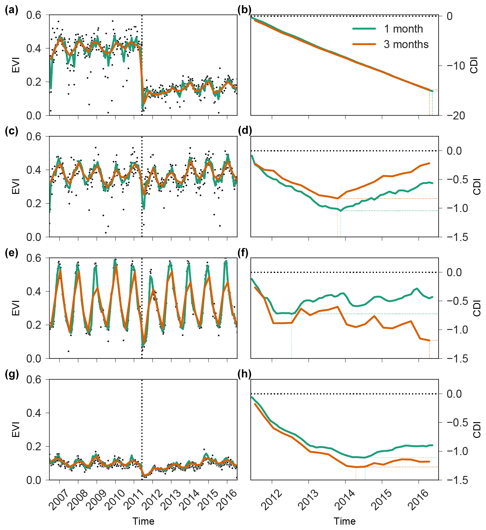
Figure 6Time series of EVI (a, c, e, g) and monthly CDI (b, d, f, h) for the four points described in Sect. 4.2 and located in Fig. 5. Black dots are raw (i.e., non-composited) MODIS data, whereas green and orange lines are composited collections using a kernel of 1 and 3 months, respectively, as described in Sect. 3.1. (a, c, e, g) The vertical black dashed line indicates eruption time. (b, d, f, h) The horizontal black dashed line indicates a neutral budget (Fig. 3). Coloured dotted lines indicate the location of minV and minT.
4.2 Anomaly quantification
Figure 6 shows an illustration of time series of EVI and associated monthly CDI for four representative points in the study area (Fig. 5b) chosen to represent the spread in tephra accumulation and vegetation/climate types and using compositing windows of 1 (green) and 3 (orange) months. Seasonal EVI patterns, with high values in the summer reflecting active growth and low values in the winter reflecting plant dormancy, indicate that the eruption occurred during a period of low growth (Elissondo et al., 2016). Point 1 (Fig. 6a, b), located 23 km southeast of the vent, is characterized by herbaceous vegetation and a modelled tephra load of 330 kg m−2 (thicknesses of 165–330 mm when converted with deposit densities of 2000 and 1000 kg m−3, respectively). The sharp drop in EVI after the eruption and the following persistent lower values compared to the pre-eruption baseline translate into a CDI profile showing a negative slope, which indicates that the system did not return to pre-eruptive conditions. This observation agrees with existing DDSs (Table 1), where accumulations ≥150 mm result in substantial vegetation destruction. Point 2, located 45 km southeast of the vent and 7 km from Villa La Angostura, consists of closed, evergreen broadleaf forest. With 40 kg m−2 of tephra accumulation (thickness of 20–40 mm for the same densities as Point 1), EVI values show a slight decrease compared to pre-eruption conditions lasting for a couple of years, after which a general trend is observed leading to larger EVI values than the baseline (Fig. 6c). This translates into CDI profiles showing a negative trend for 2 years after the eruption, after which a positive trend indicates better conditions compared to the baseline (Fig. 6d). When compared to existing DDSs for forestry (Table 1), the modelled thickness spans damage classes 0–3, ranging from no impact to minor productivity loss. Point 3 is 112 km from the vent in the vicinity of San Carlos de Bariloche. Classified as crops by the CGLS land cover and looking like pastoral grazing fields from high-resolution satellite imagery, it was affected by 7 kg m−2 of tephra (thickness of 3.5–7 mm; damage classes 0–3; Table 1). Both compositing time windows show a reduction in EVI values for at least one season after the eruption (Fig. 6e, f). Finally, Point 4 is located 240 km southeast of the vent close to Ingeniero Jacobacci and was affected by 10 kg m−2 of tephra (i.e. 5–10 mm). Classified as herbaceous vegetation in the CGLS dataset but looking like farmland with a mixture of pasture and crops on high-resolution satellite imagery, both EVI and CDI profiles indicate a return to pre-eruption conditions after ∼3 years, after which a positive CDI slope indicates temporary better conditions (Fig. 6g, h).
Figure 6 illustrates the differences in quantifying minV and minT when using time windows of 1 and 3 months in Eq. (1). A 1-month window closely follows local trends and results in irregular CDI curves, whereas a 3-month window over-smooths local variations. Although both approaches commonly result in similar results, Point 3 illustrates how the two windows can induce different interpretations. We adopt a 3-month kernel for two main reasons. Firstly, the visual comparison of the spatial distribution of minV and minT on a map shows that such differences occur locally whilst preserving the general spatial distribution. Secondly, points displayed in Fig. 6 are not heavily affected by cloud coverage, and the 1-month kernel does not reflect the typical effects that clouds can induce when using such a small compositing time window (e.g., sparse time series and artefacts). This is generally not the case, either around the Cordón Caulle volcano, where the region closer to the vent suffers too much cloud coverage to be resolved by a 1-month kernel, or around most volcanoes around the world, where large and high edifices are often cloudy. Therefore, the 3-month kernel provides a more conservative approach and enables reproducibility to other case studies.
4.3 Impact mapping
Figure 5b displays the spatial distribution of minV in the study area. The region with the minimum minV value extends up to 25 km southeast of the vent and corresponds to accumulations of ∼550 kg m−2. Although conspicuous, it is impossible to unequivocally attribute this impact to tephra fallout in proximal area where other hazards can occur (e.g., pyroclastic density currents, lahars). Except for this region, the impact within the first 80 km east of the vent is relatively limited, beyond which a sharp, north–south-oriented decrease in minV values occurs. This rapid change corresponds to a change in rainfall amount, a transition from well-developed Andosols to very weakly-developed Regosols, and a region dominated by forests to one dominated by shrubs and herbaceous vegetation (Fig. 1; Sect. 2.2). In this region, minimum minV values are , and the spatial distribution of minV reflects the spatial distribution of tephra fallout. Negative minV values extend eastwards beyond the town of Los Menucos, suggesting that impact occurred with accumulations ≤2 kg m−2. Due to the use of a 3-month kernel, minT is a discrete rather than a continuous dataset (i.e., a minT value of 4.5 months suggests that minV was reached between 3–6 months after eruption onset). The spatial distribution of minT (Fig. 5c) generally reflects minV and the pattern of tephra accumulation. Note that artefacts related to non-vegetated areas are ignored (e.g., bare rock and snow-covered mountains in the S).
Figure 5d shows the distribution of sampled points by land cover, and selected relationships are plotted in Fig. 7. Although Fig. 7 a displays a general negative relationship between minV and the tephra load, a simple linear relationship fails to accurately capture the variability of impact. For minT, Fig. 7b and c show how minT is distributed around three main modes of tephra load and minV. Land cover classes that are most impacted by long minT values are forests and herbaceous, which are the two classes the most exposed to heavy loads (Fig. 5). Plotting minT shows a distribution centred around three modes of about 400, 1000 and 1700 d (Fig. 7b). High minV and tephra loads generally result in larger minT values.
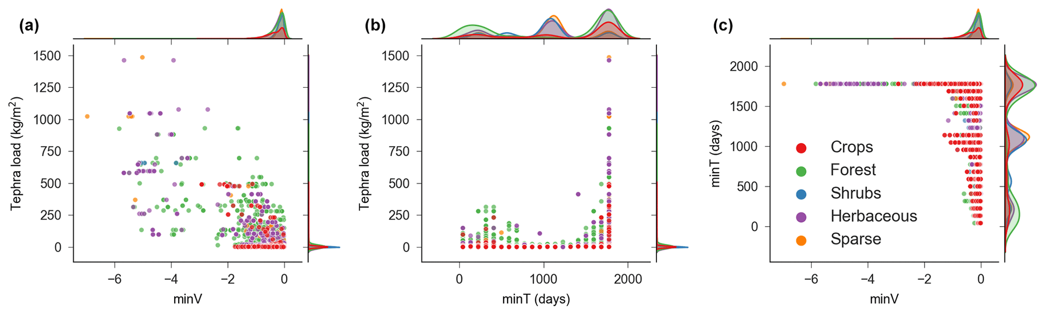
Figure 7Relationship between (a) minV and the total tephra load, (b) minT and the total tephra load, and (c) minV and minT as a function of the land cover class. The marginal axes contain a kernel density estimate of the underlying population for each land cover class. For readability all forest sub-groups are grouped.
4.4 ML model
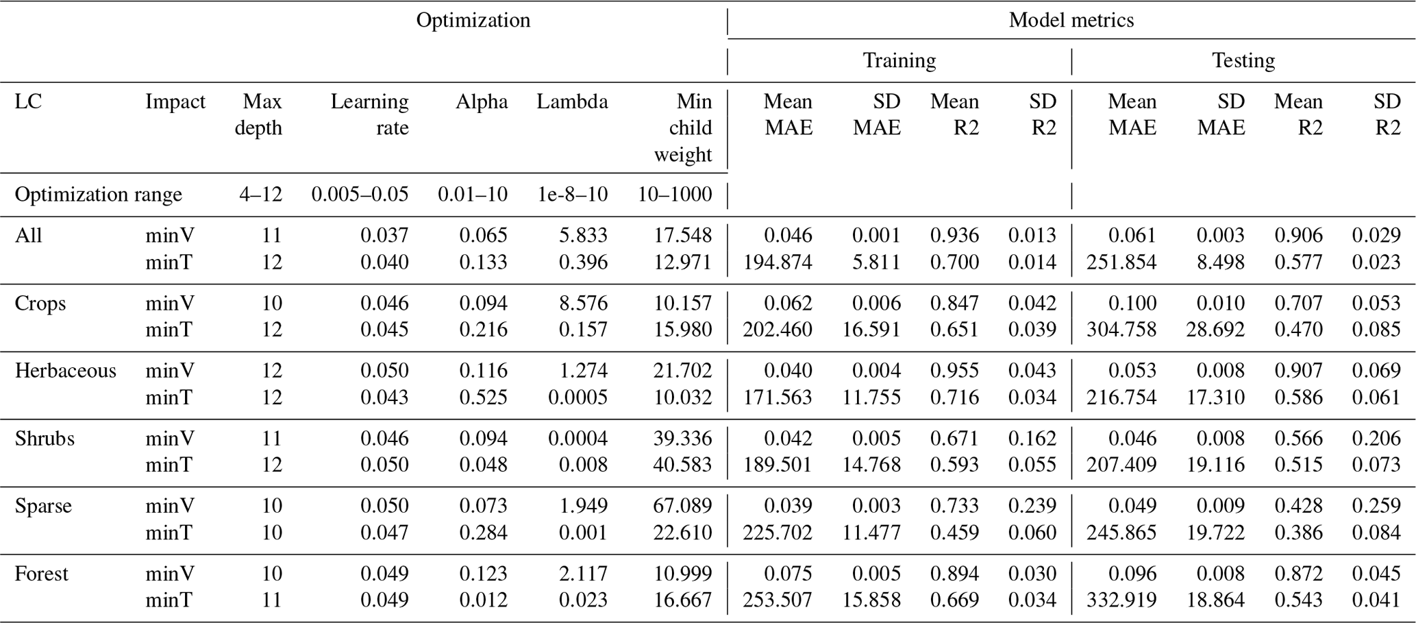
Table 4Summary of the trained models. The Optimization columns group reports the hyperparameter values obtained with the optimization process. The Model metrics columns group reports the mean absolute error (MAE) and the r2 coefficients on both training and test datasets. The mean and the standard deviation (SD) were obtained by 5-fold cross validation with three repeats.
4.4.1 Model performance
Table 4 presents the results of the optimization of hyperparameters on the dataset shown in Fig. 5d and the associated model metrics. The MAE and R2 were computed on both training and testing datasets using a cross-validation with five folds and three repeats. We compare training and testing prediction error as an indication of the degree of overfitting of the model. As expected, model metrics obtained on test datasets were lower than those using training data. Based on the R2 of the testing data and minV, models trained on all land cover classes and on herbaceous vegetation performed well (R2>0.9), followed by forests (R2>0.8) and crops (R2>0.7). The particularly low R2 value for sparse vegetation can be attributed to the presence of <10 % vegetated cover in this class, which is dominated by bare soil or rock. The R2 values of minT are consistently lower than those for minV and never exceed 0.6, which we partly attribute to its discrete nature.
Overall, the comparison of error metrics between testing and training sets reveals that models trained on the various datasets have various degrees of generalization ability, with the caveat that the validity of the insights provided by the different models should be considered in the perspective of their respective performances. The broadest dataset considering all land cover classes and minV results in high training (0.94) and testing (0.91) R2 values. We use this good performance and similarity between both values as an indication that the model is likely not overfitting and yields good generalization.
Table 5Ranking of feature importance for minV computed using mean absolute SHAP values and permutation importance for all land cover classes. For each column, the 10 most important features are in bold. Variable names follow Table 2. Herb. stands for herbaceous.
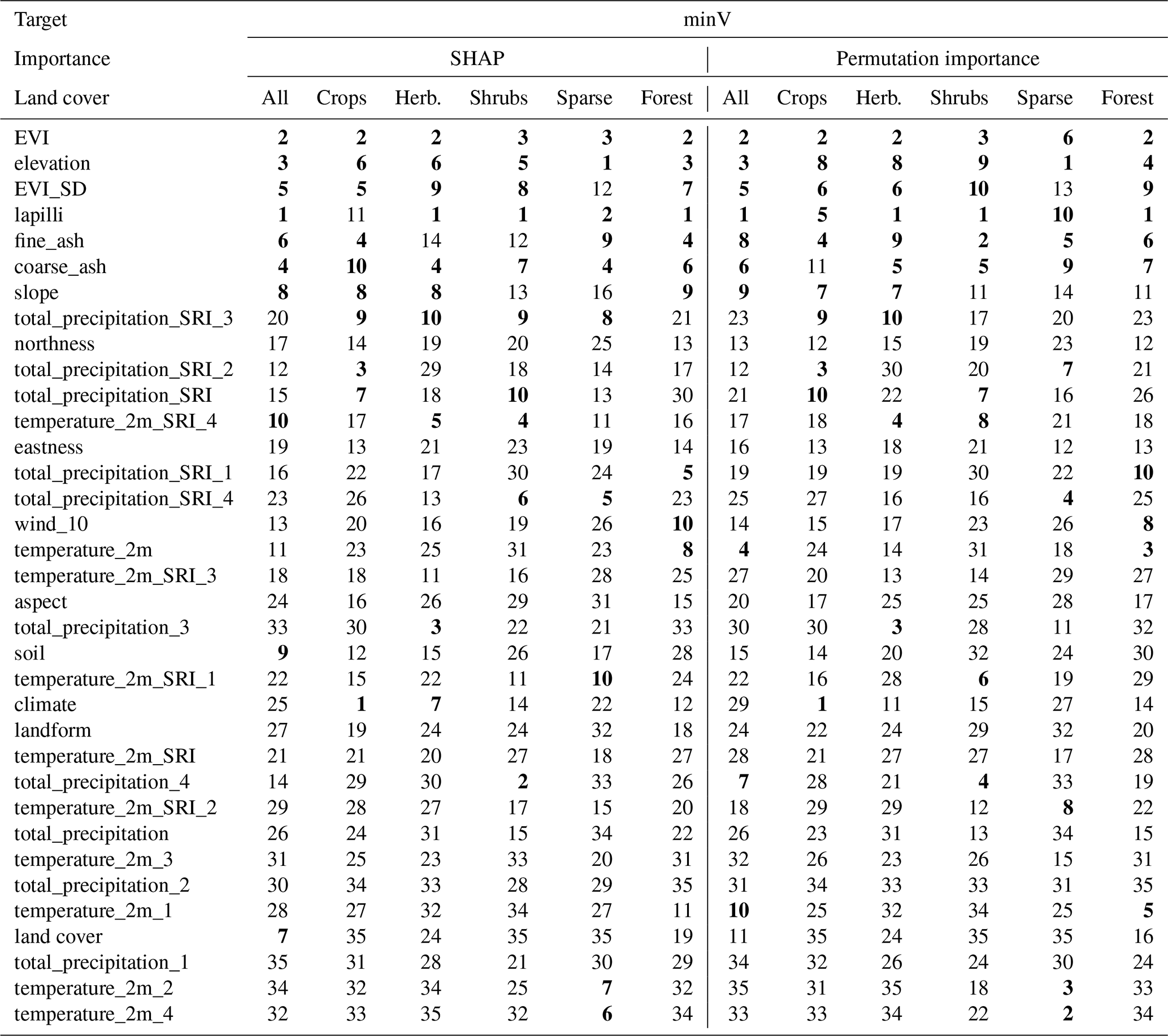
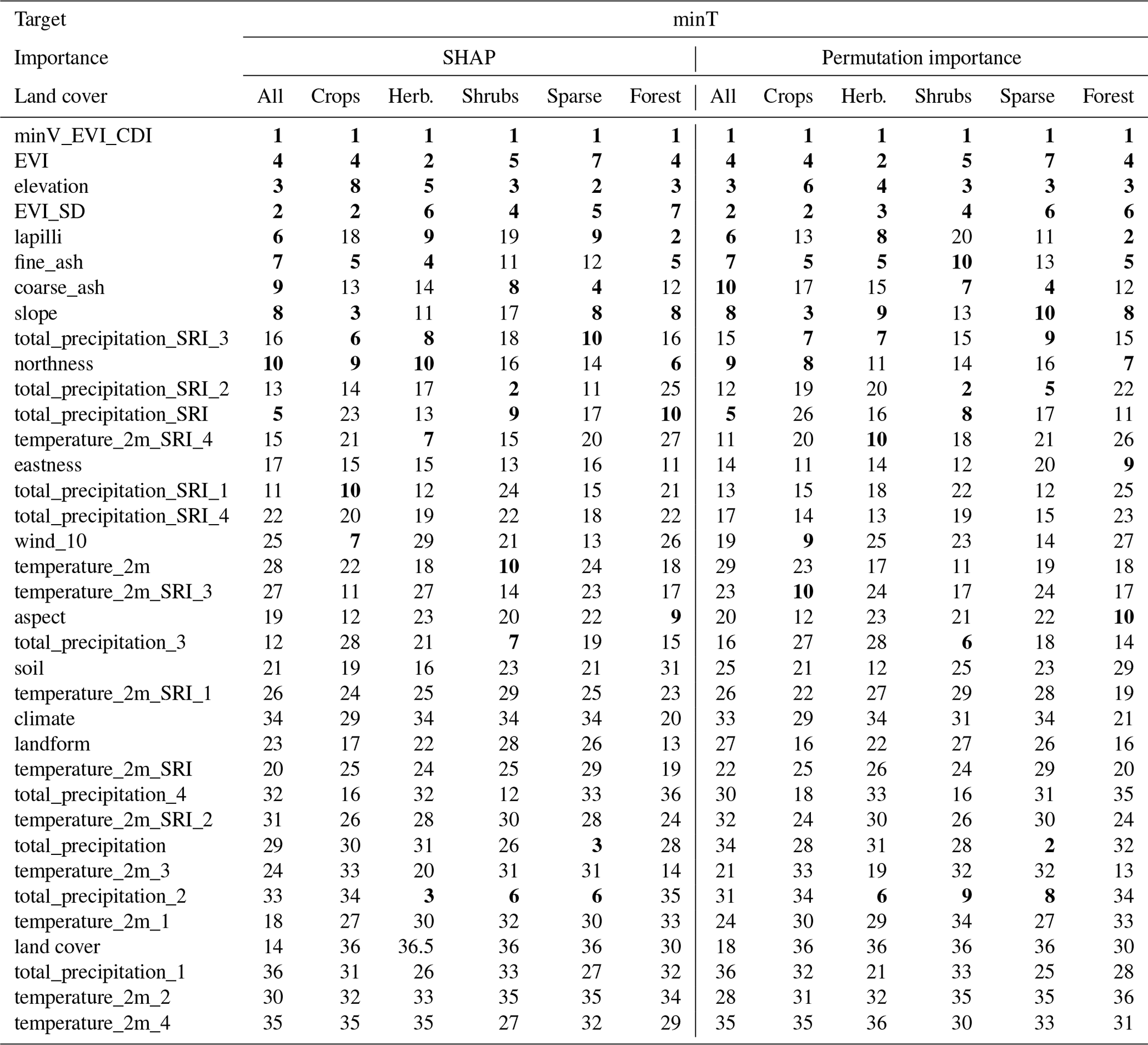
Table 6Ranking of feature importance for minT computed using mean absolute SHAP values and permutation importance for all land cover classes. For each column, the 10 most important features are in bold. Variable names follow Table 2. Herb. stands for herbaceous.
4.4.2 Feature importance
Tables 5 and 6 summarize feature importance for each land cover class using the mean absolute SHAP value and permutation importance. Although some differences exist, both methods yield similar results, thus implying that features that contribute the most to predictions (SHAP importance) also improve the model's generalization error (permutation importance). Unless specified, this section focuses on SHAP importance.
EVI and elevation are the two features that consistently rank in the top 10 of the most important variables across impact and land cover. For minT, minV is the most important variable, which suggests that both impact metrics are dependent. EVI ranks especially high, which indicates that the mean EVI value computed over the year before the eruption provides an important background level to the model. This result is a consequence of the cumulative sum of absolute differences behind the CDI, which implies that pixels with higher EVI values are prone to larger CDI impacts (Sect. 3.1.2). The variable lapilli is the most important for minV for all land cover classes but crops (SHAP value) and sparse (permutation importance) and ranks high when predicting minT for all and the forest land cover classes.
For forests, minV is best predicted, in decreasing order, by lapilli, EVI and elevation, which are respectively a deposit, a proxy for a biotic and an abiotic parameter. Note that using permutation importance instead of SHAP importance suggests that the third most important variable is surface temperature, which is correlated to elevation. In parallel, minT is driven by minV, lapilli, elevation and EVI, which indicates that the duration of impact is dominantly proportional to the magnitude of impact and the tephra load. In comparison, the minV of herbaceous vegetation is controlled by lapilli, EVI and the 6-month precipitation, which indicates the same hierarchy of importance of deposit, biotic and abiotic parameters as for forests, whereas minT is controlled by minV, EVI, the 3-month precipitation and fine ash. Interestingly, this suggests that impact duration does not primarily depend on any deposit variable, the most important of which (i.e., fine ash) is different to the parameter controlling the magnitude of impact (i.e., lapilli). As a final example, no deposit property ranks in the top three variables controlling the minV values of crops, which include climate, EVI and the 3-month precipitation anomaly. The first deposit parameter, fine ash, ranks fourth, which indicates that the vulnerability of crops to ash fallout is dominantly constrained by biotic and abiotic parameters. Fine ash ranks fifth for minT, which is mainly driven by minV, EVI and the slope, and illustrates how abiotic parameters can potentially dominantly control impact magnitude and duration.
4.4.3 SHAP dependence plots
SHAP dependence plots (Fig. 8) display, for each instance in the dataset (i.e., a point in Fig. 5d), the SHAP value of a given variable as a function of its actual value. For a given instance and a given variable, a negative SHAP value implies that the variable contributed to reducing the predicted value compared to the mean prediction of the model. Therefore, a negative SHAP value for minV implies a contribution to increase the magnitude of impact, whereas a negative SHAP value for minT implies a contribution to decrease the duration of impact.
Impact of deposit on minV predictions
Figure 8a is the dependence plots for lapilli. With loads ≤60 kg m−2 of lapilli, SHAP values are contained within 0±0.1 but drastically drop for larger loads. With lapilli dominantly impacting the vicinity of the volcanic source, <4 % of all instances are affected by accumulations >60 kg m−2, with those areas dominantly consisting of forests with additional vegetation classified as shrubs and herbaceous (Fig. 1c). Despite limited points, Fig. 8a suggests stepwise decreases in SHAP values for lapilli loads of ∼60, 230 and 550 kg m−2. Using a deposit density of 1000 kg m−3, thicknesses of 60, 230 and 550 mm span the D1–D4 damage states for forestry (Jenkins et al., 2014; Table 1). Using the pastoral class of Table 1 as an analogue for shrubs and herbaceous vegetation, these accumulations suggest that, for crops, substantial to major land rehabilitation is required before recovery. These observations confirm the relationships between minV, minT and the deposit load shown in Fig. 7: points affected by high lapilli loads result in minT values larger than ∼1300 d and an impact that persisted for years after the eruption. These high impact metrics explain why lapilli is the most important variable to predict minV. Lapilli is likely to cause a direct, physical impact from the high kinetic energies (e.g., Blake et al., 2015; Osman et al., 2019) and breakage from a static load and burial (Arnalds, 2013; Ayris and Delmelle, 2012), which is captured as a strong anomaly by our method and results as the most important variable. Plotting the dependence plot of lapilli for the model trained on the generic forest land cover class (Fig. 8b) indicates that the 2-month precipitation anomaly contributes to further explaining the influence on the SHAP value, with points with an anomaly <0.85 displaying lower SHAP values.
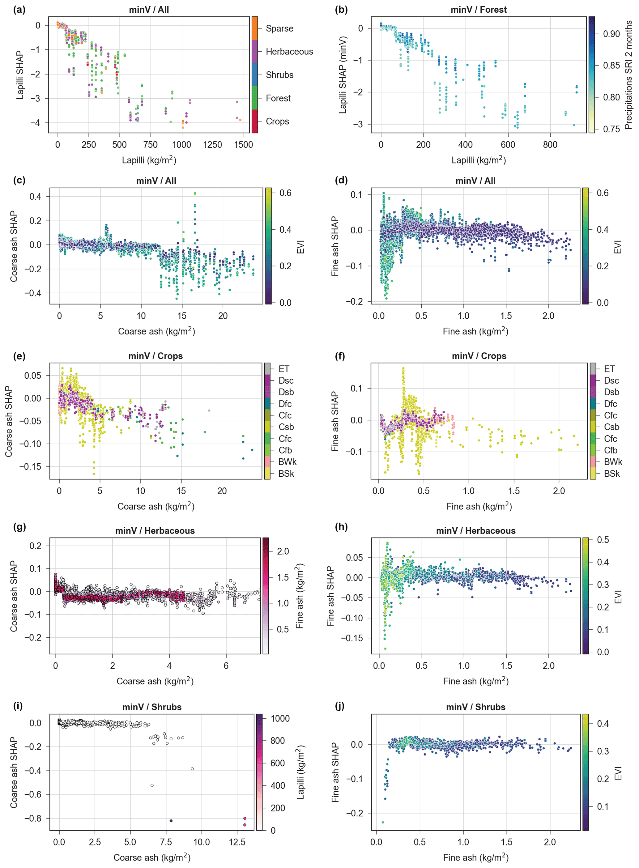
Figure 8SHAP dependence plots illustrating the effect of deposit on the minV value predicted by the models for (a) lapilli using all land cover classes, (b) lapilli on the forest subclass, and (c–j) coarse and fine ash for selected land cover classes. The hue of the points is related to additional explanatory variables. For panels (a), (e) and (f), the colour scheme follows Fig. 1. Negative SHAP values contribute to decreasing minV and therefore increase impact.
Dependence plots for coarse and fine ash (Fig. 8c, d) display similar – although less conspicuous – drops in SHAP values for accumulations of 12 and 1.7 kg m−2, respectively, with SHAP values on average 1 order of magnitude smaller than for lapilli. Considering that fine deposits are denser than coarser ones, a density range of 1000–2000 results in thicknesses of 6–12 and 0.9–1.7 mm for coarse and fine ash, respectively, which cover the D1–D3 damage classes for horticultural/arable and pastoral agriculture (Table 1). Note that these thicknesses should be regarded as minimum values as we convert here individual size fractions to total deposit thickness. Figure 8e–j also shows the effect of ash for models trained on specific land cover classes. For crops (Fig. 8e–f), coarse and fine ash are the 10th and the 4th most important variables, respectively. Coarse ash seems to induce drops in SHAP values for loads of 2, 4 and 10 kg m−2. There is clearly an effect of fine ash on SHAP values, but the oscillatory pattern is difficult to explain for loads ≤0.5 kg m−2, especially for the Csb climate class where most crops are found (i.e., warm temperate, summer dry, warm summer), and probably depends on additional variables not accounted for in the model (e.g., geographic distribution of plant-specific effects such as ash retention as a function of leaf morphology). Beyond 1 kg m−2, SHAP values are consistently negative. Coarse and fine ash are the 4th and the 14th most important variables for minV for herbaceous vegetation. The coarse ash shows more negative SHAP values when associated with fine ash. Fine ash is generally beneficial for herbaceous vegetation with low EVI values (Fig. 8h). For herbaceous vegetation, the most negative SHAP values are found for high-EVI with accumulations ≤1 kg m−2. Incidentally, such accumulations also correspond to the highest SHAP values. Since no covariate satisfactorily explains this contrasting behaviour, this is either due to a model artefact or to variables that are not accounted for in the model. For shrubs (Fig. 8i, j), coarse and fine ash are respectively the 7th and 12th most important variables. Coarse ash suggests a decrease in SHAP values for loads of ∼6 kg m−2, beyond which the magnitude of the negative effect increases with the lapilli load. Fine ash does not show any trend or sharp break.

Figure 9(a–e) SHAP dependence plots illustrating the effect of various variables on the prediction of minV. (a–b) Effect of EVI (a) and elevation (b) on the SHAP value as a function of the coarse ash load. (c) Violin plot showing the distribution of SHAP values for each land cover class with a box-and-whisker plot overlain. (d) Effect of wind speed on the SHAP values as a function of climate. (e) Effect of the 3-month precipitation anomaly on the SHAP value as a function of land cover. (f) Spatial distribution of 3-month precipitation anomaly SHAP values. Map tiles by Stamen Design CC BY 3.0; map data © OpenStreetMap contributors.
Impact of other features on the prediction of minV
Figure 9 shows SHAP dependence plots for variables other than the deposit. Figure 9a confirms the importance of EVI on minV, where all points with EVI <0.1 result in positive SHAP values and all points with EVI >0.3 result in negative SHAP values. This observation is partly a consequence of the use of Eq. (1), where the value of is generally larger for higher EVI values. Figure 9a also suggest a dependence of this relationship on the load of coarse ash, which slightly increases SHAP values for low EVI but decreases them for higher values. Elevation is the third most important feature for predicting minV and shows a breakpoint at an altitude of ∼1000 m a.s.l. (Fig. 9b), below which SHAP values are dominantly negative. Above this elevation, SHAP values are generally positive, regardless of the intensity of ash accumulation. Land cover, the seventh most important feature, indicates that crops dominantly contribute to increasing impact in the model (Fig. 9c). Sparse vegetation also has a negative but less pronounced effect on SHAP values, whereas shrubs and herbaceous vegetations have a neutral effect. The SHAP values of forests tend to reduce the impact, which corroborates the higher resilience of trees to tephra fallout (Table 1).
Wind and precipitation partly control the residence time of ash on leaves and therefore the impact (Ayris and Delmelle, 2012). Although variables used here only consider pre-eruption atmospheric conditions, they are indirectly used as indicators for post-eruption patterns. The impact of wind speeds on SHAP values suggests breakpoints at 0.2 and 1.2 m s−1. SHAP values are strongly negative below 0.2 m s−1, generally positive up to 1.2 m s−1 and generally negative above (Fig. 9d). This supports the idea that wind contributes to reducing the residence time of ash on leaves, but the aeolian remobilization of ash at higher wind speeds can negatively impact vegetation (e.g., Arnalds, 2013; Craig et al., 2016b; Elissondo et al., 2016; Wilson et al., 2011a, b). Although depending on additional parameters (e.g., surface roughness, ash properties, soil humidity, rainfall intensity), an empirical value for onset of remobilization of 0.4 m s−1 has been used in the literature and agrees with our results (e.g., Folch et al., 2014; Liu et al., 2014). Leadbetter et al. (2012) observed that ash resuspension is suppressed if precipitation rates exceed 0.01 mm h−1, and our model indicates that most negative SHAP values occur for relatively dry climates. The most important precipitation variable for predicting minV with all land cover classes is the precipitation anomaly computed over 3 months before the eruption, which mostly shows a negative anomaly (i.e., anomaly <1; Table 6; Fig. 9e). This precipitation anomaly shows a clear break at a value of 0.87, for which SHAP values are dominantly negative below and positive above. Above a value of 1, SHAP values increase. Figure 9e shows a negative peak in SHAP values between an anomaly of 0.85–0.87 across all land cover classes but stronger for crops. Plotting SHAP values on a map (Fig. 9f), the spatial clustering of negative SHAP values corresponds to the location of crops between San Carlos de Bariloche and Comallo (Fig. 1). No variable unequivocally explains this spatial clustering.
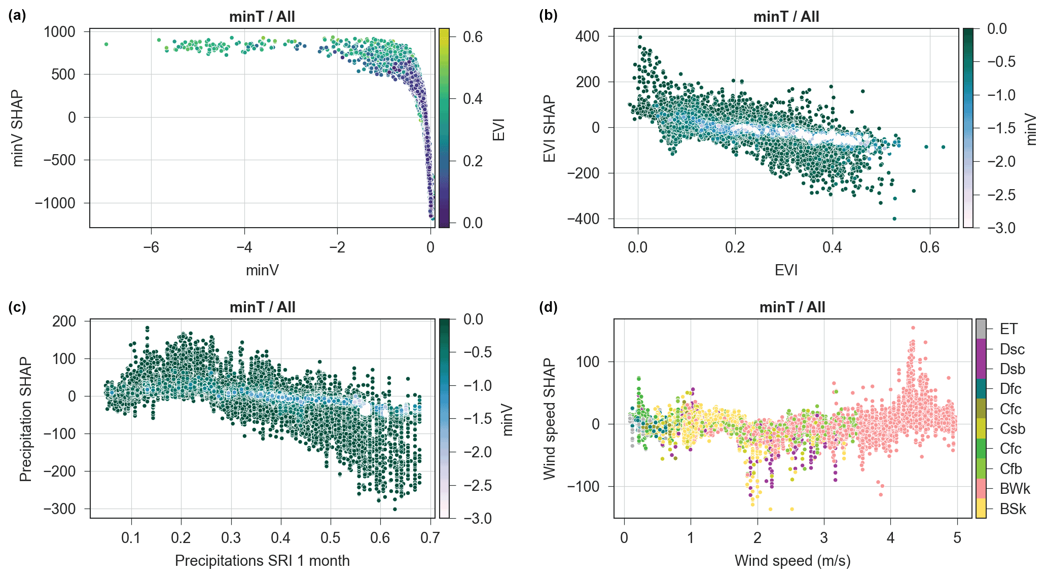
Figure 10SHAP dependence plots for minT showing the effect on the SHAP value from (a) minV as a function of EVI, (b) EVI as a function of minV, (c) 1-month precipitation anomaly as a function of minV and (d) wind speed as a function of climate. Negative SHAP values contribute to decreasing minT and therefore decrease impact the duration for reaching minV.
Features driving minT
With a mean absolute SHAP value >7 times larger than any other variable, minV is by far the most important for predicting minT (Fig. 10a), with a cut-off between positive (i.e., increasing the value of minT) and negative (i.e., decreasing minT) at a minV value of ∼0.15. The effect of EVI on minT is the opposite of minV (Fig. 9a): although high EVI values tend to increase the impact magnitude (lower minV), they generally contribute to reducing the impact duration (i.e., Fig. 10b). Interestingly, this trend disappears as minV increases. This can be explained by the fact that points affected by high minV values in Fig. 10b are associated with relatively high minT values (Figs. 7; 10a). These points are associated with damage classes suggesting land retirement, and their recovery is therefore independent of the pre-eruption EVI level. The 1-month precipitation anomaly is the fifth most important variable for minT (Fig. 10c), and SHAP values are mostly positive below an anomaly of 0.3 and mostly negative above 0.5. As for EVI, high minV values are less sensitive to the general trend. Finally, Fig. 10d shows the effect of the wind speed at the time of eruption on minT as a function of the climate. Wind speeds >4 m s−1 considerably increase minT, especially in an arid climate (i.e., BWk) where the vegetation is mostly shrubs, herbaceous and sparse. Points with positive SHAP values at wind speeds >4 m s−1 are characterized by accumulations of fine ash >0.5 kg m−2. In contrast, points with minimum SHAP values between wind speeds of 1.8–2.8 m s−1 correspond to crops close to Piedra del Aguila and show fine ash loads <0.5 kg m−2.
The proposed methodology provides a new framework to systematically assess the vulnerability of vegetation to tephra fallout as a dynamic, multi-variate problem. Its application to the CC 2011 eruption highlights how big EO datasets and interpretable machine learning could help acquire new knowledge from tens to hundreds of understudied eruptions recorded in archives of multispectral images. This approach aligns with FAO's objective of gaining a global understanding of vegetation vulnerability through the systematic study of their impacts and, in turn, contributes to various Sustainable Development Goals (SDGs 2.4, 13.1, 15.3). Specific to volcanic risk, this is the first effort to provide a large-scale, quantitative basis to estimate the impacts of explosive volcanic eruptions on food production. On a longer timescale and large spatial scale, this is the first step towards tackling the unaddressed black elephant event that is the risk of future large eruptions on food security (Lin et al., 2021).
5.1 Validation and causal inference
Our methodology attempts to highlight impact mechanisms either occurring from the direct action or arising from interactions between physical properties. Since we neglect the impact from water leachable elements (e.g., Stewart et al., 2020), the approach is more suited to dominantly magmatic events rather than eruptions with a significant hydrothermal component. Impact patterns captured by our methodology are corroborated by lessons learned from empirical post-EIAs and experiments. For CC 2011, the model suggests that, except for points subjected to destruction from large tephra loads, various biotic and abiotic variables tend to have a more critical control on both impact magnitude and impact duration than deposit properties (Tables 5 and 6). SHAP dependence plots for deposit properties (e.g., Fig. 8a–e) identify similar tephra thresholds as those in existing DDSs (Table 1). Nevertheless, numerous evidences reported in post-EIAs as well as controlled experiments outline the dependency of impact mechanisms to size distribution, ranging from physical impact for large lapilli to a reduction of light interception from fine ash leading to a decrease in photosynthesis (e.g., Ligot et al., 2022). DDSs must therefore consider other hazard impact metrics than only tephra thickness, and Figs. 8–10 are the first attempt towards this objective. The method is also able to capture impacts arising from interaction between other parameters than deposit properties. For instance, Fig. 9d suggests that the model captures the general relationship between presence of ash, precipitation (inferred from climate) and wind speed in controlling the impact from aeolian remobilization. This demonstrates the ability of the model to identify complex and dynamic processes, and cross-validating thresholds inferred from the model with values from existing post-EIAs and experiments provides a systematic framework to generalize observations made at different scales (Dominguez et al., 2020a; Forte et al., 2017; Leadbetter et al., 2012; Liu et al., 2014).
Despite these observations, methodologies for interpretable ML should be carefully used when attempting to infer causality from correlations/associations. Suggestions of causality are currently restricted to effects that rely on phenomena that have been either witnessed in the field or experiments. Other variables considered in our dataset show conspicuous and complex patterns that we are unable to explain (e.g., Figs. 8f, 9e). Such patterns have two possible explanations (or a combination of both): either (i) the model fails to accurately capture the underlying relationship between feature and target variable or (ii) the relationship is complicated by other factors (e.g., feature interactions, confounding variables), including unobserved ones. Investigating which association captures true causality therefore requires the development of synergies between various relevant disciplines (e.g., physical volcanology, ecology, soil sciences, disaster risk reduction). The development and adaptation of existing causal inference methods in Earth sciences to investigate a system's causal interdependencies is an active topic of research (Runge et al., 2019).
5.2 Towards a model for agricultural crops and food production
The methodology currently relies on the CGLS-LC100 land cover dataset to distinguish between natural vegetation and agriculture. We focus here on agricultural crops which, despite representing ∼1 % of the study area, show the highest vulnerability to tephra fall (Fig. 9). Note that although pastoral crops are included in the herbaceous vegetation class in CGLS-LC100, it is impossible to distinguish between natural and managed grassland (Buchhorn et al., 2020). Post-EIAs on agricultural impacts have demonstrated how agriculture vulnerability depends on various factors that are not included in our model, including some of socio-economic nature (Blake et al., 2015; Ligot et al., 2022; Magill et al., 2013; Phillips et al., 2019; Wilson et al., 2013, 2007) that reflect specific challenges associated with different farming activities (e.g., pastoral versus horticultural, intensive versus subsistence farming). Although future evolutions of the CGLS-LC100 dataset will possibly include finer sub-definitions of the crops class (e.g., irrigated versus rainfed cropland, farm size; Buchhorn et al., 2020), the methodology currently considers all agricultural crops as a uniform system.
Despite this limitation, the proposed methodology nevertheless follows impact mapping techniques implemented in several other approaches for vegetation and food security mapping and monitoring (e.g., Meroni et al., 2019; Poortinga et al., 2018; Rembold et al., 2019), which differ in their fundamental purposes. To our knowledge, we provide here the first attempt to combine numerical modelling, big EO data and ML into a framework to re-analyse and extract new knowledge from data recorded in decades of remote sensing images as the basis for a new type of evidence-based vulnerability model. However, several steps are required for future evolutions of our approach to inform quantitative risk assessments on food production and security. Amongst them, future iterations of the methodology will focus on achieving the following:
-
more applications of the model to various types of climates, eruptions, and sampling different relationship between eruption date and phenological cycle in order to improve its generalization;
-
comparison, validation and scaling of the EVI-based impact metrics with other impact estimates, either based on field interviews (e.g., yield loss), mapping (e.g., percentage of destroyed or damage vegetation) or other indirect proxies for physical processes (e.g., gross and net primary productivity);
-
the inclusion of parameters describing the recovery of vegetation (i.e., the shape of the CDI curve after reaching minV minT; Fig. 3).
5.3 Caveats and future research
Below are future challenges and possible improvements of the method.
-
The methodology takes advantage of datasets available on GEE (Table 2) and combines datasets of different nature, as well as spatial and temporal resolutions. This discrepancy affects the accuracy of the model, and future development will explore a balance between the spatial and temporal resolutions of all datasets. Specifically ERA5 data will be reanalysed using mesoscale atmospheric models (e.g., Skamarock et al., 2019) at a resolution consistent with other datasets.
-
An inherent and inevitable dependency exists between the various datasets; some are of ecological nature (e.g., multicollinearity between elevation, climate, land cover, precipitation and temperature), whereas other are geographic coincidences (e.g., lapilli dominantly affects the Cfb climate class, Fig. 1). Further work is necessary to explore how these dependences influence model prediction and interpretability (Kattenborn et al., 2022).
-
The methodology currently attempts to capture impact as a function of pre-eruption variables (e.g., rainfall anomaly for various time steps before the eruption). In order to capture post-eruptive processes in impact modelling, future applications of the model will include post-eruption variables in the training process (e.g., wind speed and precipitation after the eruption to capture ash residence on vegetation surface).
-
Despite providing a satisfactory accuracy, other algorithms and models than gradient-boosted regression trees allowing multi-output predictions must be explored to model minV and minT jointly.
-
The CDI was designed as a proxy for the long-term post-eruption evolution of the biomass production expressed by the EVI. Unlike more frequently used anomaly indices relying on a ratio between post- and pre-eruption conditions, the CDI aims at quantifying a budget between losses and gains. Although this implies a correlation between EVI and CDI (Sect. 3.1.2), this approach allows defining indices similar to minV and minT to capture recovery and investigate potential gains in biomass production following eruptions. Future work, along with accounting for post-eruption variables and multi-output predictions, will consider aspects of recovery in the model.
-
ML models used in EO applications rarely accommodate spatial (and spatio-temporal) dependence. Accounting for these is necessary for reliable (causal) inference and uncertainty quantification. We plan to investigate the use of Gaussian processes, among others, to capture any residual spatial dependence.
We developed a methodology to remotely quantify impact through a combination of big EO data, interpretable ML and physical volcanology as a first step towards the development of a framework to identify, quantify and generalize key variables driving the impact of vegetation after an eruption. The methodology is designed to provide a high-level and complementary perspective to dedicated studies of the various disciplines involved in the characterization of the vulnerability and impact of vegetation and crops to natural hazards beyond tephra fallout and has the potential to enhance the development of new synergies between the different actors and stakeholders involved in this specific facet of risk management.
Based on the application of the methodology to the 2011 eruption of Cordón Caulle, the main conclusions are the following.
-
Both the magnitude and the duration components of impact captured by the processing of MODIS satellite imagery reflect the geometry of the deposit (Fig. 5).
-
The methodology provides a systematic approach to identify the nature of the most important variables controlling the final impact metrics. The forest land cover class is mostly controlled by deposit properties (e.g., lapilli accumulation), whereas the crops land cover class predominantly depends on biotic and abiotic parameters.
-
Interpretable machine learning methods provide insights into the nature of impacts. For instance, forests appear to be impacted by a direct physical impact caused by heavy accumulations.
-
Across land cover classes present in the study area, SHAP dependence plots suggest that forest and crops are the most and the least resilient vegetation classes to tephra accumulation, respectively (Fig. 9c).
-
The interpretation of SHAP dependence plots for deposit properties of the different land cover classes (Fig. 8) is in good agreement with thresholds for existing DDSs inferred from post-event impact assessments (Table 1), which further reinforces the validity and usefulness of our approach.
The Python functions written in the context of this study are part of a library that is currently being developed and published. Although not yet available as an integrated software, the various components of the code (e.g., access and processing of MODIS images from Google Earth Engine, ML optimization and training, and data analysis) will be shared upon request. The project was developed using Python 3.9. Data analysis was performed with NumPy v.1.22.4 (Harris et al., 2020), Pandas v.1.4.3 (https://doi.org/10.5281/zenodo.3509134, The pandas development team, 2020) and GeoPandas v.0.11 (https://doi.org/10.5281/zenodo.3946761, Jordahl et al., 2020). Plotting was done using Matplotlib (https://doi.org/10.5281/zenodo.6513224, Caswell et al., 2022; Hunter, 2007) and seaborn v.0.11.2 (Waskom, 2021). Maps were produced with QGIS v.3.26 (QGIS Development Team, 2022). The ML model was written using the scikit-learn v.1.1.1 (Pedregosa et al., 2011) interface using the XGBoost v.1.6.1 (Chen and Guestrin, 2016) library, which was optimized using Optuna v.2.10.1 (Akiba et al., 2019). Model interpretation was performed using SHAP v.0.41 (Lundberg et al., 2020) via explainerdashboard v.0.4 (https://doi.org/10.5281/zenodo.6408776, Dijk, 2022).
Data produced in this paper are available from https://doi.org/10.5281/zenodo.6976234 (Biass, 2022). Most datasets used in this study were accessed using the Google Earth Engine Python API (Gorelick et al., 2017), including MODIS MOD13Q1.006 and MYD13Q1.006 (https://doi.org/10.5067/MODIS/MOD13Q1.006, Didan, 2005), the 30 m SRTM DEM (Farr et al., 2007), ERA5 Land (https://doi.org/10.24381/cds.68d2bb30, Muñoz Sabater, 2019) and the Copernicus CGLS-LC100 land cover (https://doi.org/10.5281/ZENODO.3518038, Buchhorn et al., 2020). Additional datasets include SoilGrids250m (Hengl et al., 2017) and the Köppen climate classification (Beck et al., 2018).
SB designed the project, developed the methodology and wrote the Python library with inputs from all co-authors on aspects of volcanic risk (SFJ, TW), interactions between tephra deposits and vegetation (PD), and data science (WHA). All authors contributed to the paper.
The contact author has declared that none of the authors has any competing interests.
Publisher's note: Copernicus Publications remains neutral with regard to jurisdictional claims in published maps and institutional affiliations.
We are grateful to Edwin Tan and EOS/ASE’s HPC for support on the Gekko cluster, to Lucia Dominguez for providing isopach maps, and to Jan Peuker for his patience and advice for the development of ML modelling strategies. We also would like to thank Matthieu Kervyn and one anonymous reviewer for constructive comments as well as Giovanni Macedonio for his role as editor.
This research was supported by the Earth Observatory of Singapore via its funding from the National Research Foundation Singapore and the Singapore Ministry of Education under the Research Centres of Excellence initiative (grant no. M4430286). This work comprises EOS contribution number 469.
This paper was edited by Giovanni Macedonio and reviewed by Matthieu Kervyn and one anonymous referee.
Akiba, T., Sano, S., Yanase, T., Ohta, T., and Koyama, M.: Optuna: A next-generation hyperparameter optimization framework, in: Proceedings of the 25th ACM SIGKDD international conference on knowledge discovery & data mining, New York, NY, USA, 2623–2631, https://doi.org/10.1145/3292500.3330701, 2019.
Arnalds, O.: The Influence of Volcanic Tephra (Ash) on Ecosystems, in: Advances in Agronomy, vol. 121, edited by: Sparks, D., Elsevier, Amsterdam, 331–380, https://doi.org/10.1016/B978-0-12-407685-3.00006-2, 2013.
Asoka, A. and Mishra, V.: Prediction of vegetation anomalies to improve food security and water management in India, Geophys. Res. Lett., 42, 5290–5298, https://doi.org/10.1002/2015GL063991, 2015.
Ayris, P. M. and Delmelle, P.: The immediate environmental effects of tephra emission, Bull. Volcanol., 74, 1905–1936, https://doi.org/10.1007/s00445-012-0654-5, 2012.
Bagheri, G., Rossi, E., Biass, S., and Bonadonna, C.: Timing and nature of volcanic particle clusters based on field and numerical investigations, J. Volcanol. Geotherm. Res., 327, 520–530, https://doi.org/10.1016/j.jvolgeores.2016.09.009, 2016.
Batunacun, Wieland, R., Lakes, T., and Nendel, C.: Using Shapley additive explanations to interpret extreme gradient boosting predictions of grassland degradation in Xilingol, China, Geosci. Model Dev., 14, 1493–1510, https://doi.org/10.5194/gmd-14-1493-2021, 2021.
Beck, H. E., Zimmermann, N. E., McVicar, T. R., Vergopolan, N., Berg, A., and Wood, E. F.: Present and future Köppen-Geiger climate classification maps at 1-km resolution, Sci. Data, 5, 180214, https://doi.org/10.1038/sdata.2018.214, 2018.
Biass, S., Jenkins, S., Lallemant, D., Lim, T. N., Williams, G., and Yun, S.-H.: Remote sensing of volcanic impacts, in: Forecasting and Planning for Volcanic Hazards, Risks, and Disasters, vol. 2, edited by: Papale, P., Elsevier, 473–491, https://doi.org/10.1016/B978-0-12-818082-2.00012-3, 2021.
Biass, S.: Data for NHESS manuscript by Biass et al. (2022): Insights into the vulnerability of vegetation to tephra fallouts from interpretable machine learning and big Earth observation data (1.0), Zenodo [data set], https://doi.org/10.5281/zenodo.6976234, 2022.
Blake, D., Wilson, G., Stewart, C., Craig, H., Hayes, J. L., Jenkins, S. F., Wilson, T., Horwell, C. J., Andreastuti, S., Daniswara, R., Ferdijwijaya, S., Leonard, G., Hendrasto, M., and Cronin, S. J.: The 2014 eruption of Kelud volcano, Indonesia: impacts on infrastructure, utilities, agriculture and health, GNS Science Report 2015/15, GNS Science, Te Pu Ao, 2015.
Bonadonna, C., Cioni, R., Pistolesi, M., Elissondo, M., and Baumann, V.: Sedimentation of long-lasting wind-affected volcanic plumes: the example of the 2011 rhyolitic Cordón Caulle eruption, Chile, Bull. Volcanol., 77, 1–19, https://doi.org/10.1007/s00445-015-0900-8, 2015.
Breiman, L.: Random Forests, Mach. Learn., 45, 5–32, https://doi.org/10.1023/A:1010933404324, 2001.
Bright, B. C., Hudak, A. T., Kennedy, R. E., Braaten, J. D., and Henareh Khalyani, A.: Examining post-fire vegetation recovery with Landsat time series analysis in three western North American forest types, Fire Ecol., 15, 8, https://doi.org/10.1186/s42408-018-0021-9, 2019.
Buchhorn, M., Smets, B., Bertels, L., Roo, B. D., Lesiv, M., Tsendbazar, N.-E., Herold, M., and Fritz, S.: Copernicus Global Land Service: Land Cover 100 m: collection 3: epoch 2018: Globe, Zenodo [data set], https://doi.org/10.5281/ZENODO.3518038, 2020.
Cai, Z., Jönsson, P., Jin, H., and Eklundh, L.: Performance of smoothing methods for reconstructing NDVI time-series and estimating vegetation phenology from MODIS data, Remote Sens., 9, 20–22, https://doi.org/10.3390/rs9121271, 2017.
Campos-Taberner, M., Moreno-Martínez, Á., García-Haro, F. J., Camps-Valls, G., Robinson, N. P., Kattge, J., and Running, S. W.: Global estimation of biophysical variables from Google Earth Engine platform, Remote Sens., 10, 1–17, https://doi.org/10.3390/rs10081167, 2018.
Caswell, T. A., Droettboom, M., Lee, A., de Andrade, E. S., Hoffmann, T., Klymak, J., Hunter, J., Firing, E., Stansby, D., Varoquaux, N., Nielsen, J. H., Root, B., May, R., Elson, P., Seppänen, J. K., Dale, D., Lee, J.-J., McDougall, D., Straw, A., Hobson, P., hannah, Gohlke, C., Vincent, A. F., Yu, T. S., Ma, E., Silvester, S., Moad, C., Kniazev, N., Ernest, E., and Ivanov, P.: matplotlib/matplotlib: REL: v3.5.2, Zenodo, https://doi.org/10.5281/zenodo.6513224, 2022.
Chen, T. and Guestrin, C.: XGBoost: A scalable tree boosting system, in: Proceedings of the 22nd ACM SIGKDD international conference on knowledge discovery and data mining, New York, NY, USA, 785–794, https://doi.org/10.1145/2939672.2939785, 2016.
Chen, T., He, T, Benesty, M, and Tang, Y: Understand your dataset with XGBoost: https://cran.r-project.org/web/packages/xgboost/vignettes/discoverYourData.html, last access: 21 June 2022.
Chou, W., Lin, W., and LIn, C.: Vegetation recovery patterns assessment at landslides caused by catastrophic earthquake: A case study in central Taiwan, Environ. Monit. Assess., 152, 245, https://doi.org/10.1007/s10661-008-0312-8, 2009.
Choumert, J. and Phinélias, P.: Volcanic hazards, land and labor, CERDI, Pole Tertiaire, Clermont Ferrand, https://ideas.repec.org/p/hal/wpaper/halshs-01845041.html (last access: 21 June 2022), 2018.
Collini, E., Osores, M. S., Folch, A., Viramonte, J. G., Villarosa, G., and Salmuni, G.: Volcanic ash forecast during the June 2011 Cordón Caulle eruption, Nat. Hazards, 66, 389–412, https://doi.org/10.1007/s11069-012-0492-y, 2013.
Costa, A., Pioli, L., and Bonadonna, C.: Assessing tephra total grain-size distribution: Insights from field data analysis, Earth Planet. Sci. Lett., 443, 90–107, https://doi.org/10.1016/j.epsl.2016.02.040, 2016.
Craig, H., Wilson, T., Stewart, C., Villarosa, G., Outes, V., Cronin, S., and Jenkins, S.: Agricultural impact assessment and management after three widespread tephra falls in Patagonia, South America, Nat. Hazards, 82, 1167–1229, https://doi.org/10.1007/s11069-016-2240-1, 2016a.
Craig, H., Wilson, T., Stewart, C., Outes, V., Villarosa, G., and Baxter, P.: Impacts to agriculture and critical infrastructure in Argentina after ashfall from the 2011 eruption of the Cordón Caulle volcanic complex: an assessment of published damage and function thresholds, J. Appl. Volcanol., 5, 7, https://doi.org/10.1186/s13617-016-0046-1, 2016b.
Craig, H. M., Wilson, T. M., Magill, C., Stewart, C., and Wild, A. J.: Agriculture and forestry impact assessment for tephra fall hazard: fragility function development and New Zealand scenario application, Volcanica, 4, 345–367, https://doi.org/10.30909/vol.04.02.345367, 2021.
Crisafulli, C., Swanson, F., Halvorson, J., and Clarkson, B.: Volcano Ecology: Disturbance Characteristics and Assembly of Biological Communities, in: The Encyclopedia of volcanoes, 2nd edition, edited by: Sigurdsson, H., Houghton, B., McNutt, S., Rymer, H., and Stix, J., Academic Press, SanDiego, 1265–1284, https://doi.org/10.1016/B978-0-12-385938-9.00073-0, 2015.
Cronin, S. J., Stewart, C., Zernack, A. V., Brenna, M., Procter, J. N., Pardo, N., Christenson, B., Wilson, T., Stewart, R. B., and Irwin, M.: Volcanic ash leachate compositions and assessment of health and agricultural hazards from 2012 hydrothermal eruptions, Tongariro, New Zealand, J. Volcanol. Geoth. Res., 286, 233–247, https://doi.org/10.1016/j.jvolgeores.2014.07.002, 2014.
Crowley, M. A., Cardille, J. A., White, J. C., and Wulder, M. A.: Generating intra-year metrics of wildfire progression using multiple open-access satellite data streams, Remote Sens. Environ., 232, 111295, https://doi.org/10.1016/j.rse.2019.111295, 2019.
Dale, V. H., Swanson, F. J., and Crisafulli, C. M.: Ecological responses to the 1980 eruption of Mount St. Helens, Springer, New York, NY, 286 pp., ISBN 978-0-387-28150-6, 2005.
Degruyter, W. and Bonadonna, C.: Improving on mass flow rate estimates of volcanic eruptions, Geophys. Res. Lett., 39, L16308, https://doi.org/10.1029/2012GL052566, 2012.
de Rose, R. C., Ogushi, T., Morishima, W., and Collado, M.: Land cover change on Mt. Pinatubo, the Philippines, monitored using ASTER VNIR, Int. J. Remote Sens., 32, 9279–9305, https://doi.org/10.1080/01431161.2011.554452, 2011.
De Schutter, A., Kervyn, M., Canters, F., Bosshard-Stadlin, S. A., Songo, M. A. M., and Mattsson, H. B.: Ash fall impact on vegetation: a remote sensing approach of the Oldoinyo Lengai 2007–08 eruption, J. Appl. Volcanol., 4, 15, https://doi.org/10.1186/s13617-015-0032-z, 2015.
DeVries, B., Huang, C., Armston, J., Huang, W., Jones, J. W., and Lang, M. W.: Rapid and robust monitoring of flood events using Sentinel-1 and Landsat data on the Google Earth Engine, Remote Sens. Environ., 240, 111664, https://doi.org/10.1016/j.rse.2020.111664, 2020.
Didan, K.: MOD13Q1 MODIS/Terra Vegetation Indices 16-Day L3 Global 250m SIN Grid V006, distributed by NASA EOSDIS Land Processes DAAC, https://doi.org/10.5067/MODIS/MOD13Q1.006, 2005.
Dijk, O.: oegedijk/explainerdashboard: v0.3.8.2, Zenodo [code], https://doi.org/10.5281/zenodo.6408776, 2022.
Dominguez, L., Bonadonna, C., Forte, P., Jarvis, P. A., Cioni, R., Mingari, L., Bran, D., and Panebianco, J. E.: Aeolian Remobilisation of the 2011-Cordón Caulle Tephra-Fallout Deposit: Example of an Important Process in the Life Cycle of Volcanic Ash, Front. Earth Sci., 7, 1–20, https://doi.org/10.3389/feart.2019.00343, 2020a.
Dominguez, L., Rossi, E., Mingari, L., Bonadonna, C., Forte, P., Panebianco, J. E., and Bran, D.: Mass flux decay timescales of volcanic particles due to aeolian processes in the Argentinian Patagonia steppe, Sci. Rep., 10, 1–15, https://doi.org/10.1038/s41598-020-71022-w, 2020b.
Easdale, M. H. and Bruzzone, O.: Spatial distribution of volcanic ash deposits of 2011 Puyehue-Cordón Caulle eruption in Patagonia as measured by a perturbation in NDVI temporal dynamics, J. Volcanol. Geotherm. Res., 353, 11–17, https://doi.org/10.1016/j.jvolgeores.2018.01.020, 2018.
Elissondo, M., Baumann, V., Bonadonna, C., Pistolesi, M., Cioni, R., Bertagnini, A., Biass, S., Herrero, J.-C., and Gonzalez, R.: Chronology and impact of the 2011 Cordón Caulle eruption, Chile, Nat. Hazards Earth Syst. Sci., 16, 675–704, https://doi.org/10.5194/nhess-16-675-2016, 2016.
Enriquez, A. S., Necpalova, M., Cremona, M. V., Peri, P. L., and Six, J.: Immobilization and stabilization of volcanic ash in soil aggregates in semiarid meadows of Northern Patagonia, Geoderma, 392, 114987, https://doi.org/10.1016/j.geoderma.2021.114987, 2021.
FAO: The Impact of disasters and crises on agriculture and Food Security, Food and Agriculture Organisation, Rome, ISBN 978-92-5-130359-7, 2018.
Farr, T. G., Rosen, P. A., Caro, E., Crippen, R., Duren, R., Hensley, S., Kobrick, M., Paller, M., Rodriguez, E., Roth, L., Seal, D., Shaffer, S., Shimada, J., Umland, J., Werner, M., Oskin, M., Burbank, D., and Alsdorf, D.: The Shuttle Radar Topography Mission, Rev. Geophys., 45, RG2004, https://doi.org/10.1029/2005RG000183, 2007.
Few, R., Armijos, M. T., and Barclay, J.: Living with Volcan Tungurahua: The dynamics of vulnerability during prolonged volcanic activity, Geoforum, 80, 72–81, https://doi.org/10.1016/j.geoforum.2017.01.006, 2017.
Fisher, A., Rudin, C., and Dominici, F.: All Models are Wrong, but Many are Useful: Learning a Variable’s Importance by Studying an Entire Class of Prediction Models Simultaneously, J. Mach. Learn. Res., 20, 1–81, 2019.
Folch, A., Mingari, L., Osores, M. S., and Collini, E.: Modeling volcanic ash resuspension – application to the 14–18 October 2011 outbreak episode in central Patagonia, Argentina, Nat. Hazards Earth Syst. Sci., 14, 119–133, https://doi.org/10.5194/nhess-14-119-2014, 2014.
Folch, A., Costa, A., and Macedonio, G.: FPLUME-1.0: An integral volcanic plume model accounting for ash aggregation, Geosci. Model Dev., 9, 431–450, https://doi.org/10.5194/gmd-9-431-2016, 2016.
Folch, A., Mingari, L., Gutierrez, N., Hanzich, M., Macedonio, G., and Costa, A.: FALL3D-8.0: a computational model for atmospheric transport and deposition of particles, aerosols and radionuclides – Part 1: Model physics and numerics, Geosci. Model Dev., 13, 1431–1458, https://doi.org/10.5194/gmd-13-1431-2020, 2020.
Forte, P., Domínguez, L., Bonadonna, C., Gregg, C. E., Bran, D., Bird, D., and Castro, J. M.: Ash resuspension related to the 2011–2012 Cordón Caulle eruption, Chile, in a rural community of Patagonia, Argentina, J. Volcanol. Geoth. Res., 350, 18–32, https://doi.org/10.1016/j.jvolgeores.2017.11.021, 2017.
Freire, S., Florczyk, A., Pesaresi, M., and Sliuzas, R.: An Improved Global Analysis of Population Distribution in Proximity to Active Volcanoes, 1975–2015, ISPRS Int. J. Geo-Inf., 8, 341, https://doi.org/10.3390/ijgi8080341, 2019.
Giuliani, G., Camara, G., Killough, B., and Minchin, S.: Earth observation open science: enhancing reproducible science using data cubes, Data, 4, 4–9, https://doi.org/10.3390/data4040147, 2019.
Gomes, V. C. F., Queiroz, G. R., and Ferreira, K. R.: An overview of platforms for big earth observation data management and analysis, Remote Sens., 12, 1–25, https://doi.org/10.3390/RS12081253, 2020.
Gonzalez-Roglich, M., Zvoleff, A., Noon, M., Liniger, H., Fleiner, R., Harari, N., and Garcia, C.: Synergizing global tools to monitor progress towards land degradation neutrality: Trends.Earth and the World Overview of Conservation Approaches and Technologies sustainable land management database, Environ. Sci. Policy, 93, 34–42, https://doi.org/10.1016/j.envsci.2018.12.019, 2019.
Gorelick, N., Hancher, M., Dixon, M., Ilyushchenko, S., Thau, D., and Moore, R.: Google Earth Engine: Planetary-scale geospatial analysis for everyone, Remote Sens. Environ., 202, 18–27, https://doi.org/10.1016/j.rse.2017.06.031, 2017.
Harris, C. R., Millman, K. J., van der Walt, S. J., Gommers, R., Virtanen, P., Cournapeau, D., Wieser, E., Taylor, J., Berg, S., Smith, N. J., Kern, R., Picus, M., Hoyer, S., van Kerkwijk, M. H., Brett, M., Haldane, A., del Río, J. F., Wiebe, M., Peterson, P., Gérard-Marchant, P., Sheppard, K., Reddy, T., Weckesser, W., Abbasi, H., Gohlke, C., and Oliphant, T. E.: Array programming with NumPy, Nature, 585, 357–362, https://doi.org/10.1038/s41586-020-2649-2, 2020.
He, W., Ye, C., Sun, J., Xiong, J., Wang, J., and Zhou, T.: Dynamics and drivers of the alpine timberline on Gongga Mountain of Tibetan Plateau-Adopted from the Otsu method on Google Earth engine, Remote Sens., 12, 1–20, https://doi.org/10.3390/RS12162651, 2020.
Hengl, T., Mendes de Jesus, J., Heuvelink, G. B. M., Ruiperez Gonzalez, M., Kilibarda, M., Blagotić, A., Shangguan, W., Wright, M. N., Geng, X., Bauer-Marschallinger, B., Guevara, M. A., Vargas, R., MacMillan, R. A., Batjes, N. H., Leenaars, J. G. B., Ribeiro, E., Wheeler, I., Mantel, S., and Kempen, B.: SoilGrids250m: Global gridded soil information based on machine learning, PLOS ONE, 12, 1–40, https://doi.org/10.1371/journal.pone.0169748, 2017.
Hersbach, H., Bell, B., Berrisford, P., Hirahara, S., Horányi, A., Muñoz-Sabater, J., Nicolas, J., Peubey, C., Radu, R., Schepers, D., Simmons, A., Soci, C., Abdalla, S., Abellan, X., Balsamo, G., Bechtold, P., Biavati, G., Bidlot, J., Bonavita, M., De Chiara, G., Dahlgren, P., Dee, D., Diamantakis, M., Dragani, R., Flemming, J., Forbes, R., Fuentes, M., Geer, A., Haimberger, L., Healy, S., Hogan, R. J., Hólm, E., Janisková, M., Keeley, S., Laloyaux, P., Lopez, P., Lupu, C., Radnoti, G., de Rosnay, P., Rozum, I., Vamborg, F., Villaume, S., and Thépaut, J. N.: The ERA5 global reanalysis, Q. J. Roy. Meteor. Soc., 146, 1999–2049, https://doi.org/10.1002/qj.3803, 2020.
Hope, A., Albers, N., and Bart, R.: Characterizing post-fire recovery of fynbos vegetation in the western cape region of south africa using MODIS data, Int. J. Remote Sensing, 33, 979–999, https://doi.org/10.1080/01431161.2010.543184, 2012.
Hotes, S., Poschlod, P., Takahashi, H., Grootjans, A. P., and Adema, E.: Effects of tephra deposition on mire vegetation: a field experiment in Hokkaido, Japan: Tephra effects on mire vegetation, J. Ecol., 92, 624–634, https://doi.org/10.1111/j.0022-0477.2004.00901.x, 2004.
Huete, A. R., Didana, K., Miuraa, T., Rodrigueza, E. P., Gaoa, X., and Ferreirab, L. G.: Overview of the radiometric and biophysical performance of the MODIS vegetation indices, Remote Sens. Env., 83, https://doi.org/10.1016/S0034-4257(02)00096-2, 2002.
Hunter, J. D.: Matplotlib: A 2D graphics environment, Comput. Sci. Eng., 9, 90–95, https://doi.org/10.1109/MCSE.2007.55, 2007.
Jenkins, S. F., Spence, R. J. S., Fonseca, J. F. B. D., Solidum, R. U., and Wilson, T. M.: Volcanic risk assessment: Quantifying physical vulnerability in the built environment, J. Volcanol. Geotherm. Res., 276, 105–120, https://doi.org/10.1016/j.jvolgeores.2014.03.002, 2014.
Jenkins, S. F., Wilson, T. M., Magill, C., Miller, V., Stewart, C., Blong, R., Marzocchi, W., Boulton, M., Bonadonna, C., and Costa, A.: Volcanic ash fall hazard and risk, in: Global Volcanic Hazards and Risk, edited by: Loughlin, S., Sparks, S., Brown, S., Jenkins, S., and Vye-Brown, C., Cambridge University Press, 173–222, https://doi.org/10.1017/CBO9781316276273.005, 2015.
Jenkins, S. F., Biass, S., Williams, G. T., Hayes, J. L., Tennant, E., Yang, Q., Burgos, V., Meredith, E. S., Lerner, G. A., Syarifuddin, M., and Verolino, A.: Evaluating and ranking Southeast Asia's exposure to explosive volcanic hazards, Nat. Hazards Earth Syst. Sci., 22, 1233–1265, https://doi.org/10.5194/nhess-22-1233-2022, 2022.
Jin, Z., Azzari, G., You, C., Di Tommaso, S., Aston, S., Burke, M., and Lobell, D. B.: Smallholder maize area and yield mapping at national scales with Google Earth Engine, Remote Sens. Environ., 228, 115–128, https://doi.org/10.1016/j.rse.2019.04.016, 2019.
Jordahl, K., Bossche, J. V. den, Fleischmann, M., Wasserman, J., McBride, J., Gerard, J., Tratner, J., Perry, M., Badaracco, A. G., Farmer, C., Hjelle, G. A., Snow, A. D., Cochran, M., Gillies, S., Culbertson, L., Bartos, M., Eubank, N., maxalbert, Bilogur, A., Rey, S., Ren, C., Arribas-Bel, D., Wasser, L., Wolf, L. J., Journois, M., Wilson, J., Greenhall, A., Holdgraf, C., Filipe, and Leblanc, F.: geopandas/geopandas: v0.8.1, Zenodo [code], https://doi.org/10.5281/zenodo.3946761, 2020.
Kalisa, W., Igbawua, T., Henchiri, M., Ali, S., Zhang, S., Bai, Y., and Zhang, J.: Assessment of climate impact on vegetation dynamics over East Africa from 1982 to 2015, Sci. Rep., 9, 1–20, https://doi.org/10.1038/s41598-019-53150-0, 2019.
Kattenborn, T., Schiefer, F., Frey, J., Feilhauer, H., Mahecha, M. D., and Dormann, C. F.: Spatially autocorrelated training and validation samples inflate performance assessment of convolutional neural networks, ISPRS Open J. Photogramm. Remote Sens., 5, 100018, https://doi.org/10.1016/j.ophoto.2022.100018, 2022.
Khanal, N., Matin, M. A., Uddin, K., Poortinga, A., Chishtie, F., Tenneson, K., and Saah, D.: A comparison of three temporal smoothing algorithms to improve land cover classification: A case study from NEPAL, Remote Sens., 12, 5–7, https://doi.org/10.3390/RS12182888, 2020.
Kong, D., Zhang, Y., Gu, X., and Wang, D.: A robust method for reconstructing global MODIS EVI time series on the Google Earth Engine, ISPRS J. Photogramm. Remote Sens., 155, 13–24, https://doi.org/10.1016/j.isprsjprs.2019.06.014, 2019.
Le Pennec, J.-L., Ruiz, G. A., Ramón, P., Palacios, E., Mothes, P., and Yepes, H.: Impact of tephra falls on Andean communities: The influences of eruption size and weather conditions during the 1999–2001 activity of Tungurahua volcano, Ecuador, J. Volcanol. Geotherm. Res., 217–218, 91–103, https://doi.org/10.1016/j.jvolgeores.2011.06.011, 2012.
Leadbetter, S. J., Hort, M. C., von Löwis, S., Weber, K., and Witham, C. S.: Modeling the resuspension of ash deposited during the eruption of Eyjafjallajökull in spring 2010: MODELING RESUSPENDED VOLCANIC ASH, J. Geophys. Res., 117, D00U10, https://doi.org/10.1029/2011JD016802, 2012.
Lehmann, A., Nativi, S., Mazzetti, P., Maso, J., and Serral, I.: GEOEssential – mainstreaming work flows from data sources to environment policy indicators with essential variables, Int. J. Digit. Earth, 13, 322–338, https://doi.org/10.1080/17538947.2019.1585977, 2020.
Li, L., Bakelants, L., Solana, C., Canters, F., and Kervyn, M.: Dating lava flows of tropical volcanoes by means of spatial modeling of vegetation recovery, Earth Surf. Process. Landf., 43, 840–856, https://doi.org/10.1002/esp.4284, 2018.
Li, S., Xu, L., Jing, Y., Yin, H., Li, X., and Guan, X.: High-quality vegetation index product generation: A review of NDVI time series reconstruction techniques, Int. J. Appl. Earth Obs. Geoinformation, 105, 102640, https://doi.org/10.1016/j.jag.2021.102640, 2021.
Ligot, N., Guevara, A., and Delmelle, P.: Drivers of crop impacts from tephra fallout: Insights from interviews with farming communities around Tungurahua volcano, Ecuador, Volcanica, 5, 163–181, https://doi.org/10.30909/vol.05.01.163181, 2022.
Lin, Y. C., Mestav Sarica, G., Chua, T. J., Jenkins, S. F., Switzer, A. D., Woo, G., and Lallemant, D.: Asia's looming Black Elephant events, Commun. Earth Environ., 2, 214, https://doi.org/10.1038/s43247-021-00283-8, 2021.
Liu, E. J., Cashman, K. V., Beckett, F. M., Witham, C. S., Leadbetter, S. J., Hort, M. C., and Guðmundsson, S.: Ash mists and brown snow: Remobilization of volcanic ash from recent Icelandic eruptions, J. Geophys. Res.-Atmos., 119, 2014JD021598, https://doi.org/10.1002/2014JD021598, 2014.
Liu, L., Xiao, X., Qin, Y., Wang, J., Xu, X., Hu, Y., and Qiao, Z.: Mapping cropping intensity in China using time series Landsat and Sentinel-2 images and Google Earth Engine, Remote Sens. Environ., 239, 111624, https://doi.org/10.1016/j.rse.2019.111624, 2020.
Loughlin, S., Barsotti, S., Bonadonna, C., and Calder, E. S.: Geophysical risk: volcanic activity, in: Science for Disaster Risk Management knowing better and losing less, vol. 3.2, edited by: Poljanšek, K., Marín Ferrer, M, De Groeve, T, and Clark, I, Luxembourg, 151–190, 2018.
Lu, T., Zeng, H., Luo, Y., Wang, Q., Shi, F., Sun, G., Wu, Y., and Wu, N.: Monitoring vegetation recovery after China’s May 2008 wenchuan earthquake using landsat TM time-series data: a case study in Mao county, Ecol. Res., 27, 955–966, https://doi.org/10.1007/s11284-012-0976-y, 2012.
Lundberg, S. M., Erion, G., Chen, H., DeGrave, A., Prutkin, J. M., Nair, B., Katz, R., Himmelfarb, J., Bansal, N., and Lee, S.-I.: From local explanations to global understanding with explainable AI for trees, Nat. Mach. Intell., 2, 56–67, https://doi.org/10.1038/s42256-019-0138-9, 2020.
Magill, C., Wilson, T., and Okada, T.: Observations of tephra fall impacts from the 2011 Shinmoedake eruption, Japan, Earth Planets Space, 65, 677–698, https://doi.org/10.5047/eps.2013.05.010, 2013.
Mahecha, M. D., Gans, F., Brandt, G., Christiansen, R., Cornell, S. E., Fomferra, N., Kraemer, G., Peters, J., Bodesheim, P., Camps-Valls, G., Donges, J. F., Dorigo, W., Estupinan-Suarez, L. M., Gutierrez-Velez, V. H., Gutwin, M., Jung, M., Londoño, M. C., Miralles, D. G., Papastefanou, P., and Reichstein, M.: Earth system data cubes unravel global multivariate dynamics, Earth Syst. Dynam., 11, 201–234, https://doi.org/10.5194/esd-11-201-2020, 2020.
Major, J. J., Bertin, D., Pierson, T. C., Amigo, Á., Iroumé, A., Ulloa, H., and Castro, J.: Extraordinary sediment delivery and rapid geomorphic response following the 2008-2009 eruption of Chaitén Volcano, Chile, Water Resour. Res., 52, 5075–5094, https://doi.org/10.1002/2015WR018250, 2016.
Martín-Sotoca, J. J., Saa-Requejo, A., Moratiel, R., Dalezios, N., Faraslis, I., and Tarquis, A. M.: Statistical analysis for satellite-index-based insurance to define damaged pasture thresholds, Nat. Hazards Earth Syst. Sci., 19, 1685–1702, https://doi.org/10.5194/nhess-19-1685-2019, 2019.
Marzen, L., Szantoib, Z., Harrington, L. M. B., and Harrington, J. A.: Implications of management strategies and vegetation change in the Mount St. Helens blast zone, Geocarto Int., 26, 359–376, https://doi.org/10.1080/10106049.2011.584977, 2011.
Meroni, M., Fasbender, D., Rembold, F., Atzberger, C., and Klisch, A.: Near real-time vegetation anomaly detection with MODIS NDVI: Timeliness vs. accuracy and effect of anomaly computation options, Remote Sens. Environ., 221, 508–521, https://doi.org/10.1016/j.rse.2018.11.041, 2019.
Molnar, C.: Interpretable Machine Learning, https://christophm.github.io/interpretable-ml-book/cite.html (last access: 11 August 2022), 2021.
Müller, A. C. and Guido, S.: Introduction to Machine Learning with Python and Scikit-Learn, O'Reilly, ISBN 978-1-4493-6941-5, 2015.
Muñoz Sabater, J.: ERA5-Land monthly averaged data from 1981 to present, Copernicus Climate Change Service (C3S) Climate Data Store (CDS), https://doi.org/10.24381/cds.68d2bb30, 2019.
Murphy, S., Wright, R., and Rouwet, D.: Color and temperature of the crater lakes at Kelimutu volcano through time, Bull. Volcanol., 80, 2, https://doi.org/10.1007/s00445-017-1172-2, 2017.
Nativi, S., Santoro, M., Giuliani, G., and Mazzetti, P.: Towards a knowledge base to support global change policy goals, Int. J. Digit. Earth, 13, 188–216, https://doi.org/10.1080/17538947.2018.1559367, 2020.
Osman, S., Rossi, E., Bonadonna, C., Frischknecht, C., Andronico, D., Cioni, R., and Scollo, S.: Exposure-based risk assessment and emergency management associated with the fallout of large clasts at Mount Etna, Nat. Hazards Earth Syst. Sci., 19, 589–610, https://doi.org/10.5194/nhess-19-589-2019, 2019.
Pedregosa, F., Varoquaux, G., Gramfort, A., Michel, V., Thirion, B., Grisel, O., Blondel, M., Prettenhofer, P., Weiss, R., Dubourg, V., Vanderplas, J., Passos, A., Cournapeau, D., Brucher, M., Perrot, M., and Duchesnay, E.: Scikit-learn: Machine learning in Python, J. Mach. Learn. Res., 12, 2825–2830, 2011.
Pfeiffer, T., Costa, A., and Macedonio, G.: A model for the numerical simulation of tephra fall deposits, J. Volcanol. Geotherm. Res., 140, 273–294, https://doi.org/10.1016/j.jvolgeores.2004.09.001, 2005.
Phillips, J., Barclay, J., Pyle, D., and Armijos, M. T.: Dynamic and Extensive Risk Arising from Volcanic Ash Impacts on Agriculture, in: Global Assessment Report on Disaster Risk Reduction (GAR 2019), United Nations Office for Disaster Risk Reduction, 1–30, 2019.
Pierson, T. C., Major, J. J., Amigo, Á., and Moreno, H.: Acute sedimentation response to rainfall following the explosive phase of the 2008–2009 eruption of Chaitén volcano, Chile, Bull. Volcanol., 75, 1–17, https://doi.org/10.1007/s00445-013-0723-4, 2013.
Pistolesi, M., Cioni, R., Bonadonna, C., Elissondo, M., Baumann, V., Bertagnini, A., Chiari, L., Gonzales, R., Rosi, M., and Francalanci, L.: Complex dynamics of small-moderate volcanic events: the example of the 2011 rhyolitic Cordón Caulle eruption, Chile, Bull. Volcanol., 77, 1–24, https://doi.org/10.1007/s00445-014-0898-3, 2015.
Poortinga, A., Clinton, N., Saah, D., Cutter, P., Chishtie, F., Markert, K. N., Anderson, E. R., Troy, A., Fenn, M., Tran, L. H., Bean, B., Nguyen, Q., Bhandari, B., Johnson, G., and Towashiraporn, P.: An operational before-after-control-impact (BACI) designed platform for vegetation monitoring at planetary scale, Remote Sens., 10, 760, https://doi.org/10.3390/rs10050760, 2018.
Poulidis, A. P., Biass, S., Bagheri, G., Takemi, T., and Iguchi, M.: Atmospheric vertical velocity – a crucial component in understanding proximal deposition of volcanic ash, Earth Planet. Sci. Lett., 566, 116980, https://doi.org/10.1016/j.epsl.2021.116980, 2021.
QGIS Development Team: QGIS geographic information system, https://www.qgis.org, last access: 11 August 2022.
Rampengan, M. M. F., Boedhihartono, A. K., Margules, C., Sayer, J., Law, L., Gaillard, J. C., Tien, O. T. N., and Linh, T. T. M.: Agroforestry on an Active Volcanic Small Island in Indonesia: Prospering with Adversity, Geogr. Res., 54, 19–34, https://doi.org/10.1111/1745-5871.12148, 2016.
Reliefweb: https://reliefweb.int/disaster/vo-2020-000002-phl (last access: 5 January 2022), 2020
Rembold, F., Meroni, M., Urbano, F., Csak, G., Kerdiles, H., Perez-Hoyos, A., Lemoine, G., Leo, O., and Negre, T.: ASAP: A new global early warning system to detect anomaly hot spots of agricultural production for food security analysis, Agric. Syst., 168, 247–257, https://doi.org/10.1016/j.agsy.2018.07.002, 2019.
Rowley, J.: The wisdom hierarchy: Representations of the DIKW hierarchy, J. Inf. Sci., 33, 163–180, https://doi.org/10.1177/0165551506070706, 2007.
Runge, J., Bathiany, S., Bollt, E., Camps-Valls, G., Coumou, D., Deyle, E., Glymour, C., Kretschmer, M., Mahecha, M. D., Muñoz-Marí, J., van Nes, E. H., Peters, J., Quax, R., Reichstein, M., Scheffer, M., Schölkopf, B., Spirtes, P., Sugihara, G., Sun, J., Zhang, K., and Zscheischler, J.: Inferring causation from time series in Earth system sciences, Nat. Commun., 10, 2553, https://doi.org/10.1038/s41467-019-10105-3, 2019.
Shapley, L. S.: A Value for n-Person Games, in: Contributions to the Theory of Games 2.28, edited by: Kuhn, H. W. and Tucker, A. W., Princeton University Press, 307–318, https://doi.org/10.1515/9781400881970-018, 1956.
Sivarajan, S. P., Lindsay, J., Cronin, S., and Wilson, T.: Remediation and Recovery Techniques for Volcanic Ash-Affected Pasture Soils of New Zealand, in: Science and policy: nutrient management challenges for the next generation., edited by: Currie, L. D. and Hedley, M. J., Fertilizer and Lime Research Centre, Massey University, Palmerston North, New Zealand, Massey, 1–17, 2017.
Skamarock, W. C., Klemp, J. B., Dudhia, J., Gill, D. O., Liu, Z., Berner, J., Wang, W., Powers, J. G., Duda, M. G., Barker, D., and Huang, X.: A Description of the Advanced Research WRF Model Version 4, National Center for Atmospheric Research, Boulder, CO, https://doi.org/10.5065/1dfh-6p97, 2019.
Stewart, C., Craig, H. M., Gaw, S., Wilson, T., Villarosa, G., Outes, V., Cronin, S., and Oze, C.: Fate and agricultural consequences of leachable elements added to the environment from the 2011 Cordón Caulle tephra fall, J. Volcanol. Geotherm. Res., 327, 554–570, https://doi.org/10.1016/j.jvolgeores.2016.09.017, 2016.
Stewart, C., Damby, D. E., Tomašek, I., Horwell, C. J., Plumlee, G. S., Armienta, M. A., Hinojosa, M. G. R., Appleby, M., Delmelle, P., Cronin, S., Ottley, C. J., Oppenheimer, C., and Morman, S.: Assessment of leachable elements in volcanic ashfall: a review and evaluation of a standardized protocol for ash hazard characterization, J. Volcanol. Geotherm. Res., 392, 106756, https://doi.org/10.1016/j.jvolgeores.2019.106756, 2020.
Sulova, A. and Arsanjani, J. J.: Exploratory Analysis of Driving Force of Wildfires in Australia: An Application of Machine Learning within Google Earth Engine, Remote Sens., 13, 23, https://doi.org/10.3390/rs13010010, 2021.
Tamiminia, H., Salehi, B., Mahdianpari, M., Quackenbush, L., Adeli, S., and Brisco, B.: Google Earth Engine for geo-big data applications: A meta-analysis and systematic review, ISPRS J. Photogramm. Remote Sens., 164, 152–170, https://doi.org/10.1016/j.isprsjprs.2020.04.001, 2020.
The pandas development team: pandas-dev/pandas: Pandas, Zenodo [code], https://doi.org/10.5281/zenodo.3509134, 2020.
The World Bank: Evaluación de daños y pérdidas del Volcán de Fuego, The World Bank, Washington, D.C., https://documents.worldbank.org/en/publication/documents-reports/documentdetail/388801560926135255/evaluación-de-daños-y-pérdidas-del-volcán-de-fuego-dala-report (last access: 11 August 2022), 2018.
Tortini, R., van Manen, S. M., Parkes, B. R. B., and Carn, S. A.: The impact of persistent volcanic degassing on vegetation: A case study at Turrialba volcano, Costa Rica, Int. J. Appl. Earth Obs. Geoinformation, 59, 92–103, https://doi.org/10.1016/j.jag.2017.03.002, 2017.
Wang, L., Diao, C., Xian, G., Yin, D., Lu, Y., Zou, S., and Erickson, T. A.: A summary of the special issue on remote sensing of land change science with Google earth engine, Remote Sens. Environ., 248, 112002, https://doi.org/10.1016/j.rse.2020.112002, 2020.
Waskom, M. L.: seaborn: statistical data visualization, J. Open Source Softw., 6, 3021, https://doi.org/10.21105/joss.03021, 2021.
Wilson, T., Kaye, G., Stewart, C., and Cole, J.: Impacts of the 2006 eruption of Merapi volcano, Indonesia, on agriculture and infrastructure, GNS Science Report 2007/07, 2007.
Wilson, T., Cole, J., Stewart, C., Cronin, S., and Johnston, D.: Ash storms: impacts of wind-remobilised volcanic ash on rural communities and agriculture following the 1991 Hudson eruption, southern Patagonia, Chile, Bull. Volcanol., 73, 223–239, 2011a.
Wilson, T., Cole, J., Cronin, S., and Stewart, C.: Impacts on agriculture following the 1991 eruption of Vulcan Hudson, Patagonia: lessons for recovery, Nat. Hazards, 57, 185–212, 2011b.
Wilson, T., Stewart, C., Bickerton, H., Baxter, P., Outes, V., Villarosa, G., and Rovere, E: Impacts of the June 2011 Puyehue-Cordón Caulle volcanic complex eruption on urban infrastructure, agriculture and public health, GNS Science Report 2012/20, 2013.
Zhang, Y., Kong, D., Gan, R., Chiew, F. H. S., McVicar, T. R., Zhang, Q., and Yang, Y.: Coupled estimation of 500 m and 8-day resolution global evapotranspiration and gross primary production in 2002–2017, Remote Sens. Environ., 222, 165–182, https://doi.org/10.1016/j.rse.2018.12.031, 2019.
Zobel, D. B., Antos, J. A., and Fischer, D. G.: Community development by forest understory plants after prolonged burial by tephra, Plant Ecol., 223, 381–396, https://doi.org/10.1007/s11258-021-01216-3, 2022.