the Creative Commons Attribution 4.0 License.
the Creative Commons Attribution 4.0 License.
 | 12 Aug 2022
Modelling the sequential earthquake–tsunami response of coastal road embankment infrastructure
Azucena Román-de la Sancha
Rodolfo Silva
Omar S. Areu-Rangel
Manuel Gerardo Verduzco-Zapata
Edgar Mendoza
Norma Patricia López-Acosta
Alexandra Ossa
Silvia García
Transport networks in coastal, urban areas are extremely vulnerable to seismic events, with damage likely due to both ground motions and tsunami loading. Most existing models analyse the performance of structures under either earthquakes or tsunamis, as isolated events. This paper presents a numerical approach that captures the sequential earthquake–tsunami effects on transport infrastructure in a coastal area, taking into consideration the combined strains of the two events. Firstly, the dynamic cyclic loading is modelled, applied to the soil-structure system using a finite-difference approximation to determine the differential settlement, lateral displacement and liquefaction potential of the foundation. Next, using a finite-volume method approach, tsunami wave propagation and flooding potential are modelled. Finally, the hydrostatic and hydrodynamic loads corresponding to the wave elevation are applied to the post-earthquake state of the structure to obtain a second state of deformation. The sequential model is applied to an embankment in Manzanillo, Mexico, which is part of a main urban road; the response is analysed using ground motion records of the 1995 Manzanillo earthquake–tsunami event.
- Article
(8762 KB) - Full-text XML
- BibTeX
- EndNote


Transportation networks are key elements of the economy and society; therefore, more attention has been paid to the need for sustainable, adaptive and resilient transport systems under natural hazards and other emergency conditions in the last decades. Past experience of the subduction mechanisms of seismic events has shown the vulnerability of transport infrastructure located in coastal urban areas associated with the cascade effect of earthquake, tsunami, flooding and ground motion (Goda, 2021; Goda et al., 2017, 2021; Williams et al., 2019, 2020; Sarkis et al., 2018; Bhattacharya et al., 2017; Rowell and Goodchild, 2017; Koshimura et al., 2014). Existing methodologies to analyse the response of transport assets during earthquake and tsunami conditions consider these phenomena as independent events. Probabilistic analyses and fragility curves (Akiyama et al., 2020; Burns Patrick et al., 2021) are examples of multi-hazard approaches that aim to determine the occurrence probability of both phenomena simultaneously and the expected level of damage of structures after them. Recent multi-hazard literature has focused on structures in the urban environment such as buildings and bridges (Attary et al., 2021; Burns Patrick et al., 2021; Ishibashi et al., 2021; Karafagka et al., 2018), while little attention has been paid to the response of road networks to sequential earthquake–tsunami processes (Iai, 2019).
The impacts of a combined earthquake–tsunami on urban transport networks have important economic and social effects in the short, medium and long terms, in both human and material losses. These impacts are fundamentally associated with the loss of connectivity of regions or cities, which primarily disturb the continuity of rescue efforts, reconstruction, urban logistics, and health and safety activities (Dizhur et al., 2019; Sarkis et al., 2018). Most of the negative effects are associated with partial or total damage to urban and interurban roads that disrupt land communication between key sites (Cubrinovski, 2013). In coastal areas, one significant factor causing damage in earthquakes is the increase in the pressure within the soil mass induced by the seismic loads and by the accumulation of hydrodynamic pressure in the non-cohesive saturated soils common in these areas. From observations of past events in coastal areas it is seen that moderate seismic intensity can cause liquefaction, resulting in reduced stiffness and a loss of shear strength in liquefied soils. This can lead to soil settlement, increased lateral ground pressure and loss of strength (Kakderi and Pitilakis, 2014), bringing about damage to structures, sometimes even causing their collapse, and in the case of embankments, potential slope-stability problems or even landslides.
Regarding tsunami damage, one of the most critical aspects to consider is the hydrodynamic behaviour of the wave as it approaches the coast. However, information on the physical parameters that characterize these waves is often limited, due to difficulties in achieving accurate measurements during the event.
The impact of a tsunami on the coast is governed by non-linear physics, such as turbulence (Klapp et al., 2020). The hydrodynamic behaviour during a tsunami is complex and can significantly affect structures. Forces induced by the hydrodynamics associated with a tsunami are governed by various fluid parameters, such as density, velocity and depth, as well as the geometry of the structure. These forces induced by the pressures and velocities of tsunamis are particularly important for the stability of coastal structures, affecting assets such as piers, embankments and bridge piles (Chinnarasri et al., 2013). Numerical approaches based on finite-element methods (Argyroudis and Kaynia, 2015; McKenna et al., 2021) and finite differences (Mayoral et al., 2016, 2017a) have been applied to assess the seismic vulnerability and potential damage of transport infrastructure. Likewise, the effects of hydrodynamic loads on structures have been estimated through modelling methods, such as finite-volume method (Jose et al., 2017) and smooth particle hydrodynamic method (Altomare et al., 2015; Klapp et al., 2020; Hasanpour et al., 2021).
Besides the simulation models available to assess the individual effects of earthquake and tsunami loads on transport infrastructure, a few, limited modelling approaches to predict sequential damage and effects are available. From a review of the literature on fragility and vulnerability models, it was seen that most studies focus on individual transport components or networks, usually considering only one hazard at a time (Argyroudis and Kaynia, 2015; Argyroudis and Mitoulis, 2021; Briaud and Maddah, 2016; Iai, 2019; Maruyama et al., 2010; NIBS, 2004). The studies mentioned focus mainly on the vulnerability of bridges and tunnels, and the main emphasis is on ground movement due to seismic excitation. Research based on simplified models has examined other structures such as embankments, slopes, retaining walls and abutments. Existing models for these elements are based on empirical data or expert judgement, mainly for seismic analysis, and focus on a universe of limited typologies.
There is, at present, the opportunity to improve the modelling approaches that consider more structure types, as well as multiple hazards, including earthquakes and tsunamis, simultaneously. To extend these studies, the risk analysis can be extended by using one of the methodologies described by Escudero Castillo et al. (2012) or, better yet, by implementing an analytical framework similar to the drivers, exchanges, state of the environment, consequences and responses (DESCR) framework proposed by Escudero Castillo et al. (2012) and Silva et al. (2020) in which ecosystem-based adaptation and community-based adaptation is considered (Silva et al., 2019).
This paper proposes a numerical approach to capture the sequential earthquake–tsunami effects on urban-road embankments located in coastal areas. The approach allows for the effective stress paths and corresponding soil strain evolution during the event to be considered, taking into account soil-embankment response, tsunami propagation and hydrodynamic behaviour. The first step consists of computing the initial static stress and deformation conditions and modelling the dynamic cyclic loading applied to the soil-embankment system in an earthquake. A finite-difference approximation is used to determine the differential settlements and lateral displacements associated with excess pore pressure generation during cyclic loading. This allows for the assessment of the liquefaction potential of the soil foundation. Next, a finite-volume approach and smooth particle hydrodynamics are combined to model tsunami wave propagation at the oceanic level and flooding potential. Finally, the resulting sea-surface elevation and hydrodynamic loads are applied to the post-earthquake state of the structure to obtain the final deformation state.
The sequential model proposed is comprised of three steps (Fig. 1). The first step is the numerical analysis of the seismic response of the soil-structure system. The next stage corresponds to the wave generation and propagation model from deep, offshore waters up to the coast. Finally, there is the analysis of the soil-structure system response to hydrodynamic loadings, given the state of deformation induced by the seismic excitation. This methodology is applied to an embankment of an urban road, in the coastal city of Manzanillo, Mexico.

Figure 1Evaluation of the sequential earthquake–tsunami effects on transportation infrastructure.
Manzanillo, on the Mexican Pacific coast, is the most important commercial port in the country. The zone is seismically complex, due to the triple junction of the Cocos and Rivera subduction plates that are moving towards and below the continent on the North American Plate (Fig. 2). The city has been affected by many major earthquakes and several in the last century (Tonatiuh Dominguez et al., 2017; EQE International, 1996; Ovando-Shelley and Romo, 2004). In 1995, an Mw=8 earthquake caused significant damage, mainly in the coastal area of the city, where collapsed buildings were reported and liquefaction of the saturated sandy soils was observed at several locations in the port area of Manzanillo.
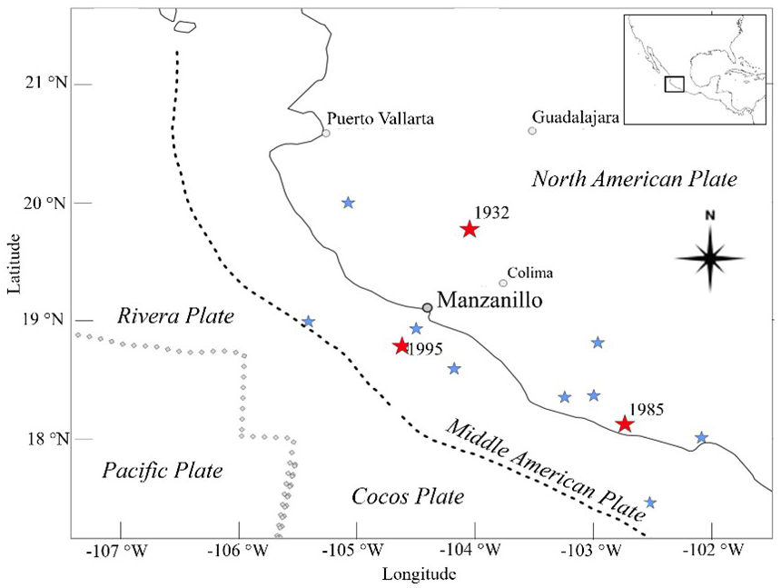
Figure 2Seismic environment of the study area. Red stars indicate earthquakes M≥8.0; blue stars indicate earthquakes .
The urban area of Manzanillo and its commercial port are connected to the rest of Mexico via the Colima–Manzanillo, Manzanillo–Puerto Vallarta and Cuyutlán–Manzanillo highways. Part of the embankment on one of these main avenues was selected for the analyses performed in this research. The Boulevard Miguel de la Madrid runs parallel to Miramar Beach, which is on Santiago Bay, northwest of the city of Manzanillo (Fig. 3). This beach has attractive natural characteristics, perfect for practicing sun and beach recreation activities (Cervantes et al., 2015); the road has become a waterfront promenade, with several restaurants and access points to the beach along the road. This road also connects the communities of El Naranjo, in the west, and Colinas de Santiago, in the east. It is also an important public transport route, serving tourists and the labour force going to and from the restaurants, hotels and recreation facilities. Further west is Playa de Oro International Airport. This road is therefore a vital part of the infrastructure of the city, facilitating many socioeconomic activities.

The data on the topography and topology of the section of embankment analysed here were obtained in fieldwork carried out in 2021. A total of 24 topographic profiles along a 2 km long section were surveyed (Fig. 4). The surveying equipment (eSurvey E300 PRO + P8II GNSS; global navigation satellite system) was positioned at a control point to later link the collected data with the official datum. With a centimetre precision, post-processing of the data gave the coordinates of a geodesic point which served as a reference to carry out the topographic survey. Based on the geometric characteristics of these cross-sections and their relative importance, the cross-section shown in Fig. 5 was selected for the sequential earthquake–tsunami analysis. The soil-embankment system was modelled using a three-dimensional approach where the 20 m segment of the coastal profile selected was considered uniform. This was the section considered to have the most critical condition of the road due to the height and the slope of the embankment.
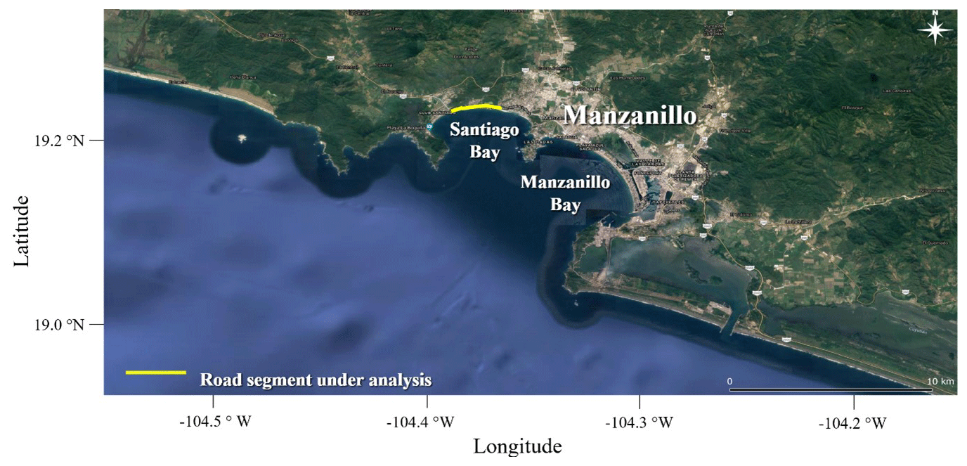
Figure 4Location of the road embankment analysed (© Google Earth).
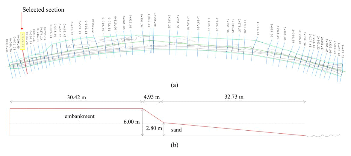
Figure 5(a) Cross-sections taken along the road and (b) the cross-section used in the analysis.
3.1 Seismic and geotechnical characterization of the study area
Manzanillo is in the northern part of the Sierra Madre del Sur mountain range. Geological studies by Tonatiuh Dominguez et al. (2017) state that granite intrusions, extrusive igneous outcrops and limestone deposits are found in the region. Deposits of clay and organic materials are also found in the two saltwater lagoons nearby. Sand deposits are found along the coast, and alluvial deposits are found around the igneous deposits (Fig. 6). Based on geophysical explorations at points S1 to S5 (Fig. 6), Tonatiuh Dominguez et al. (2017) show an in situ characterization of some dynamic properties, such as shear wave velocities and the shear wave velocities obtained from exploration at site 4, which is considered representative of characterizing sites with soil type B, where the section of the road embankment studied is located.
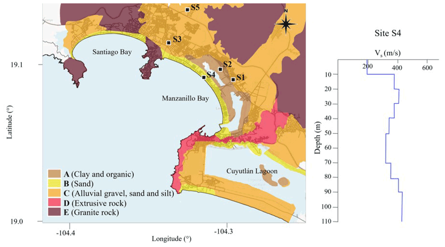
Figure 6Survey sites S1–S5. Geotechnical characterization of Manzanillo and Santiago bays obtained from Tonatiuh Dominguez et al. (2017) and shear wave velocity at site S4.
Manzanillo is located in the subduction zone between the Rivera and Cocos tectonic plates with the North American Plate. The rate of displacement at the contact surfaces is about 50 to 70 mm yr−1 (DeMets and Wilson, 1997), so the probability of severe earthquakes is high. Furthermore, in subduction zones, there is a high likelihood of tsunami occurrence, given the vertical displacement generated on the seabed, which can be several metres, extending over tens of thousands of square kilometres. Over time, numerous serious earthquakes have been recorded in this area, causing high-intensity ground movements, both in the continental region and along the coastline, as well as tsunami damage on the coast. According to historical records, at specific sites in this area the wave heights associated with tsunamis have reached 10 m. Tsunamigenic events occurring in this region are of Mw>8 magnitudes, among which are the 1787, 1932, 1985 and 1995 earthquakes in the study area.
3.2 Tsunamigenic seismic scenario
The seismic features were characterized using records from the seismic station MZ01 (Fig. 7) located on sandy deposits. It is the only station in free-field conditions in Manzanillo that was operating during the 1995 event (Mw=8.0). Table 1 summarizes the characteristics of the event. Figure 7 shows the location of station MZ01 and the epicentre of the 1995 event. Figures 8 and 9 show the acceleration time histories and their corresponding response spectra for each parameter measured at station MZ01.
Table 1Characteristics of the 1995 Manzanillo earthquake and the MZ01 station record.
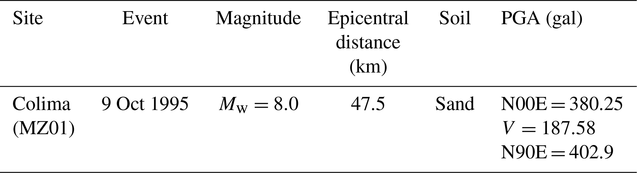
PGA: peak ground acceleration.
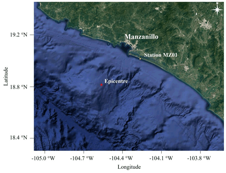
Figure 7Location of the seismic station MZ01 and the epicentre of the 1995 Manzanillo earthquake (Mw=8) event (© Google Earth).
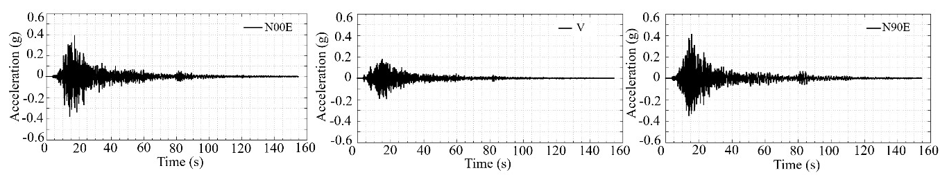
Figure 8Acceleration time histories at station MZ01 during the 1995 Manzanillo earthquake (Mw=8.0).
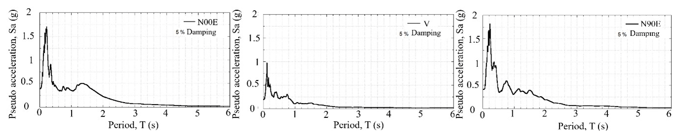
Figure 9Response spectra from the time histories recorded at station MZ01 during the 1995 Manzanillo earthquake (Mw=8.0).
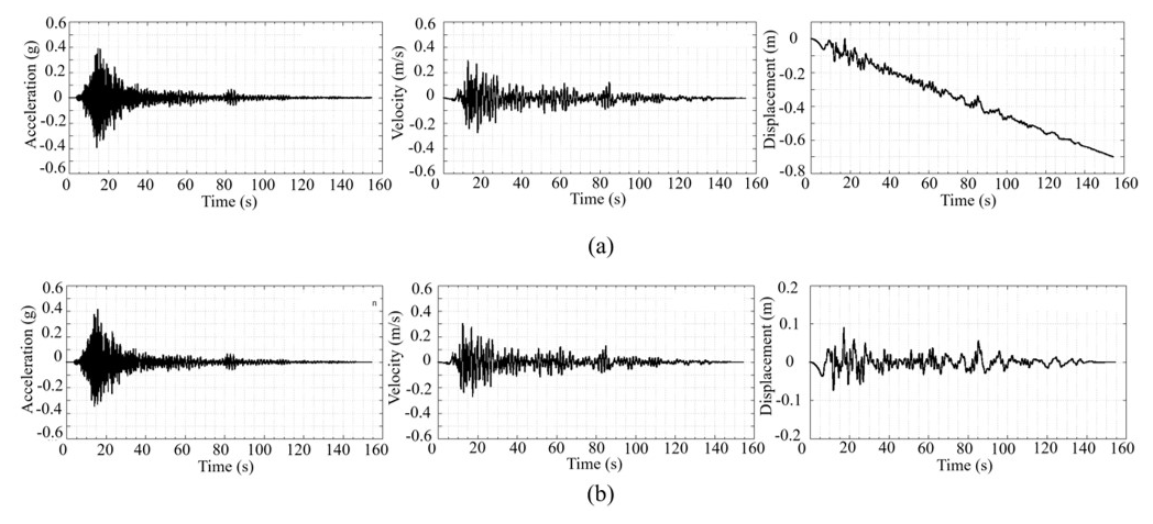
Figure 10Acceleration, velocity and displacement time histories (a) without baseline correction and (b) with baseline correction.
To perform the analysis, the record of the N90E component showing the larger accelerations and pseudo accelerations was selected. The acceleration time history was baseline-corrected to avoid residual velocities or displacements at the end of the movement, which could be confused with permanent displacements. Figure 10a and b show the acceleration, velocity and displacement histories before and after correction, respectively.
To simulate wave propagation during the earthquake, the selected acceleration history (N90E) was deconvolved using the soil profile of site S4 (Fig. 6), with the code SHAKE (Schnabel, 1972), which determines the vertical propagation of shear waves in a horizontally stratified semi-infinite soil deposit. Subsequently, the deconvolved earthquake was propagated again upward to verify that the propagation of the deconvolved and the recorded history are consistent. Figure 11 presents the comparison between the recorded and calculated response spectrum.
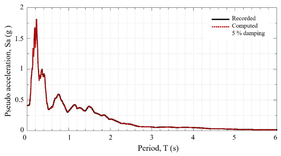
Figure 11Comparison between the recorded and calculated spectrum after the propagation of the deconvolved earthquake.
3.3 Step 1: seismic response
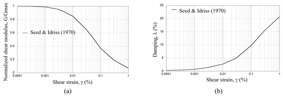
To simulate seismic wave propagation, during the earthquake, a site response analysis was performed using the N90E acceleration history. The record was deconvolved and propagated through the soil profile of the S4 site, performing a one-dimensional deterministic analysis. In this way, a first approximation of the expected dynamic amplification in the soil deposit was obtained, which is useful prior to the non-linear analysis in the time domain. This analysis also allows for the maximum dynamic shear stresses in the soil to be obtained, which are used to estimate the liquefaction potential in the simplified methods. Since dynamic laboratory tests were not performed on samples obtained near the study area, it was considered appropriate to assume the damping curves and shear stiffness modulus ratio presented by Seed and Idriss (1970) for sands (Fig. 12).
The stress history was determined and transformed into an equivalent number of cycles of uniform shear stress. In this way, the intensity and duration of ground motions are considered, as well as the variations in shear stress with depth. For practical purposes, the equivalent number of cycles of shear stress τav can be estimated as 65 % of the maximum stress τmax (Seed and Idriss, 1970) (Fig. 13).
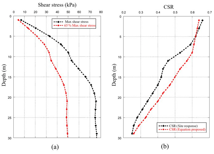
Figure 13(a) Maximum shear stress profile for the study site and (b) cyclic stress ratio profile, using the equation proposed by Seed and Idriss (1970) and the site response analysis.
The number of equivalent stress cycles Neq depends on the magnitude and duration of the earthquake. Seed et al. (1975) applied a weighting procedure to establish a uniform number of cycles of shear stress Neq (with an amplitude of 65 % of the maximum cyclic shear stress τcyc=0.65τmax) that would produce an equivalent pore pressure, where the number of cycles of uniform shear stress increases with increasing magnitude of the earthquake. For the case study, an earthquake magnitude Mw=8.0 corresponds to an equivalent number of cycles of uniform shear stress equal to 21 (Fig. 14).
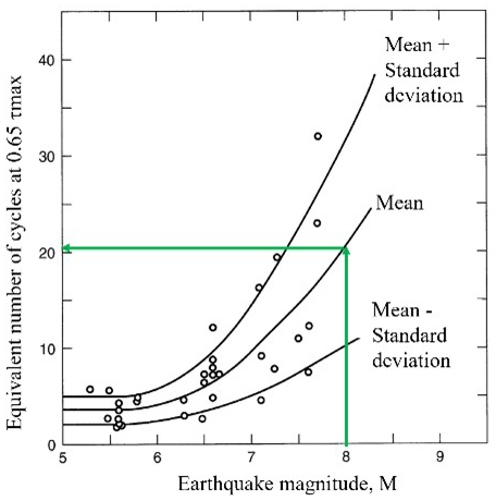
Figure 14Equivalent number of uniform cyclic loading Neq for different seismic magnitudes (Martin et al., 1975).
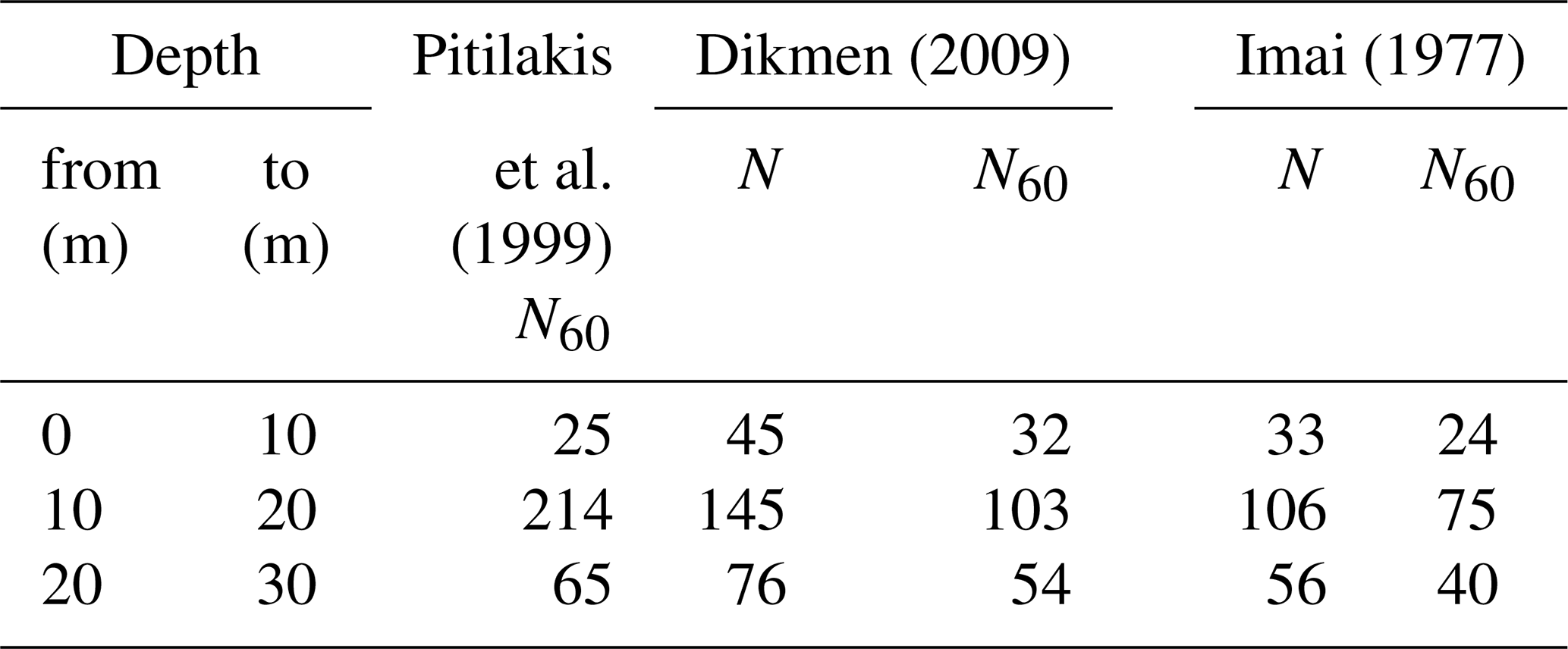
The liquefaction potential of the soil was evaluated using the cyclic stress criterion (Kramer, 1996; Seed and Idriss, 1970). One of the most common methods to evaluate liquefaction resistance is based on standard penetration tests (SPTs). This criterion uses the cyclic resistance ratio (CRR) from blow counts from the SPT, corrected to 60 % of the energy N60. Thus, according to the shear wave velocity profile of the study site, N60 was estimated using the expressions and parameters shown in Tables 2 and 3, obtaining N60=27, for the first 10 m of depth.
Table 2Correlations to estimate shear wave velocity.
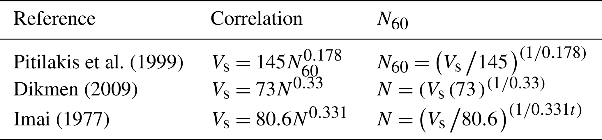
N: SPT blow counts, N60: blow counts 60 % energy corrected.
The safety factor against liquefaction for the embankment SFl was calculated based on the critical strength ratio (CSR), which was derived from the site response analysis (Table 4). A correction factor for the magnitude of the earthquake was applied. The CRR was obtained using the Robertson and Wride (1998) approximation, and the magnitude correction factor (MSF), proposed by Andrus and Stokoe (1999), was considered through the following equations:
The preliminary result shows that in the first 10 m of the profile there is the potential for soil liquefaction (Tables 5 and 6).
Table 4Safety factor against liquefaction.
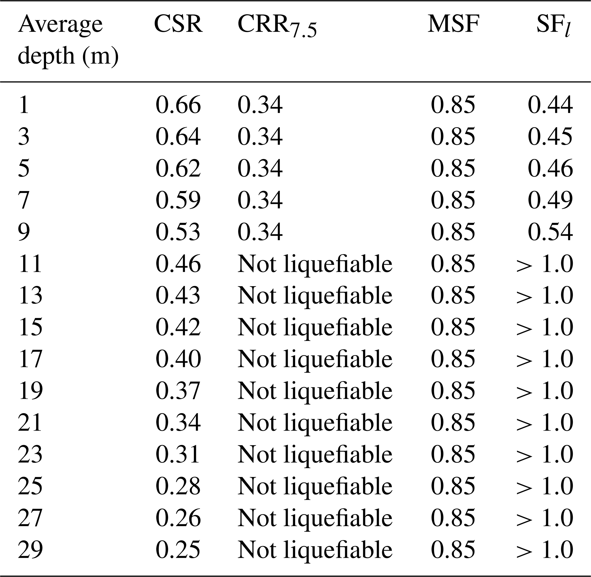
CSR: critical strength ratio, CRR7.5: cyclic resistance ratio, MSF: magnitude correction factor, SFl: safety factor against liquefaction.
The seismic response of the embankment was evaluated using a three-dimensional finite-difference simulation. This was carried out using the Finn et al. (1977) constitutive model for liquefiable soils, available in the software programme FLAC3D (Fast Lagrangian Analysis of Continua in 3 Dimensions) for the site response analyses of the slope and to account for soil non-linearities and loss of strength associated with pore pressure generation during cyclic loading (Fig. 15). For monotonic loading, an elastoplastic Mohr–Coulomb failure criterion was used that enables horizontal and vertical accelerations, displacements, shear forces, and pore pressure to be obtained. The model was composed of 13 632 elements and 16 083 nodes. The dimension of the element was selected based on the geometry and thicknesses of the soil layers. However, numerical distortion of the propagating wave can occur in a dynamic analysis as a result of the modelling conditions (Itasca Consulting Group, 2009). To represent wave transmission accurately, Kuhlemeyer and Lysmer (1973) suggest keeping the size of the spatial element Δl less than of the wavelength associated with the highest-frequency component of the input wave that contains significant energy fmax (i.e. ), where the shortest wavelength λ is obtained from . In the case study, the smallest average shear wave velocity Vs of the site corresponds to that of the first stiff soil layer (i.e. shear wave velocity is around 260 m s−1 in the first 10 m layer), while the highest excitation at which the energy is concentrated is about 1–5 Hz. Then, λ varies between 260 and 52 m approximately. The maximum spectral responses of the excitation occur even at higher frequencies (i.e. 0.5 and 10 Hz) as shown in Fig. 16. Hence, a Δl of 2 m was deemed appropriate. In previous research, using equivalent linear properties (Mayoral et al., 2015, 2016, 2017a, b), meshes with element sizes of 2 m showed good agreement between finite-difference models developed with FLAC3D and SHAKE.
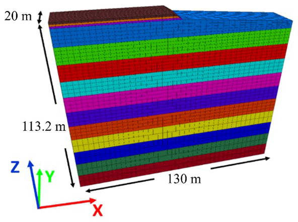
Figure 15Soil profile and road embankment in the three-dimensional finite-difference model. Each colour represents soil layers according to depths indicated in Table 5.

Table 5Soil characteristics.
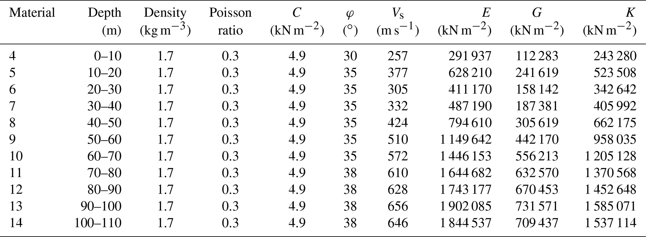
C: soil shear strength, ϕ: friction angle, Vs: shear wave velocity, E: Young's modulus, G: shear stiffness, K: constraint modulus.
Table 6Embankment characteristics.
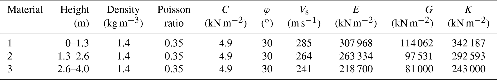
C: soil shear strength, ϕ: friction angle, Vs: shear wave velocity, E: Young's modulus, G: shear stiffness, K: constraint modulus.
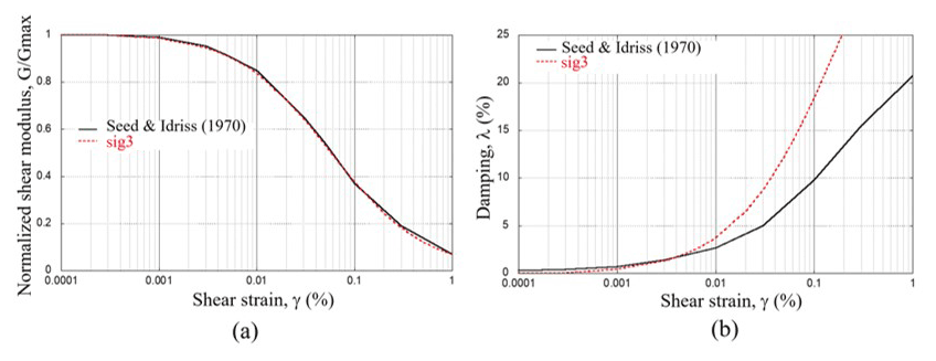
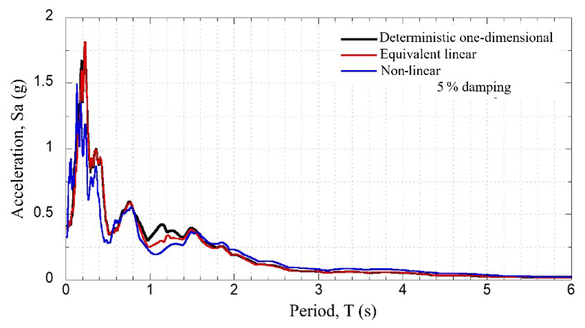
For calibration purposes, one-dimensional models were developed with the programme FLAC3D to solve the equation of motion in the time domain, considering both equivalent linear and non-linear properties, and the results were compared with those obtained in the frequency domain, with the programme SHAKE (Fig. 17). The sig3 model available in FLAC was used to approximately represent soil non-linearity. Thus, the sig3 hysteretic model was used to address the variation in the stiffness modulus and the damping ratio during the seismic event. This model considers an ideal soil, in which the stress depends only on the deformation and not on the number of cycle loads. With these assumptions an incremental constitutive relationship of the degradation curve can be described by , where τn is the normalized shear stress, γ is the shear strain and is the normalized secant modulus. The sig3 model is defined using the following expression:
where L is the logarithmic deformation, defined as L=log 10(γ), and the parameters a, b and x0, used by the sig3 model, were obtained through an iterative process, in which the modulus degradation curves were fitted with the model. The corresponding damping is given directly by the hysteresis loop during cyclic loading. For the case study, the parameters a, b and x0 take the values 1.014, −0.50 and −1.25, respectively. Figure 17 shows a comparison between the curves used in the deterministic unidimensional model (Seed and Idriss, 1970) and those obtained with the sig3 model. Figure 18 shows a comparison between the response spectra calculated on the surface with the deterministic one-dimensional model, the equivalent linear FLAC3D and the non-linear FLAC3D. Good agreement between the results was observed.
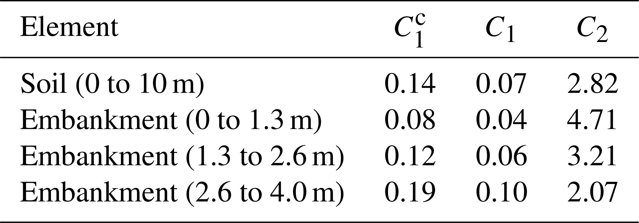
For the three-dimensional model, the Finn–Byrne model was used to evaluate the liquefaction potential. This model is defined as
where Δεvd is the decrease in volume per half cycle of deformation, γ is the shear strain, and C1 and C2 are constants that can be calculated as
These parameters, presented in Table 7, were calculated using the average values of (N1)60, for the first 10 m of soil and the embankment.
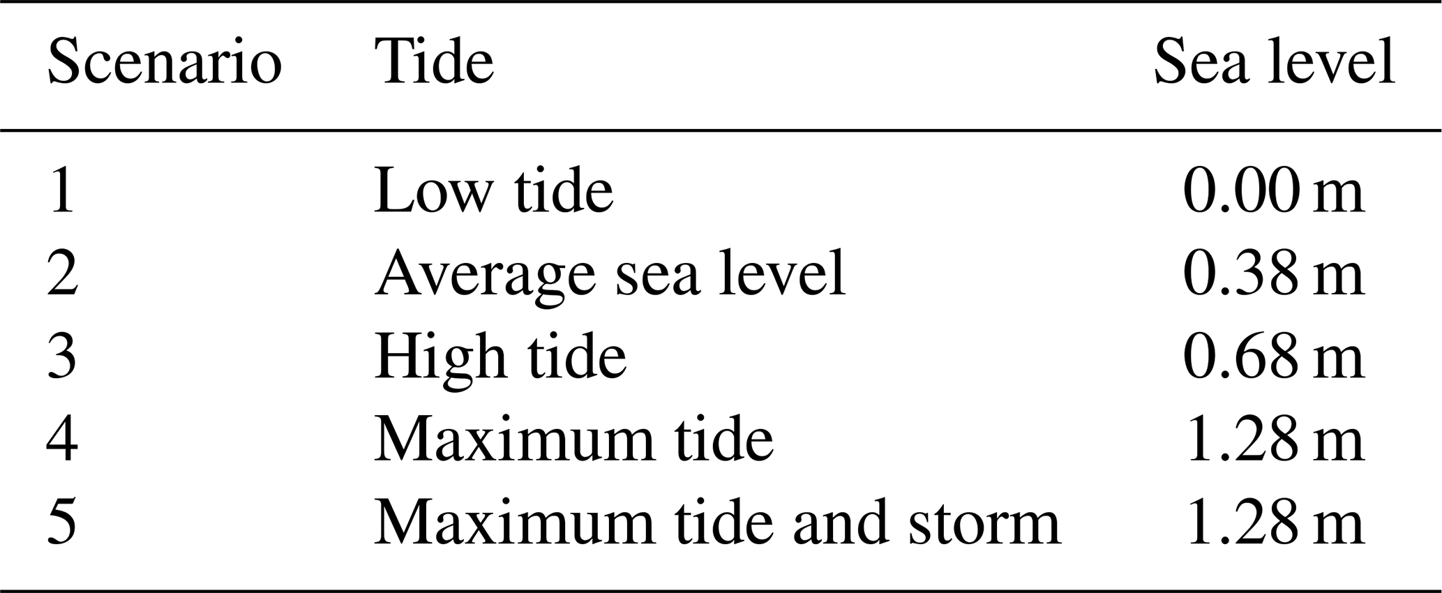
Five scenarios were considered to assess the seismic performance of the road embankment, considering the variations in sea level registered in the study area, as well as the case of high tide, and soil saturation due to rain (Table 8 and Fig. 19).
Seven control points were established in the model to obtain the soil behaviour parameters. Control points were located along the fault surface, at the toe of the embankment, at the highest point of the embankment and within the soil deposit (Fig. 19). Using the concept of static safety factor SFs, prior the application of the seismic loading, the general stability of the embankment under static conditions was evaluated for each scenario. SFs was above 2 in all the scenarios considered. The static safety factor was computed based on the concept of the strength over demand concept.
Next, an analysis of the seismic response was performed applying the N90E acceleration history (Fig. 11). It was observed that the largest vertical displacement, =73 cm, was recorded in scenario 5, on the crest of the embankment. Figure 20 presents the results of vertical displacement for scenarios 4 and 5 at the end of the earthquake. Figure 21 gives the results of the horizontal displacement for the same cases. The largest horizontal displacement was observed in scenario 5, =51 cm. Important vertical displacements of the soil were observed, as well as a tendency of lateral displacement of the body of the slope, increasing with depth.
At the control points, Fig. 22 shows the pore pressure ratio ru obtained for each scenario. A rise in pore pressure was observed at points G and F, in all scenarios. However, with the increase in the sea level, the higher pore pressure ratio at point D, located at the toe of the slope, continues to increase in scenarios 3 and 4 and reaches values above 0.7 in scenario 5, where an additional increase in this ratio was observed at point E, located on the failure surface of the slope.
3.4 Step 2: simulation of tsunami and wave propagation
The tsunami simulation was carried out using the model implemented in the GeoClaw code (Berger et al., 2011), which is based on solving the non-linear shallow-water equations through the numerical method of finite volumes, using adaptive mesh refinement to model small-scale features of the bathymetry as well as structures and coastal elements on the scale of metres (LeVeque et al., 2011). The shallow-water equations are the standard model used for transoceanic tsunami propagation as well as for local inundation (e.g. Yeh et al., 1994; Titov and Synolakis, 1995, 1998). In one space dimension these are
where g is the gravitational constant, h(x,t) is the fluid depth and u(x,t) is the vertically averaged horizontal fluid velocity. The function B(x) is the bottom surface elevation relative to mean sea level. Where B<0, this corresponds to submarine bathymetry, and where B>0, it corresponds to topography. GeoClaw code implementation allows for the bathymetry and topography to be time-dependent by solving the two-dimensional shallow-water equations (LeVeque et al., 2011):
where and are the depth-averaged velocities in the two horizontal directions and is the topography.
Table 9Fault characteristics of the 1995 Manzanillo earthquake.
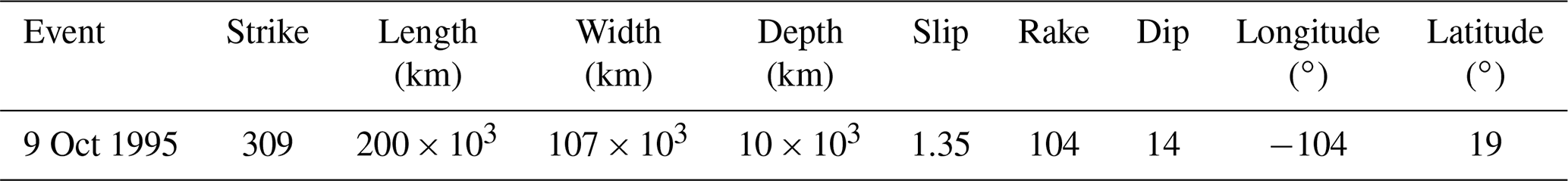
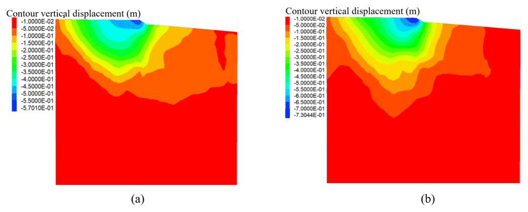
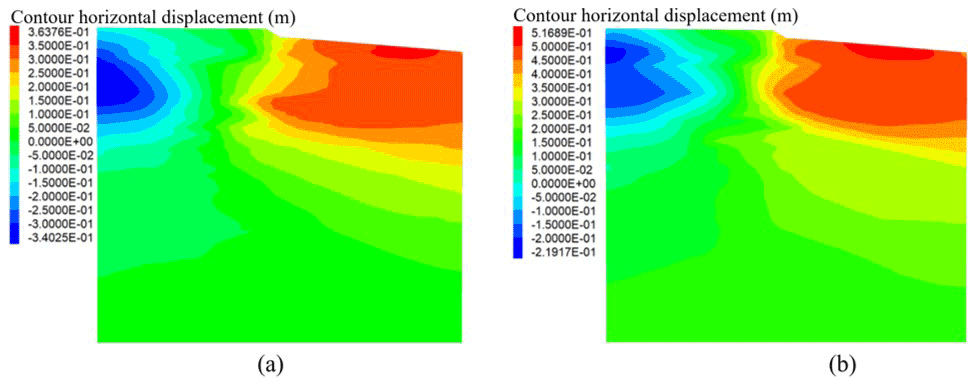
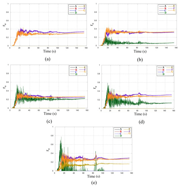
Figure 22Variations in pore pressure ratios in scenarios (a) 1, (b) 2, (c) 3, (d) 4 and (e) 5.
The bathymetric and topographic information used was obtained from the GEBCO (General Bathymetric Chart of the Oceans) database, with a resolution of 15 arcsec. A mesh of 129 600 cells was used, applying three levels for mesh refinement, with the finest grids used near the embankment segment, where the grid resolution was 210 m. Considering the characteristics of the fault mechanism of the 1995 Manzanillo earthquake (Table 9), the Okada (1995) fault model was used to estimate the vertical displacement on the seabed caused by the seismic event.
Based on the calculated deformations and the characteristics of the earthquake, a tsunami wave propagation model was run for a simulation period of 1 h, beginning 15 min after the start of the earthquake. Figure 23 shows the simulation results for 1 min. A 1 h simulation period was found for the case study analysed according to records of the duration of the event regarding the wave arriving times (García et al., 1997; Borrero et al., 1997). However, for other cases, longer simulation times could be considered, such as those recommended by ASCE (Robertson, 2017). The authors acknowledge that the grid resolution of the propagation model is a possible research topic for the future. However, a higher resolution was not possible at the time the model was developed. The improvement in the grid spacing would help to reduce uncertainties in the expected flood elevations.
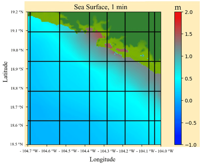
Figure 23Sea surface elevation obtained after a simulation time of 1 min.
Wave speeds and elevations were obtained at five virtual gauges in Santiago Bay, near the road embankment studied. These are shown in Table 10 and Fig. 24. Figure 25 shows the change in bathymetry at the gauge locations and the free sea surface elevation, respectively. Figure 26 shows the free sea surface elevation, the wave velocity components u and v at the gauge nearest to the coast, and the wave speed s.
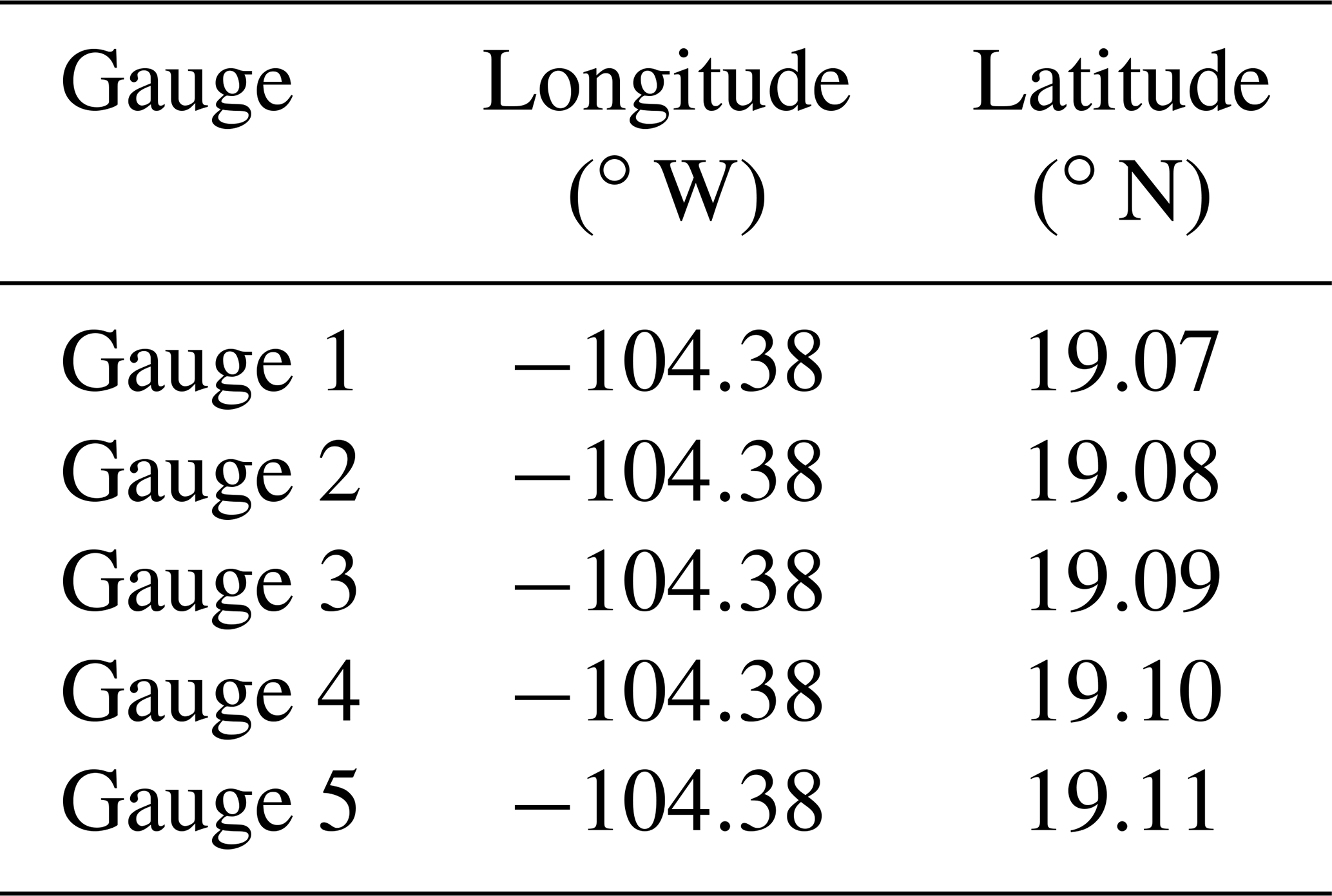
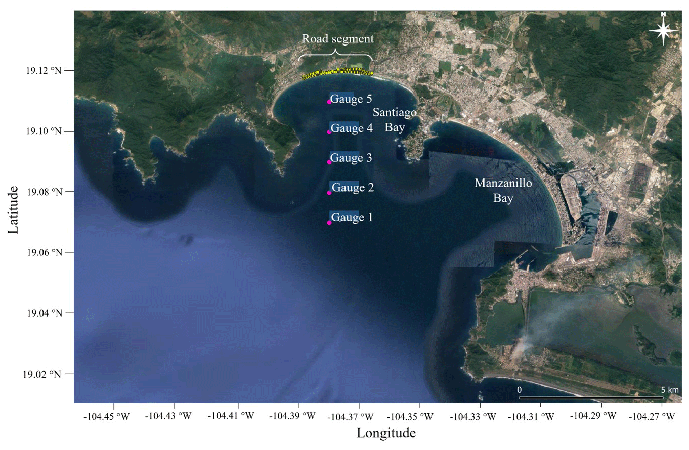
Figure 24Location of gauges used to obtain the free sea surface elevations and speeds in the simulation (© Google Earth).
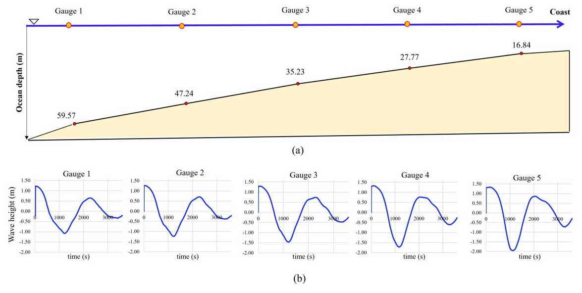
Figure 25(a) Ocean depths at the gauge locations (top) and (b) wave height distribution obtained during the simulation (bottom).
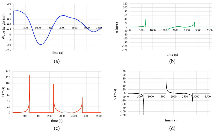
Figure 26For the gauge nearest to the coast (gauge 5): (a) free sea surface elevation, (b) horizontal velocity u, (c) wave speed s and (d) vertical velocity v.
It is worth mentioning that the maximum flood levels obtained coincide with the visual data reported by Avila-Armella et al. (2005).
3.5 Step 3: earthquake–tsunami response
Applying a smooth particle hydrodynamics approach, wave-induced hydrodynamic pressures associated with tsunami inundation at the study site were determined over the cross-section of Fig. 5. The hydrodynamic conditions of the simulation reproduce the flow velocities and elevation of the free sea surface of indicator 5, the closest to the coast (Fig. 26). The smooth particle hydrodynamics (SPH) model used is DualSPHysics, which has been widely used for hydrodynamic forces and to model complex fluid flows (González-Cao et al., 2019; Ye et al., 2019).
3.5.1 Validation
To validate the numerical approach, the experimental and numerical model of St-Germain et al. (2012) was reproduced, comparing water elevations of the incident wave in two control gauges. A tank 13.17 m long, 2.7 m wide, divided into two sections, and 1.4 m in height (Fig. 27) was considered. The model is made up of a dam break, consisting of a block of water of 0.85 m height that is released at time 0 through a swinging gate to travel towards the outflow.
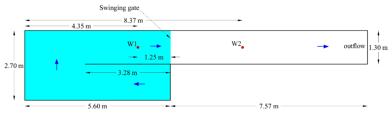
Figure 27Experimental model of St-Germain et al. (2012).

Figure 28Water heights at points W1 and W2 (St-Germain et al., 2012).
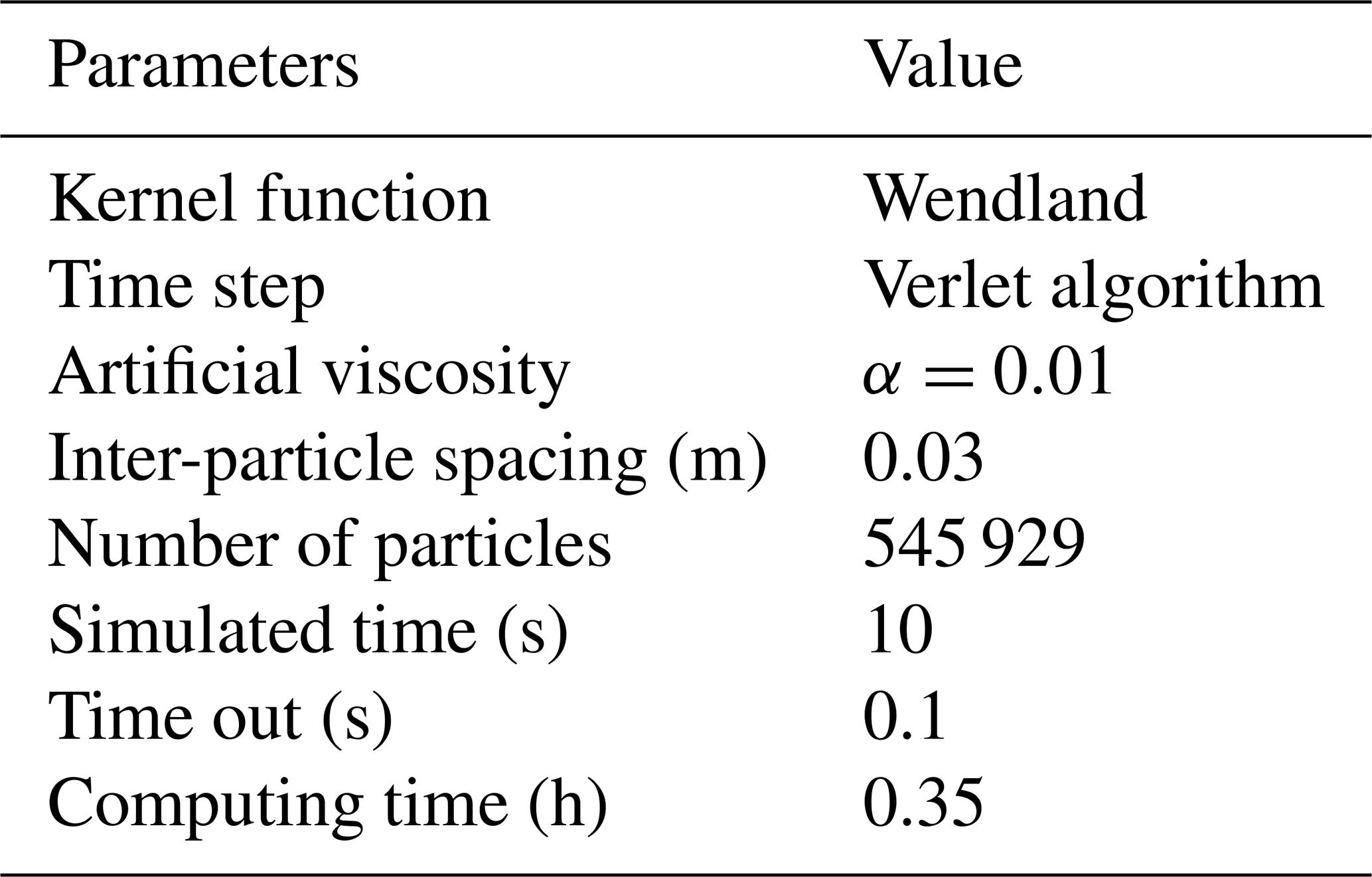
The validation SPH simulation parameters are shown in Table 11.
Table 11Parameters and main characteristics of the SPH simulation.
The simulation results are water heights at points W1 and W2 (Fig. 28). The standard deviation of the DualSPHysics model with respect to the experimental model is 5.4 cm for W1 and 5.2 cm for W2, which are 6.38 % and 6.16 % with reference to the initial height of the water. The standard deviation of DualSPHysics with respect to the numerical model of St-Germain et al. (2012) is 2.9 cm for W1 and 3.5 cm for W2, 3.4 % and 4.1 % concerning the initial height of the water.
3.5.2 Analysis of inter-particle spacing sensitivity
A simulation resolution analysis was performed for the SPH model. The resolution used was the initial size of the lattice nodes of the fluid particles and the fixed particles, defined as inter-particle spacing (dp). The simulation was made through tests with five different inter-particle spacings to obtain the resolution that allows for a convergence in the results with a lower computational cost (runtime).
The hydrodynamic pressures at the position x=10 m, z=2.1 m of the different resolutions (dp = 0.1, 0.2, 0.3, 0.4, 0.5, 0.6 and 0.7 m) were compared. The agreement of the results obtained with different resolutions is quantified by taking as reference the data series of the finest resolution of dp = 0.1 m, by means of the normalized standard deviation (σn), the centred root-mean-square deviation (RMSD) and the correlation (R), as shown in the Taylor diagram of Fig. 29 (as applied in González-Cao et al., 2019, and Klapp et al., 2020).

Figure 29Taylor diagram of hydrodynamic pressures at x=10 m and z=2.1 m, taking as reference the data series of the finest resolution of dp = 0.1 m.
Details of the resolution, runtime and number of simulated particles are shown in Fig. 30. The parameters and main characteristics of the simulations are shown in Table 12. The simulations were run on an Nvidia 1650 graphics processing unit (GPU).
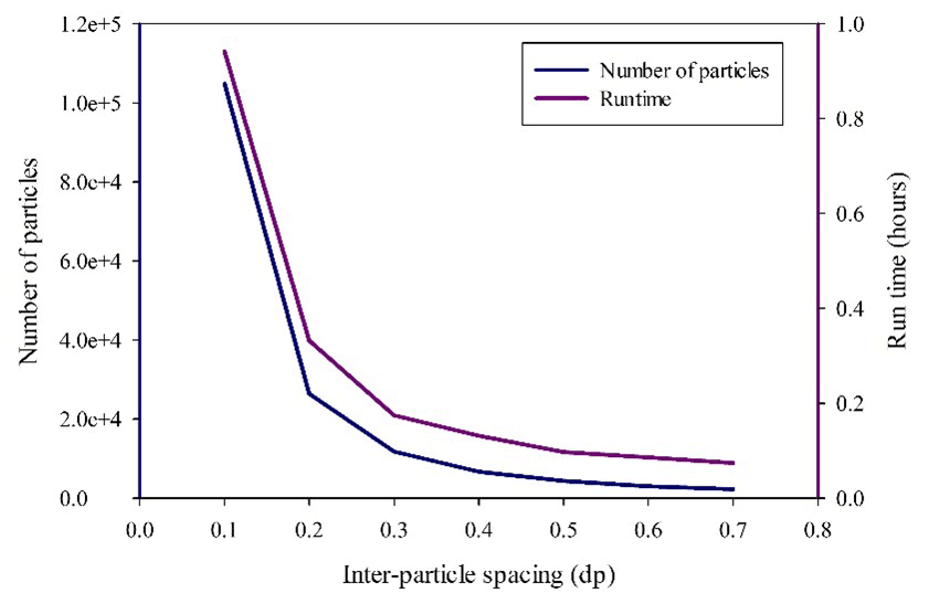
Table 12Parameters and main characteristics of the SPH simulation.
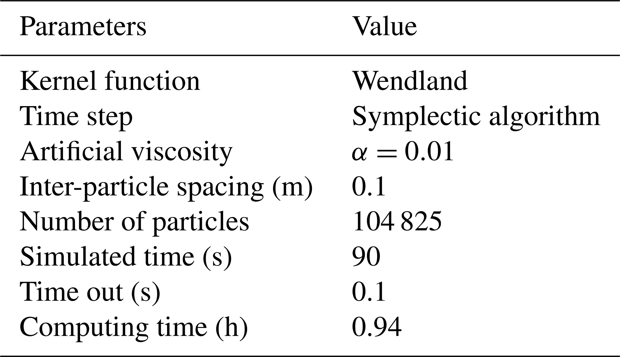
The results of the inter-particle spacing sensitivity analysis show that for all resolutions the correlation is greater than 95%, and that improves when the resolution is finer. However, a resolution greater than 0.1 m may not significantly improve the convergence of the results and may increase the computation time. Therefore, a resolution of 0.1 m with a particle number of 104 825 and a computation time of 0.94 h was selected.
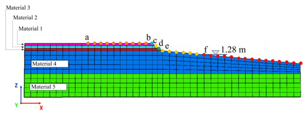
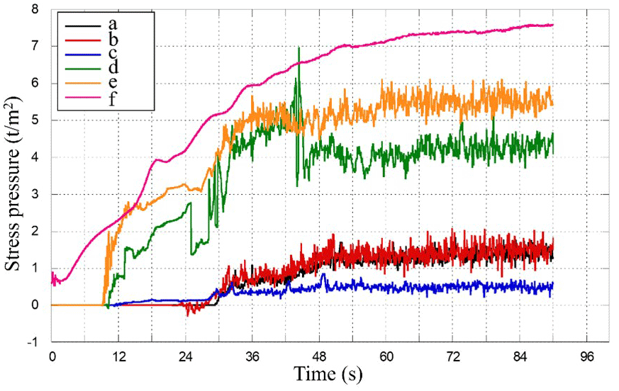
Figure 31 shows the pressures acting on the road embankment, and Fig. 32 shows the pressure evolution at points a–f, obtained in the first 90 s of loading, corresponding to the wave colliding with the slope of the embankment.
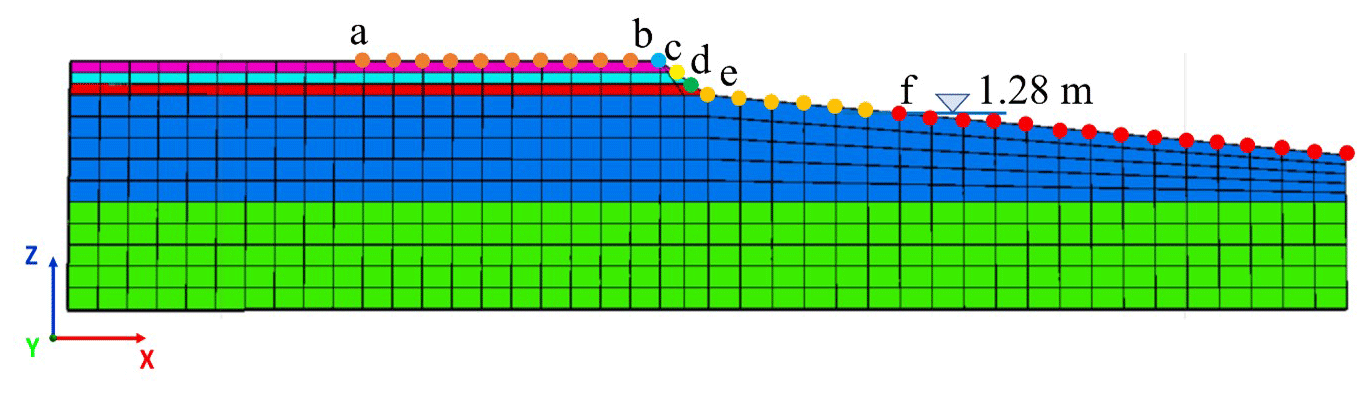
Figure 31Initial sea level and control points considered for the earthquake–tsunami loading analysis.
The wave-induced behaviour at the embankment was analysed, applying the same time step numerical approach of step 1 and the conditions of scenario 5, with an initial maximum tide of 1.28 m and saturated soil. From the results obtained in steps 1 and 2, the corresponding wave elevation of 1.5 m was modelled. In the model, the hydrodynamic pressures, pore pressures and incremental hydrostatic vertical loading were applied until the steady state in each of the loading points was reached.
Figure 33 shows the hydrostatic and hydrodynamic loading conditions applied at 50 s. The resulting vertical and horizontal displacements and the safety factor (i.e. capacity over demand) obtained from steady-state loading conditions are shown in Figs. 34 to 36.
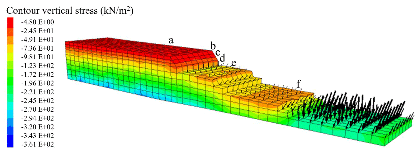
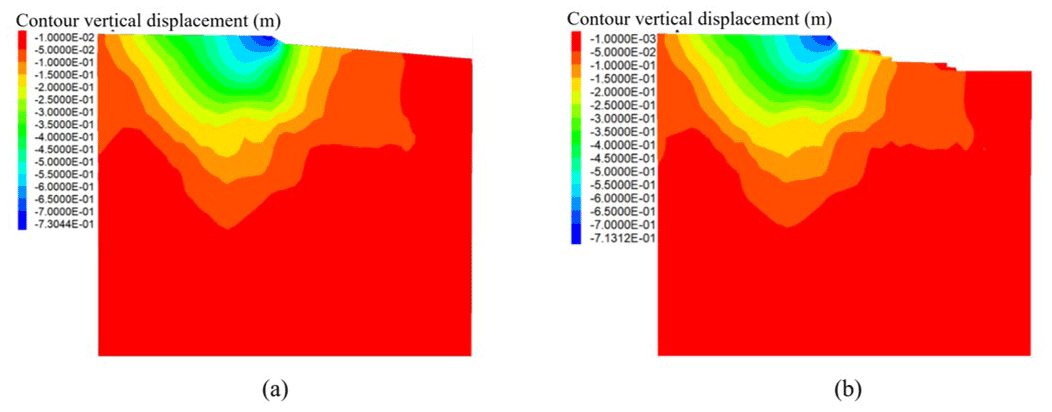
Figure 34Vertical displacements contours in metres (a) after seismic loading and (b) after tsunami loading.
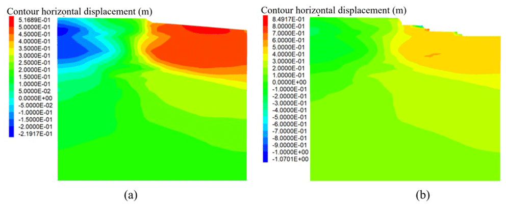
Figure 35Horizontal displacement contours in metres (a) after seismic loading and (b) after tsunami loading.
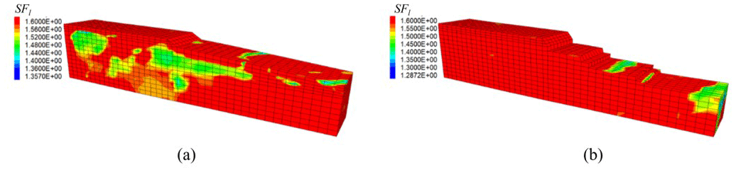
Figure 36Safety factor versus liquefaction (a) after seismic loading and (b) after tsunami loading.
The analysis shows that the main effects induced by wave loading are the horizontal displacement of the beach slope, reaching 0.8 m near point f. No major impacts were seen in the road embankment, where both vertical and horizontal displacements and the liquefaction safety factor show minor variations. However, there was a loss of granular material due to excessive ground deformation in the beach area. This effect was simulated following a time step approach, where zones of the mesh that reach a deformation of 2 m were removed from the model. The hydrodynamic loads were applied to the remaining mesh, which allowed the incremental unloading of the unstable areas in the sand found on the beach slope. The coupled effect of liquefaction and a tsunami could potentially lead to a loss of functionality of the road associated with an approximate 0.7 m displacement of the slope.
A sequential methodology was implemented to analyse the response of transportation infrastructure in an earthquake–tsunami. The methodology was applied for Manzanillo, Mexico, where the behaviour of a section of a road embankment was analysed, considering the accumulated effects of the earthquake in terms of horizontal and vertical displacements and those induced by an increase in sea level after the earthquake. In the case study, different scenarios were analysed depending on the initial elevation of the sea. The seismic response of the embankment showed that the most critical condition occurred in the scenarios of maximum high tide and maximum high tide with saturated soil. In these scenarios the vertical displacements were 0.57 and 0.73 m, respectively, both of which occurred at the embankment crest. The vertical and horizontal displacements can be interpreted as a failure of the embankment, in the sense that they may imply loss of functionality, since these give a 20 % reduction in the height of the structure.
The simulation of wave propagation of a tsunami showed that the level of the free sea surface could increase 1.5 m in the Manzanillo Bay area (Avila-Armella et al., 2005). Further analysis of the earthquake–tsunami behaviour showed that for the scenario of maximum high tide and saturated soil, the highest variation in the horizontal displacements in the ground between the stage at the end of the earthquake and the stage at the end of tsunami-induced flooding is seen on the beach slope. In the case study, the sequential model shows that seismic loading causes the greatest effects in pore pressure increase and in ground failure due to vertical and horizontal displacements in the embankment.
The sequential approach presented allows for soil displacements and strength to be accurately quantified, as well as pore pressure increase derived from an earthquake. The effects also couple with the tsunami arrival, which is not captured in decoupled models. The evaluation of these potential cumulative impacts provides additional information for the design and planning of more sustainable and resilient transportation infrastructure. The method presented is applicable to any coast, as long as there is sufficient information to characterize the site and structures, such as the seismic environment, geotechnics, bathymetry and structural systems. The degree of detail of the information required is of great importance to reduce uncertainty in the results.
From this study it is clear that, as in other parts of the world, the road network in Manzanillo has been built to improve communications but ignores many coastal processes, such as the potential presence of a tsunami. Moreover, this infrastructure was built on coastal dune ridges, inducing coastal squeeze, isolating ecosystems and increasing risk. The planning, design and construction of infrastructure in coastal areas susceptible to earthquakes and tsunamis should be rethought in order to make it compatible with natural processes and thus truly contribute to a better quality of life (Chávez et al., 2021; Silva et al., 2021). In the case of Manzanillo, a pile-driven road is probably a better option.
All data used to develop the numerical models presented are included in the paper. The authors are available for any specific requirement.
ARdlS and RS conceptualized the project and methodology. ARdlS, NPLA and AO acquired resources. MGVZ performed the measurements. ARdlS and OSAR analysed the data. ARdlS, OSAR and MGVZ wrote the draft. RS, EM, NPLLA and AO reviewed and edited the paper. SG reviewed and edited the paper.
The contact author has declared that none of the authors has any competing interests.
Publisher's note: Copernicus Publications remains neutral with regard to jurisdictional claims in published maps and institutional affiliations.
This paper was edited by Maria Ana Baptista and reviewed by three anonymous referees.
Akiyama, M., Frangopol, D. M., and Ishibashi, H.: Toward life-cycle reliability-, risk- and resilience-based design and assessment of bridges and bridge networks under independent and interacting hazards: emphasis on earthquake, tsunami and corrosion, Struct. Infrastruct. Eng., 16, 26–50, https://doi.org/10.1080/15732479.2019.1604770, 2020.
Altomare, C., Crespo, A. J. C., Domínguez, J. M., Gómez-Gesteira, M., Suzuki, T., and Verwaest, T.: Applicability of Smoothed Particle Hydrodynamics for estimation of sea wave impact on coastal structures, Coast. Eng., 96, 1–12, https://doi.org/10.1016/j.coastaleng.2014.11.001, 2015.
Andrus, R. D. and Stokoe, K. H.: Liquefaction resistance based on shear wave velocity, in: Technical Report NCEER-97-0022, NCEER Workshop on Evaluation of Liquefaction Resistance of Soils, Salt Lake City, UT, edited by: Youd, T. L. and Idriss, I. M., National Center for Earthquake Engineering Research, Buffalo, NY, 89–128, https://trid.trb.org/view/542968 (last access: 6 August 2022), 1999.
Argyroudis, S. and Kaynia, A. M.: Analytical seismic fragility functions for highway and railway embankments and cuts, Earthq. Eng. Struct. Dynam., 44, 1863–1879, https://doi.org/10.1002/eqe.2563, 2015.
Argyroudis, S. A. and Mitoulis, S. A.: Vulnerability of bridges to individual and multiple hazards- floods and earthquakes, Reliabil. Eng. Syst. Safe., 210, 107564, https://doi.org/10.1016/j.ress.2021.107564, 2021.
Attary, N., Van De Lindt, J. W., Barbosa, A. R., Cox, D. T., and Unnikrishnan, V. U.: Performance-Based Tsunami Engineering for Risk Assessment of Structures Subjected to Multi-Hazards: Tsunami following Earthquake, J. Earthq. Eng., 25, 2065–2084, https://doi.org/10.1080/13632469.2019.1616335, 2021.
Avila-Armella, A., Pedrozo-Acuna, A., Silva-Casarin, R., and Simmonds, D.: Prediction of tsunami-induced flood on the Mexican Pacific coast, Ingenieria Hidraulica en Mexico, 20, 5–18, 2005.
Berger, M. J., George, D. L., LeVeque, R. J., and Mandli, K. T.: The GeoClaw software for depth-averaged flows with adaptive refinement, Adv. Water Resour., 34, 1195–1206, https://doi.org/10.1016/j.advwatres.2011.02.016, 2011.
Bhattacharya, S., Hyodo, M., Nikitas, G., Ismail, B., Suzuki, H., Lombardi, D., Egami, S., Watanabe, G., and Goda, K.: Geotechnical and infrastructural damage due to the 2016 Kumamoto earthquake sequence, Soil Dynam. Earthq. Eng., 104, 390–394, https://doi.org/10.1016/j.soildyn.2017.11.009, 2017.
Borerro, J., Ortiz, M., Titov, V., and Synolakis, C.: Field survey of Mexican tsunami produces new data, unusual photos, EOS Trans. Am. Geophys. Union, 78, 85–88, 1997.
Briaud, J.-L. and Maddah, L.: Minimizing roadway embankment damage from flooding, Project 20-05 (Topic 46-16), Transportation Research Board, Washington, DC, https://doi.org/10.17226/23604, 2016.
Burns Patrick, O., Barbosa Andre, R., Olsen Michael, J., and Wang, H.: Multihazard Damage and Loss Assessment of Bridges in a Highway Network Subjected to Earthquake and Tsunami Hazards, Nat. Hazards Rev., 22, 05021002, https://doi.org/10.1061/(ASCE)NH.1527-6996.0000429, 2021.
Cervantes, O., Verduzco-Zapata, G., Botero, C., Olivos-Ortiz, A., Chávez-Comparan, J. C., and Galicia-Pérez, M.: Determination of risk to users by the spatial and temporal variation of rip currents on the beach of Santiago Bay, Manzanillo, Mexico: Beach hazards and safety strategy as tool for coastal zone management, Ocean Coast. Manage., 118, 205–214, https://doi.org/10.1016/j.ocecoaman.2015.07.009, 2015.
Chávez, V., Lithgow, D., Losada, M., and Silva-Casarin, R.: Coastal green infrastructure to mitigate coastal squeeze, J. Infrastruct. Preserv. Resil., 2, 7, https://doi.org/10.1186/s43065-021-00026-1, 2021.
Chinnarasri, C., Thanasisathit, N., Ruangrassamee, A., Weesakul, S., and Lukkunaprasit, P.: The impact of tsunami-induced bores on buildings, Proc. Inst. Civ. Eng.-Maritim. Eng., 166, 14–24, https://doi.org/10.1680/maen.2010.31, 2013.
Cubrinovski, M.: Liquefaction-Induced Damage in the 2010–2011 Christchurch (New Zealand) Earthquakes, in: International Conference on Case Histories in Geotechnical Engineering, 29 April–4 May 2013, Chicago, USA, 1–11, https://scholarsmine.mst.edu/icchge/7icchge/session12/1 (last access: 6 August 2022), 2013.
DeMets, C. and Wilson, D. S.: Relative motions of the Pacific, Rivera, North American, and Cocos plates since 0.78 Ma, J. Geophys. Res.-Solid, 102, 2789–2806, https://doi.org/10.1029/96JB03170, 1997.
Dikmen, Ü.: Statistical correlations of shear wave velocity and penetration resistance for soils, J. Geophys. Eng., 6, 61–72, https://doi.org/10.1088/1742-2132/6/1/007, 2009.
Dizhur, D., Giaretton, M., and Ingham, J. M.: Damage Observations Following the Mw 7.8 2016 Kaikoura Earthquake, in: International Conference on Earthquake Engineering and Structural Dynamics ICESD2017Reykjavík, 12–14 June 2017, Iceland, 249–261, https://icesd.hi.is/ (last access: 6 August 2025), 2019.
EQE International: The October 9, 1995 Manzanillo, Mexico earthquake: Summary of structural damage, A summary report, EQE International, 6–14, 1996.
Escudero Castillo, M., Mendoza Baldwin, E., Silva Casarin, R., Posada Vanegas, G., and Arganis Juaréz, M.: Characterization of Risks in Coastal Zones: A Review, CLEAN – Soil Air Water, 40, 894–905, https://doi.org/10.1002/clen.201100679, 2012.
Finn, W. L., Lee, K., and Martin, G.: An Effective Stress Model for Liquefaction, J. Geotech. Eng. Div.-ASCE, 103, 517–533, 1977.
García, H. J., Whitney, R. A., Guerrero, J. J., Gama, A., Vera, R., and Hurtado, F.: The October 9, 1995 Manzanillo, Mexico Earthquake, Seismol. Res. Lett., 68, 413–425, 1997.
Goda, K.: Multi-hazard parametric catastrophe bond trigger design for subduction earthquakes and tsunamis, Earthq. Spectra, 37, 1827–1848, 2021.
Goda, K., Petrone, C., De Risi, R., and Rossetto, T.: Stochastic coupled simulation of strong motion and tsunami for the 2011 Tohoku, Japan earthquake, Stoch. Environ. Res. Risk A., 31, 2337–2355, 2017.
Goda, K., De Risi, R., De Luca, F., Muhammad, A., Yasuda, T., and Mori, N.: Multi-hazard earthquake-tsunami loss estimation of Kuroshio Town, Kochi Prefecture, Japan considering the Nankai-Tonankai megathrust rupture scenarios, Int. J. Disast. Risk Reduct., 54, 102050, https://doi.org/10.1016/j.ijdrr.2021.102050, 2021.
González-Cao, J., Altomare, C., Crespo, A. J. C., Domínguez, J. M., Gómez-Gesteira, M., and Kisacik, D.: On the accuracy of DualSPHysics to assess violent collisions with coastal structures, Comput. Fluids, 179, 604–612, https://doi.org/10.1016/j.compfluid.2018.11.021, 2019.
Hasanpour, A., Denis, I., and Ian, B.: Coupled SPH–FEM Modeling of Tsunami-Borne Large Debris Flow and Impact on Coastal Structures, J. Mar. Sci. Eng., 9, 1068–1080, https://doi.org/10.3390/jmse9101068, 2021.
Iai, S.: Evaluation of performance of port structures during earthquakes, Soil Dynam. Earthq. Eng., 126, 105192, https://doi.org/10.1016/j.soildyn.2018.04.055, 2019.
Imai, T.: P and S wave velocities of the ground in Japan, in: Proc. 9th ICSMFE, Tokyo, 257–260, 2013.
Ishibashi, H., Akiyama, M., Frangopol, D. M., Koshimura, S., Kojima, T., and Nanami, K.: Framework for estimating the risk and resilience of road networks with bridges and embankments under both seismic and tsunami hazards, Struct. Infrastruct. Eng., 17, 494–514, https://doi.org/10.1080/15732479.2020.1843503, 2021.
Itasca Consulting Group: FLAC3D, Fast lagrangian analysis of continua in 3 dimensions, User's guide, Minneapolis, Minnesota, USA, 2009.
Jose, J., Choi, S.-J., Giljarhus, K. E. T., and Gudmestad, O. T.: A comparison of numerical simulations of breaking wave forces on a monopile structure using two different numerical models based on finite difference and finite volume methods, Ocean Eng., 137, 78–88, https://doi.org/10.1016/j.oceaneng.2017.03.045, 2017.
Kakderi, K. and Pitilakis, K.: Fragility Functions of Harbor Elements, in: SYNER-G: Typology Definition and Fragility Functions for Physical Elements at Seismic Risk: Buildings, Lifelines, Transportation Networks and Critical Facilities, edited by: Pitilakis, K., Crowley, H., and Kaynia, A. M., Springer Netherlands, Dordrecht, 327–356, https://doi.org/10.1007/978-94-007-7872-6_11, 2014.
Karafagka, S., Fotopoulou, S., and Pitilakis, K.: Analytical tsunami fragility curves for seaport RC buildings and steel light frame warehouses, Soil Dynam. Earthq. Eng., 112, 118–137, https://doi.org/10.1016/J.SOILDYN.2018.04.037, 2018.
Klapp, J., Areu-Rangel, O. S., Cruchaga, M., Aránguiz, R., Bonasia, R., Godoy, M. J., and Silva-Casarín, R.: Tsunami hydrodynamic force on a building using a SPH real-scale numerical simulation, Nat. Hazards, 100, 89–109, https://doi.org/10.1007/s11069-019-03800-3, 2020.
Koshimura, S., Hayashi, S., and Gokon, H.: The impact of the 2011 Tohoku earthquake tsunami disaster and implications to the reconstruction, Soils Foundat., 54, 560–572, https://doi.org/10.1016/j.sandf.2014.06.002, 2014.
Kramer, S. L.: Geotechnical earthquake engineering, Pearson Education India, 1996.
Kuhlemeyer, R. L. and Lysmer, J.: Finite element method accuracy for wave propagation problems, J. Soil Mech. Found. Div., 99, 421–427, 1973.
LeVeque, R. J., George, D. L., and Berger, M. J.: Tsunami modelling with adaptively refined finite volume methods, Acta Numerica, 20, 211–289, 2011.
Martin, G. R., Seed, H. B., and Finn, W. L.: Fundamentals of liquefaction under cyclic loading, J. Geotech. Eng. Div., 101, 423–438, 1975.
Maruyama, Y., Yamazaki, F., Mizuno, K., Tsuchiya, Y., and Yogai, H.: Fragility curves for expressway embankments based on damage datasets after recent earthquakes in Japan, Soil Dynam. Earthq. Eng., 30, 1158–1167, https://doi.org/10.1016/j.soildyn.2010.04.024, 2010.
Mayoral, J. M., Castañón, E., and Sarmiento, N.: Seismic response of high plasticity clays during extreme events, Soil Dynam. Earthq. Eng., 77, 203–207, 2015.
Mayoral, J. M., Argyroudis, S., and Castañon, E.: Vulnerability of floating tunnel shafts for increasing earthquake loading, Soil Dynam. Earthq. Eng., 80, 1–10, https://doi.org/10.1016/j.soildyn.2015.10.002, 2016.
Mayoral, J. M., Badillo, A., and Alcaraz, M.: Vulnerability and recovery time evaluation of an enhanced urban overpass foundation, Soil Dynam. Earthq. Eng., 100, 1–15, https://doi.org/10.1016/j.soildyn.2017.05.023, 2017a.
Mayoral, J. M., Castañón, E., and Albarrán, J.: Regional subsidence effects on seismic soil-structure interaction in soft clay, Soil Dynam. Earthq. Eng., 103, 123–240, https://doi.org/10.1016/j.soildyn.2017.09.014, 2017b.
McKenna, G., Argyroudis, S. A., Winter, M. G., and Mitoulis, S. A.: Multiple hazard fragility analysis for granular highway embankments: Moisture ingress and scour, Transport. Geotech., 26, 100431, https://doi.org/10.1016/j.trgeo.2020.100431, 2021.
NIBS: Users's manual and technical manuals, in: Report Prepared for the Federal Emergency Management Agency, National Institute of Building Sciences, Washington, DC, USA, https://www.fema.gov/sites/default/files/2020-09/fema_hazus_advanced-engineering-building-module_user-manual.pdf (last access: 7 August 2022), 2004.
Okada, M.: Tsunami observation by ocean bottom pressure gauge, in: Tsunami: progress in prediction, disaster prevention and warning, Springer, 287–303, https://doi.org/10.1007/978-94-015-8565-1_21, 1995.
Ovando-Shelley, E. and Romo, M.: Three Recent Damaging Earthquakes in Mexico, in: International Conference on Case Histories in Geotechnical Engineering, 13 April 2004, New York, https://scholarsmine.mst.edu/icchge/5icchge/ (last access: 7 August 2022), 2004.
Pitilakis, K., Raptakis, D., Lontzetidis, K., Tika-Vassilikou, T., and Jongmans, D.: Geotechnical and geophysical description of EURO-SEISTEST, using field, laboratory tests and moderate strong motion recordings, J. Earthq. Eng., 3, 381–409, 1999.
Robertson, C.: Overview and technical background to development of ASCE 7–16 Chapter 6, Tsunami Loads and Effects, in: 16th World Conference on Earthquake Engineering, 16WCEE, 9–13 January 2017, Santiago, Chile, https://www.wcee.nicee.org/wcee/article/16WCEE/WCEE2017-253.pdf (last access: 8 August 2022), 2017.
Robertson, P. K. and Wride, C.: Evaluating cyclic liquefaction potential using the cone penetration test, Can. Geotech. J., 35, 442–459, https://doi.org/10.1139/t98-017, 1998.
Rowell, M. and Goodchild, A.: Effect of Tsunami Damage on Passenger and Forestry Transportation in Pacific County, Washington, Transport. Res. Record, 2604, 88–94, https://doi.org/10.3141/2604-11, 2017.
Sarkis, A., Palermo, A., Kammouh, O., and Cimellaro, G.: Seismic resilience of road bridges: lessons learned from the 14 November 2016 Kaikōura Earthquake, in: Proceedings of the 9th International Conference on Bridge Maintenance, Safety, 9–13 July 2018, Melbourne, Australia, 9–13, 2018.
Schnabel, P. B.: SHAKE: A Computer Program for Earthquake Response Analysis of Horizontally Layered Sites, EERC Report 72-12, University of California, Berkeley, CA, USA, https://www.resolutionmineeis.us/documents/schnabel-lysmer-seed-1972 (last access: 8 August 2022), 1972.
Seed, H., Idriss, I., Makdisi, F., and Banerjee, N.: Representation of irregular stress time histories by equivalent uniform stress series in liquefaction analyses, EERC 75-29, Earthquake Engineering Research Center, University of California, Berkeley, https://pdfcoffee.com/eerc-75-29-pdf-free.html (last access: 7 August 2022), 1975.
Seed, H. B. and Idriss, I. M.: Analyses of ground motions at Union Bay, Seattle during earthquakes and distant nuclear blasts, Bull. Seismol. Soc. Am., 60, 125–136, https://doi.org/10.1785/BSSA0600010125, 1970.
Silva, R., Chávez, V., Bouma, T. J., van Tussenbroek, B. I., Arkema, K. K., Martínez, M. L., Oumeraci, H., Heymans, J. J., Osorio, A. F., Mendoza, E., Mancuso, M., Asmus, M., and Pereira, P.: The Incorporation of Biophysical and Social Components in Coastal Management, Estuar. Coasts, 42, 1695–1708, https://doi.org/10.1007/s12237-019-00559-5, 2019.
Silva, R., Martínez, M. L., van Tussenbroek, B. I., Guzmán-Rodríguez, L. O., Mendoza, E., and López-Portillo, J.: A Framework to Manage Coastal Squeeze, Sustainability, 12, 10610, https://doi.org/10.3390/su122410610, 2020.
Silva, R., Oumeraci, H., Martínez, M. L., Chávez, V., Lithgow, D., van Tussenbroek, B. I., van Rijswick, H. F. M. W., and Bouma, T. J.: Ten Commandments for Sustainable, Safe, and W/Healthy Sandy Coasts Facing Global Change, Front. Mar. Sci., 8, 616321, https://doi.org/10.3389/fmars.2021.616321, 2021.
St-Germain, P., Nistor, I., and Townsend, R.: Numericalmodeling of tsunami-induced hydrodynamic forces on onshore structures using SPH, in: Proc. 33rd Int. Conf. on Coastal Engineering, ASCE, Reston, VA, https://doi.org/10.9753/icce.v33.structures.81, 2012.
Titov, V. V. and Synolakis, C. E: Modeling of breaking and nonbreaking long-wave evolution and runup using VTCS-2, J. Waterway Port Coast. Ocean Eng., 121, 308–316, 1995.
Titov, V. V., and Synolakis, C. E.: Numerical modeling of tidal wave runup, J. Waterway Port Coast. Ocean Eng., 124, 157–171, 1998.
Tonatiuh Dominguez, R., Rodríguez-Lozoya, H. E., Sandoval, M. C., Sanchez, E. S., Meléndez, A. A., Rodríguez- Leyva, H. E., and Amelia Campos, R.: Site response in a representative region of Manzanillo, Colima, Mexico, and a comparison between spectra from real records and spectra from normative, Soil Dynam. Earthq. Eng., 93, 113–120, https://doi.org/10.1016/j.soildyn.2016.11.013, 2017.
Williams, J. H., Wilson, T. M., Horspool, N., Lane, E. M., Hughes, M. W., Davies, T., Le, L., and Scheele, F.: Tsunami impact assessment: development of vulnerability matrix for critical infrastructure and application to Christchurch, New Zealand, Nat. Hazards, 96, 1167–1211, https://doi.org/10.21203/rs.3.rs-1104603/v1, 2019.
Williams, J. H., Wilson, T. M., Horspool, N., Paulik, R., Wotherspoon, L., Lane, E. M., and Hughes, M. W.: Assessing transportation vulnerability to tsunamis: utilising post-event field data from the 2011 Tōhoku tsunami, Japan, and the 2015 Illapel tsunami, Chile, Nat. Hazards Earth Syst. Sci., 20, 451–470, https://doi.org/10.5194/nhess-20-451-2020, 2020.
Ye, T., Pan, D., Huang, C., and Liu, M.: Smoothed particle hydrodynamics (SPH) for complex fluid flows: Recent developments in methodology and applications, Phys. Fluids, 31, 011301, https://doi.org/10.1063/1.5068697, 2019.
Yeh, H., Liu, P., Briggs, M., and Synolakis, C.: Propagation and amplification of tsunamis at coastal boundaries, Nature, 372, 353–355, 1994.