the Creative Commons Attribution 4.0 License.
the Creative Commons Attribution 4.0 License.
 | 28 Jan 2022
Investigating the interaction of waves and river discharge during compound flooding at Breede Estuary, South Africa
Sunna Kupfer
Sara Santamaria-Aguilar
Lara van Niekerk
Melanie Lück-Vogel
Athanasios T. Vafeidis
Recent studies have drawn special attention to the significant dependencies between flood drivers and the occurrence of compound flood events in coastal areas. This study investigates compound flooding from tides, river discharge (Q), and specifically waves using a hydrodynamic model at the Breede Estuary, South Africa. We quantify vertical and horizontal differences in flood characteristics caused by driver interaction and assess the contribution of waves. Therefore, we compare flood characteristics resulting from compound flood scenarios to those in which single drivers are omitted. We find that flood characteristics are more sensitive to Q than to waves, particularly when the latter only coincides with high spring tides. When interacting with Q, however, the contribution of waves is high, causing 10 %–12 % larger flood extents and 45–85 cm higher water depths, as waves caused backwater effects and raised water levels inside the lower reaches of the estuary. With higher wave intensity, the first flooding began up to 12 h earlier. Our findings provide insights on compound flooding in terms of flood magnitude and timing at a South African estuary and demonstrate the need to account for the effects of compound events, including waves, in future flood impact assessments of open South African estuaries.
- Article
(10593 KB) - Full-text XML
- BibTeX
- EndNote


Floods, regardless of fluvial or oceanic origin, are among the world's most devastating coastal hazards, causing numerous deaths and large economic losses on an annual basis (Kirezci et al., 2020). Despite improved flood protection, forecasting, and warnings, flooding remains a growing threat due to the continued global coastal urbanization which results in rapid population growth, economic development, and land use change (Brown et al., 2018; Hallegatte et al., 2013; Hanson et al., 2011). Moreover, the accelerating rate of sea-level rise (SLR) may cause historically rare floods to become common by the end of the century (Vitousek et al., 2017). In coastal areas, the interactions of oceanographic, hydrological, and meteorological phenomena can lead to extensive flooding. Particularly in estuaries, such floods can result from combined spring tides and extreme wave or storm surge conditions occurring simultaneously with high river discharge (Kumbier et al., 2018; Olbert et al., 2017; Ward et al., 2018). These events are commonly referred to as compound flood events. Definitions of compound events have evolved in recent years (Leonard et al., 2014; Zscheischler et al., 2018; Couasnon et al., 2020; IPCC, 2014), and these events are described as incidents that result from the combination of physical drivers, leading to stronger impacts than from drivers occurring individually. Thus, neither of the drivers needs to be extreme in order to cause severe impacts as drivers that occur simultaneously or successively can result in extreme events which contribute to societal or environmental risk (Leonard et al., 2014; Seneviratne et al., 2012; Zscheischler et al., 2018).
Recent global and regional joint-probability analysis of river discharge, storm surge, and waves (Couasnon et al., 2020; Ward et al., 2017; Hendry et al., 2019; Wahl et al., 2015), as well as local-scale case studies distributed around the globe (Mazas and Hamm, 2017; Bevacqua et al., 2019; Klerk et al., 2015; Rueda et al., 2016), have drawn special attention to statistical dependencies between flood drivers and higher occurrence probabilities of compound events with climate change.
With climate-change-induced sea-level rise (Nerem et al., 2018), potential changes in storminess (Church et al., 2013), more extreme precipitation (Myhre et al., 2019), and higher river discharge (van Vliet et al., 2013), the risk of compound flooding is likely to increase, and flood extent, magnitude, and duration can be locally exacerbated (Couasnon et al., 2020).
Despite such studies focussing on dependencies between flood drivers, little published research on compound flood assessments exists, with most exploring the differences in flooding caused by the interaction of fluvial drivers with storm surge and tides (e.g. Olbert et al., 2017; Kumbier et al., 2018; Chen and Liu, 2014), pluvial drivers with surge (e.g. Bilskie and Hagen, 2018; Bilskie et al., 2021), and tides (e.g. Shen et al., 2019). These studies successfully address the driver interaction in hydrodynamic models and highlight the improved understanding of flood dynamics when considering the interaction of flood drivers (Olbert et al., 2017; Lee et al., 2020; Shen et al., 2019; Seenath et al., 2016). When coinciding with high river discharge, the contribution of waves to flooding is seldom addressed (e.g. Lee et al., 2020) even though waves play a substantial role in terms of flooding in many of the discussed areas (Kumbier et al., 2018; Bilskie and Hagen, 2018), while the influence on the timing of the flood has not been analysed in detail.
Waves can raise water levels (WLs) at the coast in terms of wave set-up, which is described in detail by Dodet et al. (2019). Tanaka et al. (2009) have shown that in a shallow and narrow estuary entrance, wave set-up can be up to 14 % of the offshore wave height. For South Africa, Marcos et al. (2019) have shown a dependence of extreme WLs and waves, and according to Melet et al. (2018) and Theron et al. (2010) waves constitute the most important components of coastal flooding for the country. Large destructive swells are generated by cold fronts, cut-off lows, and cyclones (Guastella and Rossouw, 2012). These low-pressure systems cause additional heavy rainfalls, leading to immense fluvial flash floods (Pyle and Jacobs, 2016; Molekwa, 2013). Thus, a dependency between both drivers is likely. However, no published regional to local compound flood probability analyses exist for South Africa, and global statistical dependency analyses accounting for storm surge and river discharge only show small correlations between drivers (Couasnon et al., 2020). This may be due to the fact that the surge contribution compared to other flood drivers, such as tides and waves, is relatively small in most South African estuaries (Theron et al., 2010; Theron and Rossouw, 2008).
The South African coastline comprises 291 estuaries, with the majority of rapidly developing coastal towns situated around estuaries (Hughes and Brundrit, 1995; van Niekerk et al., 2020). Since estuaries are potentially prone to flooding from fluvial and coastal high water levels, urban development in and around estuaries may be affected by compound flooding (Pyle and Jacobs, 2016). For this reason, in 2019–2020, the South African Department for Forestry, Fisheries and Environment conducted the National Coastal Climate Change Assessment, which addressed coastal and estuarine flooding (DEFF, 2020); however, this study did not account for compound flooding.
Flood impact assessments in general are rare, and those documented mostly assess the flood drivers individually (Fitchett et al., 2016; Mather and Stretch, 2012; Theron et al., 2010).
The main objective of this study is to analyse local-scale compound flooding at Breede Estuary, a South African permanently open estuary. Thereby we specifically account for the contribution of waves when they coincide with high river discharge. In this context we assess the effects of compound flooding from river discharge, tides, and waves in terms of magnitude and timing on the lower estuary by using the hydrodynamic model Delft3D. We analyse the interaction of all drivers and estimate the sensitivity of the flood characteristics (extent, depth, and timing) to various driver combinations and intensities. We chose Breede Estuary as it has a large catchment and a notable tidal exchange, and data could be obtained. Finally, the lower estuary has been shown to be prone to flooding from coastal and fluvial drivers (see Basson et al., 2017), and since we focus on the contribution of waves during compound flooding, our study site is constrained to the lower estuary.
The paper is structured as follows. We describe the characteristics of Breede Estuary in Sect. 2. We explain the hydrodynamic model set-up, data used, and compound event scenarios in Sect. 3. In Sect. 4 we present flood characteristics resulting from the compound event scenarios, which we discuss in Sect. 5.
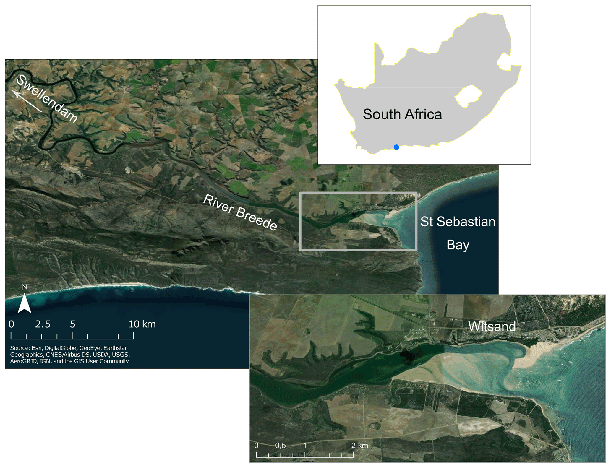
Figure 1Location of the study area and aerial photographs showing the Breede River and the Breede Estuary.
Of South Africa's 291 estuaries, Breede Estuary is one of the largest permanently open estuaries (van Niekerk et al., 2020). Breede River has the fourth largest annual runoff in South Africa (Taljaard, 2003). It flows along 322 km from the south-west of the country in a south-easterly direction towards the South African south coast and enters the Indian Ocean at the town of Witsand in Sebastian Bay (Fig. 1). The estuary extends about 50 km upstream, where the tidal influence ceases (Lamberth et al., 2008).
Breede Estuary is sparsely populated by small settlements of up to 1000 inhabitants (e.g. Witsand; Fig. 1) situated on the northern and southern banks. The estuary provides tourism services with several holiday resorts located along the banks. Numerous farm properties spread along the banks further upstream, and most of the land in the immediate surroundings is privately owned agricultural land (SSI, 2016).
Breede Estuary is open towards the south-east, where it enters the sea against a wave-cut terrace (Carter, 1983). Its mouth is characterized by an open channel, which is located at the southern end of an extensive sand barrier formed by wave action (Schumann, 2013). Over the first 28 km, the depth of the estuary channel ranges from 3–6 m (SSI, 2016). At the lower estuary, the channel meanders along large and shallow sand banks which have formed along the southern shore (Fig. 1).
During the low-flow summer months, the estuary is marine dominated, meaning the estuary receives high seawater input (SSI, 2016). Due to the relatively strong tidal inflow during summer (Taljaard, 2003) and the sand barrier restricting the estuarine inlet, the estuary can be classified as tide and wave dominated (Cooper, 2001).
The main tidal signal is semi-diurnal (M2), with additional diurnal oscillations (Schumann, 2013). During spring tidal periods, the tidal range can reach up to 2 m, as measured at the tide gauge of Witsand, situated at the northern shore of Breede Estuary (Fig. 1). The southern coastline is wave dominated and experiences the highest wave conditions along the entire South African coast (Theron et al., 2010). Thus, waves cause the largest relevant contribution to extreme WLs in South Africa (Melet et al., 2018). Such wave conditions are generated mainly by two synoptic weather systems, namely cold front systems and cut-off lows (Mather and Stretch, 2012). These are responsible for long-period to local swell conditions, with waves approaching the south coast from south-westerly directions. Generally, annual mean significant wave heights (Hs) range from 2.4–2.7 m (Basson et al., 2017). During extreme storm events significant wave heights can reach more than 10 m, and peak periods (Tp) range from 5–20 s. The estuary mouth is relatively sheltered from south-westerly waves since it is protected by a southern headland of the bay (Fig. 1). Waves from the south-eastern sector occur as well; however, these are generated by tropical cyclones, making landfall at the Mozambican and the South African east coast (DEA&DP, 2012). The dominating wind direction is from the westerly and easterly sector, whereby easterly winds generate local wind waves penetrating into the estuary as its opening faces east (Vonkeman et al., 2019). One example of coastal flooding occurring in the area was an extreme storm in August 2008. Waves of 10.7 m were measured, and since the storm lasted longer than 12 h, the extreme waves additionally co-occurred with high tide levels 1 d after a spring tide. Consequently, a large area of the South African south coast was affected, resulting in severe damage to coastal infrastructure (Guastella and Rossouw, 2012).
Table 1Datasets and characteristics applied to set up Delft3D.
a Mean sea level (MSL); b Kaiser et al. (2011), Jung et al. (2011), Wamsley et al. (2009), Mourato et al. (2017), Chow (1959).
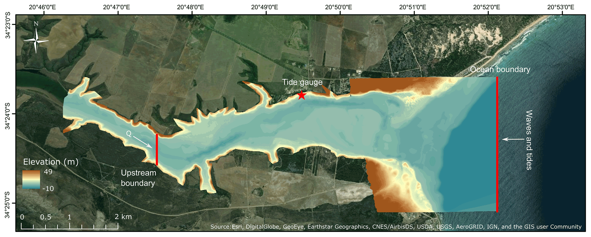
Figure 2Model domain, including the merged bathymetry and elevation raster, the location of the Witsand tide gauge, and the two open boundaries.
During winter, the estuary is highly responsive to freshwater inflows (Taljaard, 2003). The catchment receives 80 % of the annual rainfall during winter months, causing peak flows and floods usually during that season. Breede Estuary has experienced extreme fluvial flooding, with major events occurring in 1906, 2003 and 2008. In November 2008, intense rainfall far upstream, caused by a cut-off low, resulted in extreme river runoff (Holloway et al., 2010). Extreme river discharge caused WLs up to 10 m in the upper 20 km of the estuary while levels of 50 cm were measured at the estuary entrance (Basson et al., 2017). A similar cut-off low event occurred in May 2021 but was less extreme, with estimated elevated WLs being 1–2 m in the upper reaches.
3.1 Hydrodynamic model and data description
We used the fully integrated open-source modelling suite Delft3D (Lesser et al., 2004) which has been extensively used in coastal applications (Lyddon et al., 2018; Bastidas et al., 2016; Kumbier et al., 2018) for simulating flood extents and flood depths from waves, tides, and river discharge, hereafter referred to as Q. We used the hydrodynamic numerical module Delft3D-FLOW, coupled with the module Delft3D-WAVE, which is based on the SWAN (Simulate Waves Nearshore) model.
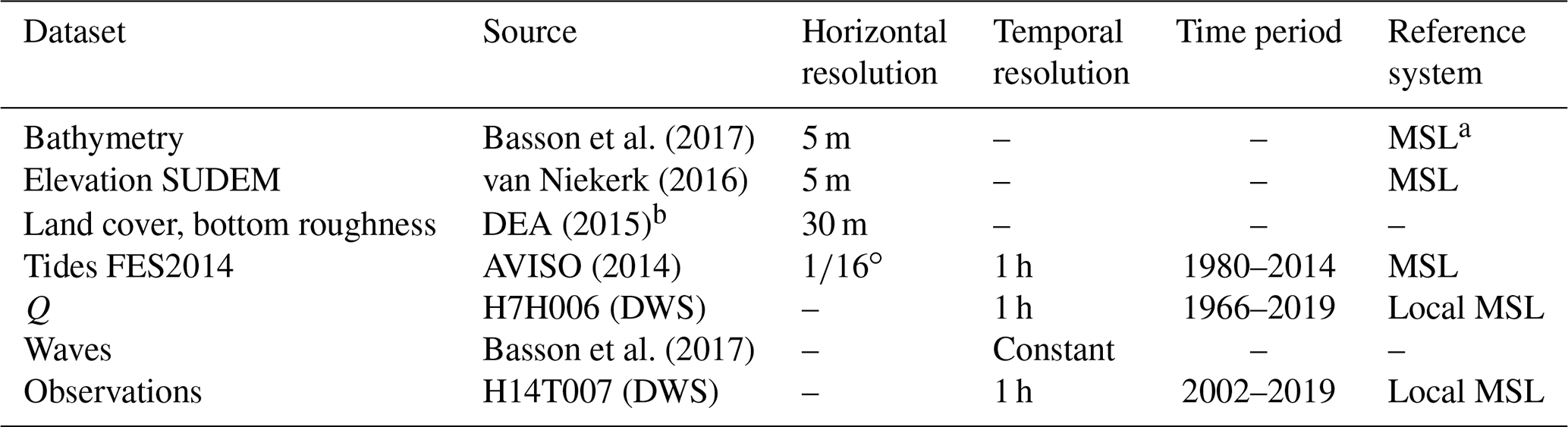
Setting up a hydrodynamic model requires numerous input datasets. The characteristics of the datasets used in this study are shown in Table 1. A detailed description of the pre-processing of the datasets used as Delft3D input files and the model set-up is provided in Appendix A.
Table 2Tidal events used for validation and dates of occurrence.
We performed simulations using tides and Q as input data in Delft3D-FLOW on a 5 m × 5 m rectangular grid in a depth-averaged (2D) mode for the model validation, as well as scenario runs. The 2D mode has been successfully applied in numerous hydrodynamic flood modelling studies (Kumbier et al., 2018; Skinner et al., 2015; Olbert et al., 2017). As we focus on the additional contribution of waves during compound flooding, the model domain is restricted to the lower estuary (Fig. 2). Topographic input data were merged with bathymetric data, which were manually digitized, based on a bathymetry of an existing study report on flood lines at the Breede Estuary (Basson et al., 2017). We specified spatially varying manning bottom roughness via literature review from gridded land cover data (Table 1). We obtained 17 years of hourly measured WL observations serving for the model calibration and validation from the tide gauge station H14T007 (DWS, 2020a), located in the small harbour of the town of Witsand (Fig. 2).
We forced the model at two open boundaries. The ocean boundary (Fig. 2) is located at the westernmost edge of the model domain and perpendicular to the main flow direction. Depending on the scenario, we forced this open boundary with tides and waves. We used historical tidal input data (Table 1) which were obtained from the global tidal FES2014 model (AVISO, 2014; Carrère et al., 2015). The data were extracted at a point closest to but still located 24 km offshore from the westernmost edge of the model domain (Fig. 2). The second boundary (upstream boundary; Fig. 2) is situated at the upstream border of the model domain, perpendicular to the river flow, and was forced by hourly measured Q from the station in Swellendam (Table 1), which was the closest to the upstream boundary (54 km). For the Delft3D-WAVE set-up, we increased the grid cell size and the horizontal resolution of the input bathymetry to 10 m for computational reasons. Since nearshore wave time series could not be obtained, a constant sea state (constant Hs and constant Tp) serves as wave boundary conditions (ocean boundary; Fig. 2) which we obtained from two extreme value analyses (EVAs) performed by Basson et al. (2017).
3.2 Model calibration and validation
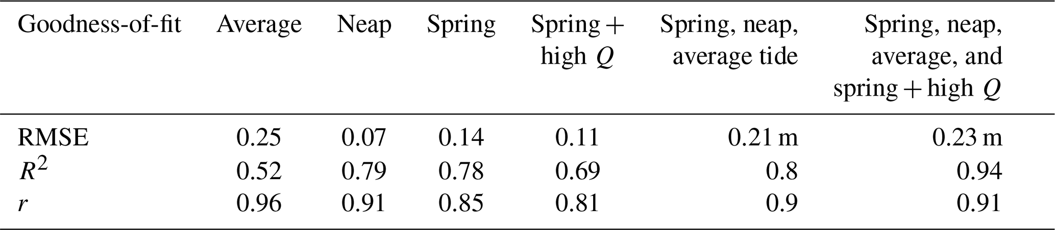
To evaluate the performance of the model, we calculated the goodness-of-fit parameters R2 (coefficient of determination), the Pearson correlation, r, and the root mean square error (RMSE) between the model output and observed WL time series (see Skinner et al., 2015). During model calibration, we adjusted the bottom roughness and horizontal eddy viscosity (see Appendix A). We used the best-fitting physical parameters to set up the model for model validation and the scenario runs. Waves were excluded during model calibration and validation since no measured nearshore wave time series could be obtained.
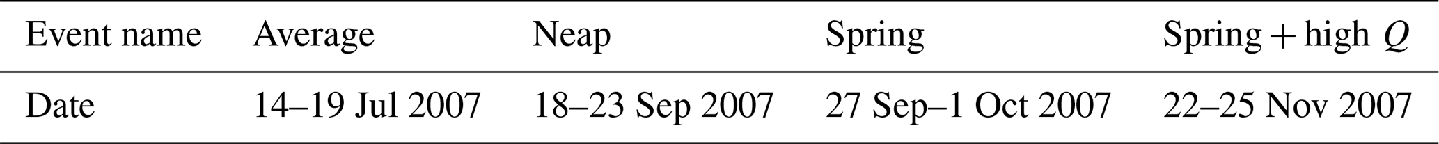
For the validation, we performed three simulations covering the full tidal range and compared the model output to the corresponding observed WLs (Matte et al., 2017; Muis et al., 2017). To account for the full tidal range, these simulations include a spring, average, and a neap tide event (see Table 3 for the event names and dates of occurrence). For these simulations we selected events in which Q was constantly low in order to focus on model performance when the model is driven only from the ocean boundary and where continuous observations exist. To test the performance of the model when driven by both the oceanic and the upstream river boundary, we selected the largest continuously recorded high Q event occurring within the period of observed WLs at the tide gauge in Witsand (Table 2).
According to the tide gauge data, this high Q event (1262.78 m3 s−1) occurred simultaneously with a relatively large tidal range of up to 1.6 m. For this event the time lag of Q reaching the upstream open boundary from the measuring station must be considered. Thus, we estimated the difference between the timing of the peak from the upstream flow gauge and from the non-tidal residual (NTR; see Appendix C) of the tide gauge, whereby we considered the maximum WL as the peak, caused by Q, since the tidal phase at this stage was at low tide level. We estimated a time lag of 8 h, with the peak at the tide gauge occurring later (Fig. D3). We accounted for this time lag in the Q boundary conditions for the validation run to enable the comparison of model output and tide gauge data.
3.3 Event selection and scenario development
To assess compound flooding in terms of magnitude and timing, we developed four scenarios, accounting for tides, waves, and Q. Storm surge was not considered as no nearshore WL time series could be obtained, and offshore input data would even increase model uncertainties. Additionally, analysis of tide gauge data along the South African coastline has shown that at the South African south coast storm surge makes a small contribution, relative to the other considered flood drivers, even when considering extreme surges such as a 100-year event (Theron and Rossouw, 2008; Theron et al., 2014). Moreover, Melet et al. (2018) showed that the wave contribution to extreme WLs in South Africa is substantially larger compared to the surge contribution. To explore this further, we additionally estimated the NTR of the tide gauge data of Witsand, which showed that the mean amplitude of the NTR of 10 cm is small compared to the tidal range of 2 m (Fig. D1). The contribution of wave set-up and Q is still included in the NTR, and large peaks could be identified as being caused by Q (see Fig. D2 and more information on the analysis in Appendix D). To investigate the effects of Q and waves on the flood characteristics during compound flooding, we developed the following scenarios (Table 3).
The scenarios were named according to their driving mechanisms. Thereby T stands for tides, W for waves, and Q for river discharge. The selected extremes were extracted either via peak-over-threshold (POT) analysis or by finding the maxima in the time series. All scenarios assume that the peaks of the drivers occur at the same time (Harrison et al., 2021). The maximum Q event within the hourly time series applied for this study has a peak value of 1357 m3 s−1 and occurred in November 2008. According to Basson et al. (2017) this value was corrected to 1546 m3 s−1, corresponding to a return period of 15 years. The value was corrected as for this event the flow gauging station stopped measuring before the peak was reached. Based on this value, a peak Q of 3295 m3 s−1 corresponds to a 100-year event which we selected here as extreme Q (see Basson et al., 2017, for a more detailed description). We developed the Q hydrograph to force the upstream open boundary by normalizing the hydrograph of the highest Q event for which the full hydrograph was available. We then multiplied the normalized hydrograph with the 100-year peak value. For the STW, so the no-Q scenario, we kept the upstream boundary open so that incoming flood water does not accumulate there. Thus, we chose the lowest measured Q event from the time series, where Q does not exceed 1.2 m3 s−1. For the spring tide event, we selected the maximum tidal flood peak of 1.3 m from the FES2014 tidal input data, which occurred in March 2007.
For the wave conditions, we chose two 100-year wave events from two different extreme value analyses (EVAs) of Basson et al. (2017). According to their EVA, a 100-year wave event coming from east-south-easterly (ESE) directions (110∘), the direction from which waves directly penetrate the estuary, has an Hs of 6.2 m and a Tp of 12 s. To consider an even higher wave event for a final worst-case scenario, Hs was increased to 9.3 m and Tp to 19.95 s, corresponding to Hs and Tp of a 100-year wave event when considering all wave directions in the EVA. The ESE wave direction was maintained for all scenarios that include waves. For the sea states driving the model, it must be pointed out that Basson et al. (2017) performed EVAs on offshore wave data. As the location of the open boundary for this study is located nearshore, the considered wave scenarios may be more extreme than the sea state would be at the open boundary as wave refraction and diffraction were not accounted for. Due to computational constraints and data limitations, we have employed the 100-year return period for waves and Q as this was also recommended by previous flood assessment studies for South Africa (e.g. Theron and Rossouw, 2008; Basson et al., 2017). To compare the results of the WL scenarios, flood extents and flood depths were extracted at the time of the maximum flood.
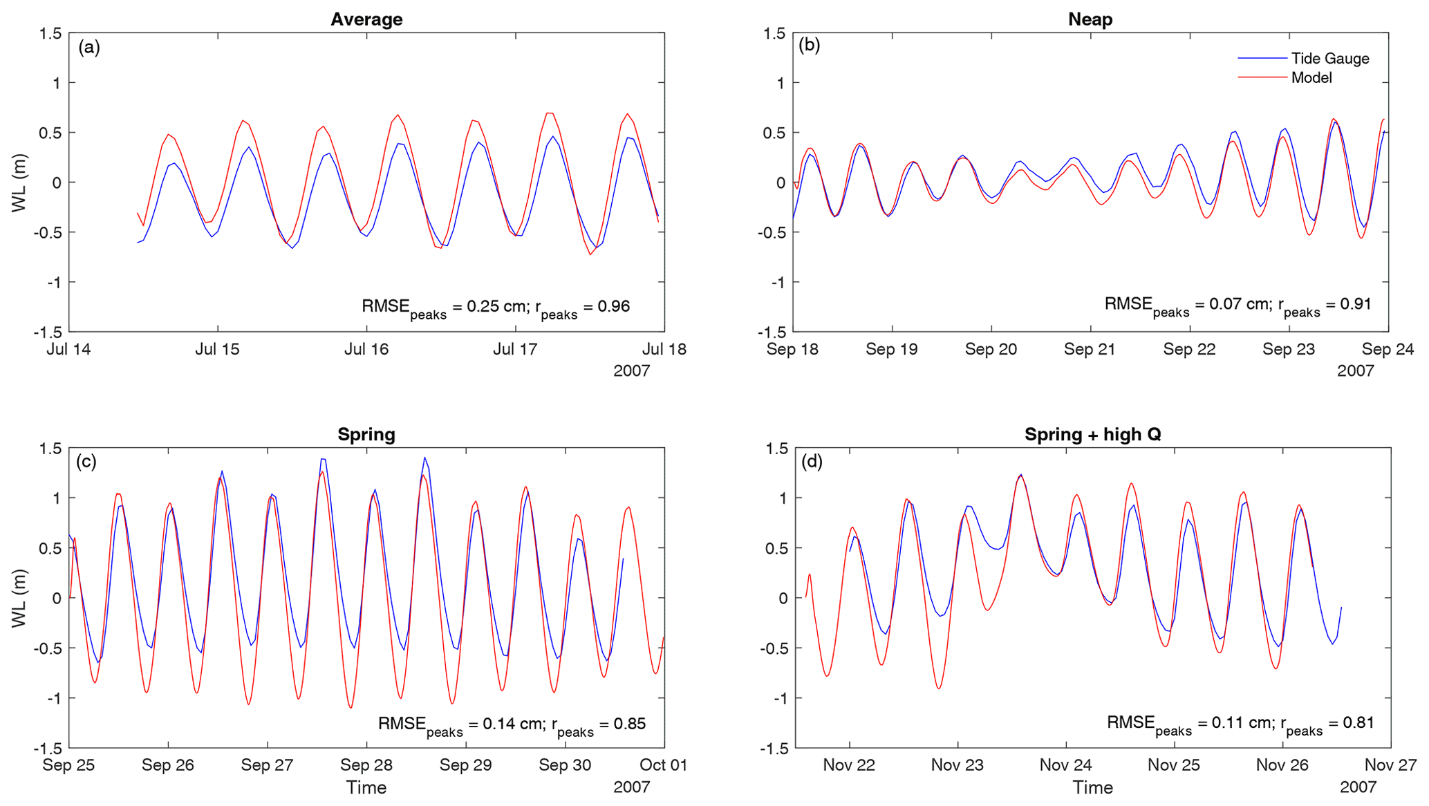
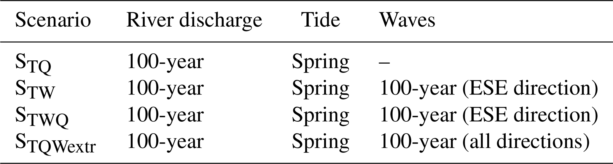
Figure 3WLs of the model validation runs (red curve) at the tide gauge station compared to observed WLs from the tide gauge (blue curve). Panel (a) shows WLs of the average tide event, (b) the neap tide event, (c) the spring tide event, and (d) the high river discharge event, coinciding with the spring high tide. All panels include goodness-of-fit estimates for peak values of each event (RMSEpeaks, rpeaks).
4.1 Model validation
For all validation runs the model set-up was able to reproduce the timing of flood and ebb tide (Fig. 3). Variations occurred however in the WL magnitude, especially during the average event at high tide (Fig. 3a), where simulated WLs were 25 cm higher than the observed for average tidal conditions. During low tide events in the spring tide simulation, modelled WLs were up to 60 cm lower (Fig. 3c), and peak values only, however, showed differences of maximum 14 cm (see RMSE Table C1). The neap tide event on the other hand was simulated with a RMSE of only 10 cm (Fig. 3b) and peak values of only 7 cm (Table C1). The goodness-of-fit estimates also showed agreement of observed and modelled WLs for all tidal events excluding Q (Table C1).
Moreover, for the simulation that included high Q (Fig. 3d) the compared maximum WL peak did not show any difference. After the maximum event peak, however, the model overestimated flood peaks by up to about 30 cm. WLs during low tide before the peak of the event were strongly underestimated (∼ 70 cm) by the model. The goodness of fit, however, did not differ much from tide-only conditions (Table C1). As flooding is usually caused by peak WLs and simulated peaks showed an RMSE of 0.15 m compared to observations for all validation runs, we considered the model performance as fit for purpose.
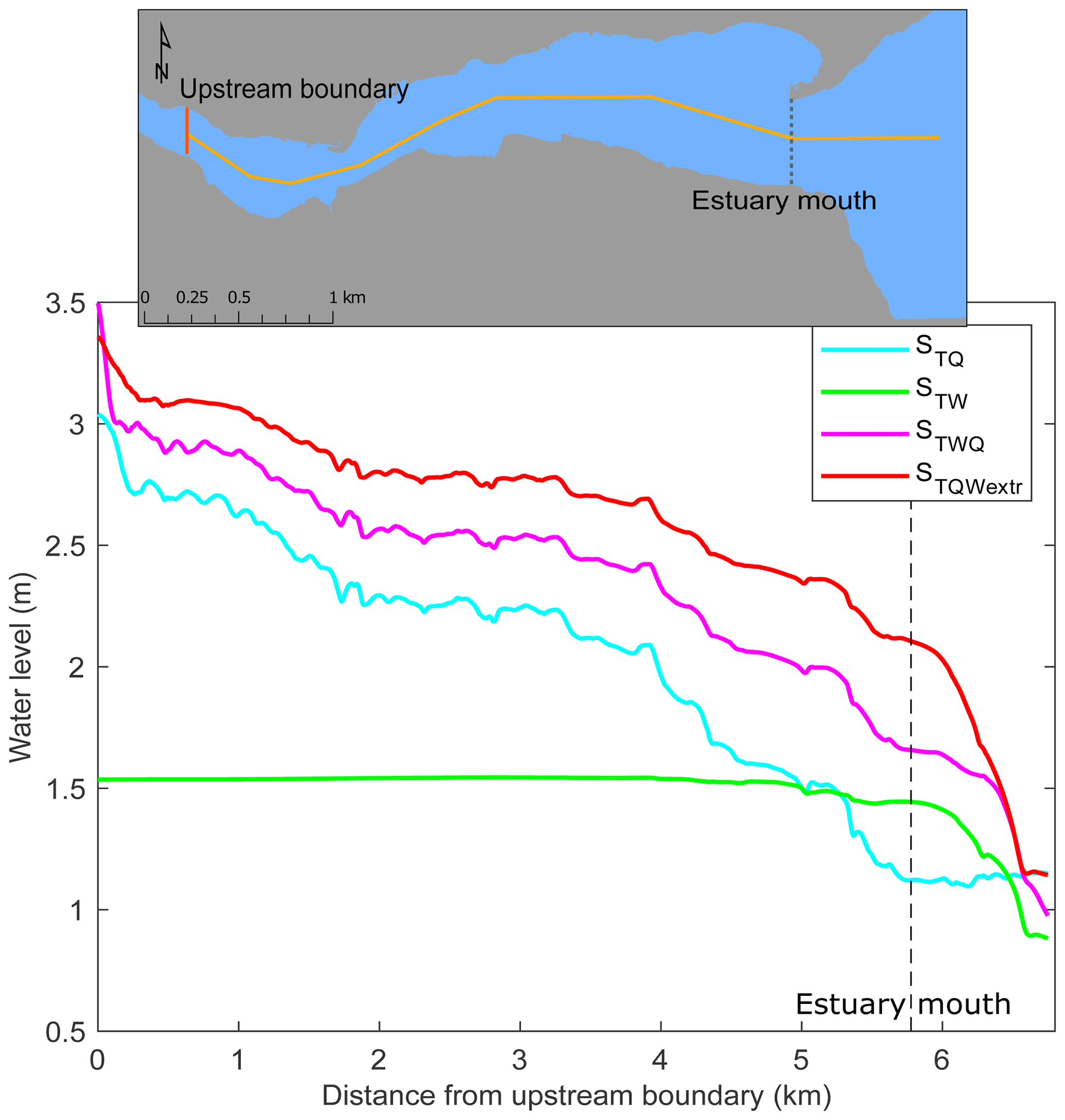
Figure 4WL (m) with distance from the upstream boundary of all scenarios, with the vertical dashed line demonstrating the location of the estuary mouth. The map shows the location of the transect (yellow line), as well as the location of the upstream open boundary (vertical orange line) and the estuary mouth (dashed grey line).
Figure 5Comparison of flood extents of compound scenario and that excluding the driver (a–c) and differences in flood depths (d–f). Panel (d) shows the flood depths of STWQ-STW, (e) shows STWQ-STQ, and (f) shows STQWextr-STWQ.
4.2 Flood sensitivity to varying driver combinations
To analyse the scenario results according to their flood characteristics in terms of magnitude and timing and to estimate the wave contribution, we initially compared the compound flood scenario STWQ to scenarios in which one driver was excluded (STW, STQ). Then we compared the compound flood scenario STWQ with the extreme wave compound flood scenario (STQWextr). WLs, flood extent, and maximum and mean flood depths of all compound scenarios are summarized in Table E1 of Appendix E. For demonstrative reasons we separated the model domain into three areas, termed “upper”, “centre”, and “lower” domains, as shown in Fig. 5.
The results of the compound flood simulation (STWQ) with the simulation excluding river discharge (STW) showed large differences in all flood characteristics. The WLs of STWQ were substantially higher throughout the entire estuary than the WLs produced by accounting only for oceanic drivers (STW; Fig. 4). The WLs of STW showed a continuous state around 1.54 m throughout the entire estuary, slightly decreasing towards the estuary mouth. As in STWQ, WLs were highest at the upstream open boundary and decreased substantially towards the estuary mouth, and the largest WL differences between both scenarios occurred at the upper domain with up to 1.5 m. Further towards the estuary mouth differences reached a minimum of 15 cm, decreasing towards the outside area.
Figure 5a presents the flood extent of STW on top of the extent of STWQ, which showed a substantially larger extent. Further, both scenarios showed large spatial differences in flood extent patterns. STWQ inundated an additional extent of 45 % compared to the flood produced by the STW scenario (Table D1). During the compound scenario, the flood covered a large low-lying area at the northern shore (about 5 km from the mouth), inundating up to 570 m further inland. However, in the scenario STW in which Q was excluded, only a narrow area got flooded, reaching at its widest part 250 m inland. On the southern bank (centre), the STWQ flood reached 80 m further inland than STW. At the estuary mouth, both scenarios flooded about the same areas.
Figure 5b represents differences in flood depths. From the estuary mouth towards the estuary entrance, differences in flood depths showed the same pattern as differences in WLs. At the sand barrier, flood depth differences reached up to 1 m.
Comparing WLs of the Q scenario in which waves were excluded (STQ) to the compound flood scenario STWQ (Fig. 4), both WL curves showed the same pattern, with the WLs of STWQ generally being higher than those simulated by STQ. The differences in WLs between both scenarios decreased from the area around the estuary mouth with maximum differences of 53 cm towards the centre of the study area. We found the smallest differences of ∼ 20 cm close to the upstream edge of the model domain where WLs were highest in both scenarios. We observed a similar pattern in flood depth differences (Fig. 5e), showing a maximum of 70 cm at the northern shore of the estuary entrance, decreasing towards the upstream boundary to ∼ 20 cm. Figure 5b shows the overlaying flood extents of both scenarios, where both scenarios inundated mostly the same areas. The flood extent of STWQ covered a 10 % larger area than the flood resulting from STQ (see Table D1 for the flood size). Inside the estuary, the largest differences occurred in the populated area at the southern shore (centre).
As anticipated, both scenarios accounting for all three drivers during an extreme stage (STWQ and STQWextr) showed the highest values in terms of inundation depth and extent. Comparing the compound flood scenario (STWQ), with the one including even higher extreme waves (STQWextr), we found large differences in the WLs throughout the entire study area (Fig. 4).
Inside the estuary, STQWextr produced continuously higher WLs than STWQ, with increasing differences of up to 40 cm towards the estuary entrance. Such differences are further encountered in the flood depth, showing the same magnitude in the entire lower area. Generally, the higher flood depths produced by STQWextr reached towards the upstream open boundary, but the differences were decreasing (Fig. 5f). The flood extent was 12 % larger when considering large waves during compound flooding. Spatially, the larger flood plain in STQWextr was mainly restricted to the southern shore of the central and lower model domain. In these areas, the STQWextr extent expanded up to 40 m further inland than the extent of STWQ. At the northern shore, the only noticeable area which got flooded in STQWextr, but not in STWQ, was the sand barrier forming the estuary mouth. STQWextr almost entirely flooded the sand dune, indicating that it is likely to be eroded during a flood (Fig. 5c).
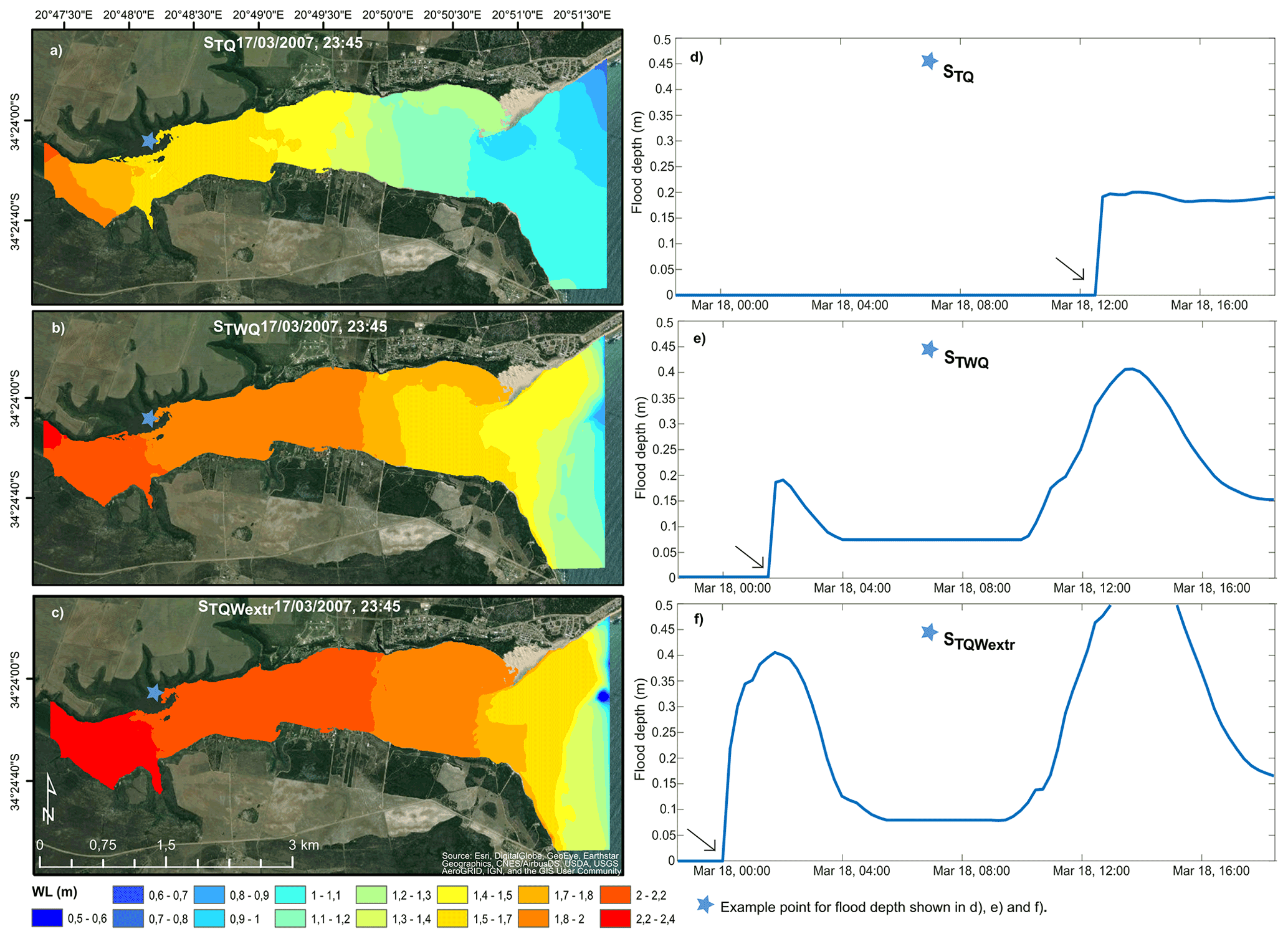
Figure 6WLs of the scenarios STQ, STWQ, and STQWextr, extracted at the same time step (a–c) and time series of all three scenarios (d–f), showing the timing of the onset of the flood extracted from the point marked by the blue star.
To further estimate the effects of waves during compound flooding on the timing of the flood, different time steps of the flood WLs in scenarios STQWextr, STWQ, and STQ are presented in Fig. 6. Figure 6a–c show all three scenarios at the same time step (17 March 2007, 23:45 GMT+2; all times are GMT+2), which was selected according to the onset of high WLs at the upstream open boundary in STQ. The three scenarios at the same time step showed the highest WLs at the upper model domain, which then decreased towards the open sea. Generally, STQ produced the lowest WLs (Fig. 6a), followed by STWQ (Fig. 6b), and the largest WLs were produced in STQWextr (Fig. 6c).
The figure also reveals differences in the areas in which the high WLs dominated at that time. While in STQ WLs of up to 1.8 m were only shown in the upper area, the same magnitude of WLs reached until 4.2 km in STQW and even crossed the estuary mouth in STQWextr. Furthermore, Fig. 6d–f show the timing of the onset of the flood in the three scenarios at the point highlighted by the blue star, shown in Fig. 6a–c. In STQWextr the area got flooded earliest (18 March at 00:00; Fig. 6f) and was followed 90 min later by STQW (Fig. 6e). In STQ, however, the same area got flooded even 12 h later on 18 March at 12:00.
5.1 Effects of interaction between drivers during compound flooding and the contribution of extreme waves
Model outputs show differences in the magnitude of and spatial variation in flood characteristics between all scenarios. Spatial variations in flood characteristics of the different scenarios indicate locations where the interaction of waves, tides, and Q during compound flooding have amplified flooding and where individual drivers contribute to the flood. Enhanced flood characteristics during compound flooding and spatial variations in the flood pattern caused by different driver combinations were previously discussed by Olbert et al. (2017), Kumbier et al. (2018), and Harrison et al. (2021), as well as by Bilskie and Hagen (2018). Yet, none of the studies accounted for the additional influence of waves. In addition to this, none of them addressed the effects of the oceanic flood drivers on the timing of the flood when co-occurring with Q.
The comparison of STWQ with the riverine (STQ) and the wave scenario (STW) highlights that compound flooding increases flood extent and depth. In particular, the additional extent in the central study area, as well as the continuously higher WLs and water depths during compound flooding (Fig. 5a–d), indicates an accumulation of water inside the estuary.
The results further reveal where each driver has its highest influence. This information is relevant for understanding the flood dynamics due to driver interaction and the wave contribution. Regions only inundated in the compound flood scenario but not in STW or STQ were mostly located in the central zone of the study area. In STWQ additional inundated areas in the upper sector were small (10 %) when compared to STQ but were large (45 %) when compared to STW. These floods highlight the generally higher effect of river discharge in the more confined upper section during compound flooding. The influence of Q decreases towards the mouth area as increased friction through the widening of the estuary at the central area and the large flood plain at the upper northern shore of the domain attenuate the flood wave (Cai et al., 2016). In contrast, waves have clearly been shown to be the dominating factor at the estuary mouth area, resulting in substantially higher WLs (Fig. 4). These can be caused by wave set-up as the steep bathymetry and shallow water depths outside the estuary cause waves to break before entering (Carter, 1983; Xu et al., 2020), increasing WLs inside the estuary. Tanaka et al. (2009) have shown that in a shallow and narrow estuary entrance, wave set-up can be up to 14 % of the offshore wave height, which strongly depends on the morphology of the inlet. Olabarrieta et al. (2011) demonstrated that wave set-up propagates inside the estuary and interacts with outflowing currents (Olabarrieta et al., 2011; Zaki et al., 2015). Additionally, the funnelling effect due to the narrow estuary mouth may amplify wave-set-up-induced WLs (Lyddon et al., 2018), contributing to the elevated WLs inside the estuary and causing a relatively large flood extent at the sand barrier in STW. The small differences in flood characteristics in the upper area (STWQ vs. STQ), however, demonstrate a decreasing influence of waves from the entrance towards the upstream boundary of the model domain.
In STWQ the increased WLs at the entrance and the larger flood extents at the sand barrier and in the central estuary indicate an interaction of drivers mostly in the lower area. Delpey et al. (2014) have shown that extreme waves can reduce the freshwater outflow from the estuary mouth towards the open ocean, increasing the water volume inside the estuary, and thereby raise the WLs. Such a blocking of the riverine component through the oceanic component was also observed in Orton et al. (2020), although they only accounted for tides and excluded waves. Hence, the blocking of Q through waves may explain the larger flood characteristics in STWQ at the central domain area, even approximating the upstream open-model boundary. This shows a large contribution of waves to flood characteristics during compound flooding, which was not apparent when considering the components individually. High outflowing Q can also dampen the wave and tidal propagation inside the estuary, causing increased WLs at the entrance (Sassi and Hoitink, 2013). This implies that during compound flooding, waves play a stronger role when coinciding with Q by amplifying the flood magnitude. When considering flood drivers individually, however, the effects caused by waves were relatively low, as compared to effects caused by Q.
We further assessed the wave contribution by testing the sensitivity of compound flooding to more extreme wave conditions. Comparing results of the compound flood scenario STWQ with results of the extreme wave compound flood (STQWextr) confirms the expected larger flooding caused by more intense waves. This was valid for all flood characteristics throughout the entire study area. The effects of increased wave conditions were found to be greatest in the lower reaches. First, the considerably larger flood extent at the sand barrier can be explained by wave overtopping and shows that extreme wave conditions coinciding with spring high tides may lead to eroding and a breaching of the barrier. As explained above, wave set-up can raise WLs inside the estuary (Olabarrieta et al., 2011), which becomes more extreme with higher waves. An impact of waves on WL variabilities in South African estuaries has previously been shown by Schumann (2013) who states that waves together with the tidal influence can determine how far ocean water propagates upstream in an estuary. Therefore, increased wave conditions during compound flooding do not only have effects on the lower domain flood extent and depth. STQWextr-enhanced flood characteristics in the upper domain, as shown in all STQWextr-related figures (Figs. 4, 5c and f, and 6c and f), confirm the fact that higher waves cause greater impacts further upstream when compared to STWQ.
Last, an interesting finding of the study is that compound events do not only affect flood characteristics in terms of magnitude.
The timing of the flood also changed when all drivers coincide and when stronger wave conditions are accounted for. The increased volumes of water during the compound event and in STQWextr resulted in flooding occurring earlier than when the drivers, waves, and Q were not coinciding. Figure 6 shows that at the specific considered time step, the flood characteristics of STQWextr were largest (also in the upper area), although at that time Q was still moderate. Therefore, even when the riverine component was still moderate, waves led to enhanced flooding. Considering the timing at which most of the flood plain marked in Fig. 6 was inundated in all three scenarios (see Fig. 6d–f) further highlights the large wave contribution during compound flooding. In this case the flood plain was flooded earliest in STQWextr, followed by STWQ about 95 min later. When not accounting for waves, however, the flood plain was inundated 12 h later than in STWQ. These findings indicate that waves play a substantial role when coinciding with the fluvial component and spring tides as they lead to larger flooding and an earlier onset of the inundation, even when Q was still moderate.
5.2 Model performance, limitations, and outlook
This analysis has shown the sensitivity of flood characteristics to compound flooding when compared to individual flood drivers. This was demonstrated by spatial variabilities in the flood extents and by variabilities in the flood magnitude and timing. We must note, however, that flood extent and depths could not be directly validated. Commonly used data types for flood impact validation are pictures, satellite imagery, and high watermarks (Molinari et al., 2017). Yet, such data were not available for the study area. According to Basson et al. (2017), pictures and high watermarks of a fluvial flood occurring in 2008 exist, however, only at sites further upstream. This area was not considered in the model domain of this study as detailed upstream bathymetry data could not be obtained. Nevertheless, model performance was validated at the tide gauge at Witsand near the mouth (Fig. 2). Flood peaks matched the observed peaks in almost all simulations (Fig. 3, Table C1). The model overestimated tidal high-water peaks only during the average tide event. Tidal low water peaks, though, were generally underestimated.
Those differences can be explained by uncertainties inherent in the model input data, such as tides and bathymetry. Tides, serving as input data for model validation and all scenarios of this study, were obtained from the global FES2014 tidal model (Carrère et al., 2015). Even though the model shows a rather high accuracy offshore, on shelves, and on nearshore areas (Stammer et al., 2014; Ray et al., 2019), the local-scale coastal processes caused by the local topography and the influence of the estuarine channel morphology (Wang et al., 2019; Godin and Martínez, 1994) are not considered in the data. Additionally, the model open boundary was placed at a location several kilometres further nearshore of the point from which the tidal inputs were extracted. Processes modifying the tidal propagation between both locations were therefore not considered. One way to overcome this limitation would be to downscale the tides from the model towards the location of the open boundary, which, however, is beyond the scope of this study. Moreover, permanently opened estuaries are highly dynamic areas due to a constant influence of sediment deposition by river inflow and sediment removal due to floods (Moore et al., 2009; Whitfield et al., 2012). The sand bars and sand banks at the timing of the validation runs (covering events in 2007) were therefore likely in a different position than at the time when the input bathymetry was generated (Basson et el., 2017). This can have a high impact on water levels at the location of the tide gauge (Wang et al., 2019). Additionally, the omitted storm surge, wind, and waves as model input during the validation runs can explain the large discrepancies occurring specifically in the Q validation run (Fig. 3d), in which tidal low water peaks preceding the actual event peak were strongly underestimated in the model. Thus, the higher observed WLs could have been produced by wave set-up or less likely a storm surge (Zaki et al., 2015). Relative to other flood drivers, storm surge alone does not have a significant effect on coastal flooding along the South African south and west coasts (Theron et al., 2014), but it still may affect WLs inside the estuary (Lyddon et al., 2018). Testing the effect of waves and surge on the model performance, however, would require observed wave time series and nearshore WL data which were not available for this study.
Storm surge has been considered in most regional or local flood assessments, specifically in those dealing with compound flooding (Eilander et al., 2020; Olbert et al., 2017; Shen et al., 2019). Despite its low contribution at the location of Breede Estuary (Appendix C), storm surge may still contribute to compounding drivers to become an extreme event, even when neither of the drivers is extreme (Leonard et al., 2014). To estimate its contribution, storm surge should be considered in further simulations. Our analysis presents driver interactions during extreme (100-year) conditions without showing joint probabilities of waves and Q. Further, we assumed that maximum flooding occurs when all drivers peak simultaneously and did not account for differences in the relative timing of all driver peaks. However, Harrison et al. (2021) conducted such a sensitivity analysis and found that the effect of the timing of driver peaks strongly depended on estuary size. They also found that in an estuary comparable in size to Breede Estuary this effect was negligible. However, as estuaries can also differ in aspects other than size (e.g. morphological characteristics), assessing the effect of the timing of the driver peaks could provide further insights on the flood mechanisms of compound flooding. This information, together with information on joint probabilities, becomes relevant when assessing risk from compound flooding, which is beyond the scope of this study and should be considered in future work. For such a risk assessment a wider range of return periods should also be explored.
We assessed compound flooding from tides, Q, and waves at the permanently open Breede Estuary (South Africa) using a hydrodynamic model. For the assessment, we simulated scenarios accounting for the three flood drivers (i.e. tides, Q, and waves) and scenarios omitting either waves or Q in order to analyse their contribution. We found that flood characteristics such as extent, water depth, and timing are affected by the interaction between the drivers. As anticipated, the omission of waves caused major inundations to occur in the upper domain area, whereas the omission of Q produced comparably small flooding. Thus, we have shown that when considered separately, the contribution of waves to flooding was small. When waves were combined with spring tides and Q, however, they had a substantial effect on the spatial distribution and magnitude of the floods by impeding river flow to the sea. A notable impact of waves during compound flooding was their effect on the flood timing. Through backwater effects, waves induced the flood to occur earlier. This was further emphasized when increasing the wave intensity in the compound flood scenario. We therefore suggest that compound flooding induced by high Q, tides, and waves should not only be considered in risk assessment studies in terms of magnitude but also in terms of timing. The earlier onset of intense flooding needs to be accounted for when forecasting, planning, and managing flood hazards.
As we have shown in this study for Breede Estuary, compound flooding can exacerbate flooding, and waves make a substantial contribution to flooding when coinciding with extreme Q. Extreme waves co-occurring with spring tides and high precipitation have been documented by Guastella and Rossouw (2012), who additionally predicted a change in wave climate for the South African south-west coast towards more frequent extreme wave conditions. Our results in combination with a changing wave climate further confirm the necessity of accounting for compound flooding and specifically waves in future local flood impact assessments in South Africa, particularly for other South African estuaries, which are highly populated, like Umgeni Estuary (Durban), Swartkops Estuary (Port Elizabeth), Nahoon Estuary (East London), and Diep Estuary (Cape Town), where it can lead to substantial infrastructure damage. The achievement of data for complex modelling studies, as well as validating model results, in South Africa remains a major challenge, however.
For the hydrodynamic model we used the 5 m SUDEM elevation dataset (van Niekerk, 2016) merged with bathymetric data, which we manually digitized, based on a bathymetry of a study report on flood lines at the Breede Estuary (Basson et al., 2017). As model friction parameters, we specified spatially varying manning values from land cover raster data, provided by the Department of Environmental Affairs (DEA, 2015), originally coming in a 30 m horizontal resolution. Manning roughness values for the different land cover classes were derived from a literature review, following Kaiser et al. (2011), Jung et al. (2011), Wamsley et al. (2009), Mourato et al. (2017), and Chow (1959).
As model boundary conditions we used historical tidal input data, which we obtained from the global tidal FES2014 model (AVISO, 2014; Carrère et al., 2015). We extracted the data at a point closest to but still located 24 km offshore from the open boundary. The time series covers a period of 34 years from 1980–2014. We obtained hourly measured river discharge from the station H7H006 in Swellendam, which was the closest to the upstream boundary (54 km). The data were provided by the Department for Water and Sanitation (DWS) of South Africa (DWS, 2020b) and cover a period of 53 years, from 1966 until 2019. Hourly water level observations serving for the model calibration and validation were provided by the DWS from the tide gauge station H14T007 (DWS, 2020a), located in a small harbour of the town of Witsand inside the estuary mouth. The measurements cover 17 years (2002–2019). We derived wave data, significant wave height (Hs), and peak period (Tp) from two extreme value analyses (EVAs) performed by Basson et al. (2017). They extracted from the ECMWF model simulated offshore wave data of 37 years (1979–2016), from a point close to the estuary, while still being located 30 km off the coast.
Grid and topography of the model are based on the Cartesian coordinate system WGS84/UTM zone 34S. The model domain expands over an area of 19.2 km2, covering the lower estuary and the area until 1.5 km offshore (Fig. 2). We used a time step of 1.5 s for calibration, validation, and scenario runs, as was suggested by the Courant number. We changed the reflection parameter α, which determined the permeability of the open boundaries to 1000 for the ocean boundary and to 200 for the upstream boundary, as the model otherwise produced instabilities in preliminary runs (Deltares, 2014a). Additionally, we considered several physical and numerical parameters for the model set-up. These were either kept at the default value, as suggested by Deltares (2014), or were changed and adjusted during model calibration runs. For the wave set-up we increased the grid cell size to 10 m for computational reasons. We used a JONSWAP (Joint North Sea Wave Project) spectrum with a peak enhancement factor of 1.75 and a wave direction spreading of 30∘ according to Basson et al. (2017).
For the model calibration we selected an event occurring from 26 June until 3 July 2003 due to the low and constant river discharge before, during, and after the calibration event (max 3 m3 s−1). This is important because the time lag of the river discharge between the measuring station in Swellendam and the upstream open boundary of the model domain is not considered. Waves were excluded during model calibration and validation. For the model calibration we changed the physical parameters' bottom roughness and horizontal eddy viscosity, as these can affect the tidal amplitude and the speed of the tidal wave propagation into the estuary (Skinner et al., 2015; Garzon and Ferreira, 2016). Table B1 shows changed physical parameters and goodness of fit estimates, resulting from compared modelled and observed time series. The best-fitting physical parameters resulting from the calibration were used to set up the model for the validation and scenario runs even though the improvements were small (see Table B1).
Table B1Parameter changes during model calibration and final model set-up.

Table C1Goodness-of-fit estimates of model validation runs compared to observations. Columns 2–4 show goodness-of-fit estimates for each tidal event of flood peaks only. Column 5 shows the goodness of fit for tide-only conditions (entire time series) and column 6 for tides including high river discharge (entire time series).
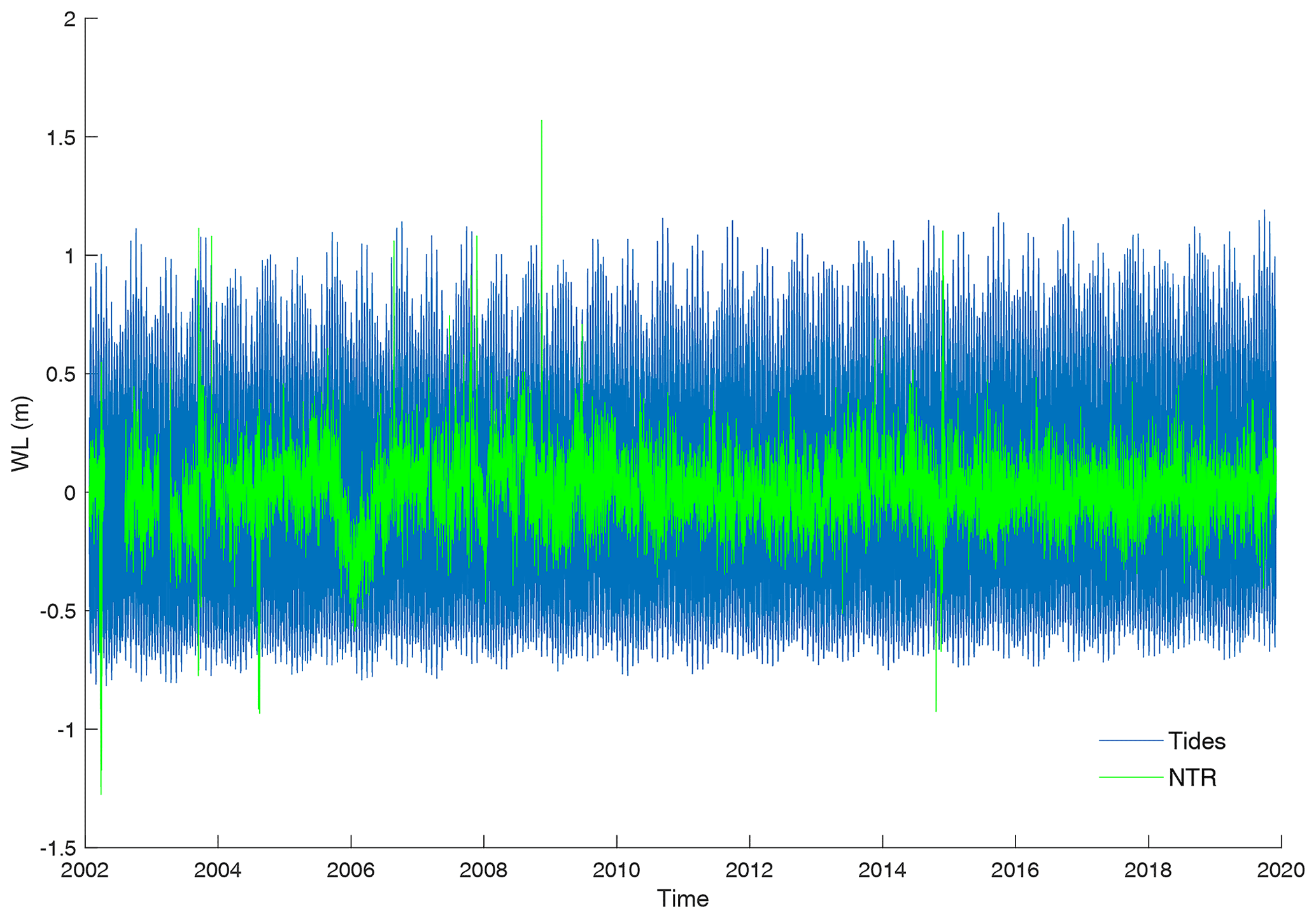
To estimate storm surge height at Breede Estuary, we extracted the non-tidal residual (NTR) of the Witsand tide gauge time series. Then we performed a harmonic analysis on the water levels using the UTide package of Codiga (2011) and subtracted the resulting tidal signal from the tide gauge data. The tidal signal plotted against the NTR is shown in Fig. D1. We calculated the mean amplitude of the entire NTR time series (0.1 m) and the mean peak height of all NTR peaks, including outliers, being 0.54 m. Only several outliers exceed the average peak height of the NTR, reaching up to 1.7 m (Fig. D1). As the NTR still contains the signal of river discharge from Breede River, we tested if peaks can be related to river discharge. Thus, we tested if NTR peaks occurred within 3 d after peaks of river discharge time series measured in Swellendam. In total nine NTR peaks were considered as being caused by high river discharge, of which five are highlighted in Fig. D2, for the period 2007–2010. Additional to river discharge and non-linear interactions, the NTR at Witsand includes wave set-up. The contribution of wave set-up to coastal water levels has already been shown by Dodet et al. (2019). As for our local study no measured nearshore wave time series could be obtained neither for the study area nor for close by locations, and it is difficult to estimate the contribution of wave set-up. In a widely applied formula wave set-up has been estimated to be 0.2× Hs (e.g. Vousdoukas et al., 2016). Like according to Basson et al. (2017) and Guastella and Rossouw (2012), Hs can exceed 10 m (100-year return period) in the area that Breede Estuary is located, and we can, according to the named wave set-up estimations, assume that the component contributes a substantial proportion to the NTR, underlining the assumption of a comparably small surge contribution.
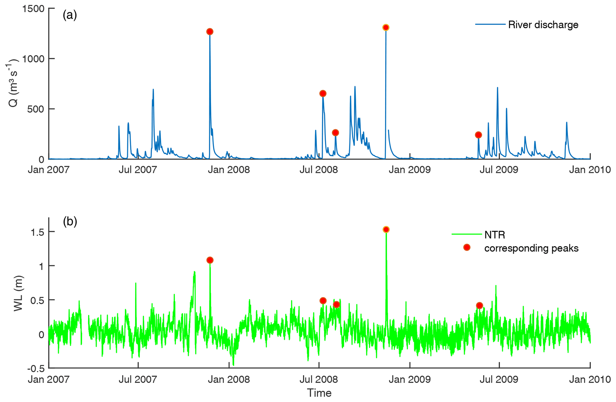
Figure D2River discharge for the period 2007–2010 with peaks (red markers) occurring within 3 d before peaks of NTR (a). NTR at Witsand with peaks (red markers) occurring within 3 d after peaks of river discharge (b). The period 2007–2010 was chosen for representative reasons, as this was the period containing the most peaks.
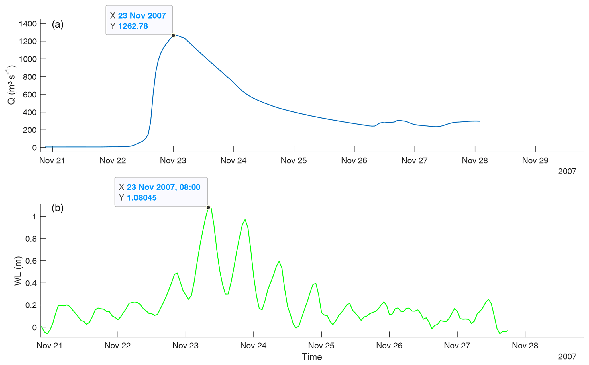
Figure D3Validation event (22–25 November 2007) of river discharge at the flow gauge Swellendam (a) and of the NTR at the tide gauge in Witsand (b); between both peaks we estimated a time lag of 8 h.
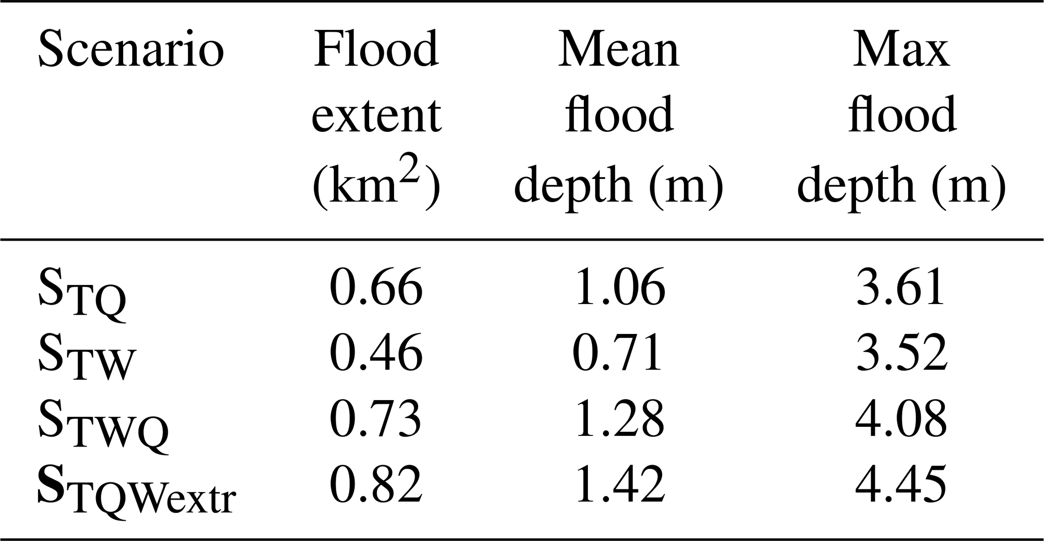
Table E1Flood extents and maximum and mean flood depths of all scenarios.
All data used in this paper are properly cited and referred to in the reference list. The local tide gauge and flow gauge data can be obtained under request from the DWS or can be downloaded from this web page: http://www.dwa.gov.za/hydrology (DWS, 2020a, b). FES2014 global tide model data are publicly available at https://www.aviso.altimetry.fr/es/data/products/auxiliary-products/global-tide-fes.html (AVISO, 2014). The SUDEM can be purchased from Stellenbosch University for research purposes at https://doi.org/10.13140/RG.2.1.3015.5922 (van Niekerk, 2016). Bathymetric data and model output can be provided from the first author on request.
SK defined the research problem, collected the data, performed all the analyses, prepared the figures, and wrote the first draft of the manuscript. SSA provided advice on the methodology, and SSA and AV supervised the work of SK. LN and MLV helped with finding the study area, and LN and MLV provided relevant literature and links to hosted datasets. SSA, AV, MLV, and LN reviewed the manuscript.
The contact author has declared that neither they nor their co-authors have any competing interests.
Publisher's note: Copernicus Publications remains neutral with regard to jurisdictional claims in published maps and institutional affiliations.
This article is part of the special issue “Understanding compound weather and climate events and related impacts (BG/ESD/HESS/NHESS inter-journal SI)”. It is not associated with a conference.
We have received additional financial support for the publication from the state of Schleswig-Holstein within the funding programme Open-Access-Publikationsfonds. Lara van Niekerk and Melanie Lück-Vogel were funded through the Coastal Systems CSIR Parliamentary Grant (PG) from the Department of Science and Innovation (DSI).
This paper was edited by Jakob Zscheischler and reviewed by two anonymous referees.
AVISO: FES2014 – Global tide model: FES2014 was produced by Noveltis, Legos and CLS and distributed by Aviso+, with support from Cnes, AVISO [data set], https://www.aviso.altimetry.fr/es/data/products/auxiliary-products/global-tide-fes.html (last access: 13 November 2020), 2014.
Basson, G., van Zyl, J., Bosman, E., Sawadago, O., and Vonkeman, J.: Conduct a coastal vulnerability: Breede River Estuary Floodline Assessment, Technical Report, DEA&DP, Western Cape, South Africa, 313 pp., 2017.
Bastidas, L. A., Knighton, J., and Kline, S. W.: Parameter sensitivity and uncertainty analysis for a storm surge and wave model, Nat. Hazards Earth Syst. Sci., 16, 2195–2210, https://doi.org/10.5194/nhess-16-2195-2016, 2016.
Bevacqua, E., Maraun, D., Vousdoukas, M. I., Voukouvalas, E., Vrac, M., Mentaschi, L., and Widmann, M.: Higher probability of compound flooding from precipitation and storm surge in Europe under anthropogenic climate change, Science Advances, 5, eaaw5531, https://doi.org/10.1126/sciadv.aaw5531, 2019.
Bilskie, M. V. and Hagen, S. C.: Defining Flood Zone Transitions in Low-Gradient Coastal Regions, Geophys. Res. Lett., 45, 2761–2770, https://doi.org/10.1002/2018GL077524, 2018.
Bilskie, M. V., Zhao, H., Resio, D., Atkinson, J., Cobell, Z., and Hagen, S. C.: Enhancing Flood Hazard Assessments in Coastal Louisiana Through Coupled Hydrologic and Surge Processes, Front. Water, 3, 832, https://doi.org/10.3389/frwa.2021.609231, 2021.
Brown, S., Nicholls, R. J., Goodwin, P., Haigh, I. D., Lincke, D., Vafeidis, A. T., and Hinkel, J.: Quantifying Land and People Exposed to Sea-Level Rise with No Mitigation and 1.5 ∘C and 2.0 ∘C Rise in Global Temperatures to Year 2300, Earths Future, 6, 583–600, https://doi.org/10.1002/2017EF000738, 2018.
Cai, H., Savenije, H. H. G., Jiang, C., Zhao, L., and Yang, Q.: Analytical approach for determining the mean water level profile in an estuary with substantial fresh water discharge, Hydrol. Earth Syst. Sci., 20, 1177–1195, https://doi.org/10.5194/hess-20-1177-2016, 2016.
Carrère, L., Lyard, F., Cancet, M., and Guillot, A.: FES 2014, a new tidal model on the global ocean with enhanced accuracy in shallow seas and in the Arctic region, EGU General Assembly, available at: https://ui.adsabs.harvard.edu/abs/2015EGUGA..17.5481C/abstract (last access: 24 January 2022), 2015.
Carter, R. A.: Report 21 of the Estuaries of the Cape, Part 2: Synopses of available information on individual systems series, CSIR (CSIR research report 420), http://researchspace.csir.co.za/dspace/handle/10204/3462 (last access: 24 January 2022), 1983.
Chen, W.-B. and Liu, W.-C.: Modeling Flood Inundation Induced by River Flow and Storm Surges over a River Basin, Water, 6, 3182–3199, https://doi.org/10.3390/w6103182, 2014.
Chow, V. T.: Open-channel hydraulics, Blackburn Press, Caldwell, NJ, 680 pp., 1959.
Church, J. A., Clark, P. U., Cazenave, A., Gregory, J. M., Jevrejeva, S., Levermann, A., Merrifield, M. A., Milne, G. A., Nerem, R. S., Nunn, P. D., Payne, A. J., Pfeffer, W. T., Stammer, D., and Unnikrishnan, A. S.: Sea Level Change, Cambridge University Press, Cambridge, UK, and New York, NY, USA, 2013.
Codiga, D. L.: Unified tidal analysis and prediction using the UTide Matlab functions, Graduate School of Oceanography, University of Rhode Island, https://doi.org/10.13140/RG.2.1.3761.2008, 2011.
Cooper, J. A. G.: Geomorphological variability among microtidal estuaries from the wave-dominated South African coast, Geomorphology, 40, 99–122, 2001.
Couasnon, A., Eilander, D., Muis, S., Veldkamp, T. I. E., Haigh, I. D., Wahl, T., Winsemius, H. C., and Ward, P. J.: Measuring compound flood potential from river discharge and storm surge extremes at the global scale, Nat. Hazards Earth Syst. Sci., 20, 489–504, https://doi.org/10.5194/nhess-20-489-2020, 2020.
DEA: 2013-14 National Land Cover – 72 classes, Department of Environmental Affairs, https://doi.org/10.15493/DEA.CARBON.10000028, 2015.
DEA&DP: Sea Level Rise and Flood Risk Assessment for a Select Disaster Prone Area Along the Western Cape Coast. Level Rise and Flood Risk Modelling: Phase B: Overberg District Municipality. Phase 2 Report: Overberg District Municipality Sea, Department of Environmental Affairs and Development Planning, https://www.westerncape.gov.za/eadp/files/atoms/files/Overberg DM SLR Phase 3 Risk Assessment Final (March 2012).pdf (last access: 24 January 2022), 2012.
DEFF: National Coastal Climate Change Vulnerability Assessment: Vulnerability Indices – Technical Report, Department of Environment, Forestry and Fisheries, Pretoria, South Africa, 2020.
Delpey, M. T., Ardhuin, F., Otheguy, P., and Jouon, A.: Effects of waves on coastal water dispersion in a small estuarine bay, J. Geophys. Res.-Oceans, 119, 70–86, https://doi.org/10.1002/2013JC009466, 2014.
Deltares: Delft3D-FLOW: Simulation of multidimensional hydrodynamic flows and transport phenomena, including sediments, User Manual, Deltares, available at: https://oss.deltares.nl/documents/183920/185723/Delft3D-FLOW_User_Manual.pdf (last access: 19 July 2021), 2014.
Dodet, G., Melet, A., Ardhuin, F., Bertin, X., Idier, D., and Almar, R.: The Contribution of Wind-Generated Waves to Coastal Sea-Level Changes, Surv. Geophys., 40, 1563–1601, https://doi.org/10.1007/s10712-019-09557-5, 2019.
DWS: Station H14T007, Department of Water and Sanitation, available at: http://www.dwa.gov.za/hydrology (last access: 11 September 2020), 2020a
DWS: Station H7H006, Department of Water and Sanitation, available at: http://www.dwa.gov.za/hydrology (last access: 11 September 2020),, 2020b.
Eilander, D., Couasnon, A., Ikeuchi, H., Muis, S., Yamazaki, D., Winsemius, H., and Ward, P. J.: The effect of surge on riverine flood hazard and impact in deltas globally, Environ. Res. Lett., 15, 104007, https://doi.org/10.1088/1748-9326/ab8ca6, 2020.
Fitchett, J. M., Grant, B., and Hoogendoorn, G.: Climate change threats to two low-lying South African coastal towns: Risks and perceptions, S. Afr. J. Sci, 112, 1–9, https://doi.org/10.17159/sajs.2016/20150262, 2016.
Garzon, J. and Ferreira, C.: Storm Surge Modelling in Large Estuaries: Sensitivity Analyses to Parameters and Physical Processes in the Chesapeake Bay, Journal of Marine Science and Engineering, 4, 45, https://doi.org/10.3390/jmse4030045, 2016.
Godin, G. and Martínez, A.: Numerical experiments to investigate the effects of quadratic friction on the propagation of tides in a channel, Cont. Shelf Res., 14, 723–748, https://doi.org/10.1016/0278-4343(94)90070-1, 1994.
Guastella, L. A. and Rossouw, M.: Coastal vulnerability: What will be the impact of increasing frequency and intensity of coastal storms along the South African coast?, Reef Journal, 2, 129–139, 2012.
Hallegatte, S., Green, C., Nicholls, R. J., and Corfee-Morlot, J.: Future flood losses in major coastal cities, Nat. Clim. Change, 3, 802–806, https://doi.org/10.1038/nclimate1979, 2013.
Hanson, S., Nicholls, R., Ranger, N., Hallegatte, S., Corfee-Morlot, J., Herweijer, C., and Chateau, J.: A global ranking of port cities with high exposure to climate extremes, Climatic Change, 104, 89–111, https://doi.org/10.1007/s10584-010-9977-4, 2011.
Harrison, L. M., Coulthard, T. J., Robins P. E., and Lewis, M. J.: Sensitivity of Estuaries to Compound Flooding, Estuar. Coast., 44, 387, https://doi.org/10.1007/s12237-021-00996-1, 2021.
Hendry, A., Haigh, I. D., Nicholls, R. J., Winter, H., Neal, R., Wahl, T., Joly-Laugel, A., and Darby, S. E.: Assessing the characteristics and drivers of compound flooding events around the UK coast, Hydrol. Earth Syst. Sci., 23, 3117–3139, https://doi.org/10.5194/hess-23-3117-2019, 2019.
Holloway, A., Fortune, G., Chasi, V., and Beckman, T.: RADAR Western Cape 2010: Risk and development annual review, PeriPeri Publications, Disaster Mitigation for Sustainable Livelihoods Programme, Rondebosch, xv, 104, 2010.
Hughes, P. and Brundrit, G. B.: Sea Level Rise and Coastal Planning: A Call for Stricter Control in River Mouths, J. Coastal Res., 11, 887–898, 1995.
IPCC: Climate change 2014: Synthesis report, Contribution of Working Groups I, II and III to the Fifth Assessment Report of the Intergovernmental Panel on Climate Change, Intergovernmental Panel on Climate Change, Geneva, Switzerland, 151 pp., 2014.
Jung, I., Park, J., Park, G., Lee, M., and Kim, S.: A grid-based rainfall-runoff model for flood simulation including paddy fields, Paddy Water Environ., 9, 275–290, 2011.
Kaiser, G., Scheele, L., Kortenhaus, A., Løvholt, F., Römer, H., and Leschka, S.: The influence of land cover roughness on the results of high resolution tsunami inundation modeling, Nat. Hazards Earth Syst. Sci., 11, 2521–2540, https://doi.org/10.5194/nhess-11-2521-2011, 2011.
Kirezci, E., Young, I. R., Ranasinghe, R., Muis, S., Nicholls, R. J., Lincke, D., and Hinkel, J.: Projections of global-scale extreme sea levels and resulting episodic coastal flooding over the 21st Century, Sci. Rep.-UK, 10, 11629, https://doi.org/10.1038/s41598-020-67736-6, 2020.
Klerk, W. J., Winsemius, H. C., van Verseveld, W. J., Bakker, A. M. R., and Diermanse, F. L. M.: The co-incidence of storm surges and extreme discharges within the Rhine–Meuse Delta, Environ. Res. Lett., 10, 35005, https://doi.org/10.1088/1748-9326/10/3/035005, 2015.
Kumbier, K., Carvalho, R. C., Vafeidis, A. T., and Woodroffe, C. D.: Investigating compound flooding in an estuary using hydrodynamic modelling: a case study from the Shoalhaven River, Australia, Nat. Hazards Earth Syst. Sci., 18, 463–477, https://doi.org/10.5194/nhess-18-463-2018, 2018.
Lamberth, S. J., van Niekerk, L., and Hutchings, K.: Comparison of, and the effects of altered freshwater inflow on, fish assemblages of two contrasting South African estuaries: The cool-temperate Olifants and the warm-temperate Breede, Afr. J. Mar. Sci., 30, 311–336, https://doi.org/10.2989/AJMS.2008.30.2.9.559, 2008.
Lee, S., Kang, T., Sun, D., and Park, J.-J.: Enhancing an Analysis Method of Compound Flooding in Coastal Areas by Linking Flow Simulation Models of Coasts and Watershed, Sustainability, 12, 6572, https://doi.org/10.3390/su12166572, 2020.
Leonard, M., Westra, S., Phatak, A., Lambert, M., van den Hurk, B., McInnes, K., Risbey, J., Schuster, S., Jakob, D., and Stafford-Smith, M.: A compound event framework for understanding extreme impacts, WIREs Clim. Change, 5, 113–128, https://doi.org/10.1002/wcc.252, 2014.
Lesser, G. R., Roelvink, J. A., van Kester, J. A. T. M., and Stelling, G. S.: Development and validation of a three-dimensional morphological model, Coast. Eng., 51, 883–915, https://doi.org/10.1016/j.coastaleng.2004.07.014, 2004.
Lyddon, C., Brown, J. M., Leonardi, N., and Plater, A. J.: Uncertainty in estuarine extreme water level predictions due to surge-tide interaction, PloS one, 13, e0206200, https://doi.org/10.1371/journal.pone.0206200, 2018.
Marcos, M., Rohmer, J., Vousdoukas, M. I., Mentaschi, L., Le Cozannet, G., and Amores A.: Increased Extreme Coastal Water levels due to the Combined Action of Storm Surge and Wind Waves, Geophys. Res. Lett., 46, 4356–4364, https://doi.org/10.1029/2019GL082599, 2019.
Mather, A. A. and Stretch, D.: A Perspective on Sea Level Rise and Coastal Storm Surge from Southern and Eastern Africa: A Case Study Near Durban, South Africa, Water, 4, 237–259, https://doi.org/10.3390/w4010237, 2012.
Matte, P., Secretan, Y., and Morin, J.: Hydrodynamic Modelling of the St. Lawrence Fluvial Estuary. II: Reproduction of Spatial and Temporal Patterns, Journal of Waterway, Port, Coastal, and Ocean Engineering, 143, 4017011, https://doi.org/10.1061/(ASCE)WW.1943-5460.0000394, 2017.
Mazas, F. and Hamm, L.: An event-based approach for extreme joint probabilities of waves and sea levels, Coast. Eng., 122, 44–59, https://doi.org/10.1016/j.coastaleng.2017.02.003, 2017.
Melet, A., Meyssignac, B., Almar, R., and Le Cozannet, G.: Under-estimated wave contribution to coastal sea-level rise, Nat. Clim. Change, 8, 234–239, https://doi.org/10.1038/s41558-018-0088-y, 2018.
Molekwa, S.: Cut-off lows over South Africa and their contribution to the total rainfall of the Eastern Cape Province, Master's thesis, University of Pretoria, Pretoria, 2013.
Molinari, D., De Bruijn, K., Castillo, J., Aronica, G. T., and Bouwer, L. M.: Review Article: Validation of flood risk models: current practice and innovations, Nat. Hazards Earth Syst. Sci. Discuss. [preprint], https://doi.org/10.5194/nhess-2017-303, 2017.
Moore, R. D., Wolf, J., Souza, A. J., and Flint, S. S.: Morphological evolution of the Dee Estuary, Eastern Irish Sea, UK: A tidal asymmetry approach, Geomorphology, 103, 588–596, 2009.
Mourato, S., Fernandez, P., Pereira, L., and Moreira, M.: Improving a DSM Obtained by Unmanned Aerial Vehicles for Flood Modelling, IOP C. Ser. Earth Env., 95, 1–9, 2017.
Muis, S., Verlaan, M., Nicholls, R. J., Brown, S., Hinkel, J., Lincke, D., Vafeidis, A. T., Scussolini, P., Winsemius, H. C., and Ward, P. J.: A comparison of two global datasets of extreme sea levels and resulting flood exposure, Earths Future, 5, 379–392, https://doi.org/10.1002/2016EF000430, 2017.
Myhre, G., Alterskjær, K., Stjern, C. W., Hodnebrog, Ø., Marelle, L., Samset, B. H., Sillmann, J., Schaller, N., Fischer, E., Schulz, M., and Stohl, A.: Frequency of extreme precipitation increases extensively with event rareness under global warming, Sci. Rep.-UK, 9, 16063, https://doi.org/10.1038/s41598-019-52277-4, 2019.
Nerem, R. S., Beckley, B. D., Fasullo, J. T., Hamlington, B. D., Masters, D., and Mitchum, G. T.: Climate-change-driven accelerated sea-level rise detected in the altimeter era, P. Natl. Acad. Sci. USA, 115, 2022–2025, https://doi.org/10.1073/pnas.1717312115, 2018.
Olabarrieta, M., Warner, J. C., and Kumar, N.: Wave-current interaction in Willapa Bay, J. Geophys. Res., 116, C11011, https://doi.org/10.1029/2011JC007387, 2011.
Olbert, A. I., Comer, J., Nash, S., and Hartnett, M.: High-resolution multi-scale modelling of coastal flooding due to tides, storm surges and rivers inflows. A Cork City example, Coast. Eng., 121, 278–296, https://doi.org/10.1016/j.coastaleng.2016.12.006, 2017.
Orton, P. M., Conticello, F. R., Cioffi, F., Hall, T. M., Georgas, N., Lall, U., Blumberg, A. F., and MacManus, K.: Flood hazard assessment from storm tides, rain and sea level rise for a tidal river estuary, Nat. Hazards, 102, 729–757, https://doi.org/10.1007/s11069-018-3251-x, 2020.
Pyle, D. M. and Jacobs, T. L.: The Port Alfred floods of 17–23 October 2012: A case of disaster (mis)management?, Jàmbá: Journal of Disaster Risk Studies, 8, 1–8, https://doi.org/10.4102/jamba.v8i1.207, 2016.
Ray, R. D., Loomis, B. D., Luthcke, S. B., and Rachlin, K. E.: Tests of ocean-tide models by analysis of satellite-to-satellite range measurements: An update, Geophys. J. Int., 217, 1174–1178, https://doi.org/10.1093/gji/ggz062, 2019.
Rueda, A., Camus, P., Tomás, A., Vitousek, S., and Méndez, F. J.: A multivariate extreme wave and storm surge climate emulator based on weather patterns, Ocean Model., 104, 242–251, https://doi.org/10.1016/j.ocemod.2016.06.008, 2016.
Sassi, M. G. and Hoitink, A. J. F.: River flow controls on tides and tide-mean water level profiles in a tidal freshwater river, J. Geophys. Res.-Oceans, 118, 4139–4151, https://doi.org/10.1002/jgrc.20297, 2013.
Schumann, E. H.: Sea level variability in South African estuaries, S. Afr. J. Sci, 109, 1–7, https://doi.org/10.1590/sajs.2013/1332, 2013.
Seenath, A., Wilson, M., and Miller, K.: Hydrodynamic versus GIS modelling for coastal flood vulnerability assessment: Which is better for guiding coastal management?, Ocean Coast. Manage., 120, 99–109, https://doi.org/10.1016/j.ocecoaman.2015.11.019, 2016.
Seneviratne, S. I., Nicholls, N., Easterling, D., Goodess, C. M., Kanae, S., Kossin, J., Luo, Y., Marengo, J., McInnes, K., and Rahimi, M.: Changes in climate extremes and their impacts on the natural physical environment, in: Managing the Risks of Extreme Events and Disasters to Advance Climate Change Adaptation. A Special Report of Working Groups I and II of the Intergovernmental Panel on Climate Change (IPCC), Cambridge University Press, Cambridge, UK, and New York, NY, USA, 109–230, 2012.
Shen, Y., Morsy, M. M., Huxley, C., Tahvildari, N., and Goodall, J. L.: Flood risk assessment and increased resilience for coastal urban watersheds under the combined impact of storm tide and heavy rainfall, J. Hydrol., 579, 124159, https://doi.org/10.1016/j.jhydrol.2019.124159, 2019.
Skinner, C. J., Coulthard, T. J., Parsons, D. R., Ramirez, J. A., Mullen, L., and Manson, S.: Simulating tidal and storm surge hydraulics with a simple 2D inertia based model, in the Humber Estuary, U.K, Estuar. Coast. Shelf S., 155, 126–136, https://doi.org/10.1016/j.ecss.2015.01.019, 2015.
SSI: Breede River Estuarine Management Plan, Western Cape, South Africa, 86 pp., https://www.westerncape.gov.za/eadp/files/atoms/files/Breede_EMP_Gazetted June 2016 (final master).pdf (last access: 24 January 2022), 2016.
Stammer, D., Ray, R. D., Andersen, O. B., Arbic, B. K., Bosch, W., Carrère, L., Cheng, Y., Chinn, D. S., Dushaw, B. D., Egbert, G. D., Erofeeva, S. Y., Fok, H. S., Green, J. A. M., Griffiths, S., King, M. A., Lapin, V., Lemoine, F. G., Luthcke, S. B., Lyard, F., Morison, J., Müller, M., Padman, L., Richman, J. G., Shriver, J. F., Shum, C. K., Taguchi, E., and Yi, Y.: Accuracy assessment of global barotropic ocean tide models, Rev. Geophys., 52, 243–282, https://doi.org/10.1002/2014RG000450, 2014.
Taljaard, S.: Breede River Basin Study: Intermediate Determination of Resource Directed Measures for the Breede River Estuary, Report, Department of Water Affairs and Forestry, Stellenbosh, South Africa, 2003.
Tanaka, H., Tinh, N. X., and Nagabayashi, H.: Wave setup at different river entrance morphologies, in: Coastal Engineering 2008, 31st International Conference, 31 August–5 September 2008, Hamburg, Germany, https://doi.org/10.1142/9789814277426_0082, 2009.
Theron, A., Rossouw, M., Rautenbach, C. J., Saint Ange, U. von, Maherry, A., and August, M.: Determination of Inshore Wave Climate along the South African Coast – Phase 1 for Coastal Hazard and Vulnerability Assessment, CSIR, Technical report, https://www.researchgate.net/publication/330244420_Determination_of_the_Inshore_wave_climate_along_the_South_African_coast_-_Phase_1_for_Coastal_Hazard_and_Vulnerability_Assessment/citations (last access: 24 January 2022), 2014.
Theron, A. K. and Rossouw, M.: Analysis of potential coastal zone climate change impacts and possible response options in the southern African region, Coastal Climate Change Impacts Southern Africa, 1–10, https://ees.kuleuven.be/klimos/toolkit/documents/318_CPO-0029.pdf (last access: 24 January 2022), 2008.
Theron, A. K., Rossouw, M., Barwell, L., Maherry, A., Diedericks, G., and de Wet, P.: Quantification of risks to coastal areas and development: wave run-up and erosion, 17 pp., CSIR Internal Report, https://www.researchgate.net/publication/46063479_Quantification_of_risks_to_coastal_areas_and_development_wave_run-up_and_erosion/citations (last access: 24 January 2022), 2010.
van Niekerk, A.: Stellenbosch University Digital Elevation Model (SUDEM), Centre for Geographical Analysis, Stellenbosh University [data set], https://doi.org/10.13140/RG.2.1.3015.5922, 2016.
van Niekerk, L., Adams, J. B., James, N. C., Lamberth, S. J., MacKay, C. F., Turpie, J. K., Rajkaran, A., Weerts, S. P., and Whitfield, A. K.: An Estuary Ecosystem Classification that encompasses biogeography and a high diversity of types in support of protection and management, Afr. J. Aquat. Sci., 45, 199–216, https://doi.org/10.2989/16085914.2019.1685934, 2020.
van Vliet, M. T. H., Franssen, W. H. P., Yearsley, J. R., Ludwig, F., Haddeland, I., Lettenmaier, D. P., and Kabat, P.: Global river discharge and water temperature under climate change, Global Environ. Chang., 23, 450–464, https://doi.org/10.1016/j.gloenvcha.2012.11.002, 2013.
Vitousek, S., Barnard, P. L., Fletcher, C. H., Frazer, N., Erikson, L., and Storlazzi, C. D.: Doubling of coastal flooding frequency within decades due to sea-level rise, Scient. Rep., 7, 1399, https://doi.org/10.1038/s41598-017-01362-7, 2017.
Vonkeman, J., Sawadago, O., Bosman, E., and Basson, G.: Hydrodynamic modelling of extreme flood levels in an estuary due to climate change, in: SEDHYD2019-Federal Interagency Sedimentation and Hydrologic Modeling, Nevada, USA, 2019.
Vousdoukas, M. I., Voukouvalas, E., Mentaschi, L., Dottori, F., Giardino, A., Bouziotas, D., Bianchi, A., Salamon, P., and Feyen, L.: Developments in large-scale coastal flood hazard mapping, Nat. Hazards Earth Syst. Sci., 16, 1841–1853, https://doi.org/10.5194/nhess-16-1841-2016, 2016.
Wahl, T., Jain, S., Bender, J., Meyers, S. D., and Luther, M. E.: Increasing risk of compound flooding from storm surge and rainfall for major US cities, Nat. Clim. Change, 5, 1093–1097, https://doi.org/10.1038/nclimate2736, 2015.
Wamsley, T., Cialone, M., Smith, J., Ebersole, B., and Grzegorzewski, A.: Influence of Landscape Restoration and Degradation on Storm Surge and Waves in Southern Louisiana, Nat. Hazards, 51, 207–224, 2009.
Wang, Z. B., Vandenbruwaene, W., Taal, M., and Winterwerp, H.: Amplification and deformation of tidal wave in the Upper Scheldt Estuary, Ocean Dynam., 69, 829–839, https://doi.org/10.1007/s10236-019-01281-3, 2019.
Ward, P. J., Jongman, B., Aerts, J. C. J. H., Bates, P. D., Botzen, W. J. W., Diaz Loaiza, A., Hallegatte, S., Kind, J. M., Kwadijk, J., Scussolini, P., and Winsemius, H. C.: A global framework for future costs and benefits of river-flood protection in urban areas, Nat. Clim. Change, 7, 642–646, https://doi.org/10.1038/nclimate3350, 2017.
Ward, P. J., Couasnon, A., Eilander, D., Haigh, I. D., Hendry, A., Muis, S., Veldkamp, T. I. E., Winsemius, H. C., and Wahl, T.: Dependence between high sea-level and high river discharge increases flood hazard in global deltas and estuaries, Environ. Res. Lett., 13, 84012, https://doi.org/10.1088/1748-9326/aad400, 2018.
Whitfield, A. K., Bate, G. C., Adams, J. B., Cowley, P. D., froneman, P. W., Gama, P. T., Strydom, N. A., Taljaard, S., Theron, A. K., Turpie, J. K., van Niekerk, L., and Wooldridge, T. H.: Areview of the ecology and management of temporarily open/closed estuaries in South Africa, with particular emphasis on river flow and mouth state as primary drivers of these systems, Afr. J. Mar. Sci., 34, 163–180, 2012.
Xu, J.-Y., Liu, S.-X., Li, J.-X., and Jia, W.: Experimental study of wave propagation characteristics on a simplified coral reef, J. Hydrodyn., 32, 385–397, https://doi.org/10.1007/s42241-019-0069-2, 2020.
Zaki, Z. Z. M., Peirson, W. L., and Cox, R.: 2-D Investigation of River Flow on Wave Setup in Estuaries, in: Australasian Coasts & Ports Conference 2015: 22nd Australasian Coastal and Ocean Engineering Conference and the 15th Australasian Port and Harbour Conference, Engineers Australia and IPENZ, Auckland, New Zealand, 578–581, https://doi.org/10.3316/informit.733025219247658, 2015.
Zscheischler, J., Westra, S., van den Hurk, B. J. J. M., Seneviratne, S. I., Ward, P. J., Pitman, A., AghaKouchak, A., Bresch, D. N., Leonard, M., Wahl, T., and Zhang, X.: Future climate risk from compound events, Nat. Clim. Change, 8, 469–477, https://doi.org/10.1038/s41558-018-0156-3, 2018.
- Abstract
- Introduction
- Study area
- Methods
- Results
- Discussion
- Conclusions
- Appendix A: Data pre-processing
- Appendix B: Model set-up and model calibration
- Appendix C: Model validation
- Appendix D: Surge contribution
- Appendix E: Results
- Data availability
- Author contributions
- Competing interests
- Disclaimer
- Special issue statement
- Financial support
- Review statement
- References