the Creative Commons Attribution 4.0 License.
the Creative Commons Attribution 4.0 License.
 | 11 Mar 2021
Attribution of the Australian bushfire risk to anthropogenic climate change
Geert Jan van Oldenborgh
Folmer Krikken
Sophie Lewis
Nicholas J. Leach
Flavio Lehner
Kate R. Saunders
Michiel van Weele
Karsten Haustein
David Wallom
Sarah Sparrow
Julie Arrighi
Roop K. Singh
Maarten K. van Aalst
Sjoukje Y. Philip
Robert Vautard
Friederike E. L. Otto
Disastrous bushfires during the last months of 2019 and January 2020 affected Australia, raising the question to what extent the risk of these fires was exacerbated by anthropogenic climate change. To answer the question for southeastern Australia, where fires were particularly severe, affecting people and ecosystems, we use a physically based index of fire weather, the Fire Weather Index; long-term observations of heat and drought; and 11 large ensembles of state-of-the-art climate models. We find large trends in the Fire Weather Index in the fifth-generation European Centre for Medium-Range Weather Forecasts (ECMWF) Atmospheric Reanalysis (ERA5) since 1979 and a smaller but significant increase by at least 30 % in the models. Therefore, we find that climate change has induced a higher weather-induced risk of such an extreme fire season. This trend is mainly driven by the increase of temperature extremes. In agreement with previous analyses we find that heat extremes have become more likely by at least a factor of 2 due to the long-term warming trend. However, current climate models overestimate variability and tend to underestimate the long-term trend in these extremes, so the true change in the likelihood of extreme heat could be larger, suggesting that the attribution of the increased fire weather risk is a conservative estimate. We do not find an attributable trend in either extreme annual drought or the driest month of the fire season, September–February. The observations, however, show a weak drying trend in the annual mean. For the 2019/20 season more than half of the July–December drought was driven by record excursions of the Indian Ocean Dipole and Southern Annular Mode, factors which are included in the analysis here. The study reveals the complexity of the 2019/20 bushfire event, with some but not all drivers showing an imprint of anthropogenic climate change. Finally, the study concludes with a qualitative review of various vulnerability and exposure factors that each play a role, along with the hazard in increasing or decreasing the overall impact of the bushfires.
- Article
(2206 KB) - Full-text XML
-
Supplement
(928 KB) - BibTeX
- EndNote


The year 2019 was the warmest and driest in Australia since standardized temperature and rainfall observations began (in 1910 and 1900), following 2 already dry years in large parts of the country. These conditions, driven partly by a strong positive Indian Ocean Dipole from the middle of the year onwards and a large-amplitude negative excursion of the Southern Annular Mode, led to weather conditions conducive to bushfires across the continent, and so the annual bushfires were more widespread and intense and started earlier in the season than usual (http://media.bom.gov.au/releases/739/annual-climate-statement-2019-periods-of-extreme-heat-in, last access: 6 March 2021). The bushfire activity across the states of Queensland (QLD), New South Wales (NSW), Victoria (VIC), South Australia (SA) and Western Australia (WA) and in the Australian Capital Territory (ACT) was unprecedented in terms of the area burned in densely populated regions.
In addition to the unprecedented nature of this event, its impacts to date have been disastrous (https://reliefweb.int/sites/reliefweb.int/files/resources/IBAUbf050220.pdf, last access: 6 March 2021). There have been at least 34 fatalities as a direct result of the bushfires, and the resulting smoke caused hazardous air quality, adversely affecting millions of residents in cities in these regions. About 5900 buildings have been destroyed. There are estimates that between 0.5 and 1.5 billion wild animals lost their lives, along with tens of thousands of livestock. The bushfires are having an economic impact (including substantial insurance claims, e.g. https://www.perils.org/files/News/2020/Loss-Annoucements/Australian-Bushfires/PERILS-Press-Release-Australian-Bushfires-2019-20-17-, last access: 6 March 2021), as well an immediate and long-term health impact on the people exposed to smoke and dealing with the psychological impacts of the fires (Finlay et al., 2012).
It has at times been difficult for emergency services to protect or evacuate some communities due to the pace at which the bushfires have spread, sometimes forcing residents to flee to beaches and lakes to await rescue. Interruptions of the supply of power, fuel and food supplies have been reported, and road closures have been common. This has resulted in total isolation of some communities, or they have been only accessible by air or sea when smoke conditions allow (https://reliefweb.int/sites/reliefweb.int/files/resources/IBAUbf050220.pdf, last access: 6 March 2021).
It is well-established that wildfire smoke exposure is associated with respiratory morbidity (Reid et al., 2016). Additionally, fine particulate matter in smoke may act as a triggering factor for acute coronary events (such as heart-attack-related deaths) as found for previous fires in southeastern Australia (Haikerwal et al., 2015). As noted by Johnston and Bowman (2014), increased bushfire-related risks in a warming climate have significant implications for the health sector, including measurable increases in illness, hospital admissions and deaths associated with severe smoke events.
Based on the recovery of areas following previous major fires, such as Black Saturday in Victoria in 2009, these impacts are likely to affect people, ecosystems and the region for a substantial period to come.
The satellite image in Fig. 1 shows the severity of the fires between October, illustrating two regions with particularly severe events in the southwest and southeast of the country. We focus our analysis on the southeast of the country due to the affected population centres and the concomitant drought in this region. The grass fires in the non-forested areas have completely different characteristics and are not considered here.
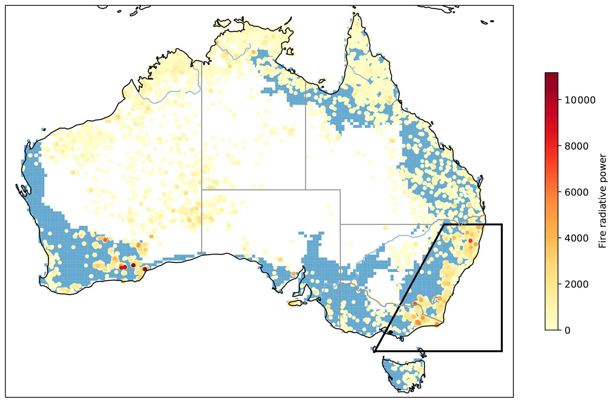
Figure 1Moderate Resolution Imaging Spectroradiometer (MODIS) active fire data (Collection 6, near-real-time and standard products) showing the severity of bushfires from 1 October 2019 to 10 January 2020 with the most severe fires being depicted in red. The image also shows the forested areas in blue. The polygon shows the area analysed in this article.
Wildfires in general are one of the most complex weather-related extreme events (Sanderson and Fisher, 2020) with their occurrence depending on many factors including the weather conditions conducive to fire at the time of the event and also on the availability of fuel, which in turn depends on rainfall, temperature and humidity in the weeks, months and sometimes even years preceding the actual fire event. In addition, ignition sources and type of vegetation play an important role. The types of vegetation depend on the long-term climatology but do not vary on the annual and shorter timescales we consider, and the dry thunderstorms providing a large fraction of the ignition sources are too small to analyse with climate models. In this analysis we therefore only consider the influence of weather and climate on the fire risk, excluding ignition sources, types of vegetation and weather caused by the fires such as pyrocumulonimbus development. There is no unified definition of what fire weather consists of, as the relative importance of different factors depends on the climatology of the region. For instance, fires in grasslands in semi-arid regions behave very differently than those in temperate forests. There are a few key meteorological variables that are important: temperature, precipitation, humidity and wind (speed as well as direction). Fire danger indices are derived from these variables either using physical models or empirical relationships between these variables and fire occurrence, including observed factors such as the rate of spread of fires and measurements of fuel moisture content with different sets of weather conditions.
Southeastern Australia experiences a temperate climate, and on the eastern seaboard hot summers are interspersed with intense rainfall events, often linked with “east-coast lows” (Pepler et al., 2014). Bushfire activity historically commences in the Austral spring (September–November) in the north and summer (December–February) in the south (Clarke et al., 2011). In Australia the Forest Fire Danger Index (FFDI, McArthur, 1966, 1967; Noble et al., 1980) is commonly used for indicating dangerous weather conditions for bushfires, including for issuing operational forecasts during the 2019/20 summer. The index is based on temperature, humidity and wind speed on a given day as well as a drought factor, which is based on antecedent temperature and rainfall.
Bushfire weather risk, as characterized by the FFDI, has increased across much of Australia in recent decades (Clarke et al., 2013; Dowdy, 2018; Harris and Lucas, 2019). Similar, increasing trends in fire weather conditions over southern Australia have been identified in other studies, both for the FFDI (e.g. Dowdy, 2018) and for indices representing pyroconvective processes (Dowdy and Pepler, 2018). These observed trends over southeastern Australia are broadly consistent with the projected impacts of climate change (e.g. Clarke et al., 2011; Dowdy et al., 2019). For individual fire events, studies have shown that it can be difficult to separate the influence of anthropogenic climate change from that of natural variability (e.g. Hope et al., 2019; Lewis et al., 2020).
An alternative index is the physically based Canadian Fire Weather Index (FWI) that also includes the influence of wind on the fuel availability (Dowdy, 2018). The latter is achieved by modelling fuel moisture on three different depths including the influence of humidity and wind speed on the upper fuel layer (Krikken et al., 2019). While the FWI was originally developed specifically for the Canadian forests, the physical basis of the models allows it to be used for many different climatic regions of the world (e.g. Camia and Amatulli, 2009; Dimitrakopoulos et al., 2011) and has been shown to provide a good indication of the occurrence of previous extreme fire events in the southeastern Australian climate (Dowdy et al., 2009). A study on the emergence of the fire weather anthropogenic signal from noise indicated that this is expected around 2040 for southern Australia (Abatzoglou et al., 2019) using the FWI. In this study we also consider the monthly severity rating (MSR), which is derived from the FWI and better reflects how difficult a fire is to suppress (Shabbar et al., 2011). A more detailed analysis of the FWI in the context of bushfires in southeastern Australia is given in Sect. 2.1.
As the fire risk indices depend on heat and drought and these were also extreme in 2019/20, we also consider these factors separately. Previous attribution studies on Australian extreme heat at regional scales have generally indicated an influence from anthropogenic climate change. The “Angry Summer” of 2012/13 – which until 2018/19 was the hottest summer on record – was found to be at least 5 times more likely to occur due to human influence (Lewis and Karoly, 2013). The frequency and intensity of heatwaves during this summer were also found to increase (Perkins et al., 2014). Other attribution assessments that found an attributable influence on extreme Australian heat include the May 2014 heatwave (Perkins and Gibson, 2015), the record October heat in 2015 (Hope et al., 2016) and extreme Brisbane heat during November 2014 (King et al., 2015a). However, at small spatial scales, human influence on extreme heat is sometimes less clear, as in Melbourne in January 2014 (Black et al., 2015). It is worth noting that Lewis et al. (2020) found that the temperature component of the extreme 2018 Queensland fire weather had an anthropogenic influence, while no clear influence was detected on the February 2017 extreme fire weather over eastern Australia (Hope et al., 2019). We are not aware of any extreme event attribution studies on Australian drought.
Thus, while it is clear that climate change does play an important role in heat and fire weather risk overall, assessing the magnitude of this risk and the interplay with local factors has been difficult. Nevertheless it is crucial to prioritize adaptation and resilience measures to reduce the potential impacts of rising risks.
We perform the analysis of possible connections between the fire weather risk and anthropogenic climate change in three steps. First, we assess the trends in extreme temperature and conduct an attribution study using the annual maximum of the 7 d moving average of daily maximum temperatures corresponding to the timescale chosen for the FWI (Sect. 3). Second, we undertake the same analysis but for meteorological drought (i.e. defined purely as a lack of rainfall) in two time windows, the annual precipitation as well as the driest month within the fire season, which is September–February in our study area (Sect. 4). The latter again roughly corresponds to the timescale on which precipitation deficits factor into the FWI, namely 52 d. Third, and most importantly, we conduct an attribution study on the FWI and MSR as indices of the probability of bushfires due to the weather (Sect. 5). These three attribution studies follow the same protocol used in previous assessments: heat waves in Kew et al. (2019), low precipitation in Otto et al. (2018b), and the Fire Weather Index in Krikken et al. (2019). The full and generalized event attribution protocol has recently been documented in Philip et al. (2020). In order to condense the lengthy analysis, we provide short overviews of the heat and drought analysis in the main paper, with extensive results in the Supplement, and focus primarily on the FWI and MSR analysis. We also provide a short analysis and discussion of other large-scale drivers that were of potential importance during 2019/20, such as El Niño–Southern Oscillation (ENSO), the Indian Ocean Dipole (IOD) or the Southern Annular Mode (SAM), in Sect. 6 with a detailed analysis in Sect. S3. Finally, we briefly discuss non-climate factors, such as exposure and vulnerability, that have contributed to the impacts of the extreme fire season of 2019/20.
2.1 General event definition
Since we are investigating several different indicator or driver variables of fire risk, different event definitions are developed for different variables. The details of those definitions are given at the beginning of the respective sections on temperature, precipitation and fire weather indices (Sects. 3–5). General parameters of the event definition are given here.
The fire season (September–February) serves as the general event time window, and the region with the most intense fires in 2019/20 in southeastern Australia serves as the general event spatial domain; specifically this is the land area in the polygon 29∘ S, 155∘ E; 29∘ S, 150∘ E; 40∘ S, 144∘ E; and 40∘ S, 155∘ E (as shown in Fig. 1), which corresponds to the area between the Great Dividing Range and the coast.
The primary way we investigate the connection between anthropogenic climate change and the likelihood and intensity of dangerous bushfire conditions is through the FWI. The FWI provides a reasonable proxy for the burned area in the extended summer months, with the strongest relationship observed from November to February. Figure 2 shows both the Spearman rank correlation and the Pearson correlation of the FWI with log-transformed burned area. The 95 % confidence intervals are also shown. Given the similarity in the correlation coefficients (r) within their confidence intervals, the log-linear relationship appears to explain equal variability (r2) to that of the ranks.
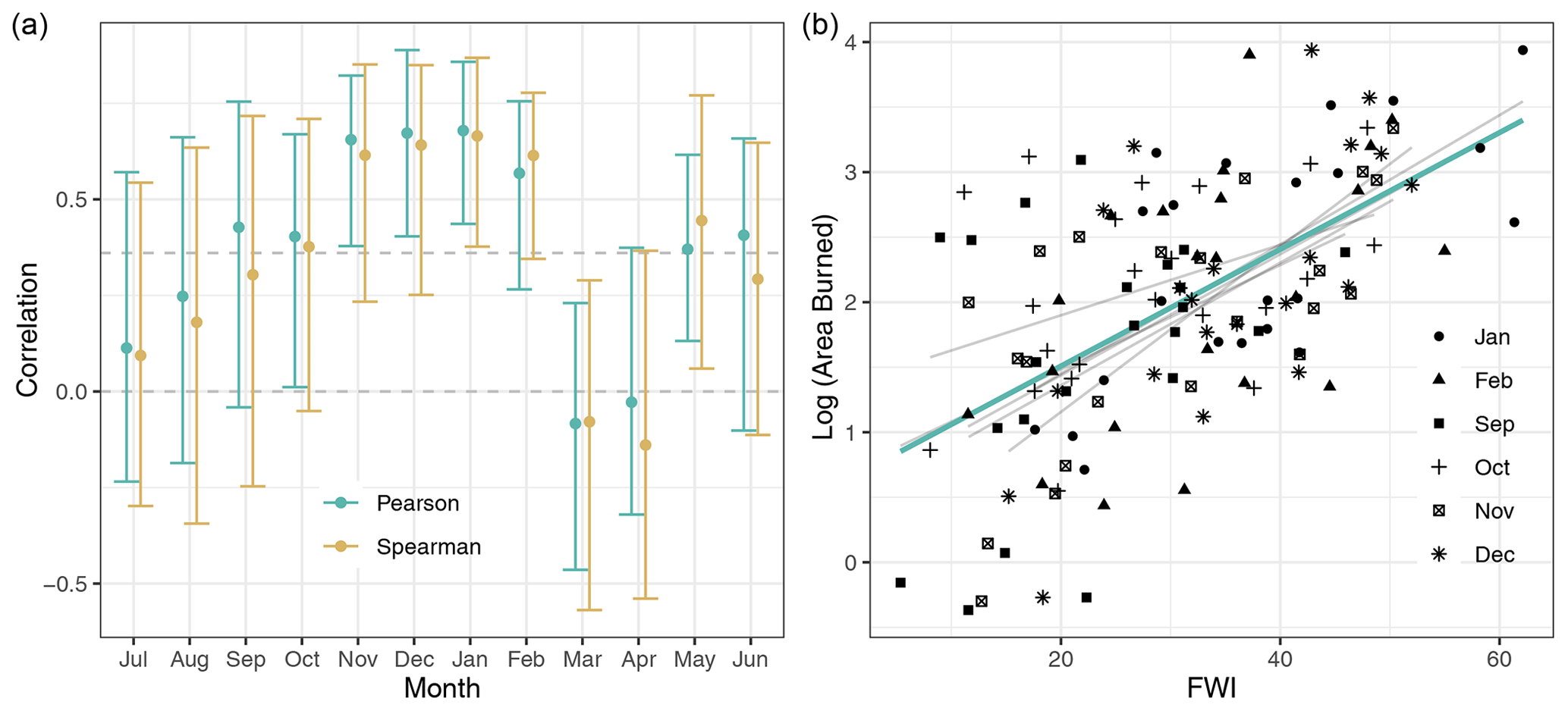
Figure 2(a) Correlation between the logarithm of area burned (10log (km2), MODIS Collection 6) in the event domain and the 7 d maximum Fire Weather Index for each month of the year. The correlations are based on the years 1997 to 2018, and the 95 % two-sided confidence interval is based on bootstrapping those years. The horizontal line denotes the 5 % significance critical value for a one-sided test of the null hypothesis that the correlation is zero against the alternative hypothesis that the correlation is positive. (b) Scatterplot and regression line of the values for each month of the fire season (September–February). The grey lines denote the regression lines for the individual months; the green line is for all months in the fire season.
To capture spatial variations in the start of the fire season at a given location within the event domain, we take for most quantities first the maximum per grid point over the fire season (September–February) and next the spatial average over the general event domain. This way the events do not need to be simultaneous at separate grid points within the region. We therefore investigate the question how anthropogenic climate change influences the chances of an intense bushfire season, rather than focusing on a single episode of intense bushfires.
In most years only very small areas are burned, but the observational record also includes events with extremely large areas. Given this, we checked if the burned-area observations were heavy-tailed (Pasquale, 2013). We found that monthly burned area was not Pareto distributed and instead is reasonably approximated using a log-normal distribution. This supports using the log transformation and extrapolating this relationship to the 2019/20 fire season. Temporal detrending of the observations did not alter these conclusions.
2.2 Observational data
The observational data used in this study are described in Sects. S1 and S2 in the Supplement and 5.3 for heat, drought and the Fire Weather Index, respectively, including justifications for including or excluding certain datasets for certain research questions. For the global mean surface temperature (GMST) we use GISTEMP (Goddard Institute for Space Studies Surface Temperature Analysis) surface temperature (Hansen et al., 2010).
2.3 Model and experiment descriptions
Attributing observed trends to anthropogenic climate change can only be done with physical climate models, as they allow for isolating different drivers. For this purpose we included as large a set of ocean–atmosphere coupled and atmosphere-only (i.e. sea surface temperature (SST) prescribed) climate model ensembles as we could find within the time constraints of this study in order to obtain estimates of both the uncertainty due to natural variability and the model uncertainty. A selection of large ensembles of climate models from the Coupled Model Intercomparison Project Phase 5 (CMIP5) has been used: CanESM2 (Canadian Earth System Model), CESM1-CAM5 (Community Earth System Model–Community Atmosphere Model), CSIRO Mk3.6.0 (Commonwealth Scientific and Industrial Research Organisation), EC-Earth 2.3 (European community earth system model), GFDL CM3 (Geophysical Fluid Dynamics Laboratory Climate Model), GFDL ESM2M (GFDL Earth System Model 2) and MPI-ESM (Max Planck Institute for Meteorology Earth System Model). In addition, the HadGem3-A N216 (Hadley Centre Global Environment Model) attribution model developed in the EUropean CLimate and weather Events: Interpretation and Attribution (EUCLEIA) project, the weather@home (HadAM3P, Hadley Centre atmosphere model) distributed attribution project model, and the ASF-20C (Atmospheric Seasonal Forecasts of the 20th Century) seasonal hindcast ensemble have been used. These last three models are uncoupled and forced with observed historical SSTs and estimates of SSTs, as they might have been in a counterfactual world without anthropogenic climate change. Finally, we used the coupled IPSL-CM6A-LR (Institut Pierre‐Simon Laplace Climate Model) low-resolution CMIP6 ensemble. The GFDL-CM3 and MPI-ESM models that did not have daily data were not used for the extreme-heat analysis. A list of these climate models and their properties is given in Table 1. For the FWI analysis, which requires daily data of relative humidity (RH), temperature, precipitation and wind speed, the list of models used is shortened to CanESM2, CESM1-CAM5, EC-Earth, IPSL-CM6A-LR and weather@home.
Weisheimer et al. (2017)Kirchmeier-Young et al. (2017)Kay et al. (2015)Jeffrey et al. (2013)Hazeleger et al. (2010)Sun et al. (2018)Rodgers et al. (2015)Ciavarella et al. (2018)Boucher et al. (2020)Maher et al. (2019)Guillod et al. (2017)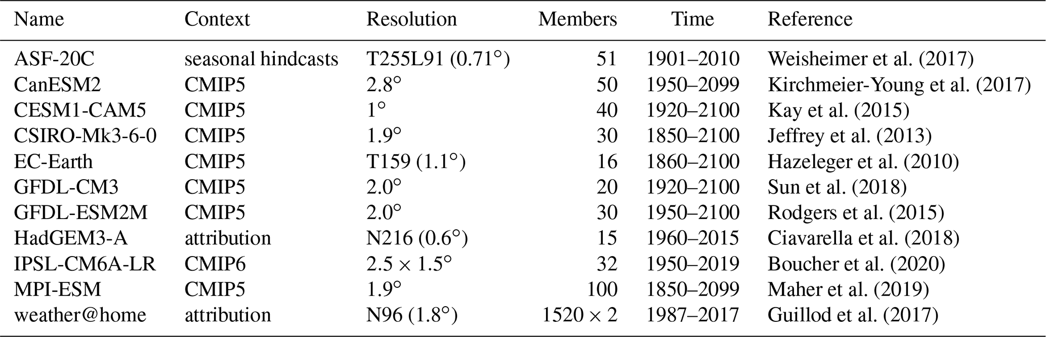
2.4 Statistical methods
The methods employed in this analysis have been used previously for high and low temperatures (van Oldenborgh et al., 2015; King et al., 2015b; van Oldenborgh et al., 2018; Philip et al., 2018a; Kew et al., 2019), extreme precipitation (Schaller et al., 2014; Siswanto et al., 2015; Vautard et al., 2015; Eden et al., 2016; van Oldenborgh et al., 2016; van der Wiel et al., 2017; van Oldenborgh et al., 2017; Eden et al., 2018; Otto et al., 2018a; Philip et al., 2018b), drought (King et al., 2016; Martins et al., 2018; Otto et al., 2018b; Philip et al., 2018c; Uhe et al., 2018) and forest fire weather (Krikken et al., 2019). A paper describing the methods in detail was recently published as Philip et al. (2020).
Changes in the frequency of extreme events are calculated by fitting the data to a statistical distribution. In this study the highest temperature extremes and fire-risk-related variables (FWI and MSR) of the fire season are assumed to follow a generalized extreme value (GEV) distribution, which is the distribution that block maxima converge to Coles (2001). While our event definition is not exactly block maxima, the GEV fits the data well (see below for more details). The low values of annual mean precipitation and lowest monthly precipitation of the fire season are fitted using a generalized Pareto distribution (GPD), which describes the exceedance below a low threshold and also allows for the specification of a threshold that ensures the PDF (probability density function) is zero for negative precipitation.
The GEV distribution is
where x the variable of interest, e.g. temperature or precipitation. Here, μ is the location parameter; σ>0 is the scale parameter; and ξ is the shape parameter. The shape parameter determines the tail behaviour: a negative shape parameter gives an upper bound to the distribution, for ξ≥1 the tall is so fat that the mean is infinite. The scale parameter corresponds to the variability in the tail.
The GPD gives a two-parameter description of the tail of the distribution above a threshold, where the low tail of precipitation is first converted to a high tail by multiplying the variable by −1. The GPD is then described by
with x being the temperature or precipitation, u being the threshold, σ being the scale parameter, and ξ being the shape parameter determining the tail behaviour. For the low extremes of precipitation, the fit is constrained to have zero probability below zero precipitation (ξ<0, σ<uξ). Calculations were conducted on the lowest 20 % and 30 % of the data, which provide a first-order estimate of the influence of using more or less extreme events. We cannot use less data, as the maximizations of the likelihood function do not converge anymore, and using more than 30 % would not qualify as the “lower tail”.
Drought (or low precipitation) is particularly difficult to model using the existing extreme value framework (Cooley et al., 2019). While minima can be modelled by multiplying by −1 (Coles, 2001), the applicability of the underlying extreme value theory assumptions still needs to be validated. In the case of low precipitation, year-on-year autocorrelations are a concern. In southeastern Australia, these serial autocorrelations are approximately r≈0.2, so although they are non-zero, they do not dominate the drought characteristics. Despite these theoretical limitations, in practice the diagnostic plots show that the generalized Pareto models are able to describe the data reasonably well. In particular, they respect that precipitation is non-negative. In general this is a difficult problem, and the statistical extremes community is developing solutions necessary for modelling drought events (Naveau et al., 2016).
To calculate a trend in transient data, some parameters in these statistical models are made a function of the 4-year smoothed global mean surface temperature (GMST) anomaly T′. This smoothing is the shortest that on the one hand reduces the ENSO component of GMST, which is not externally forced and therefore not relevant for the trend, but on the other hand it retains as much of the forced variability as possible (Haustein et al., 2019). A longer smoothing timescale would create problems with extrapolation in the highly relevant last few years of the instrumental record. The covariate-dependent function can be inverted and the distribution evaluated for a given year, e.g. a year in the past (with ) or the current year (). This provides estimates and confidence intervals of the probabilities for an event at least as extreme as the observed one in these 2 years, p0 and p1, or expressed as return periods and . The change in probability between 2 such years is called the probability ratio (PR): . We also estimate the changes in intensity (including uncertainties): ΔT for temperature, ΔP for drought and ΔFWI.
For extreme temperature we assume that the distribution shifts with GMST as or and σ=σ0 with α denoting the trend, which is fitted together with μ0 and σ0. The shape parameter ξ is assumed constant. For drought and FWI-related variables we instead make the assumption that the distribution scales with GMST, the scaling approximation (Tebaldi and Arblaster, 2014). In a GEV fit this gives
and in a GPD fit, it is
with fit parameters σ0, α and ξ. The threshold u0 is determined with an iterative procedure, and the shape parameter ξ is again assumed constant. The exponential dependence on the covariate is in this case just a convenient way to ensure a distribution that is zero for negative precipitation and has no theoretical justification. For the small trends in this analysis it is similar to a linear dependence.
The validity of the other assumption, that the scale parameter or dispersion parameter are constant, is tested by computation of the significance of deviation of a constant of running (relative) variability plots of the observations and model data (Philip et al., 2020). The analysis of model data is more sensitive to variations of these parameters over time due to the large number of ensemble members but of course assumes the effect of external forcing on the variability is modelled correctly.
For all fits we also estimate 95 % uncertainty ranges using a non-parametric bootstrap procedure, in which 1000 derived time series, generated from the original one by selecting random data points with replacement, are analysed in exactly the same way. The 2.5th and 97.5th percentile of the 1000 output parameters (defined as with i being the rank) are taken as the 95 % uncertainty range. For some models with prescribed SSTs or initial conditions (in the case of the seasonal forecast ensemble) the ensemble members are found to not be statistically independent, defined here by a correlation coefficient with e≈2.7182. In those cases the same procedure is followed except that all dependent time series are entered together in the bootstrapped sample, analogous to the method recommended in Coles (2001) to account for temporal dependencies.
When using a GEV to model tail behaviour, note that taking the spatial average of the annual maxima does not have the same statistical justification as taking the annual maximum of the spatial average (Coles, 2001). Given this, the impact of the order of operations in the event definition was examined. For the temperature extremes, we compared the time series where we first take the annual maximum and next the spatial average to the definition with the order reversed, which can be approximated with a GEV. The Pearson correlation was r=0.95, which is likely due to strong spatial dependence and the concentration of heatwaves at the peak of the seasonal cycle. Therefore, in practice, an approximation with a GEV is not entirely unsuitable for temperature, but caution should be exercised. For the FWI and MSR, the order of operations does make a clear difference. Indeed, we find that the whole distribution is not described well by a GEV for one climate model used (CanESM2). For that model we take block maxima over five ensemble member blocks, effectively looking only at the most extreme events. For this part of the distribution the GEV fit agrees with the data points in the return time plot, as expected from taking block maxima.
We evaluate all climate models on the fitting parameters by determining whether the model-derived parameters fall within the uncertainty range of observation-derived parameters. We allow for a mean bias correction; i.e. we only check the scale and shape parameters σ and ξ. Model biases are accounted for by evaluating the model at the same return time as the value found in the observational analysis. This was found to give better results than applying an additive or multiplicative bias correction to the position parameter μ, as it also corrects to first order for biases in the other parameters, especially when the distribution has an upper or lower bound (ξ<0), which is the case in all the cases here.
Finally, estimates of the PR and change in observations and all climate models that pass the evaluation test are combined to give a synthesized attribution statement. First, the observations and reanalyses were combined by averaging the best estimate and lower and upper bounds, as the natural variability is strongly correlated, as they are largely based on the same observations (except for the long reanalyses). The difference is added as representation uncertainty (white extensions on light-blue bars in Figs. S6, S12, S13 and 6).
Second, the model results were combined by computing a weighted average (using inverse model total variances), as the natural variability in the models, in contrast to the observations, is uncorrelated:
with being the estimated uncertainty in model i and Xi being either the temperature or the logarithm of precipitation, FWI or MSR. The sums are over the Nmod models. Using this we can compare the spread expected from the natural variability with the observed spread of the model results using χ2 statistics:
If , with dof being the number of degrees of freedom, here N−1, the spread of the results is compatible with the uncertainty estimated from the fits due to variability within the climate model, and the results can be taken to be independent estimates of X and the weighted average used. However, if the model spread is larger than expected from variability due to sampling of weather noise alone, so a model spread term was added to each model in addition to the weighted average (white extensions on the light-red bars, Figs. S5 and S6) to account for systematic model errors. This term is defined by requiring that . The total uncertainty of the models is shown as a bright-red bar in these figures. This total uncertainty consists of a weighted mean using the uncorrelated natural variability plus an independent model spread term added to the uncertainty if , which we do not divide by ; i.e. we do not assume that by adding more models to the ensemble the model uncertainty decreases. This procedure is similar to the one employed by Ribes et al. (2020).
Finally, observations and models are synthesized into a single mean and uncertainty range. This can only be done when they appear to be compatible. We show two combinations. The first one is computed by neglecting model uncertainties beyond the model spread. The optimal combination is then the weighted average of models and observations, shown as a magenta bar. However, the total model uncertainty is unknown and can be larger than the model spread. We therefore also show the more conservative estimate of an unweighted average of observations and models with a white box in the synthesis plots.
The key takeaways from the attribution analysis of trends in extreme heat are summarized here, while the details are given in Sect. S1.
Taking advantage of the longer observational record for temperature than for other variables, we analyse the highest 7 d mean maximum temperatures of the year (TX7x), averaged over the event domain (Fig. 1), from 1910 (the beginning of standardized temperature observations) to 2019.
Observations show that a heatwave as rare as observed in 2019/20 would have been 1 to 2 ∘C cooler at the beginning of the 20th century (Fig. S6). Similarly, a heatwave of this intensity would have been less likely by a factor of about 10 in the climate around 1900 (Fig. S6). While climate models consistently simulate increasing temperature trends over this time period, they all have some limitations for simulating heat extremes: the variability of 7 d mean maximum temperature is generally too high, and the long-term trend is only 1 ∘C (Figs. S5 and S6). We can therefore only conclude that anthropogenic climate change has made a hot week like the one in December 2019 more likely by at least a factor of 2 but cannot give a best estimate or upper bound due to the model deficiencies limiting our confidence in the exact magnitude of the anthropogenic influence.
The reasons for the apparent model deficiencies in simulating trends and variability in extreme temperatures are not fully understood. In Sect. S3 we show that the temperature variability explained by the Indian Ocean Dipole (IOD) and Southern Annual Mode (SAM) is too small to explain these mismatches as problems in the model representation of these modes of variability. The literature suggests that shortcomings in the coupling to land and vegetation (e.g. Fischer et al., 2007; Kala et al., 2016) and in parametrization of irrigation (e.g. Thiery et al., 2017; Mathur and AchutaRao, 2019) in the exchange of heat and moisture with the atmosphere and also in the representation of the boundary layers (e.g. Miralles et al., 2014) are more likely to be the cause of the problems. Given the larger trend in observations than in the models we suspect that climate models underestimate the trend in extreme temperatures due to climate change, although in principle the difference could also be due to a non-climatic driver that affects the trend in observations. The combination of a weaker trend and higher variability in models compared to observations yields an increase in the likelihood of such an event that is much higher in observations than in models.
The key takeaways from the attribution analysis of trends in low precipitation are summarized here, while the details are given in Sect. S2. The conclusions below are shown in Fig. S12 for annual mean drought, and those in Fig. S13 are for the driest month of the year.
Observations show non-significant trends towards more dry extremes like the record 2019 annual mean and a non-significant trend towards fewer dry months like December 2019 in the fire season (Figs. S12 and S13). All 10 climate models we considered simulate the statistical properties of the observations well (Figs. S10 and S11). Collectively they show trends neither in dry extremes of annual mean precipitation nor in the driest month of the fire season (September–February). We conclude that there is no evidence for an attributable trend in either kind of meteorological drought extremes like the ones observed in 2019.
5.1 The fire weather of 2019/20
As discussed in the introduction, the fire risk as described by fire weather indices was extreme in the study domain in the 2019/20 fire season. The domain was chosen to encompass these fires, and therefore the 2019/20 event cannot be included in the statistical analysis.
5.2 Temporal event definition
We choose two event definitions in order to represent two important aspects of the event, namely the intensity and the duration. For intensity, we first select the maximum FWI of a 7 d moving average over the fire season (September–February) for every grid point over the study region, after which we compute the spatial average, hereafter FWI7x-SM (seasonal maximum). The 7 d timescale was chosen based on a good correlation with the area burned (see Fig. 2) and good correspondence with area burned in other forest fire attributions studies (Krikken et al., 2019).
For duration, we consider the monthly severity rating (MSR). The MSR is the monthly averaged value of the daily severity rating (DSR), which in turn is a transformation of the FWI (DSR=0.0272FWI1.71). The DSR reflects better how difficult a fire is to suppress, while the MSR is a common metric for assessing fire weather on monthly timescales (Van Wagner, 1970). For this study, we select the maximum value of the MSR during the fire season over the study area (MSR-SM). In contrast to the FWI7x-SM, we first apply a spatial average of the study area and then select the maximum value per fire season. This event definition focuses more on changes in extreme fire weather for longer timescales and larger integrated areas than FWI7x-SM. Note that neither of the two event definitions includes ignition sources or small-scale meteorological factors such as pyrocumulonimbus development that could enhance the fires.
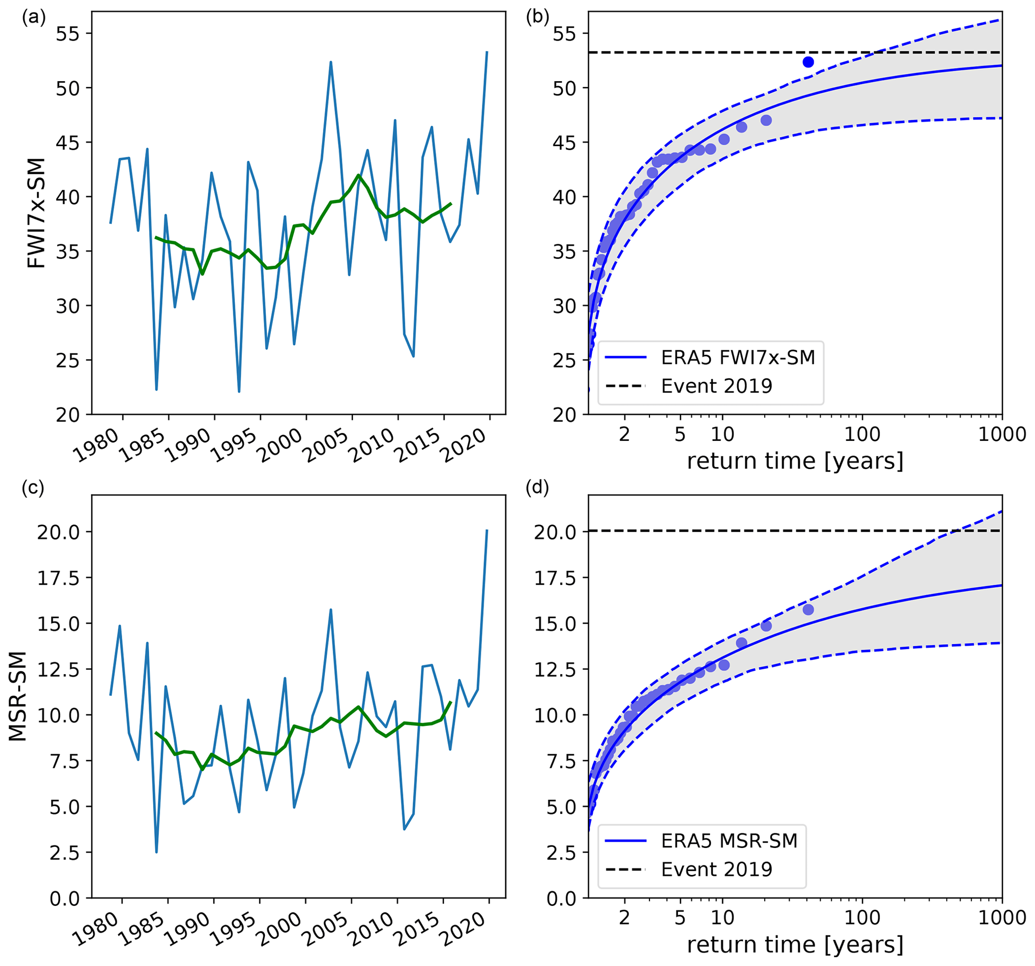
Figure 3(a, c) Time series with the 10-year running mean of the area average of the highest 7 d mean Fire Weather Index in September–February (a) and maximum of the monthly severity rating in September–February (c). (b, d) Stationary GEV fit to these data; the dots represent the ordered years, and the grey bands represent the 95 % uncertainty ranges.
5.3 Observational analysis: return time and trend
For the observational analysis we use the fifth-generation European Centre for Medium-Range Weather Forecasts (ECMWF) Atmospheric Reanalysis (ERA5) dataset for 1979–January 2020 (Hersbach et al., 2019). This reanalysis dataset is heavily constrained by observations and thus provides one of the best estimates of the actual state of the atmosphere for all the variables needed to compute the FWI over the study area. Other reanalyses did not yet include the full 2019/20 event at the time of the analysis.
Figure 3 shows the time series of the highest 7 d mean FWI averaged over the study area. Both for the FWI7x-SM and MSR-SM the event is the highest over the 1979–2020 time period. Note that for the MSR-SM, the value is considerably more extreme than for the FWI7x-SM. The GEV fits (Fig. 3, right) illustrate this further, with return times in excess of 1000 years.
A fit allowing for scaling with the smoothed GMST gives a significant trend in the FWI7x-SM (Fig. 4). This fit gives a return time for the 2019/20 fire season of about 31 years (4 to 500 year) in the current climate and more than 800 years extrapolated to the climate of 1900. This corresponds to an infinite PR, with a lower bound of 4. The return time for the MSR-SM is undefined and is thus estimated to be 100 years. For the climate model analysis we thus use return times of 31 years for the FWI7x-SM and 100 years for the MSR-SM to determine the event thresholds in individual climate models.
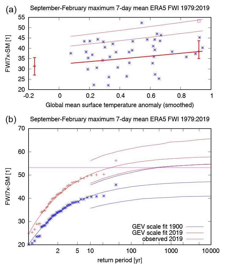
Figure 4Fit of a GEV that scales with the smoothed GMST (Eqs. 1 and 3) of the highest 7 d mean FWI computed from the ERA5 reanalysis, averaged over the index region. (a) Observations (blue symbols), location parameter μ (thick line and uncertainties in 1900 (extrapolated) and 2019/20), and the 6 and 40 year return values (thin lines). The purple square denotes the 2019/20 value, which is not included in the fit. (b) Return time plot with fits for the climates of 1900 (blue lines with 95 % confidence interval) and 2019 (red lines); the purple line denotes the 2019/20 event. The observations are plotted twice, shifted down to the climate of 1900 (blue stars) and up to the climate of 2019 (red pluses) using the fitted dependence on smoothed global mean temperature so that they can be compared with the fits for those years.
5.4 Model evaluation
We use four climate models with large ensembles, leaving out CESM1-CAM5 because of its failure to represent heat extremes (see Sect. 3). This is fewer than for the drought and heat analysis because the FWI requires four daily input variables, which are not available for all models. In contrast to the heat extremes and drought analyses, the fits to the model output use as covariate the model GMST. We also define our reference climates using GMST rather than years. The years at which the climate is evaluated are taken from the 1.1 ∘C temperature increase for the present-day climate and the 2 ∘C increase for the future reference climate and not 2019 and 2060. As the fits are invariant under a scaling of the covariate, this does not make much difference.
First the models are evaluated on how well they represent the extremes of the FWI7x-SM and MSR-SM. This is quantified by the dispersion parameter and shape parameter ξ of the GEV fit for the present-day climate. We do not check the position parameter μ, assuming a multiplicative bias correction can be applied.
Figure 5 gives an overview of these parameters. Preferably, we would like the parameters to lie within the observational uncertainty of ERA5. For the dispersion parameter CanESM2 and weather@home fall within the observational uncertainty of the FWI. The other two models (EC-Earth and IPSL CM6) show too much variability relative to the mean. The same holds for the shape parameter. This implies that it is difficult to draw strong conclusions from the model data, given that they do not accurately represent the extremes of the FWI7x-SM. In particular, the models with too much variability will underestimate the probability ratios. We continue with all four models but keep these problems in mind.
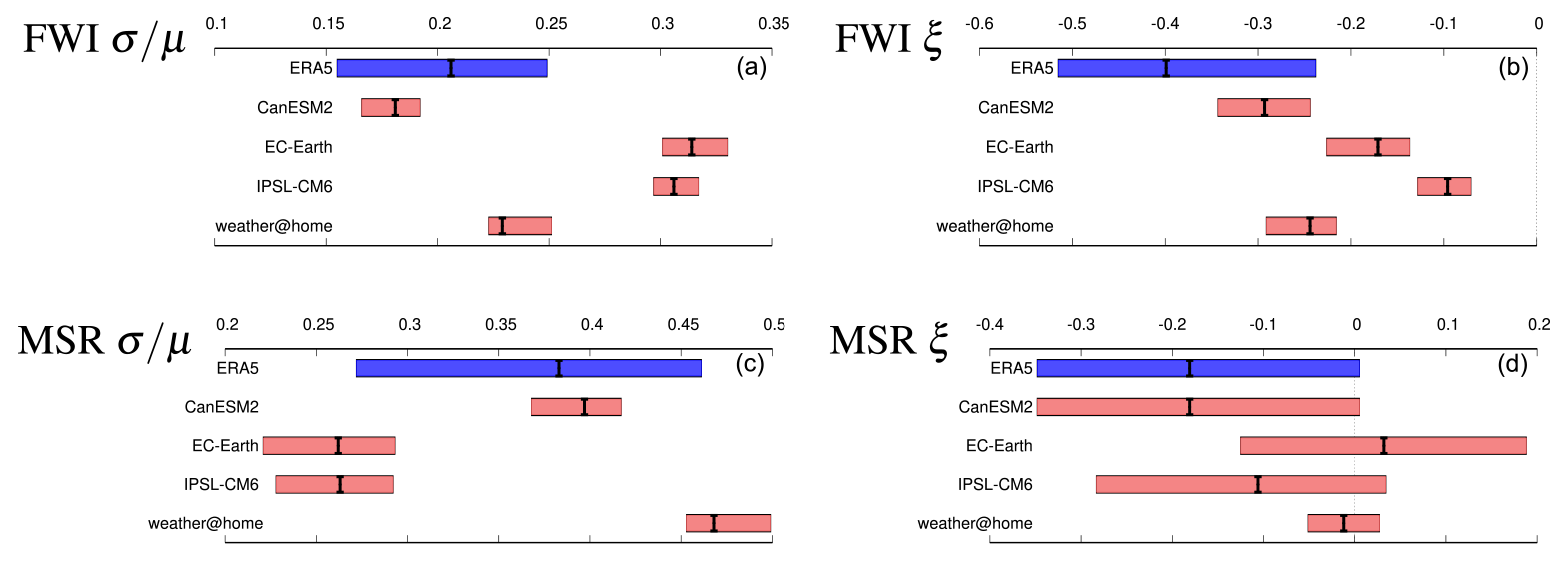
Figure 5Model verification for the FWI (a, b) and MSR (b, c). The left figures show the dispersion parameter , and the right figures show the shape parameter ξ. The bars denote the 95 % uncertainty ranges.
The MSR is simulated better: all model dispersion and shape parameters lie within the large observational uncertainties, although they largely disagree with one another on the dispersion parameter.
5.5 Multi-model attribution and synthesis
The model results are summarized by their PR, i.e. how more or less likely such an event will be for present or future climate, relative to the early 20th century.
Figures 6 and 7 show the change in probability for both the FWI7x-SM and the MSR-SM from 1920 to 2019 (denoting the 2019/20 fire season). For the FWI7x-SM, all models agree on an increased probability for such an event in the present climate relative to the early 20th century, although the trend is not significant at p<0.05 (two-sided) for one of the models, CanESM2. As the spread of the models is compatible with natural variability (), we take a weighted average across the models to synthesize them (Fig. 6). This shows that such an event has become about 80 % more likely in the models, with a lower bound of 30 %. Note that all models severely underestimate the increased risk compared to ERA5, which has a lower bound of the PR of a factor of 4 relative to 1920 (extrapolated), above the upper end of the model average. Note that the ERA5 value is probably biased high, as the positive contribution of trend towards a drier climate over 1979–2019 is not present over 1900–2019; see Sects. S2 and 5.6.
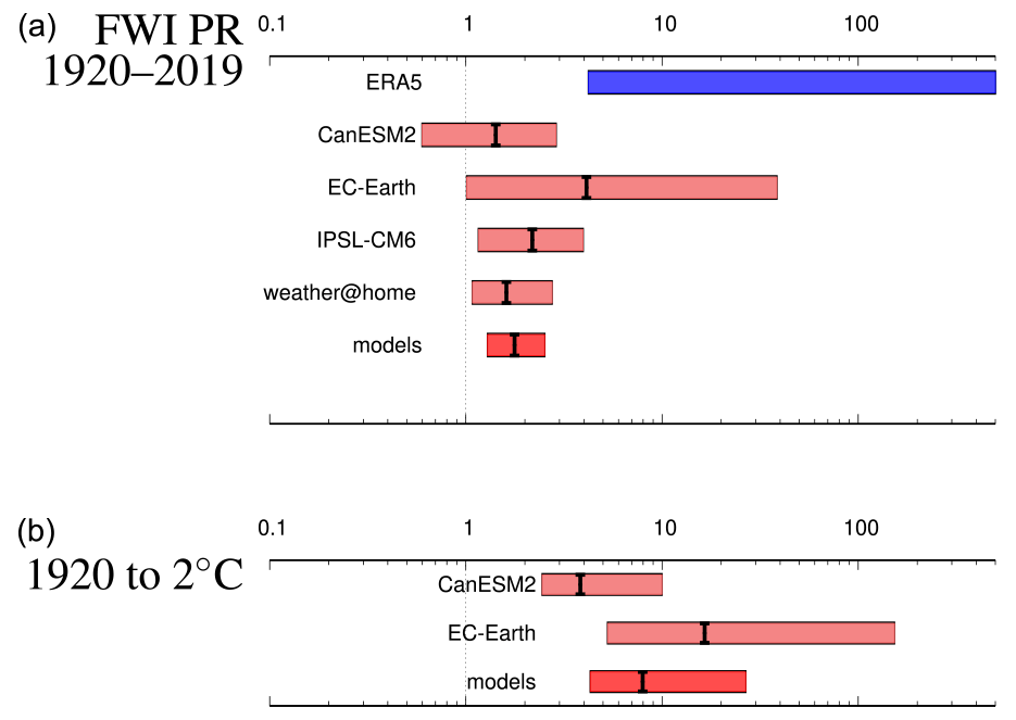
Figure 6(a) The PR for an FWI as high as observed in 2019/20 or higher: (a) from 1920/21 to 2019/20 and (b) from 1900 to a climate globally 2 ∘C warmer than 1920. The last row is the weighted average of all models, the spread of which is consistent with only natural variability. (b) Same for a 2 ∘C climate (GMST change from the late 19th century).
For a future climate of 2 ∘C warming above pre-industrial levels we find that such events become about 8 times more likely in the models, with a lower bound of about 4 times more likely. Note that the estimate of future climate is only based on two climate models, CanESM2 and EC-Earth, due to the absence of future data for the others.
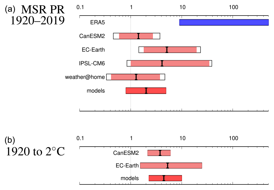
For the MSR-SM the models on average show about a doubling of probability for the present climate relative to the early 20th century (Fig. 7). However, this trend is not significant, as the lower bound is 0.8; i.e. a decreased probability is also possible within the two-sided 95 % uncertainty range. In the fit to the ERA5 data we include 2019, as otherwise the probability of the event occurring in the current climate would be zero, contrary to the fact that it did occur. This fit shows much higher probability ratios, with a lower bound of a factor of 9. As there is no overlap with the model results we cannot combine the model and observational results but only give a conservative lower bound as an observation–model synthesis result. For a future climate relative to the climate of the early 20th century the models show an increase in probability of about 4 times, with a lower bound of 2.
5.6 Interpretation
The underestimation of the observed trend in fire weather indices in all models and the tendency for too much variability in some models is reminiscent of the extreme-temperature results in Sects. 3 and S1.
In order to better understand which input variables cause the long-term increase in the FWI7x-SM and thus the contribution to the 2019/20 FWI7x-SM value, we study the input variables to the FWI7x-SM separately for each model as well as observations. For precipitation we use the cumulative precipitation (90 d) prior to each FWI7x-SM value. We calculate the change from the early 20th century to the present day in each input variable to estimate its long-term change, which we then subtract from that variable's observed value in 2019/20. We then recalculate the FWI7x-SM but use each detrended individual input variables in turn. Each of these newly calculated FWI7x-SM values thus illustrates the influence of the long-term trend in a particular input variable onto the observed 2019/20 FWI7x-SM value. This procedure is applied to models and ERA5. In the models, the ensemble mean change is used to estimate an individual variable's long-term trend, whereas in ERA5 a regression of each variable onto GMST is used to estimate its value in the early 20th century. The results of this analysis for the 2019/20 FWI7x-SM value are shown in Fig. 9.
The sum of the contributions from individual input variables to the 2019/20 FWI7x-SM anomaly match the effect of changing all variables at the same time, so they can be considered linearly additive (Fig. 9). The underestimation of the extreme-temperature trends in the climate models carries over into this analysis such that the temperature contribution to the observed 2019/20 value is underestimated. Despite this underestimation, temperature emerges as the most important variable in EC-Earth and weather@home, as it explains roughly half of the increase in the FWI. For IPSL, the simulated temperature increase explains about a third of the FWI7x-SM increase, together with wind and RH. CanESM2 behaves differently, where it is mainly the decrease of RH that explains the higher FWI7x-SM. Most but not all models analysed here therefore derive the increase in the FWI7x-SM largely from the increase in temperature extremes.
In ERA5 the increase in temperature also appears to be the most important explanatory variable, followed by a decrease in RH and precipitation. As we did not find a significant trend in precipitation over longer time periods, we hypothesize this trend to be due to natural variability over the short 1979–2018 period in ERA5. We explicitly verified that the dependence of the FWI7x-SM on temperature is almost linear in a range of ±5 K around the reanalysis value (not shown). Further, volumetric soil water (Fig. 8) at multiple soil layers from ERA5 suggests that, despite the soil already being very dry in 2018 and into 2019, the 2019/20 austral spring–summer drought caused a further drying of the soil in the study area. This suggests that the drought of late 2019 and high temperatures did indeed cause an additional increase in fire risk over preceding years.
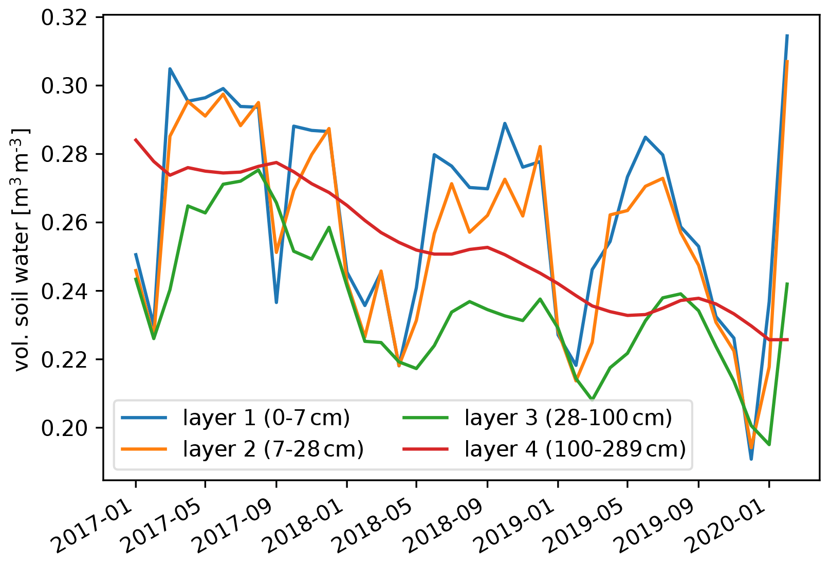
Figure 8ERA5 volumetric soil water from multiple levels. The data represent the spatial average over the study area. Please note that the date format in this figure is year month (yyyy-mm).
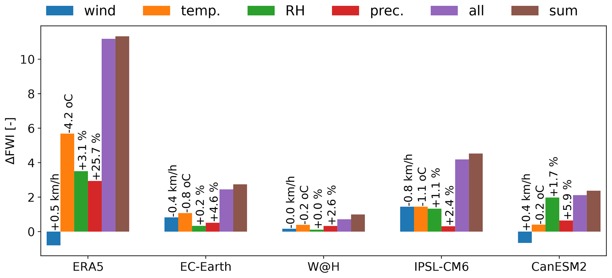
Figure 9Sensitivity analysis of the FWI7x-SM to changes in individual contributions from relative humidity (RH, wind, temperature and precipitation). The relative increases or decreases for the individual variables of the climate models are based on the average change in input variables between the climate of the present day and the early 20th century (values above bars). For ERA5 the changes are based on a linear regression of the respective variable onto GMST for the years 1979 to 2018 and then extrapolated to the early 20th century. These changes are subtracted from the 2019 ERA5 data, after which the FWI is recomputed, where ΔFWI is the original FWI minus the altered FWI. In the “all” experiment all input variables are changed simultaneously. “Sum” is the sum of all the individual changes in the FWI. W@H: weather@home.
5.7 Conclusions fire risk indices
The FWI7x-SM as computed from the ERA5 reanalysis as an approximation to the real world shows that the 2019/20 values were exceptional. They have a significant trend towards higher fire weather risk since 1979. Compared with the climate of 1900, the probability of an FWI7x-SM as high as in 2019/20 has increased by more than a factor of 4. For the MSR-SM the probability has increased by more than a factor of 9.
The four climate models investigated show that the probability of a Fire Weather Index this high has increased by at least 30 % since 1900 as a result of anthropogenic climate change. As the trend in extreme temperature is a driving factor behind this increase and the climate models underestimate the observed trend in extreme temperature, the attributable increase in fire risk could be much higher. This is also reflected by a larger trend in the FWI7x-SM in the reanalysis compared to models. The MSR-SM increased by a factor of 2 in the models since 1900, although this increase is not significantly different from zero. As with FWI7x-SM, the attributable increase is likely higher due to the model underestimation of temperature trends and overestimation of variability in the TX7x.
Projected into the future, the models project that an FWI7x-SM as high as in 2019/20 would become at least 4 times more likely with a 2 ∘C temperature rise, compared with 1900. Due to the model limitations described above this could also be an underestimate.
The attribution statements presented in this paper are for events defined as meeting or exceeding the threshold set by the 2019/20 fire season and thus assessing the overall effect of human-induced climate change on these kinds of events. In individual years, however, large-scale climate system drivers can have a higher influence on fire risk than the trend. A detailed analysis of the influence of ENSO, the IOD and SAM is presented in Sect. S3.
Besides the influence of anthropogenic climate change, the particular 2019 event was made much more severe by a record positive excursion of the Indian Ocean Dipole and a very strong negative anomaly of the Southern Annular Mode, which likely contributed substantially to the precipitation deficit. We did not find a connection of either mode to heat extremes. More quantitative estimates will require further analysis and dedicated model experiments, as the linearity of the relationship between these indices and the regional climate is not verifiable from observations alone.
At least 19.4×10⁶ ha of land has burned as a result of the Black Summer bushfires of 2019/20 (https://disasterphilanthropy.org/disaster/2019-australian-wildfires/, last access: 6 March 2021). This has resulted in 34 direct deaths and the destruction of 5900 residential and public structures (https://reliefweb.int/report/australia/australia-bushfires-information-bulletin-no-4, last access: 7 March 2021). Nearly 80 % of Australians reported being impacted in some way by the bushfires (https://theconversation.com/nearly-80-of-australians-affected-in-some-way-by-the-, last access: 7 March 2021). In Sydney, Canberra and a number of other cities, air quality levels of towns and communities reached hazardous levels (https://www.nytimes.com/interactive/2020/01/03/climate/australia-fires-air.html, last access: 7 March 2021). Over 65 000 people registered on Australian Red Cross' reunification site to look for friends and family or to let loved ones know that they were alright (https://www.redcross.org.au/news-and-media/news/bushfire-response-20-feb-2020, last access: 7 March 2021). It is estimated that over 1.5 billion animals have died nationally (https://reliefweb.int/sites/reliefweb.int/files/resources/IBAUbf050220.pdf, last access: 7 March 2021). These impacts are not only hazard-related but also related to various vulnerability and exposure factors that each play a role in increasing or decreasing risk and impacts. Vulnerability is defined as “The propensity or predisposition to be adversely affected. Vulnerability encompasses a variety of concepts and elements including sensitivity or susceptibility to harm and lack of capacity to cope and adapt” (Agard et al., 2014). It can also be defined as “the diminished capacity of an individual or group to anticipate, cope with, resist and recover from the impact of a natural or man-made hazard” (https://www.ifrc.org/en/what-we-do/disaster-management/about-disasters/what-is-a-disaster/what-is-vulnerability/, last access: 7 March 2021). Exposure is defined as “The presence of people, livelihoods, species or ecosystems, environmental functions, services, and resources, infrastructure, or economic, social, or cultural assets in places and settings that could be adversely affected” (Agard et al., 2014).
Bushfires have been a part of the Australian landscape for millions of years and are an ever-present risk for people living in rural and peri-urban areas surrounded by vegetation, bush and/or grasslands. In recent decades, significant bushfires occurred in 1974/75, 1983, 2002/03 and 2009, some of them including grass fires, which can have different drivers to forest fires like those in 2019/20. This frequent occurrence of severe bushfires, with records extending back to the 1850s, has resulted in robust preparedness and emergency management systems which serve to reduce risk and aid in swift response. Comprehensive risk assessments are undertaken at the level of the local council, and bushfire preparedness and contingency plans have been in place in most high-risk areas for decades. However, these systems were severely strained in the Black Summer bushfires.
7.1 Excess morbidity and mortality
The time of publication is too soon for a robust estimate of excess morbidity and mortality specific to the 2019/20 Australian bushfires. Such analysis is typically available weeks to years following the end of an event. However, the combined impacts of extreme heat and air pollution can be deadly, as seen in the compounded heatwave and wildfire events in 2010 in Russia or 2015 in Indonesia (Shaposhnikov et al., 2014; https://www.nature.com/articles/news.2010.404, last access: 7 March 2021; Koplitz et al., 2016). Those most at risk are the elderly; people with pre-existing cardiovascular, pulmonary and/or renal conditions; and young children, as exposure to wildfire smoke can have acute respiratory effects. Health officials in New South Wales reported a 34 % spike in emergency room visits for asthma and breathing problems between 30 December 2019 and 5 January 2020 (https://www.washingtonpost.com/climate-environment/2020/01/12/australia-air-poses-threat-people-are-rushing-hospitals-, last access: 7 March 2021). One study of hospital admissions in Sydney, Australia, from 1994 to 2010 found that days with air pollution from extreme bushfires (as measured by PM10) resulted in a 1.24 % admission increase for every 10 µg m−3 (Morgan et al., 2010). On the other hand, it should be noted that Australia is a country with a robust healthcare system, which significantly reduces vulnerability to the short- and long-term consequences of smoke and extreme heat.
There is also a need for increased mental health services in the days, weeks and years following severe bushfires. As of January 2020 the Australian government announced AUD 76 million in mental health funding (https://www.abc.net.au/news/2020-01-12/federal-government-funds-for-mental-health-in-fires-crisis/11860660, last access: 7 March 2021). A study of the 2009 Black Saturday bushfires found that while the majority of affected people demonstrated psychological resilience in the long-term aftermath of the fires, a significant minority of people in highly affected communities reported mental health impacts 3–4 years following the event (Bryant et al., 2014).
7.2 Early warning
There is no nationally standardized system for bushfire warnings in Australia. However, recommendations from the royal commission tasked with reviewing the 2009 Victoria bushfire (Teague et al., 2010) have helped to drive forward efforts to establish a national system. In 2014 the National Review of Warnings and Information was undertaken. It recommended the establishment of the dedicated, multi-hazard National Working Group for Public Information and Warnings. Part of the task of this group would be to ensure greater national consistency of early warning information. One outcome of this recommendation is the Public Information and Warnings Handbook, which has been issued to provide guidance to actors across national, state and territory governments in issuing warning information (https://knowledge.aidr.org.au/media/5972/warnings-handbook.pdf, last access: 7 March 2021).
Bushfire warnings in Australia are issued by state and territory fire authorities and generally follow the “Prepare, Stay and Defend or Leave Early” approach. The Fire Danger Rating system is also widely applied as a way to communicate fire risks. The system, originally developed in 1967, contained five risk levels ranging from “low-moderate”, where fires can generally be controlled, to “extreme”, where evacuation is recommended but home defence may be possible under certain circumstances. Following the 2009 Black Saturday bushfires a sixth “catastrophic” level was added where evacuation is deemed the only survival option (https://www.emergency.wa.gov.au, last access: 7 March 2021). This guidance was adopted by all states, except in Victoria where it is called “Code Red” (http://www.bom.gov.au/weather-services/fire-weather-centre/fire-weather-services/index.shtml, last access: 7 March 2021). In 2017, the system was revised to update the metrics used in forecasting the most appropriate level (https://www.abc.net.au/news/2017-12-13/bushfire-danger-rating-system-trialled-summer/9203446, last access: 7 March 2021). Threat level information is provided via radio, television, social media and signs on all major rural roads. Government websites also provide information which is updated every few minutes and includes maps of fires and associated threat levels. In addition, phone calls are made house-to-house when evacuation is recommended.
While these efforts help to reduce vulnerability and exposure to the wildfires, significant barriers to early action still remain. People in bushfire areas are frequently not aware of their risk, are unprepared to manage risk, wait until the final moments to evacuate or, at times, even return to fire-affected areas to defend property (Whittaker et al., 2020). This is particularly relevant in peri-urban areas which are not as frequently exposed to bushfire risks. A 2020 study of people's reactions to bushfire warnings during the 2017 bushfires in New South Wales found that people largely understood warnings but that they did not respond to the warnings before seeking and obtaining additional confirmation to avoid what they might perceive as unnecessary evacuation and associated costs. Researchers recommend that rather than further refining messages, confirmation mechanisms need to be implemented into early warning approaches. There are further barriers to acting on warnings, such as an incorrect assessment of the defensibility of a building, attachments to pets and personal items, and a “hero culture” around people who did defend their home. These sociological barriers to life-saving measures increase the risk of deadly impacts.
Furthermore, an inquiry into the 2009 Black Saturday bushfires found that the Prepare, Stay and Defend or Leave Early approach assumed that individuals had a fire plan in-place, although many people did not. Therefore people were left in a position to make complex decisions without adequate guidance.
7.3 Controlled burning and relation to weather conditions
For this study, we did not assess vegetation cover and condition (dryness) ahead of the season in comparison with earlier years, but it is clear that fire hazard management strategies such as bush reduction, manual removal of undergrowth and controlled burning can affect fire hazard
Note that the effectiveness of such measures depends not only on the type of vegetation but also the specific conditions of the bushfire. For instance, prior controlled burning may be somewhat effective to suppress fire risk under average weather conditions but is much less so in cases of very high temperatures, low humidity and strong wind, i.e. when the fire risk is no longer dominated by the type, condition and quantity of fuel but by weather conditions. During the 2009 fires in Victoria, recently burned areas (up to 5–10 years) may have reduced the intensity of the fires, but they did not enough so as to increase the chance of effective suppression given the severe weather conditions at the time (Price and Bradstock, 2012).
In addition, it should be noted that controlled burning requires a window during the cooler parts of the year when conditions allow for controlled burning to take place. The Queensland Fire and Emergency Services (QFES) noted that controlled burning is highly dependent on weather conditions and that not all planned 2019 burns had been completed, given that in some areas, it rapidly became too dry to burn safely (https://www.abc.net.au/news/2019-12-20/hazard-reduction-burns-bushfires/11817336, last access: 7 March 2021). Recognizing the highly non-linear relationship between weather conditions through the season (and in fact across several years) and anticipatory risk management strategies, in this attribution study we have not assessed the impact of these early-season weather conditions on the ability to reduce risk and thus on fire risk itself.
7.4 Infrastructure and land use planning
Ageing electricity infrastructure may play a role in increasing the risk of bushfire outbreaks from human-related ignition (Teague et al., 2010). Electric-grid fires are primarily due to elastic extension and fatigue failures and are made increasingly worse by high wind speeds (Mitchell, 2013). A 2017 study found that fires sparked by electricity failures are more prevalent during elevated fire risk and tend to burn larger, making them worse than fires due to other causes (Miller et al., 2017). Interestingly, a 2013 report also notes that while electricity operators have the ability to disconnect electricity grids when there is a high risk posed to the public, only South Australia has legislation in place to protect the operator from prosecution (Energy Networks Association, 2013). All of these factors coupled together increase Australia's vulnerability to bushfire outbreaks.
In contrast, stringent building codes have helped to reduce vulnerability to fire risks. The Bushfire Attack Level (BAL), as well as associated building codes, is the guiding resource for assessing and managing risks of a building exposed to heat, embers or direct fire. The BAL is applied nationwide; however the Fire Danger Index, one of the key metrics used in calculating the site-specific BAL, is under state and local level jurisdiction. The highest BAL level was established following the 2009 Black Saturday bushfires (Country Fire Authority, 2012).
Land use planning at a community level is also crucial in reducing bushfire risk, particularly for rural and peri-urban areas which face the highest bushfire risks. This is recognized and addressed through state and local government planning processes, which include ensuring accessible bushfire evacuation routes and spaces. For example, the 2009 Victorian Bushfires Royal Commission cited a need for planning which “prioritized human life over all other policy objectives”. This led to relevant policy changes through an amendment to the Victoria Planning Provisions. The Bushfire Management Overlay and associated guidelines are among the principle aspects of this amendment. They provide direction for approval of new construction locations as well as siting and layout requirements of approved spaces, although these guidelines do not apply to existing property, which puts a limitation on their overall positive impact (Country Fire Authority, 2012).
7.5 Conclusions on vulnerability and exposure
Bushfires are a natural phenomenon, but their impact is also strongly influenced by human choices. Overall, Australia is one of the most prepared countries in the world to manage bushfires, and thus the impacts from this season's bushfire outbreaks could have been dramatically worse if not for the systems in place. This not only underscores the urgent need to adapt to changing risks in all places, with a special focus on the most vulnerable, but also highlights the limits to risk reduction and preparedness.
As a result of the Black Summer bushfires, formal inquiries have been launched in Victoria (https://www.igem.vic.gov.au/vicfires-inquiry, last access: 7 March 2021), New South Wales (https://www.nsw.gov.au/nsw-government/projects-and-initiatives/nsw-bushfire-inquiry, last access: 7 March 2021), Queensland (https://www.igem.qld.gov.au/queensland-bushfires-review-2019-20, last access: 7 March 2021) and South Australia (https://www.safecom.sa.gov.au/independent-review-sa-201920-bushfires/, last access: 7 March 2021). A federal royal commission has been announced with an aim to improve resilience, preparedness and response to disasters across all levels of government. The commission will also seek to improve disaster management coordination across local government and improve relevant legal frameworks. These inquiries will shed additional light on the vulnerability and exposure elements of the Black Summer bushfires and hopefully help mitigate future risk.
We investigated changes in the risk of bushfire weather in southeastern Australia due to anthropogenic climate change, underpinned by changes in extreme heat and extreme drought. The latter have longer time series and are covered by many more climate models, leading to more robust conclusions. The fire risk is described by the Fire Weather Index, which was shown to correlate well with the area burned in this part of Australia.
The first conclusion is that current climate models struggle to represent extremes in the 7 d average maximum temperature, which was chosen as the most impact-relevant definition of heat, as well as the Fire Weather Index. They tend to overestimate variability and thus underestimate the observed trends in these variables. Both of these factors give an underestimation of the change in probability due to anthropogenic climate change (PR). We therefore do not give best-fit values but only lower bounds for these variables.
We find that the probability of extreme heat has increased by at least a factor of 2. We do not find attributable trends in extreme drought, neither on the annual timescale nor for the driest month in the fire season, even when mean precipitation does have drying trends in some models. Commensurate with this we find a significant increase in the risk of fire weather as severe or worse as observed in 2019/20 by at least 30 %. Both for extreme heat and fire weather we think the true change in probability is likely much higher due to the model deficiencies.
The fire weather of 2019 was made much more severe by record positive excursions of the Indian Ocean Dipole, even when the ENSO teleconnection was removed from this. The average effect of this mode is small, but the anomaly was so large that this factor explains about one-third of the anomalous drought in July–December 2019. The other factor was the Southern Annular Mode, which was also anomalously negative during this time, explaining another one-third of the July–December drought. Both factors were predicted well and gave good warning of the high fire risk in late 2019. The variability due to these modes is included in our analysis, although the simulated fidelity of the modes themselves and their trends has not been assessed in detail here. It should be noted that only a small fraction of the natural variability is described by these modes.
Of course the full fire risk is also affected by non-weather factors. The bushfire warning system in place in Australia worked well, but research shows that many people do not follow the guidelines as intended. The risk of bushfires is increased due to anthropogenic factors like ageing electricity infrastructure. Efforts to mitigate against that risk using controlled burning are hampered by the very high fire risk due to weather factors shrinking the window in which controlled burning can be safely executed. Overall, however, Australia is one of the most prepared countries in the world to manage bushfires, and thus the impacts from this season's bushfire outbreaks could have been dramatically worse if not for the systems in place. This underscores the urgent need to adapt to changing risks in all places and especially the most vulnerable.
Although we clearly identify a connection between climate change and fire weather and ascertain a lower bound, we also find, in agreement with other studies, that we need more understanding of the biases in climate models and their resolution before we can make a more quantitative statement of how strong the connection is and how it will evolve in the future. Ever more detailed attribution statements are desired by society, and scientific progress in the modelling of extreme events is therefore needed.
Almost all data used in the analyses can be downloaded from the KNMI Climate Explorer at https://climexp.knmi.nl/bushfires_timeseries.cgi (last access: 7 March 2021) (van Oldenborgh, 2021). This also contains the scripts that we used to do all the extreme value fits. These can also be performed using the graphical user interface of the Climate Explorer.
The supplement related to this article is available online at: https://doi.org/10.5194/nhess-21-941-2021-supplement.
GJvO and FELO started the attribution study, and GJvO led it. FELO wrote and improved much of the text. FK performed the calculations with the FWI and wrote much of the analysis of it. SL provided local information and helped write the article. NJL did the initial version of the heat wave analysis. FL provided the large ensemble data, analysed it and helped revise the article. KRS supported the statistical analyses. KH, SL, DW and SS provided the weather@home data. JA, RPS and MKvA helped with the event definition and wrote the “Vulnerability and exposure” section. SYP did the initial drought analysis, and RV provided the IPSL data and helped write the article.
The authors declare that they have no conflict of interest.
We thank Pandora Hope, Andrew Dowdy and Mitchell Black of the Bureau of Meteorology and Sarah Perkins-Kirkpatrick of the University of New South Wales for substantial contributions to the article.
We acknowledge the use of data and imagery from LANCE FIRMS operated by NASA's Earth Science Data and Information System (ESDIS) with funding provided by NASA Headquarters. We would like to thank all the volunteers who have donated their computing time to https://www.climateprediction.net/ (last access: 7 March 2021) and weather@home.
Geert Jan van Oldenborgh was supported by the ERA4CS projects SERV_FORFIRE and EUPHEME (grant no. 690462). The contribution of Folmer Krikken was supported by the Belmont Forum project PREREAL (grant no. 292-2015-11-30-13-43-09). Flavio Lehner was supported by the Regional and Global Model Analysis (RGMA) component of the Earth and Environmental System Modeling Program of the US Department of Energy's Office of Biological and Environmental Research (BER) via the NSF (grant no. IA 1947282) and by a Swiss National Science Foundation Ambizione fellowship (project no. PZ00P2_174128).
This paper was edited by Joaquim G. Pinto and reviewed by Céia Gouveia and three anonymous referees.
Abatzoglou, J. T., Williams, A. P., and Barbero, R.: Global Emergence of Anthropogenic Climate Change in Fire Weather Indices, Geophys. Res. Lett., 46, 326–336, https://doi.org/10.1029/2018GL080959, 2019. a
Agard, J., Schipper, E. L. F., Birkmann, J., Campos, M., Dubeux, C., Nojiri, Y., Olsson, J., Osman-Elasha, B., Pelling, M., Prather, M. J., Rivera-Ferre, M. G., Ruppel, O. C., Sallenger, A., Smith, K. R., and St. Clair, A. L.: AR5 Climate Change 2014: Impacts, Adaptation, and Vulnerability: Annex II Glossary, Cambridge University Press, New York, 2014. a, b
Black, M. T., Karoly, D. J., and King, A. D.: The contribution of anthropogenic forcing to the Adelaide and Melbourne, Australia, heat waves of January 2014, B. Am. Meteorol. Soc., 96, S145–S148, https://doi.org/10.1175/BAMS-D-15-00097.1, 2015. a
Boucher, O., Servonnat, J., Albright, A. L., Aumont, O. Y. B., Bastriko, V., Bekki, S., Bonnet, R., Bony, S., Bopp, L., Braconnot, P., Brockmann, P., Cadule, P., Caubel, A., Cheru, F., Cozic, A., Cugnet, D., D'Andrea, F., Davini, P., de Lavergne, C., Denvil, S., Deshayes, J., M., D., Ducharne, A., Dufresne, J.-L., Dupont, E., Ethé, C., Fairhead, L., Falletti, L., Foujols, M.-A., Gardoll, S., Gastinea, G. J. G., Grandpeix, J.-Y., Guenet, B., Guez, L., Guilyardi, E., Guimberteau, M., Hauglustaine, D., Hourdin, F., Idelkadi, A., Joussaume, S., Kageyama, M., Khadre-Traoré, A., Khodri, M., Krinner, G., Lebas, N., Levavasseur, G., Lévy, C., Li, L., Lott, F., Lurton, T., Luyssaert, S. G. M., Madeleine, J.-B., Maignan, F., Marchand, M., Marti, O., Mellul, L., Meurdesoif, Y., Mignot, J., Musat, I., Ottlé, C., Peylin, P., Planton, Y., Polcher, J., Rio, C., Rousset, C., Sepulchre, P., Sima, A., Swingedouw, D., Thieblemont, R., Traoré, A., Vancoppenolle, M., Vial, J., Vialard, J., Viovy, N., and Vuichard, N.: Presentation an evaluation of the IPSL-CM6A-LR climate model, J. Adv. Model. Earth Syst., 12, e2019MS002010, https://doi.org/10.1029/2019MS002010, 2020. a
Bryant, R. A., Waters, E., Gibbs, L., Gallagher, H. C., Pattison, P., Lusher, D., MacDougall, C., Harms, L., Block, K., Snowdon, E., Sinnott, V., Ireton, G., Richardson, J., and Forbes, D.: Psychological outcomes following the Victorian Black Saturday bushfires, Aust. New Zeal. J. Psych., 48, 634–643, https://doi.org/10.1177/0004867414534476, 2014. a
Camia, A. and Amatulli, G.: Weather Factors and Fire Danger in the Mediterranean, in: Earth Observation of Wildland Fires in Mediterranean Ecosystems, edited by Chuvieco, Springer, Berllin, Heidelberg, https://doi.org/10.1007/978-3-642-01754-4_6, 2009. a
Ciavarella, A., Christidis, N., Andrews, M., Groenendijk, M., Rostron, J., Elkington, M., Burke, C., Lott, F. C., and Stott, P. A.: Upgrade of the HadGEM3-A based attribution system to high resolution and a new validation framework for probabilistic event attribution, Weather Clim. Extrem., 20, 9–32, https://doi.org/10.1016/j.wace.2018.03.003, 2018. a
Clarke, H., Lucas, C., and Smith, P.: Changes in Australian fire weather between 1973 and 2010, Int. J. Climatol., 33, 931–944, https://doi.org/10.1002/joc.3480, 2013. a
Clarke, H. G., Smith, P. L., and Pitman, A. J.: Regional signatures of future fire weather over eastern Australia from global climate models, Int. J. Wildland Fire, 20, 550–562, 2011. a, b
Coles, S.: An Introduction to Statistical Modeling of Extreme Values, Springer Series in Statistics, London, UK, 2001. a, b, c, d
Cooley, D., Hunter, B., and Smith, R.: Handbook of Environmental and Ecological Statistics, in: chap. 8, Univariate and multivariate extremes for the environmental sciences, CRC Press, Boca Raton, FL, USA, 153–180, 2019. a
Country Fire Authority: Planning for Bushfire Victoria, version 2, available at: https://www.vba.vic.gov.au/consumers/bushfire/areas-overlays (last access: 7 March 2021), 2012. a, b
Dimitrakopoulos, A. P., Bemmerzouk, A. M., and Mitsopoulos, I. D.: Evaluation of the Canadian fire weather index system in an eastern Mediterranean environment, Meteorol. Appl., 18, 83–93, https://doi.org/10.1002/met.214, 2011. a
Dowdy, A. J.: Climatological Variability of Fire Weather in Australia, J. Appl. Meteorol. Clim., 57, 221–234, https://doi.org/10.1175/JAMC-D-17-0167.1, 2018. a, b, c
Dowdy, A. J. and Pepler, A.: Pyroconvection Risk in Australia: Climatological Changes in Atmospheric Stability and Surface Fire Weather Conditions, Geophys. Res. Lett., 45, 2005–2013, https://doi.org/10.1002/2017GL076654, 2018. a
Dowdy, A. J., Mills, G. A., Finkele, K., and de Groot, W.: Australian fire weather as represented by the McArthur Forest Fire Danger Index and the Canadian Forest Fire Weather Index, Technical Report 10, The Centre for Australian Weather and Climate Research, Melbourne, Australia, 2009. a
Dowdy, A. J., Ye, H., Pepler, A., Thatcher, M., Osbrough, S. L., Evans, J. P., Di Virgilio, G., and McCarthy, N.: Future changes in extreme weather and pyroconvection risk factors for Australian wildfires, Scient. Rep., 9, 10073, https://doi.org/10.1038/s41598-019-46362-x, 2019. a
Eden, J. M., Wolter, K., Otto, F. E. L., and van Oldenborgh, G. J.: Multi-method attribution analysis of extreme precipitation in Boulder, Colorado, Environ. Res. Lett., 11, 124009, https://doi.org/10.1088/1748-9326/11/12/124009, 2016. a
Eden, J. M., Kew, S. F., Bellprat, O., Lenderink, G., Manola, I., Omrani, H., and van Oldenborgh, G. J.: Extreme precipitation in the Netherlands: An event attribution case study, Weather Clim. Extrem., 21, 90–101, https://doi.org/10.1016/j.wace.2018.07.003, 2018. a
Energy Networks Association: Bushfires + Energy Networks, available at: https://www.energynetworks.com.au/resources/fact-sheets/bushfires-and-energy-networks/ (last access: 7 March 2021), 2013. a
Finlay, S. E., Moffat, A., Gazzard, R., Baker, D., and Murray, V.: Health impacts of wildfires, PLoS Curr. Disast., 4, e4f959951cce2c, https://doi.org/10.1371/4f959951cce2c, 2012. a
Fischer, E. M., Seneviratne, S. I., Vidale, P. L., Lüthi, D., and Schär, C.: Soil Moisture–Atmosphere Interactions during the 2003 European Summer Heat Wave, J. Climate, 20, 5081–5099, https://doi.org/10.1175/JCLI4288.1, 2007. a
Guillod, B. P., Jones, R. G., Bowery, A., Haustein, K., Massey, N. R., Mitchell, D. M., Otto, F. E. L., Sparrow, S. N., Uhe, P., Wallom, D. C. H., Wilson, S., and Allen, M. R.: weather@home 2: validation of an improved global–regional climate modelling system, Geosci. Model Dev., 10, 1849–1872, https://doi.org/10.5194/gmd-10-1849-2017, 2017. a
Haikerwal, A., Akram, M., Del Monaco, A., Smith, K., Sim, M. R., Meyer, M., Tonkin, A. M., Abramson, M. J., and Dennekamp, M.: Impact of Fine Particulate Matter (PM2.5) Exposure During Wildfires on Cardiovascular Health Outcomes, J. Am. Heart Assoc., 4, e001653, https://doi.org/10.1161/JAHA.114.001653, 2015. a
Hansen, J., Ruedy, R., Sato, M., and Lo, K.: Global Surface Temperature Change, Rev. Geophys., 48, RG4004, https://doi.org/10.1029/2010RG000345, 2010. a
Harris, S. and Lucas, C.: Understanding the variability of Australian fire weather between 1973 and 2017, PLoS ONE, 14, e0222328, https://doi.org/10.1371/journal.pone.0222328, 2019. a
Haustein, K., Otto, F. E. L., Venema, V., Jacobs, P., Cowtan, K., Hausfather, Z., Way, R. G., White, B., Subramanian, A., and Schurer, A. P.: A Limited Role for Unforced Internal Variability in Twentieth-Century Warming, J. Climate, 32, 4893–4917, https://doi.org/10.1175/JCLI-D-18-0555.1, 2019. a
Hazeleger, W., Severijns, C., Semmler, T., Stefanescu, S., Yang, S., Wang, X., Wyser, K., Dutra, E., Baldasano, J. M., Bintanja, R., Bougeault, P., Caballero, R., Ekman, A. M. L., Christensen, J. H., van den Hurk, B., Jimenez, P., Jones, C., Kallberg, P., Koenigk, T., McGrath, R., Miranda, P., Van Noije, T., Palmer, T., Parodi, J. A., Schmith, T., Selten, F., Storelvmo, T., Sterl, A., Tapamo, H., Vancoppenolle, M., Viterbo, P., and Willen, U.: EC-Earth: A Seamless Earth-System Prediction Approach in Action, B. Am. Meteorol. Soc., 91, 1357–1363, https://doi.org/10.1175/2010BAMS2877.1, 2010. a
Hersbach, H., Bell, W., Berrisford, P., Horányi, A. J. M.-S., Nicolas, J., Radu, R., Schepers, D., Simmons, A., Soci, C., and Dee, D.: Global reanalysis: goodbye ERA-Interim, hello ERA5, ECMWF Newslett., 159, 17–24, https://doi.org/10.21957/vf291hehd7, 2019. a
Hope, P., Wang, G., Lim, E.-P., Hendon, H. H., and Arblaster, J. M.: What caused the recofrd-breaking heat across Australia in October 2015?, B. Amer. Meteorol. Soc., 97, S1–S5, https://doi.org/10.1175/BAMS-D-16-0142.1, 2016. a
Hope, P., Black, M. T., Lim, E.-P., Dowdy, A., Wang, G., Pepler, A. S., and Fawcett, R. J. B.: On Determining the Impact of Increasing Atmospheric CO2 on the Record Fire Weather In Eastern Australia In February 2017, B. Am. Meteorol. Soc., 100, S111–S117, https://doi.org/10.1175/BAMS-D-18-0135.1, 2019. a, b
Jeffrey, S., Rotstayn, L., Collier, M., Dravitzki, S., Hamalainen, C., Moeseneder, C., Wong, K., and Syktus, J.: Australia's CMIP5 submission using the CSIRO-Mk3. 6 model, Aust. Meteorol. Oceanogr. J., 63, 1–13, 2013. a
Johnston, F. and Bowman, D.: Bushfire Smoke: An Exemplar of Coupled Human and Natural Systems, Geogr. Res., 52, 45–54, https://doi.org/10.1111/1745-5871.12028, 2014. a
Kala, J., De Kauwe, M. G., Pitman, A. J., Medlyn, B. E., Wang, Y.-P., Lorenz, R., and Perkins-Kirkpatrick, S. E.: Impact of the representation of stomatal conductance on model projections of heatwave intensity, Sci. Rep., 6, 23418, https://doi.org/10.1038/srep23418, 2016. a
Kay, J. E., Deser, C., Phillips, A., Mai, A., Hannay, C., Strand, G., Arblaster, J. M., Bates, S., Danabasoglu, G., Edwards, J., Holland, M., Kushner, P., Lamarque, J.-F., Lawrence, D., Lindsay, K., Middleton, A., Munoz, E., Neale, R., Oleson, K., Polvani, L., and Vertenstein, M.: The Community Earth System Model (CESM) large ensemble project: A community resource for studying climate change in the presence of internal climate variability, B. Am. Meteorol. Soc., 96, 1333–1349, https://doi.org/10.1175/BAMS-D-13-00255.1, 2015. a
Kew, S. F., Philip, S. Y., van Oldenborgh, G. J., Otto, F. E., Vautard, R., and van der Schrier, G.: The exceptional summer heatwave in Southern Europe 2017, Bu. Am. Meteorol. Soc., 100, S2–S5, https://doi.org/10.1175/BAMS-D-18-0109.1, 2019. a, b
King, A. D., Black, M. T., Karoly, D. J., and Donat, M. G.: Incraesed likelihood of Brisbane, Australia, G20 heat event due to anthropogenic climate change, B. Am. Meteorol. Soc., 96, S141–S144, https://doi.org/10.1175/BAMS-D-15-00098.1, 2015a. a
King, A. D., van Oldenborgh, G. J., Karoly, D. J., Lewis, S. C., and Cullen, H.: Attribution of the record high Central England temperature of 2014 to anthropogenic influences, Environ. Res. Lett., 10, 054002, https://doi.org/10.1088/1748-9326/10/5/054002, 2015b. a
King, A. D., van Oldenborgh, G. J., and Karoly, D. J.: Climate Change and El Niño increase likelihood of Indonesian heat and drought, B. Am. Meteorol. Soc., 97, S113–S117, https://doi.org/10.1175/BAMS-D-16-0164.1, 2016. a
Kirchmeier-Young, M. C., Zwiers, F. W., and Gillett, N. P.: Attribution of extreme events in Arctic sea ice extent, J. Climate, 30, 553–571, https://doi.org/10.1175/JCLI-D-16-0412.1, 2017. a
Koplitz, S. N., Mickley, L. J., Marlier, M. E., Buonocore, J. J., Kim, P. S., Liu, T., Sulprizio, M. P., DeFries, R. S., Jacob, D. J., Schwartz, J., Pongsiri, M., and Myers, S. S.: Public health impacts of the severe haze in Equatorial Asia in September–October 2015: demonstration of a new framework for informing fire management strategies to reduce downwind smoke exposure, Environ. Res. Lett., 11, 094023, https://doi.org/10.1088/1748-9326/11/9/094023, 2016. a
Krikken, F., Lehner, F., Haustein, K., Drobyshev, I., and van Oldenborgh, G. J.: Attribution of the role of climate change in the forest fires in Sweden 2018, Nat. Hazards Earth Syst. Sci. Discuss. [preprint], https://doi.org/10.5194/nhess-2019-206, in review, 2019. a, b, c, d
Lewis, S., Blake, S., Trewin, B., Black, M., Dowdy, A., Perkins-Kirkpatrick, S., King, A., and Sharples, J.: Deconstructing factors contributing to the 2018 fire weather in Queensland, Australia, B. Am. Meteorol. Soc., 101, S115–S122, https://doi.org/10.1175/BAMS-D-19-0144.1, 2020. a, b
Lewis, S. C. and Karoly, D. J.: Anthropogenic contributions to Australia's record summer temperatures of 2013, Geophys. Res. Lett., 40, 3705–3709, https://doi.org/10.1002/grl.50673, 2013. a
Maher, N., Milinski, S., Suarez-Gutierrez, L., Botzet, M., Kornblueh, L., Takano, Y., Kröger, J., Ghosh, R., Hedemann, C., Li, C., Li, H., Manzini, E., Notz, D., Putrasahan, D., Boysen, L., Claussen, M., Ilyina, T., Olonscheck, D., Raddatz, T., Stevens, B., and Marotzke, J.: The Max Planck Institute grand ensemble-enabling the exploration of climate system variability, J. Adv. Model. Earth Syst., 11, 2050–2069, https://doi.org/10.1029/2019MS001639, 2019. a
Martins, E. S. P. R., Coelho, C. A. S., Haarsma, R. J., Otto, F. E. L., King, A. D., van Oldenborgh, G. J., Kew, S. F., Philip, S. Y., Vasconselos Junior, F. C., and Cullen, H.: A multimethod attribution analysis of the prolonged northeast Brazil hydrometeorological drought (2012–16), Bu. Am. Meteorol. Soc., 99, S65–S69, https://doi.org/10.1175/BAMS-D-17-0102.1, 2018. a
Mathur, R. and AchutaRao, K.: A modelling exploration of the sensitivity of the India's climate to irrigation, Clim. Dynam., 54, 1851–1872, https://doi.org/10.1007/s00382-019-05090-8, 2019. a
McArthur, A. G.: Weather and grassland fire behaviour, Tech. Rep. Leaflet 100, Aust. For. Timb. Bur., Canberra, Australia, 1966. a
McArthur, A. G.: Fire behaviour in eucalypt forest, Tech. Rep. Leaflet 107, Aust. For. Timb. Bur., Canberra, Australia, 1967. a
Miller, C., Plucinski, M., Sullivan, A., Stephenson, A., Huston, C., Charman, K., Prakash, M., and Dunstall, S.: Electrically caused wildfires in Victoria, Australia are over-represented when fire danger is elevated, Landsc. Urban Plan., 167, 267–274, https://doi.org/10.1016/j.landurbplan.2017.06.016, 2017. a
Miralles, D. G., Teuling, A. J., van Heerwaarden, C. C., and Vilà-Guerau de Arellano, J.: Mega-heatwave temperatures due to combined soil desiccation and atmospheric heat accumulation, Nat. Geosci., 7, 345–349, https://doi.org/10.1038/ngeo2141, 2014. a
Mitchell, J. W.: Power line failures and catastrophic wildfires under extreme weather conditions, Eng. Fail. Anal., 35, 726–735, https://doi.org/10.1016/j.engfailanal.2013.07.006, 2013. a
Morgan, G., Sheppeard, V., Khalaj, B., Ayyar, A., Lincoln, D., Jalaludin, B., Beard, J., Corbett, S., and Lumley, T.: Effects of Bushfire Smoke on Daily Mortality and Hospital Admissions in Sydney, Australia, Epidemiology, 21, 47–55, https://doi.org/10.1097/EDE.0b013e3181c15d5a, 2010. a
Naveau, P., Huser, R., Ribereau, P., and Hannart, A.: Modeling jointly low, moderate, and heavy rainfall intensities without a threshold selection, Water Resour. Res., 52, 2753–2769, 2016. a
Noble, I. R., Gill, A. M., and Bary, G. A. V.: McArthur's fire-danger meters expressed as equations, Aust. J. Ecol., 5, 201–203, https://doi.org/10.1111/j.1442-9993.1980.tb01243.x, 1980. a
Otto, F. E. L., van der Wiel, K., van Oldenborgh, G. J., Philip, S. Y., Kew, S. F., Uhe, P., and Cullen, H.: Climate change increases the probability of heavy rains in Northern England/Southern Scotland like those of storm Desmond – a real-time event attribution revisited, Environ. Res. Lett., 13, 024006, https://doi.org/10.1088/1748-9326/aa9663, 2018a. a
Otto, F. E. L., Wolski, P., Lehner, F., Tebaldi, C., van Oldenborgh, G. J., Hogesteeger, S., Singh, R., Holden, P., Fuckar, N. S., Odoulami, R., and New, M.: Anthropogenic influence on the drivers of the Western Cape drought 2015–2017, Environ. Res. Lett., 13, 124010, https://doi.org/10.1088/1748-9326/aae9f9, 2018b. a, b
Pasquale, C.: Are your data really Pareto distributed?, Physica A, 392, 5947–5962, https://doi.org/10.1016/j.physa.2013.07.061, 2013. a
Pepler, A., Coutts-Smith, A., and Timbal, B.: The role of East Coast Lows on rainfall patterns and inter-annual variability across the East Coast of Australia, Int. J. Climatol., 34, 1011–1021, https://doi.org/10.1002/joc.3741, 2014. a
Perkins, S. E. and Gibson, P. B.: Increased risk of the 2014 Australian May heatwave due to anthrpogenic activity, B. Am. Meteorol. Soc., 96, S154–S157, https://doi.org/10.1175/BAMS-D-15-00074.1, 2015. a
Perkins, S. E., Lewis, S. C., King, A. D., and Alexander, L. V.: Increased Simulated Risk of the Hot Australian Summer of 2012/13 due to Anthropogenic Activity as Measured by Heat Wave Frequency and Intensity, B. Am. Meteorol. Soc., 95, S34–S37, 2014. a
Philip, S. Y., Kew, S. F., Hauser, M., Guillod, B. P., Teuling, A. J., Whan, K., Uhe, P., and v. Oldenborgh, G. J.: Western US high June 2015 temperatures and their relation to global warming and soil moisture, Clim. Dynam., 50, 2587–2601, https://doi.org/10.1007/s00382-017-3759-x, 2018a. a
Philip, S. Y., Kew, S. F., van Oldenborgh, G.J., Aalbers, E., Otto, F. E. L., Haustein, K., Habets, F., and Singh, R.: Validation of a rapid attribution of the May/June 2016 flood-inducing precipitation in France to climate change, J. Hydrometeorol., 19, 1881–1898, https://doi.org/10.1175/JHM-D-18-0074.1, 2018b. a
Philip, S. Y., Kew, S. F., van Oldenborgh, G. J., Otto, F. E. L., O'Keefe, S., Haustein, K., King, A. D., Zegeye, A., Eshetu, Z., Hailemariam, K., Singh, R. K., Jjemba, E., Funk, C., and Cullen, H.: Attribution analysis of the Ethiopian drought of 2015, J. Climate, 31, 2465–2486, https://doi.org/10.1175/JCLI-D-17-0274.1, 2018c. a
Philip, S. Y., Kew, S. F., van Oldenborgh, G. J., Otto, F. E. L., Vautard, R., van der Wiel, K., King, A. D., Lott, F. C., Arrighi, J., Singh, R. P., and van Aalst, M. K.: A protocol for probabilistic extreme event attribution analyses, Adv. Stat. Climatol. Meteorol. Oceanogr., 6, 177–203, https://doi.org/10.5194/ascmo-6-177-2020, 2020. a, b, c
Price, O. F. and Bradstock, R. A.: The efficacy of fuel treatment in mitigating property loss during wildfires: Insights from analysis of the severity of the catastrophic fires in 2009 in Victoria, Australia, J. Environ. Manage., 113, 146–157, https://doi.org/10.1016/j.jenvman.2012.08.041, 2012. a
Reid, C. E., Brauer, M., Johnston, F. H., Jerrett, M., Balmes, J. R., and Elliott, C. T.: Critical Review of Health Impacts of Wildfire Smoke Exposure, Environ. Health Perspect., 124, 1334–1343, https://doi.org/10.1289/ehp.1409277, 2016. a
Ribes, A., Thao, S., and Cattiaux, J.: Describing the Relationship between a Weather Event and Climate Change: A New Statistical Approach, J. Climate, 33, 6297–6314, https://doi.org/10.1175/JCLI-D-19-0217.1, 2020. a
Rodgers, K. B., Lin, J., and Frölicher, T. L.: Emergence of multiple ocean ecosystem drivers in a large ensemble suite with an Earth system model, Biogeosciences, 12, 3301–3320, https://doi.org/10.5194/bg-12-3301-2015, 2015. a
Sanderson, B. M. and Fisher, R. A.: A fiery wake-up call for climate science, Nat. Clim. Change, 54, 175–177, https://doi.org/10.1038/s41558-020-0707-2, 2020. a
Schaller, N., Otto, F. E. L., van Oldenborgh, G. J., Massey, N. R., Sparrow, S., and Allen, M. R.: The heavy precipitation event of May–June 2013 in the upper Danube and Elbe basins, B. Am. Meteorol. Soc., 95, S69–S72, 2014. a
Shabbar, A., Skinner, W., and Flannigan, M. D.: Prediction of Seasonal Forest Fire Severity in Canada from Large-Scale Climate Patterns, J. Appl. Meteorol. Clim., 50, 785–799, https://doi.org/10.1175/2010JAMC2547.1, 2011. a
Shaposhnikov, D., Revich, B., Bellander, T., Bedada, G. B., Bottai, M., Kharkova, T., Kvasha, E., Lezina, E., Lind, T., Semutnikova, E., and Pershagen, G.: Mortality related to air pollution with the moscow heat wave and wildfire of 2010, Epidemiology, 25, 359–364, https://doi.org/10.1097/EDE.0000000000000090, 2014. a
Siswanto, van Oldenborgh, G. J., van der Schrier, G., Lenderink, G., and van den Hurk, B. J. J. M.: Trends in high-daily precipitation events in Jakarta and the flooding of January 2014, B. Am. Meteorol. Soc., 96, S131–S135, https://doi.org/10.1175/BAMS-D-15-00128.1, 2015. a
Sun, L., Alexander, M., and Deser, C.: Evolution of the global coupled climate response to Arctic sea ice loss during 1990–2090 and its contribution to climate change, J. Climate, 31, 7823–7843, https://doi.org/10.1175/JCLI-D-18-0134.1, 2018. a
Teague, B., McLeod, R., and Pascoe, S.: 2009 Victorian Bushfires Royal Commission Report (Summary), iSBN 978-0-9807408-1-3, available at: http://royalcommission.vic.gov.au/finaldocuments/summary/PF/VBRC_Summary_PF.pdf (last access: 7 March 2021), 2010. a, b
Tebaldi, C. and Arblaster, J. M.: Pattern scaling: Its strengths and limitations, and an update on the latest model simulations, Climatic Change, 122, 459–471, https://doi.org/10.1007/s10584-013-1032-9, 2014. a
Thiery, W., Davin, E. L., Lawrence, D. M., Hirsch, A. L., Hauser, M., and Seneviratne, S. I.: Present-day irrigation mitigates heat extremes, J. Geophys. Res.-Atmos., 122, 1403–1422, https://doi.org/10.1002/2016JD025740, 2017. a
Uhe, P., Philip, S. Y., Kew, S. F., Shah, K., Kimutai, J., Mwangi, E., van Oldenborgh, G. J., Singh, R. K., Arrighi, J., Jjemba, E., Cullen, H., and Otto, F. E. L.: Attributing drivers of the 2016 Kenyan drought, Int. J. Climatol., 38, e554–e568, https://doi.org/10.1002/joc.5389, 2018. a
van der Wiel, K., Kapnick, S. B., van Oldenborgh, G. J., Whan, K., Philip, S. Y., Vecchi, G. A., Singh, R. K., Arrighi, J., and Cullen, H.: Rapid attribution of the August 2016 flood-inducing extreme precipitation in south Louisiana to climate change, Hydrol. Earth Syst. Sci., 21, 897–921, https://doi.org/10.5194/hess-21-897-2017, 2017. a
van Oldenborgh, G. J.: Data used in Attribution of the Australian bushfire risk to anthropogenic climate change, available at: https://climexp.knmi.nl/bushfires_timeseries.cgi, last access: 7 March 2021. a
van Oldenborgh, G. J., Haarsma, R., De Vries, H., and Allen, M. R.: Cold Extremes in North America vs. Mild Weather in Europe: The Winter of 2013–14 in the Context of a Warming World, B. Am. Meteorol. Soc., 96, 707–714, https://doi.org/10.1175/BAMS-D-14-00036.1, 2015. a
van Oldenborgh, G. J., Otto, F. E. L., Haustein, K., and Achuta Rao, K.: The heavy precipitation event of December 2015 in Chennai, India, B. Am. Meteorol. Soc., 97, S87–S91, https://doi.org/10.1175/BAMS-D-16-0129.1, 2016. a
van Oldenborgh, G. J., van der Wiel, K., Sebastian, A., Singh, R. K., Arrighi, J., Otto, F. E. L., Haustein, K., Li, S., Vecchi, G. A., and Cullen, H.: Attribution of extreme rainfall from Hurricane Harvey, August 2017, Environ. Res. Lett., 12, 124009, https://doi.org/10.1088/1748-9326/aa9ef2, 2017. a
van Oldenborgh, G. J., Philip, S. Y., Kew, S. F., van Weele, M., Uhe, P., Otto, F. E. L., Singh, R. K., Pai, I., Cullen, H., and AchutaRao, K.: Extreme heat in India and anthropogenic climate change, Nat. Hazards Earth Syst. Sci., 18, 365–381, https://doi.org/10.5194/nhess-18-365-2018, 2018. a
Van Wagner, C. E.: Conversion of William's Severity Rating for Use with the Fire Weather Index, Petawawa For. Exp. Sta. Inf. Rep. PS-X-21, Can. For. Serv., Chalk River, ON, Canada, 1970. a
Vautard, R., van Oldenborgh, G. J., Thao, S., Dubuisson, B., Lenderink, G., Ribes, A., Soubeyroux, J. M., Yiou, P., and Planton, S.: Extreme fall 2014 precipitations in the Cévennes mountain range, B. Am. Meteorol. Soc., 96, S56–S60, https://doi.org/10.1175/BAMS-D-15-00088.1, 2015. a
Weisheimer, A., Schaller, N., O'Reilly, C., MacLeod, D. A., and Palmer, T.: Atmospheric seasonal forecasts of the twentieth century: multi-decadal variability in predictive skill of the winter North Atlantic Oscillation (NAO) and their potential value for extreme event attribution, Q. J. Roy. Meteorol. Soc., 143, 917–926, https://doi.org/10.1002/qj.2976, 2017. a
Whittaker, J., Taylor, M., and Bearman, C.: Why don't bushfire warnings work as intended? Responses to official warnings during bushfires in New South Wales, Australia, Int. J. Disast. Risk Reduct., 45, 101476, https://doi.org/10.1016/j.ijdrr.2020.101476, 2020. a