the Creative Commons Attribution 4.0 License.
the Creative Commons Attribution 4.0 License.
 | 11 Feb 2021
Impact of compound flood event on coastal critical infrastructures considering current and future climate
Mariam Khanam
Giulia Sofia
Marika Koukoula
Rehenuma Lazin
Efthymios I. Nikolopoulos
Xinyi Shen
Emmanouil N. Anagnostou
The changing climate and anthropogenic activities raise the likelihood of damage due to compound flood hazards, triggered by the combined occurrence of extreme precipitation and storm surge during high tides and exacerbated by sea-level rise (SLR). Risk estimates associated with these extreme event scenarios are expected to be significantly higher than estimates derived from a standard evaluation of individual hazards. In this study, we present case studies of compound flood hazards affecting critical infrastructure (CI) in coastal Connecticut (USA). We based the analysis on actual and synthetic (considering future climate conditions for atmospheric forcing, sea-level rise, and forecasted hurricane tracks) hurricane events, represented by heavy precipitation and surge combined with tides and SLR conditions. We used the Hydrologic Engineering Center's River Analysis System (HEC-RAS), a two-dimensional hydrodynamic model, to simulate the combined coastal and riverine flooding of selected CI sites. We forced a distributed hydrological model (CREST-SVAS) with weather analysis data from the Weather Research and Forecasting (WRF) model for the synthetic events and from the National Land Data Assimilation System (NLDAS) for the actual events, to derive the upstream boundary condition (flood wave) of HEC-RAS. We extracted coastal tide and surge time series for each event from the National Oceanic and Atmospheric Administration (NOAA) to use as the downstream boundary condition of HEC-RAS. The significant outcome of this study represents the evaluation of changes in flood risk for the CI sites for the various compound scenarios (under current and future climate conditions). This approach offers an estimate of the potential impact of compound hazards relative to the 100-year flood maps produced by the Federal Emergency Management Agency (FEMA), which is vital to developing mitigation strategies. In a broader sense, this study provides a framework for assessing the risk factors of our modern infrastructure located in vulnerable coastal areas throughout the world.
- Article
(4431 KB) - Full-text XML
- BibTeX
- EndNote


The impacts of hurricanes such as Harvey, Irma, Sandy, Florence, and Laura are characteristic examples of hazardous storms that have affected the society and environment of coastal areas and have damaged infrastructure, through the combination of heavy rain and storm surge. The increased frequency of such events raises concerns about compound flood hazards previously considered independent of one another (Barnard et al., 2019; Leonard et al., 2014; Moftakhari et al., 2017; Wahl et al., 2015; Zscheischler et al., 2018; Winsemius et al., 2013; Hallegatte et al., 2013; de Bruijn et al., 2017, 2019; Bevacqua et al., 2019).
Concurrent with the rise in event intensities, damage caused by compound flooding (CF) to critical infrastructure (CI) and services has substantial adverse socioeconomic impacts. Low-lying coastal areas, where almost 40 % of people in the United States live (Crossett et al., 2013), are especially vulnerable to CF threats to infrastructures such as electrical systems, water and sewage treatment facilities, and other utilities that underpin modern society.
The growing record of significant impacts from extreme events around the world (Chang et al., 2007; McEvoy et al., 2012; Ziervogel et al., 2014; FEMA, 2013; Karagiannis et al., 2017) adds urgency to the need for reassessing CI management policies based on compound impact, to help ensure flood safety and rapid emergency management (Pearson et al., 2018). The uncertainty in the current evolution of compound events translates into an even larger uncertainty concerning future damage to CI (de Bruijn et al., 2019; Marsooli et al., 2019).
Recent studies have underlined the importance of understanding and quantifying the flood impacts on critical infrastructure and their broader implications in risk management and catchment-level planning (Chang et al., 2007; McEvoy et al., 2012; Ziervogel et al., 2014; de Bruijn et al., 2019; Pearson et al., 2018; Pant et al., 2018; Dawson, 2018). Some authors have estimated the frequency of compound flooding and provide approaches to risk assessment based on the joint probability of precipitation and surge (Bevacqua et al., 2019; Wahl et al., 2015). The spatial extent and depth of compound flooding can vary in frequency (Quinn et al., 2019) if any of the components of CF are not taken into consideration while evaluating flood frequency. Both storm surges and heavy precipitation, as well as their interplay, are likely to change in the future (Dottori et al., 2018; Blöschl et al., 2017; Muis et al., 2016; Marsooli et al., 2019; Vousdoukas et al., 2018). Nonetheless, the effects of CF, considering the climate change impact, have not been thoroughly explored yet.
To deal with CF threats and challenges to coastal communities, there is a need to develop efficient frameworks for performing systematic risk analysis based on a wide range of actual and what-if scenarios of such events in current and future climate conditions. In this study, we focused on coastal power grid substations as critical infrastructure and investigated the impacts of compound flood hazard scenarios associated with tropical storms. We present a hydrologic–hydrodynamic modeling framework to evaluate the integrated impact of flood drivers causing CF by synthesizing current and future scenarios. This study enables the quantitative measurement of CF hazards acting on critical infrastructures in terms of flood depth and flood extent by observing actual storm-induced floods and drawing information from synthetic scenarios. To project the combined flood hazard in future climate conditions, we integrated the effects of sea-level rise (SLR), tides, and synthetic hurricane event simulations into the flood hazard exposure.
Even though past research on the assessment of damage to the power system components or other related infrastructures has proposed design and operation countermeasures and remedies (i.e., Kwasinski et al., 2009; Reed et al., 2010; Abi-Samra and Henry, 2011; Chang et al., 2007; de Bruijn et al., 2019; Pearson et al., 2018; Pant et al., 2018; Dawson, 2018), these studies lack a comprehensive hazard assessment on power grid components and potential changes due to climate change.
The scenario-based analysis of this study formed the basis on which to address two questions:
-
What are the characteristics of tropical storm-related inundation, considering the compound effect of riverine and coastal flooding coinciding or not with peak high tides?
-
Will future climate (including SLR and intensification of storms due to warmer sea surface temperatures) bring a significant increase in flood impact for the power grid coastal infrastructures?
The proposed framework offers a multi-dimensional strategy to quantify the potential impacts of tropical storms, thus enabling a more resilient grid for climate change and the increasing incidence of severe weather.
We investigated these questions based on eight case studies of CI in Connecticut (USA), distributed on the banks of coastal rivers discharging along the Long Island Sound.
2.1 Study sites
This study focused on seven coastal river reaches (Fig. 1, Table 1), where eight power grid substations lie in proximity to riverbanks and are prone to flooding caused by coastal storms (such as hurricanes) that combine heavy precipitation and high surge. These power grid substations are labeled on the map (Fig. 1) CI1 through CI8.
Table 1Study area. Characteristics of the considered CIs, with river and model domain information. Basin area represents the area of the underlining watershed; domain area is the extent of the simulation domain; reach length represents the length of the stream within the domain; hydrologic distance represents the distance from each CI to the coastline.
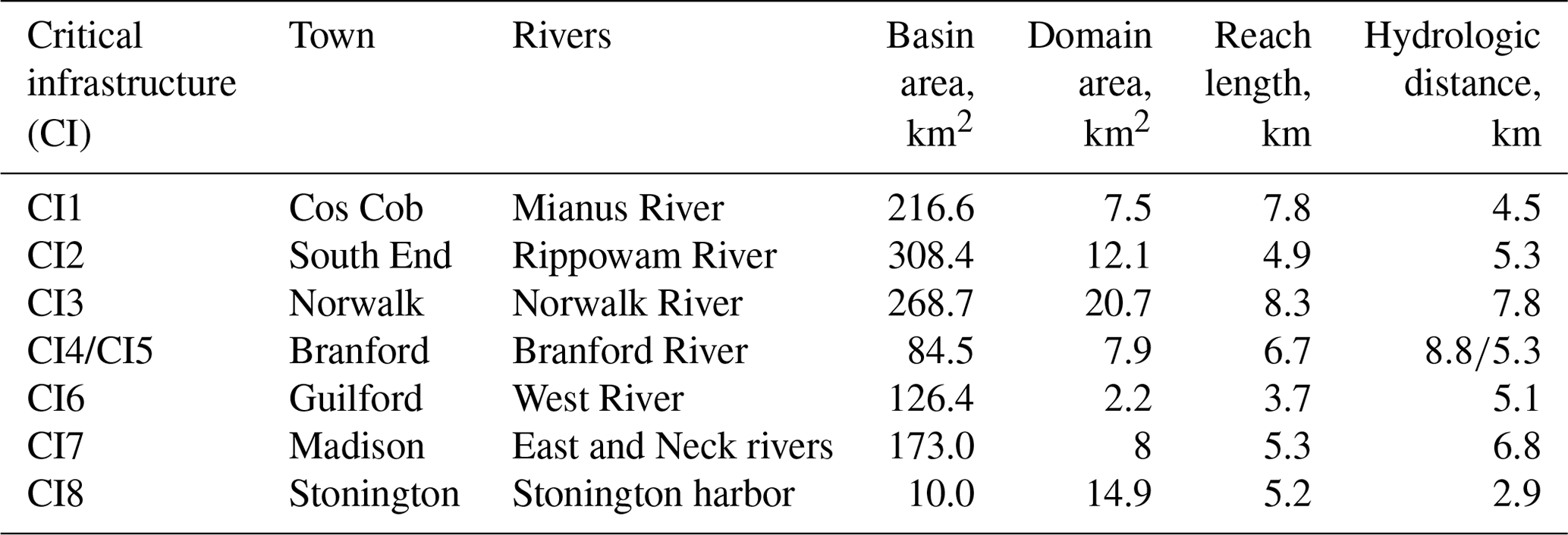
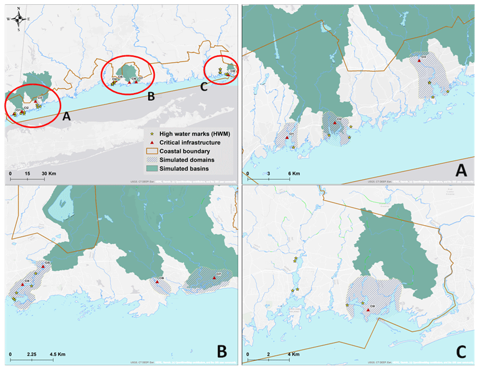
Figure 1Study area with associated watersheds and simulation domains. Locations of substations and USGS high-water marks are also shown. Red circles in the top left-hand panel and marked with A, B, and C are highlighted in panels (a) to (c), respectively. Background map by Esri web services, provided by UConn/CTDEEP, Esri, Garmin, USGS, NGA, EPA, USDA, and NPS.
For each river reach adjacent to a CI, we developed a hydrodynamic model domain, and we applied a distributed hydrological model for predicting river flows from the upstream river basin. Table 1 shows the specification of each river reach, associated drainage basin, the correspondent domain extent for the hydrodynamic simulations, and the hydrological distance (distance along the flow paths) of each power grid substation from the coastline. This distance was derived using the 30 m National Elevation Dataset (NED) for the continental United States (USGS, 2017).
Among the case study sites, two CIs are relatively inland (CI3 and CI4) (Table 1 – see hydrologic distance; Fig. 1 – see coastal boundary); nonetheless all the sites are included within the coastal area as defined by Connecticut General Statute (CGS) 22a-94(a) (https://www.cga.ct.gov/current/pub/chap_444.htm#sec_22a-94, last access: 28 January 2021). The considered rivers belong to watersheds ranging from 10 to 300 km2 in basin area, which are sub-basins of the Connecticut River basin. The hydrodynamic model simulation domains ranged from 3.7 to 8.3 km in river length and 2.2 to 20.7 km2 in area.
2.2 Simulation framework
To evaluate the effect of compound events, we selected four tropical storms: two actual hurricanes (Sandy and Irene) that hit Connecticut and two synthetic scenarios based on actual hurricanes Sandy and Florence. Both Irene (21–28 August 2011) and Sandy (22 October–2 November 2012) reached category 3, but they made landfall in Connecticut as category-1 hurricanes. The synthetic simulations (Sect. 2.2.1) include different atmospheric conditions leading to landfall scenarios with more significant impacts. The Sandy synthetic scenario represents Hurricane Sandy under future climate and sea surface conditions (Lackmann, 2015), while the synthetic scenarios for Florence were based on simulated surge-tide conditions and future SLR (see Sect. 2.2.1 and 2.3).
To investigate the flood characteristics considering the various scenarios, we devised a combined hydrological (Sect. 2.2.2) and hydrodynamic (Sect. 2.2.3) modeling framework (Fig. 2), forced with weather reanalysis and geospatial data for the actual events, and a numerical weather prediction model (Sect. 2.2.1) for the synthetic events (that is, synthetic Hurricane Florence and future Hurricane Sandy).
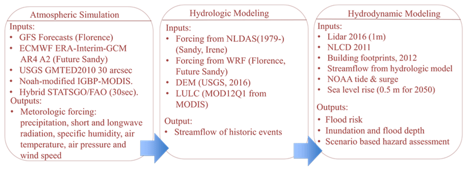
Figure 2Considered framework including atmospheric simulations and hydrologic and hydrodynamic modeling. Hurricane events (actual and simulated) and inputs and outputs of each component are shown. Readers should refer to Sect. 2.2 for specifications.
2.2.1 Atmospheric simulations
To simulate the two synthetic Sandy and Florence hurricane events, we used the Weather Research and Forecasting (WRF) system (Powers et al., 2017; Skamarock et al., 2008). For the synthetic Hurricane Florence event, we used a hurricane track forecast by the National Oceanic and Atmospheric Administration (NOAA) that, as of 6 September 2018, according to the Global Forecast System (GFS) forecasts of the National Centers for Environmental Prediction (NCEP), showed landfall on Long Island and in Connecticut on 14 September as a category-1 hurricane (Higgins et al., 2000).
We based synthetic Hurricane Sandy events on future climate conditions (post-2100).
For the soil type and texture input in the WRF model for both synthetic storm simulations, we used the USGS GMTED2010 30 arcsec (Danielson and Gesch, 2011) digital elevation model for the topography, the Noah-modified 21-category IGBP-MODIS (Friedl et al., 2010) for land use and vegetation input, and the hybrid STATSGO–FAO (30 s) (FAO-UNESCO, 1974, 1971–1981; FAO, 1991) for soil characteristics.
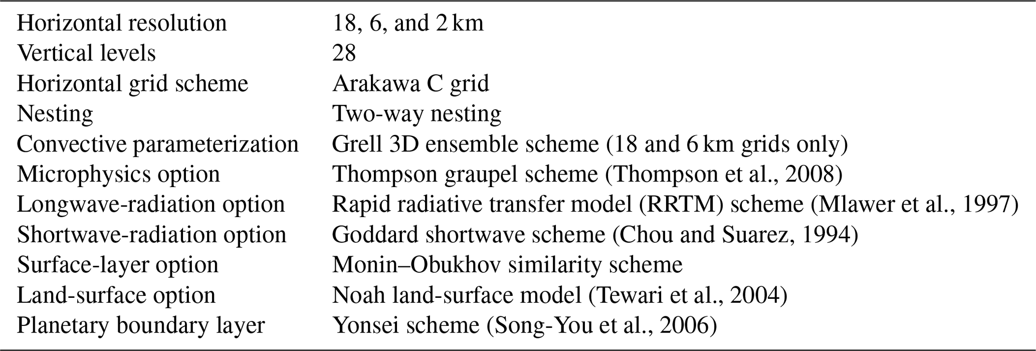
To simulate synthetic Hurricane Florence with WRF, we used the GFS forecasts at a spatial resolution as initial and boundary conditions. We used a three-grid setup with a coarse external domain of an 18 km spatial resolution and two nested domains with 6 and 2 km horizontal grid spacing, respectively. Two-way nesting was activated for both inner domains. Vertically, the domains stretched up to 50 mbar with 28 layers. We parameterized convective activity on the outer (resolution of 18 km) and the first nested (resolution of 6 km) domain using the Grell 3D ensemble scheme (Grell and Devenyi, 2002). Further details on the model setup are presented in Table 2.
For the future Hurricane Sandy scenario, we used the Hurricane Sandy simulations under future climate conditions (after 2100) by Lackman (2015), who used a three-grid setup at spatial resolutions of 54, 18, and 6 km. We defined initial and boundary conditions by altering the European Centre for Medium-Range Weather Forecasts (ECMWF) ERA-Interim reanalysis (Dee et al., 2011) data, based on five general circulation model (GCM)-projected, late-century thermodynamic changes derived from the IPCC (Intergovernmental Panel on Climate Change) AR4 A2 emissions scenario (Meehl et al., 2007). A complete description of the modeling framework is provided by Lackman (2015).
2.2.2 Hydrological modeling
To account for the river inflow (upstream boundary condition), we applied a physically based distributed hydrological model (CREST-SVAS (Coupled Routing and Excess Storage–Soil–Vegetation–Atmosphere–Snow)) described in Shen and Anagnostou (2017).
To simulate river discharges for the synthetic hurricanes (Florence and future Sandy), we used the WRF simulations at a 6 km and hourly spatiotemporal resolution, as described above. To force the hydrological model for the actual events (Sandy and Irene), we used data from Phase 2 of the North American Land Data Assimilation System (NLDAS-2) (Xia et al., 2012) dataset. NLDAS-2 is a gridded dataset derived from bias-corrected reanalysis and in situ observation data, with a 0.125∘ grid resolution and an hourly temporal resolution, available from 1 January 1979 to the present day. We derived the precipitation from daily rain gauge data over the continental United States, and all other forcing data came from the North American Regional Reanalysis (NARR) by NCEP (Higgins et al., 2000), to which we applied bias and vertical corrections. To reduce the computational effort, we performed the hydrological simulation using a hydrologically conditioned DEM at a 30 m spatial resolution (USGS, 2017).
The hydrologic simulation includes the use of land use and land cover information retrieved from the Moderate Resolution Imaging Spectroradiometer (“MOD12Q1” from MODIS) (Friedl and Sulla-Menashe, 2015). To compensate for the coarse resolution (500 m) of these data, we obtained imperviousness ratios using Connecticut's Changing Landscape (CCL) database and the National Land Cover Database (NLCD) at a 30 m resolution. In CREST-SVAS, the land-surface process was simulated by solving the coupled water and energy balances to generate streamflow at hourly time steps at the outlet of the studied watershed. CREST-SVAS was calibrated and validated for the whole Connecticut river basin (which contains all the investigated sites) with a Nash–Sutcliffe coefficient of efficiency (NSCE) of 0.63 (Shen and Anagnostou, 2017). We further validated the model considering hourly flows in two locations within the Housatonic River and Naugatuck River watersheds with an NSCE of 0.69 (Hardesty et al., 2018). The quality measures indicate a satisfactory model performance at the watershed scale over the topographic region that collectively includes our study sites.
2.2.3 Hydrodynamic modeling
To assess the flood hazard in terms of extent and the maximum depth of the flood, we implemented the Hydrologic Engineering Center's River Analysis System (HEC-RAS), developing two-dimensional model domains around the CI location. Except for CI4 and CI5, which are within the same simulation domain, each substation has an independent domain.
The inundation maps are derived using a 1 m lidar DEM (CtECO, 2016) taken as base maps for the study reaches. To better represent the impacts of urban establishments on inundation dynamics, urban features such as houses and buildings, which obstruct the flow of stormwater, were added to the bare-earth DEM. For this, we considered the building footprints from CtECO (2012) and identified positions of buildings and houses in the DEM by increasing the elevation of the pixels within the building footprint polygons by an arbitrary height of 4.5 m, assuming one-story buildings.
The considered locations have no bathymetric (underwater topography) data represented in the DEM. In general, the impact of inclusion or exclusion of bathymetry data on the hydrodynamic model simulations will vary according to the river size and event severity (Cook and Merwade, 2009). For the investigated events in this study, flood risk is mainly dominated by defense overflow. The proposed analysis focused upon the effects of extreme events that are so severe that all defenses would, in any case, be overtopped. This allows for a simplification of the modeling problem and for a correct approximation of flows even without detailed bathymetric information in the main channel, as underlined in Bates et al. (2005).
To reduce the computation time, we created a 2D mesh grid at a 10 m background resolution, enforced with break lines to intensify the riverbank and other areas with a large elevation gradient up to a 1 m resolution. CREST-SVAS provided the upstream boundary condition. National Water Level Observation Network (NWLON) data, provided by NOAA, offered the basis for defining the downstream boundary condition (coastal water level, including coastal tide, storm surge, and sea level). The latter data are available as actual observations and predictions at intervals of 6 min to 1 h. Figure 3 provides an example of one of the sites, showing the upstream and downstream boundaries, along with a map overlay of flooded areas of five (SD1–SD5) scenarios (see below) for CI2. We initiated the simulation with a warm-up period of 12 h to achieve stability. We chose the full momentum scheme in HEC-RAS and extracted hourly output from the simulation.
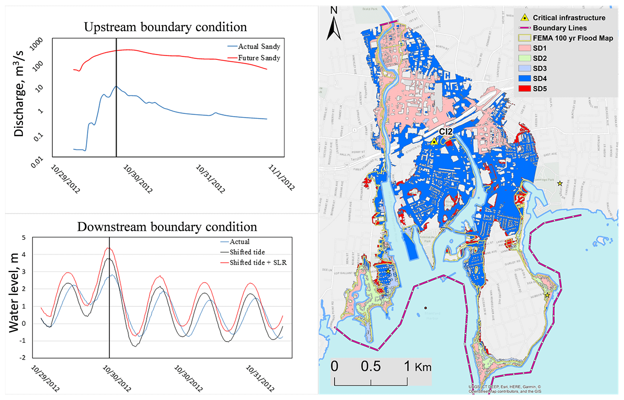
Figure 3Example of different scenarios showing the upstream boundary condition (top left-hand panel, including the discharge for actual Sandy and future Sandy) and downstream boundary (bottom left-hand panel, including tide, shifted tide, and shifted tide with SLR). Output flood extent is also shown (right-hand panel), including results for SD1 to SD5 (reader should refer to Table 3 and Sect. 2.2 for specification on the scenarios). Background map in the right-hand panel by Esri web services, provided by UConn/CTDEEP, Esri, Garmin, USGS, NGA, EPA, USDA, and NPS.
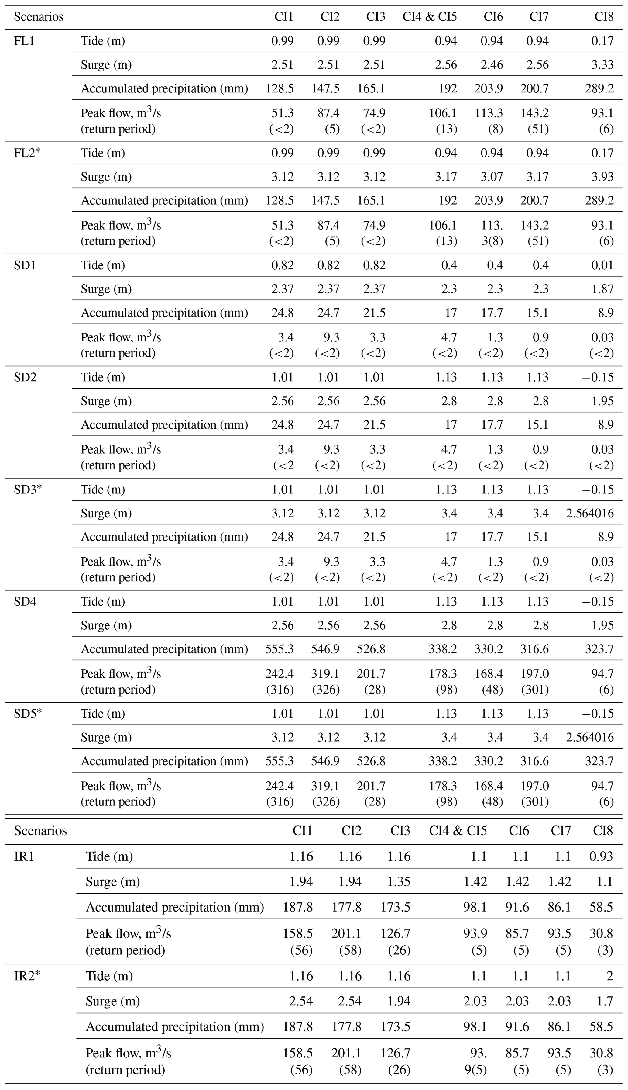
Table 3Peak tide and surge at the maximum total water-level instance; accumulated precipitation and peak flows (with return period reported within parentheses) for the simulated scenarios. The reader should refer to Sect. 2.2 for a detailed description of each hurricane scenario (IR for Irene, SD for Sandy, FL for Florence). The “*” denotes the scenarios having sea-level rise (SLR) added to the surge. Critical infrastructures are labeled CI1 to CI8 according to Table 1.
The model parameters were calibrated to obtain realistic water depths and extents, as compared to reference data collected for Sandy. To validate the hydrodynamic model simulations, we used surveyed HWMs (high-water marks) (Koenig et al., 2016) collected by the United States Geological Survey (USGS) after Hurricane Sandy at 15 selected locations spread across the simulation domains. HWMs are frequently used to calibrate and validate model outputs and satellite-based observations of flood depth (Bunya et al., 2010; Cañizares and Irish, 2008; Cariolet, 2010; Chang et al., 2007; Hostache et al., 2009; McEvoy et al., 2012; Pearson et al., 2018; Schumann et al., 2007a, b, 2008; Ziervogel et al., 2014). As for the flood extent, we further validated the model against the most accurate available information on the 2D extent and the maximum depth of storm surge for Sandy (FEMA, CT DEEP, 2013), created from field-verified HWMs and storm surge sensor data from the USGS.
An HWM does not necessarily indicate the maximum flood depth; rather, it can be a mark from a lower depth that lasts long enough to leave a trail. Based on this understanding, we compared the HWMs against the simulated flood depths within a 10×10 m radius around the high-water marks, also to avoid issues due to the presence of buildings in the DEM (boxplots in Fig. 4). The simulated depths demonstrated reasonable agreement with the collected HWM values (Fig. 4), with the model showing a slight overestimation. In this case, the systematic error fell within values of expected precision, implying a consistent positive bias in the simulations not strong enough to hinder the results.
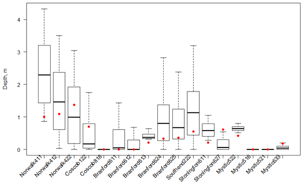
Figure 4Validation results (boxplot of water depth within 10×10 m around the high-water mark – HWM – location) compared to selected HWM (red dots) by USGS.
Figure 5 shows a visual comparison for CI1 and CI2 between the simulated inundation (Fig. 5a, c) and the reference extent (Fig. 5d, e). A slight overestimation of the flood level, ranging between 0.2 and 0.4 m, with a precision of 0.2 m or less, is observed for the inundation depths at the displayed locations, which is consistent with the results obtained locally, at the HWM locations (Fig. 4). Taking into consideration the accuracy of the inundation depth, the declared DEM accuracy (vertical RMSE ∼ 0.3 m), and the simplified modeling problem concerning bathymetry, the accuracy of the flood extent assessment was judged satisfactory.
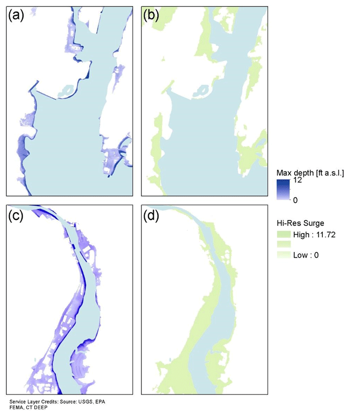
Figure 5Comparison between the results of the proposed model for two selected locations (a, c – CI1 and CI2, respectively) and the maximum surge extent as proposed by Connecticut Environmental Conditions Online (CT ECO) (c, d, respectively). Maximum depth ranges between 0 and 3.6 m a.s.l.
2.3 Compound scenarios
We modeled four types of synthetic compound-event scenarios, as well as actual events, by (1) simulating the synthetic hurricanes; (2) introducing a climate change factor, in the form of SLR (∼0.6 m), as projected for 2050, as a prediction for intermediate low probability (O'Donnell, 2017); (3) shifting the surge timing to make the surge peak level occur at local high tide; and (4) combining the SLR with the high-tide condition. The combination of these four event types yielded nine simulations, hereby coded as IR or SD for hurricanes Irene and Sandy and as FL for synthetic Hurricane Florence.
Two scenarios were created for Hurricane Irene. IR1 was actual Hurricane Irene that made landfall in Connecticut during high tide, and IR2 was the IR1 scenario with future SLR added to the tidal water level as a downstream boundary condition in HEC-RAS.
For Hurricane Sandy, we generated five scenarios. SD1 was actual Sandy. For SD2, we shifted the peak high tide to coincide with the maximum storm surge recorded, as derived from the local NOAA stations (hereafter referred to as “shifted-tide water levels”). We further added SLR to the shifted-tide water levels from SD2 to create the third scenario (SD3). The remaining two scenarios for Hurricane Sandy represented future climate conditions. Specifically, SD4 was the future hurricane scenario simulated with the GFS (Sect. 2.2.1) and shifted tidal water level. SD5 was future Sandy with shifted-tide water levels and SLR.
For the synthetic Hurricane Florence event, we simulated two scenarios. FL1 was the synthetic Florence event, based on the GFS track that gave landfall in Connecticut and Long Island (Sect. 2.2.1). FL2 was the same synthetic event, with SLR added to the coastal water levels.
Table 3 shows, for each scenario, the basin-averaged event accumulated precipitation (mm) and the simulated peak flow (m3/s) used as an upstream boundary condition in HEC-RAS, along with the recurrence interval of the peak flows derived using a log-Pearson probability distribution fitted using yearly maxima from the long-term simulated flows (1979–2019) from CREST. This shows how significant the precipitation forcing was for each considered scenario. For CI1, for example, the future Sandy (SD4 and SD5) scenario, with a peak flow of 242.4 m3/s, was the most extreme event with a recurrence interval of 316 years, followed by Irene (158.5 m3/s) and Florence (51.3 m3/s) with a recurrence interval of 56 and 2 years, respectively, whereas, for CI8, Florence and future Sandy had similar magnitudes with peak flows of 93.1 m3/s and 94.7 m3/s, respectively. In Table 3, we have summarized the maximum total water level (tide and surge) used in the model downstream of the study sites for all the scenarios. This Table represents the change in the severity of the coastal component of the compound scenarios concerning added challenges like shifted tide and SLR. For example, for CI3, the total water-level increases 1 m with the shifted tide (SD2 and SD4), and with SLR it becomes 4.4 m.
2.4 Compound-flood-hazard analysis
We investigated the compound effect of the different events by comparing flood area extents and flood depths for each event. For the flood area extent, we used as a baseline the 100-year flood maps provided by FEMA. We considered the distance correlation index (dCorr) (Székely et al., 2007) to identify the correlation of the differences between simulated and FEMA extent and compound events' parameters (flow and total water-level peak). dCorr values range from 0 to 1 expressing the dependence between two independent variables. The closer dCorr is to 1, the stronger the dependency would be, and zero implies that the two variables in question are statistically independent. dCorr can depict the non-monotonic associations of the variables and declare the dCorr value is zero if only the variables are statistically independent.
For the flood-level differences, we considered the overall distribution of water depths across the domain of the CI sites and investigated the time series of water depth at each location (Fig. 6 is an example of the simulated flood depth during the scenarios of Sandy (SD1–SD5) over time for CI2).
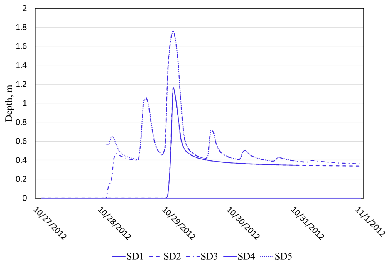
Figure 6Example of time series of depth values for the different scenarios of Sandy event at CI3 (SD1 to SD5, readers should refer to Table 3 and Sect. 2.4 for specification on the scenarios).
Table 4Overall extent of the inundated area (in km2), the relative difference (percent change in parentheses) compared to the FEMA 100-year flood zone and dCorr (correlation between differences in flood extent as compared to FEMA and flow and surge peak).
Note that minus values indicate area inundated less than FEMA's 100-year zone.
To evaluate the flood hazard in terms of flood depth, we computed a cumulative distribution function (CDF) to show the probability that the flood depth will attain a value less than or equal to each measured value. We estimated the CDF using all the depth values of all the grid of the simulation domain, for the time step when the inundation was maximal. We evaluated the depth empirical exceedance probability (Hanman et al., 2016; Lin et al., 2016; Warner and Tissot, 2012) within the whole domain, considering the maximum depth at each pixel, as suggested in Pasquier et al. (2019) and Hamman et al. (2016). The benefits of this empirical approach are that it overcomes sensitivity to the choice of the distribution and does not require a definition of the distribution parameters. By comparing the empirical distributions, we can investigate how changes in the scenario characteristics modify the frequency of the maximum inundation depths.
The study further looked at whether the depth of water at a station would change for various scenarios. Figure 6 shows an example of the flood depth over simulated time at CI3 for the scenarios of Sandy. We investigated pre-defined hazardous water levels for each station, as hypothetical values representing the height between the floor and the critical electric system in the station. Specifically, we considered 0.5, 1.5, and 2.5 m for threshold levels. As a measure of the potential threat to the electric infrastructure, we determined the percentage of time that the flood level was over each specific threshold (Fig. 9). These data were then used to assess potential flooding problems associated with on-site inundation: we associated the changes in risk posed to the CI from the different examined scenarios based on the changes in those percentages.
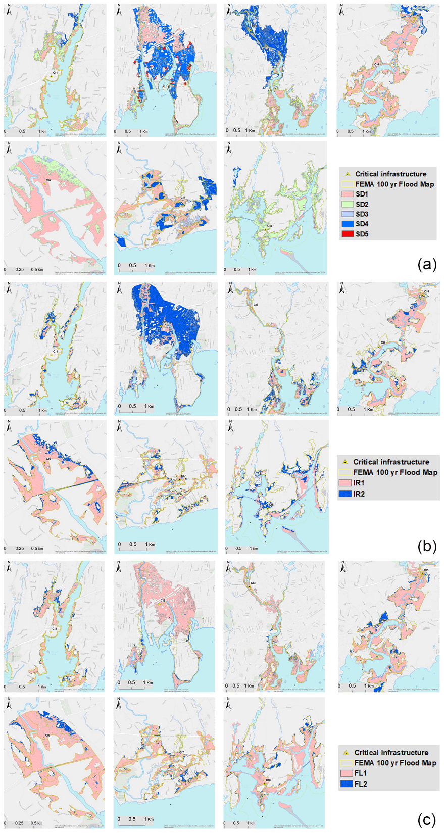
Figure 7Map overlay of maximum inundation for all the study domains containing CI1 through CI8 for the scenarios of Florence (FL1 and FL2; readers should refer to Table 3 and Sect. 2.2 for specification on the scenarios). Background map by Esri web services, provided by UConn/CTDEEP, Esri, Garmin, USGS, NGA, EPA, USDA, and NPS.
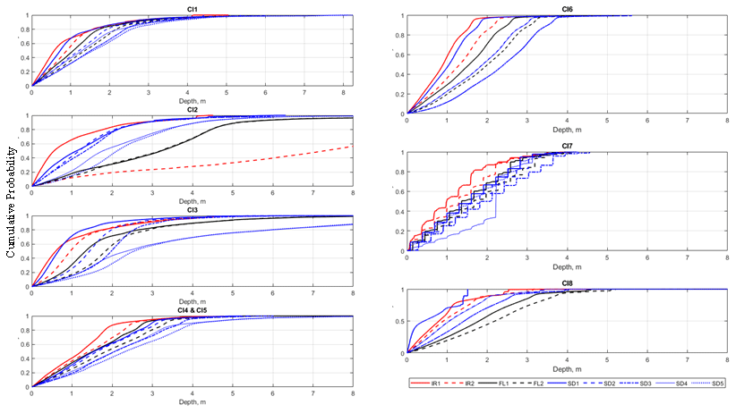
Figure 8Cumulative density plot of the depth of all the flooded cells during maximum inundation. Hurricanes scenarios are labeled according to Table 3 and explained in Sect. 2.2. Critical infrastructures are labeled CI1 to CI8, as described in Table 1.
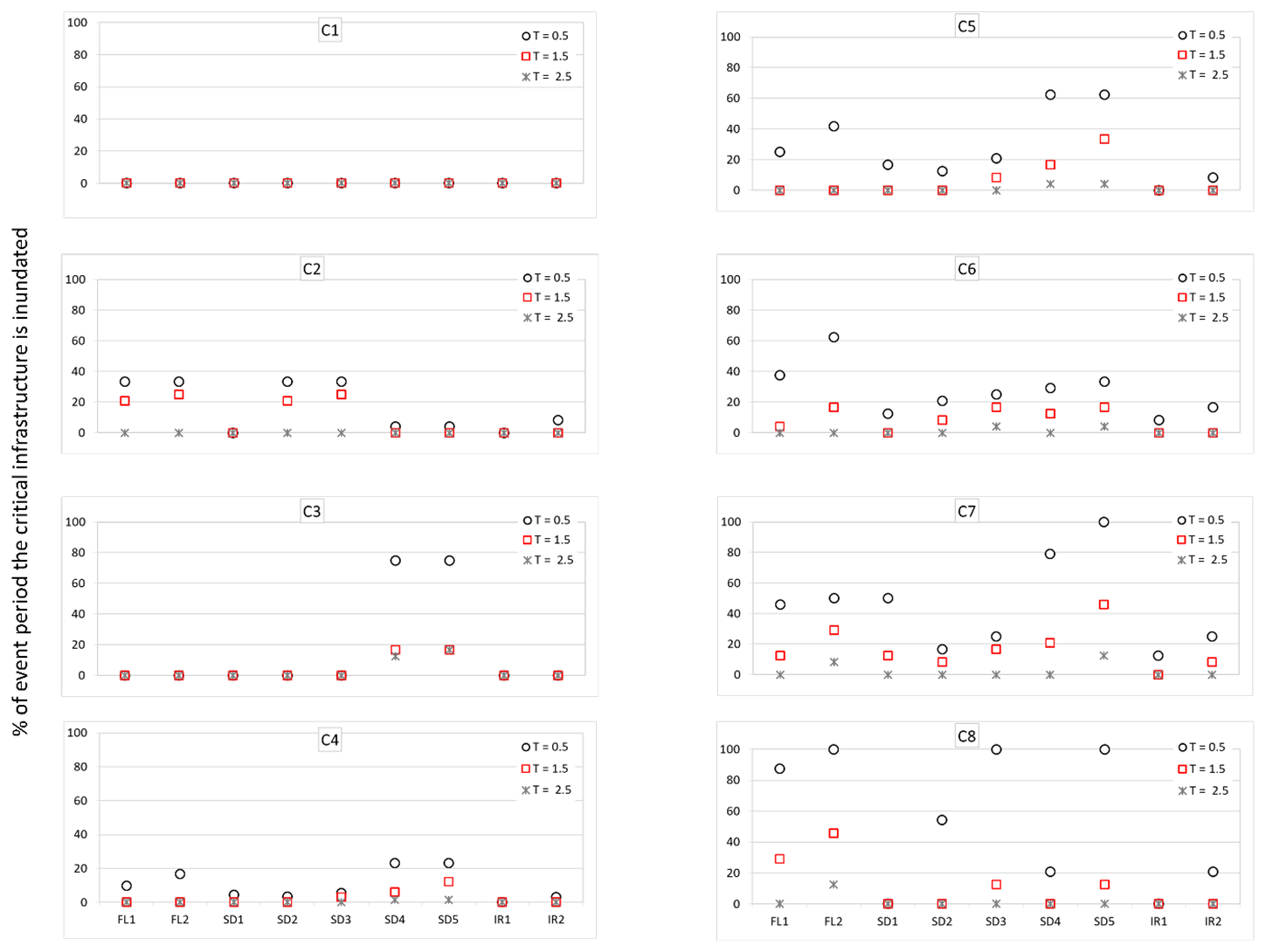
Figure 9Peak over threshold (T=0.5, 1.5, and 2.5 m) at selected critical infrastructures. Hurricanes scenarios, along the x axis, are labeled according to Table 3 and explained in Sect. 2.2. Critical infrastructures are labeled CI1 to CI8, as described in Table 1.
3.1 Flood extent
The inundation extents shown in Fig. 6 represent an aggregation of the overall runs rather than a specific simulation time, and the map represents the extent reached when all pixels had the maximum inundation depth. The total flood extent ranged between less than 1 km2 and more than 7 km2, with a minimum extent of 0.4 km2 for actual Sandy (SD1) at C8 and a maximum extent of 7.1 km2 for future Sandy (SD5) at C3. The results showed consistent agreement that the flood extent increased with increasing intensity of the event and an increase in the recurrence intervals of the flows (Table 3).
Changes across the study sites relative to the FEMA 100-year flood extent (Table 4, Fig. 7a–c) ranged from −87.8 % (for CI8 for SD1) to 192.2 % (for CI2 for IR2). Overall, the sites with a return period of less than 100 years showed consistently less flooding than those of the FEMA map, a finding best represented by the comparison of actual events, such as IR1.
Since the model performance shows a good agreement with the actual flood extent and the HWMs (Sect. 2.2.3), our results suggest that FEMA's flood maps do not fully capture the flood extent at least for some locations. Similar findings were reported in Jordi et al. (2019), Wang et al. (2014), and Xian et al. (2015), where tens-of-meter-scale absolute differences were found between the FEMA-estimated flood extents for Hurricane Sandy. The strength of correlation (dCorr) between changes in the upstream (flow peak) or downstream (surge peak) components and the absolute differences with the FEMA extent gives an idea of the importance of every single driver of change. For the cases investigated in this study, the percentage difference mostly depends on the surge: surge height explains more than 80 % of the variation in the differences to the FEMA extent (dCorr = 0.8 in median). CI6 appears to be the site where the surge has the strongest correlation with the absolute difference in flood extent, as compared to FEMA maps. The differences with FEMA maps are less related to the peak flows (median correlation 0.5, with maximum correlation recorded for CI3). As expected, the correlation with surge increases with the decrease in the hydrologic distance to the coast, while the correlation with the flow increases the further a site is from the coast, even though this relationship is not linear.
As we proceeded with the synthetic scenarios, adding compound and future climate, the results indicated the additional impacts of the joint flood drivers (shifted tide, surge, SLR).
For the same event, peak storm-tide levels occurring near local high tide (i.e., SD2) resulted in more flooding than those of events happening at low tide (like actual Sandy, SD1). Climate-change-related SLR exacerbated extreme event inundation relative to a fixed extent (FEMA) with variability that ranged from 8.3 % (CI4–CI5) to as high as 425 % (CI8). CI8 is the site hydrologically closer to the coast (see the hydrologic distance in Table 1), making it the most susceptible to the altered scenario. Nonetheless, the shifted tide also increased the inundation relative to the FEMA 100-year flood map for CI2 and CI4–CI5.
The effects of compound events emerged drastically with the combination of both shifted tide and SLR. Except for CI3 and CI8, all other CIs showed an increase in the percentage change from FEMA (Table 4). In comparison to SD1, SD3 exhibited increased inundation for all the CIs. The inundated area was about 146 % more (1.9 km2) for SD3 than SD1 (0.9 km2) for CI1, for example. The river flood peak for Hurricane Sandy had a recurrence interval of about 2 years, but the flood hazard associated with this event became more devastating if simulated in a compound way, including SLR and shifted tide. This result suggests that events of lower river flood severity (from fewer rain accumulations) can produce an aggravating impact, as the intensity of major storm surges increases due to shifted timing and SLR.
For synthetic Hurricane Florence and Hurricane Irene, we saw an increased flooded area in comparison to FEMA (Table 4); for CI2, for example, the increase was almost 200 % from IR1 to IR2. Again, this result confirms that accounting for river peak flow frequency alone does not effectively capture the severity of a flood hazard in the case of coastal locations.
For all the study sites for future Sandy, we saw consistent increases in flood extent (Table 4) from SD2 to SD4 and SD3 to SD5. Between SD2–SD3 and SD4–SD5, the only difference was the future projection of the flow. In comparison to the FEMA map, the percentage change ranged from −22.3 to +123.7. CI1, CI7, and CI8 for SD4 have less inundation than the FEMA 100-year map. This may be an indication of the significance of individual flood components specific to one site. For those sites, river flow might not be the most significant component of the flood. When we look at the hydrologic distances in Table 1, CI1 and CI8 are closer to the coastline, making them more prone to coastal flooding than fluvial flooding. When we looked at SD5 (which added SLR), all the sites except CI8 showed more flooding than the FEMA 100-year flood map. However CI8 had an increase of 22 % in inundation compared to SD4.
When we compare the worst-case future events (SD5 and IR2) to actual events (SD1 and IR1), we can see major changes in flood extents. The flood extent in all locations increased by about 60 % on average for future Sandy with both SLR and coinciding tide (SD5) in comparison to actual Sandy (SD1), with the highest impact in CI8 (+148 %). Looking at Irene, the worst-case future scenario (IR2) increased the flood extent by about 30 % on average for all locations compared to the actual event (IR2), with the highest impact in CI2 (101 %). Among all the events, Florence had the lowest expected changes between the current climate scenario (FL1) and the future one (FL2). One must note that Hurricane Florence had no actual impact in the study area; the simulation for this event was based on a hurricane track forecast by the GFS, which, if it materialized, would have produced a flood inundation of almost 5 km2 in CI3, and this extent could have increased by about 20 % in the worst-case future scenario (FL2) that includes shifted tide and SLR. Five of the CIs were outside the FEMA 100-year flood zone, but they present flooding for FL1 and SD3. For FL2 all of the study sites were more vulnerable (positive percent change), as compared to the FEMA map. Similar findings are presented for SD5, except for CI8.
3.2 Flood depths over the domain
While flooding occurs in all the presented scenarios, both extent and depth vary significantly between the different simulations. Depth is critical to consider while preparing for risk management as it is used in determining flood damage.
The CDFs of water depth for the whole domain (Fig. 8) confirm that the water depths derived for coupled events (i.e., high tide coinciding with surge peak or SLR and future climate) are generally higher than those derived from events with independent drivers. Note that for some cases (i.e., IR1 and IR2, for CI2 in Fig. 8) water depths increase very consistently as SLR increases. Large changes in the CDFs appear for lower water depths. Thus, regions with generally lower hazard (depth) will likely experience larger impacts under SLR. Results also confirm that scenarios with simultaneous high values for all these parameters implicated a higher vulnerability of the CIs. Comparing these changes in pairs (i.e., IR1 vs. IR2 or SD1 vs. SD3) also highlights that compound scenarios in the frequency of extreme values that go far beyond the average are much more pronounced than the related changes in the median depths (cumulative probability = 0.50). In particular, it may be asserted that more expressed changes in extremes could lead to corresponding “hazard shift” for all CIs, as represented in Fig. 8.
These results suggest that fluvial flow is not the only driver determining flood risk. Actual Irene (IR1) and synthetic Florence (FL) had higher river flood return periods than did actual Sandy (SD1) (Table 2). Nonetheless, the CDFs of the flood depth showed different behavior in terms of severity. For CI1, for example, IR1 had higher probabilities for lower depth, followed by SD1 and FL1. In CI8, SD1 had higher probabilities for lower values of depth. These findings highlight that neither the severity of rainfall nor the magnitude of river flow controls the flood characteristics, which are, instead, controlled by additional factors, such as storm surge, high tides, topography, and location of the site. CI7, for example, which is more coastal than the other CIs, presented increasing flood depth due to tidal timing.
As expected, and as previously highlighted when considering the flood extent (Table 4), climate played an important role in flood hazard changes. Furthermore, the effect of SLR was also evident for all the events (IR, SD, and FL), increasing the flood depth for the same exceedance probability. For CI6, for example, the 50 % exceedance corresponded to a ∼1 m depth of floodwater for IR1, increasing to ∼1.5 m for IR2. For the CI4 and CI5 sites, for an exceedance of 20 %, actual Irene produced ∼2 m of flood depth, whereas with SLR it was ∼2.5 m. Another way to put it is that, for CI4–CI5, IR1 had an exceedance of ∼20 % for a flood depth of 2 m, whereas IR2 had an increased exceedance level of 40 %. Similarly, for the 50% exceedance, FL1 and FL2 corresponded to a 1.5 and 2 m depth of floodwater, respectively, and we saw the trend for the Sandy event scenarios (SD2–SD3, SD4–SD5) as well.
This analysis highlighted that the timing of a storm is also crucial. The changes from SD1 to SD2 showed very well the impact of the shifted tide for all the sites. For CI3, for example, the 1 m flood depth had an exceedance of ∼88 % for SD2, whereas it was only ∼23 % for SD1.
Analysis of the overall flood depth across the whole domain shows that the coincidence of fluvial flood, high tide, and storm surge results in a significant increase in flood risk. SD3 and SD5 had all the components of a compound flood, and comparing them with SD1 gave us a clear idea of how severe a compound event can be in the future. CI3, for example, had exceedance levels of almost 30 %, 85 %, and 90 % for SD1, SD3, and SD5, respectively, for a flood depth of 1 m. This suggests the compound effect increases the intensity of the flood hazard.
3.3 Local risk for CI
Much of the flood damage in CI is incurred by components being submerged for a long period. Investigating the duration of the flood depth at the CI location (Fig. 9) should be considered in planning for any protective measures, such as elevating or waterproofing equipment. If a critical infrastructure shows 0 %, it means that for that scenario or event the water did not reach the substation at all, at least during the simulated timeframe. This could be due to the water flooding other upstream locations and therefore draining away from the station or because the topography of the landscape actually prevented water from reaching the area for some specific events.
According to our analysis, none of the scenarios has an actual impact on CI1. For the other CIs, comparing individual events we could see an increase in risk due to the compound hazard scenarios – that is, shifted tide and SLR. Important to note is that, for most of the sites, the compound risk due to SLR and tide timing was always higher for the lower water-level thresholds (0.5 m). This implies a higher risk for CI components currently positioned closer to the ground. Damage to the CI components is dictated by both the flood depth and the duration of submergence. The suggested high values of risk (increased percentage in inundation duration) (Fig. 9) further imply differences in the timing of repairs. In the cases of CI7 and CI8 (Fig. 9), the CIs remained submerged with 0.5 m of water for about 20 % of the event period for actual Sandy. For the worst-case future Sandy scenario, the location was flooded for more than 90 % of the event duration. This demonstrates the increased flood risk to which future climate conditions expose CI.
Another critical insight was provided by the Hurricane Florence scenarios. As mentioned earlier, Florence did not affect the study area, although an early GFS storm forecast track predicted landfall on Long Island and in Connecticut. For this event, the estimated measure of risk was about 20 %, and it was shown to increase to up to 40 % for the lower water depth (0.5 m) threshold in some locations. The result of the simulated scenario allows for an assessment of potential damage and for an identification of equipment that might be affected by future events under current climatic conditions. In this regard, comparing the results for the different CIs during the Sandy scenarios revealed an interesting pattern. While we might have expected a more significant impact over the whole domain when shifting the tide (Fig. 9, Table 3), we found different impacts in the CI locations. Notably, the risk appeared lower when the tides were shifted (Fig. 9) for some of the CIs (for example, CI5 and CI7). This can be explained by the fact that higher water levels in the domain were changing the water flows, allowing the flood to follow different drainable ways. This can be a very useful piece of information for deciding whether to and where to take measures in terms of flood occurrence and for potentially relocating CIs to avoid catastrophic compound flood events.
From Table 1 we can see that CI8 is the closest to the coastline followed by CI7, CI6, and CI5. From Fig. 9 we can see that all the CIs that are closer to the coastline are susceptible to changes in the downstream water-level condition (shifted tide and SLR) (Table 3). CI4 is the farthest from the coast followed by CI3. Both the CIs show a minimal response to changes in the coastal water level compared to CI5, CI6, and CI7. This analysis gives us conclusive evidence of risk associated with the location of the CI from the coastline.
Preparing for the challenges posed by climate change requires an understanding of current actual and possible, as well as future, scenarios of tropical storm impacts and a correct interpretation of the hazard imposed by compound flooding. In this work, we have developed and implemented a modeling framework that allows for addressing this task, focusing on coastal electric grid infrastructure (substations). To date, the design of these facilities typically has assumed the current climatic conditions. However, a changing climate, as well as the co-occurrence of compound drivers, and the resulting more extreme weather events mean those climate bands are becoming outdated, leaving infrastructure operating outside of its tolerance levels.
We explored a range of actual and synthetic hurricane scenarios, offering a system that could inform short- and long-term decisions. For the short-term decisions, the framework allowed us to investigate the characteristics of the hurricane-related inundation, considering the compound effect of riverine and coastal flooding coinciding, or not, with peak high tides. It allowed us to map those hazard–infrastructure intersections where risks will be likely exacerbated by climate change or compound events.
The results show that the vulnerability of each substation is linked to the event characteristics and how they vary depending on the distance from the coast – that is, inland substations are less affected by surge and SLR and more affected by rainfall accumulation events (such as Irene). While coastal areas are more vulnerable to CF, our analysis shows that significant impacts due to climate change can also be seen inland, for the increasing intensity of riverine events.
This study also highlights that, for some locations, FEMA maps significantly underestimate the actual flood risk, especially for CI in coastal areas. These maps generally fail to account for the impacts posed by simultaneous conditions, such as high tide and river flows, or for future climate impacts. This further suggests the need to develop improved criteria for recognizing the effects of existing and planned protection measurements, such as relocating equipment or CIs, where warranted.
Future research should consider improved estimation methods, including more detailed information on the variability in river properties (i.e., depth and width). Future works should also relate the frequency of inundation depths to return periods of precipitation, river flows, and surges, as well as differentiate among the individual effects of the components to determine the role of each in flooding impact.
Notwithstanding these challenges, the findings of this study highlight that, whenever possible, risk assessments across different critical locations directly or indirectly affecting critical infrastructure should be based on a consistent set of compound risks. This will ultimately allow for the building of resilience into different components of critical infrastructure to enable the system to function even under disaster conditions or to recover more quickly.
Considered software and models that are not in the public domain are available for research purposes upon request to the authors.
Data that are not in the public domain are available for research purposes upon request to the authors.
MKh, GS, XS, and EA conceived the study. XS and EA contributed to the conception of the hydrologic model. RL contributed to the production and analysis of the hydrologic model outputs. MKo and EN contributed to the analysis and interpretation of the climatic data. MKh and GS contributed to the automation of the hydraulic model and the interpretation of its results. All authors participated in drafting the article and revising it critically for important intellectual content. All authors gave the final approval of the published version.
The authors declare that they have no conflict of interest.
This work was supported by Eversource Energy.
This research has been supported by the Eversource Energy.
This paper was edited by Mauricio Gonzalez and reviewed by two anonymous referees.
Abii samra, N. and Henry, W.: Actions Before... and After a Flood, Power Energy Mag. IEEE, 9, 52–58, https://doi.org/10.1109/MPE.2010.939950, 2011.
Barnard, P. L., Erikson, L. H., Foxgrover, A. C., Hart, J. A. F., Limber, P., O'Neill, A. C., and Jones, J. M.: Dynamic flood modeling essential to assess the coastal impacts of climate change, Sci. Rep.-UK, 9, 4309, https://doi.org/10.1038/s41598-019-40742-z, 2019.
Bates, P. D., Dawson, R. J., Hall, J. W., Horritt, M. S., Nicholls, R. J., Wicks, J., and Ali Mohamed Hassan, M. A.: Simplified two-dimensional numerical modelling of coastal flooding and example applications, Coast. Eng., 52, 793–810, https://doi.org/10.1016/j.coastaleng.2005.06.001, 2005.
Bevacqua, E., Maraun, D., Vousdoukas, M. I., Voukouvalas, E., Vrac, M., Mentaschi, L., and Widmann, M.: Higher probability of compound flooding from precipitation and storm surge in Europe under anthropogenic climate change, Sci. Adv., 5, eaaw5531, https://doi.org/10.1126/sciadv.aaw5531, 2019.
Blöschl, G., Hall, J., Parajka, J., Perdigão, R. A. P., Merz, B., Arheimer, B., Aronica, G. T., Bilibashi, A., Bonacci, O., Borga, M., Čanjevac, I., Castellarin, A., Chirico, G. B., Claps, P., Fiala, K., Frolova, N., Gorbachova, L., Gül, A., Hannaford, J., Harrigan, S., Kireeva, M., Kiss, A., Kjeldsen, T. R., Kohnová, S., Koskela, J. J., Ledvinka, O., Macdonald, N., Mavrova-Guirguinova, M., Mediero, L., Merz, R., Molnar, P., Montanari, A., Murphy, C., Osuch, M., Ovcharuk, V., Radevski, I., Rogger, M., Salinas, J. L., Sauquet, E., Šraj, M., Szolgay, J., Viglione, A., Volpi, E., Wilson, D., Zaimi, K., and Živković, N.: Changing climate shifts timing of European floods, Science, 80, 588–590, https://doi.org/10.1126/science.aan2506, 2017.
Bunya, S., Dietrich, J. C., Westerink, J. J., Ebersole, B. A., Smith, J. M., Atkinson, J. H., and Roberts, H. J.: A High-Resolution Coupled Riverine Flow, Tide, Wind, Wind Wave, and Storm Surge Model for Southern Louisiana and Mississippi. Part I: Model Development and Validation, Mon. Weather Rev., 138, 345–377. https://doi.org/10.1175/2009MWR2906.1, 2010.
Cañizares, R. and Irish, J. L.: Simulation of storm-induced barrier island morphodynamics and flooding, Coast. Eng., 55, 1089–1101, https://doi.org/10.1016/J.COASTALENG.2008.04.006, 2008.
Cariolet, J.-M.: Use of high water marks and eyewitness accounts to delineate flooded coastal areas: The case of Storm Johanna (10 March 2008) in Brittany, France, Ocean Coast. Manag., 53, 679–690, https://doi.org/10.1016/J.OCECOAMAN.2010.09.002, 2010.
Chang, S. E., McDaniels, T. L., Mikawoz, J., and Peterson, K.: Infrastructure failure interdependencies in extreme events: power outage consequences in the 1998 Ice Storm, Nat. Hazards, 41, 337–358, https://doi.org/10.1007/s11069-006-9039-4, 2007.
Chou, M.-D. and Suarez, M. J.: An Efficient Thermal Infrared Radiation Parameterization for Use in General Circulation Models, NASA Technical Memorandum 104606(3)85, available at: https://archive.org/details/nasa_techdoc_19950009331 (last access: 9 February 2021), 1994.
Cook, A. and Merwade, V.: Effect of topographic data, geometric configuration and modeling approach on flood inundation mapping, J. Hydrol., 377, 131–142, https://doi.org/10.1016/j.jhydrol.2009.08.015, 2009.
Crossett, K., Ache, B., Pacheco, P., and Haber, K.: National Coastal Population Report: Population Trends from 1970 to 2020, Silver Spring, MD, available at: https://coast.noaa.gov/digitalcoast/training/population-report.html (last access: 9 February 2021), 2013.
CtECO: 2012 Impervious Surface Download, available at: http://www.cteco.uconn.edu/projects/ms4/impervious2012.htm (last access: 29 January 2021), 2012.
CtECO: Connecticut Elevation (Lidar) Data, available at: http://www.cteco.uconn.edu/data/lidar/index.htm (last access: 29 January 2021), 2016.
Danielson, J. J. and Gesch, D. B.: Global multi-resolution terrain elevation data 2010 (GMTED2010), U.S. Geological Survey Open-File Report 2011–1073, 26 p., 2011.
Dawson, R. J., Thompson, D., Johns, D., Wood, R., Darch, G., Chapman, L., Hughes, P. N., Watson, G. V. R., Paulson, K., Bell, S., Gosling, S. N., Powrie, W., and Hall, J. W.: A systems framework for national assessment of climate risks to infrastructure, Philos. Trans. R. Soc. A Math. Phys. Eng. Sci., 376, https://doi.org/10.1098/rsta.2017.0298, 2018.
de Bruijn, K. M., Maran, C., Zygnerski, M., Jurado, J., Burzel, A., Jeuken, C., and Obeysekera, J.: Flood Resilience of Critical Infrastructure: Approach and Method Applied to Fort Lauderdale, Florida, Water, 11, https://doi.org/10.3390/w11030517, 2019.
de Bruijn, K., Buurman, J., Mens, M., Dahm, R., and Klijn, F.: Resilience in practice: Five principles to enable societies to cope with extreme weather events, Environ. Sci. Policy, 70, 21–30, https://doi.org/10.1016/j.envsci.2017.02.001, 2017.
Dee, D. P., Uppala, S. M., Simmons, A. J., Berrisford, P., Poli, P., Kobayashi, S., Andrae, U., Balmaseda, M. A., Balsamo, G., Bauer, P., Bechtold, P., Beljaars, A. C. M., van de Berg, L., Bidlot, J., Bormann, N., Delsol, C., Dragani, R., Fuentes, M., Geer, A. J., Haimberger, L., Healy, S. B., Hersbach, H., Hólm, E. V., Isaksen, L., Kållberg, P., Köhler, M., Matricardi, M., McNally, A. P., Monge-Sanz, B. M., Morcrette, J.-J., Park, B.-K., Peubey, C., de Rosnay, P., Tavolato, C., Thépaut, J.-N., and Vitart, F.: The ERA-Interim reanalysis: Configuration and performance of the data assimilation system, Q. J. Roy. Meteor. Soc., 137, 553–597, https://doi.org/10.1002/qj.828, 2011.
Dottori, F., Szewczyk, W., Ciscar, J. C., Zhao, F., Alfieri, L., Hirabayashi, Y., Bianchi, A., Mongelli, I., Frieler, K., Betts, R. A., and Feyen, L.: Increased human and economic losses from river flooding with anthropogenic warming, Nat. Clim. Change, 8, 781–786, https://doi.org/10.1038/s41558-018-0257-z, 2018.
FAO: The digitized soil map of the world, World Soil Resource Rep. 67, FAO, Rome, 1991.
Food and Agriculture Organization of the United Nations - United Nations Educational, Scientific and Cultural Organization (FAO-UNESCO): Soil Map of the World (1:5 000 000), vol. 1 legend, UNESCO, Paris, France, 1974.
Food and Agriculture Organization of the United Nations - United Nations Educational, Scientific and Cultural Organization (FAO-UNESCO): Soil Map of the World (1:5 000 000), vol. 1–10, UNESCO, Paris, France, 1971–1981.
FEMA, CT DEEP: Coastal Hazards Map Viewer Information, available at: https://cteco.uconn.edu/viewer/index.html?viewer=coastalhazards (last access: 29 January 2021), 2013.
FEMA: Reducing Flood Effects in Critical Facilities. HSFE60-13-0002, 0003 / April 2013, available at: http://core-es.com/wp-content/uploads/FEMA-RA2-Reducing-Flood-Effects-in-Critical-Facilities.pdf (last access 29 January 2021), 2013.
Friedl, M. and Sulla-Menashe, D.: MCD12Q1 MODIS/Terra+Aqua Land Cover Type Yearly L3 Global 500m SIN Grid V006. NASA EOSDIS Land Processes DAAC, https://doi.org/10.5067/MODIS/MCD12Q1.006, 2015.
Friedl, M. A., Sulla-Menashe, D., Tan, B., Schneider, A., Ramankutty, N., Sibley, A., and Huang, X.: MODIS Collection 5 global land cover: Algorithm refinements and characterization of new datasets, Remote Sens. Environ., 114, 168–182, https://doi.org/10.1016/j.rse.2009.08.016, 2010.
Grell, G. A. and Dévényi, D.: A generalized approach to parameterizing convection combining ensemble and data assimilation techniques, Geophys. Res. Lett., 29, 34–38, https://doi.org/10.1029/2002GL015311, 2002.
Hallegatte, S., Green, C., Nicholls, R. J., and Corfee-Morlot, J.: Future flood losses in major coastal cities, Nat. Clim. Change, 3, 802–806, https://doi.org/10.1038/nclimate1979, 2013.
Hamman, J. J., Hamlet, A. F., Lee, S.-Y., Fuller, R., and Grossman, E. E.: Combined Effects of Projected Sea Level Rise, Storm Surge, and Peak River Flows on Water Levels in the Skagit Floodplain, Northwest Sci., 90, 57–78, https://doi.org/10.3955/046.090.0106, 2016.
Hardesty, S., Shen, X., Nikolopoulos, E., and Anagnostou, E.: A Numerical Framework for Evaluating Flood Inundation Hazard under Different Dam Operation Scenarios–A Case Study in Naugatuck River, Water-Sui., 10, 1798, https://doi.org/10.3390/w10121798, 2018.
Higgins, W., Shi, W., Yarosh, E., and Joyce, R.: Improved United States precipitation quality control system and analysis, NCEP/Climate Prediction Center ATLAS No. 7, 40 pp., 2000.
Hostache, R., Matgen, P., Schumann, G., Puech, C., Hoffmann, L., and Pfister, L.: Water Level Estimation and Reduction of Hydraulic Model Calibration Uncertainties Using Satellite SAR Images of Floods, IEEE T. Geosci. Remote S., 47, 431–441, https://doi.org/10.1109/TGRS.2008.2008718, 2009.
Jordi, A., Georgas, N., Blumberg, A., Yin, L., Chen, Z., Wang, Y., Schulte, J., Ramaswamy, V., Runnels, D., and Saleh, F.: A next-generation coastal ocean operational system, B. Am. Meteorol. Soc., 100, 41–53, https://doi.org/10.1175/BAMS-D-17-0309.1, 2019.
Karagiannis, G. M., Chondrogiannis, S., Krausmann, E., and Turksezer, Z. I.: Power grid recovery after natural hazard impact, EUR 28844 EN, https://doi.org/10.2760/87402, European Commission, Luxembourg, 2017.
Koenig, T. A., Bruce, J. L., O’Connor, J., McGee, B. D., Holmes Jr., R. R., Hollins, R., Forbes, B. T., Kohn, M. S., Schellekens, M., Martin, Z. W., and Peppler, M. C.: Identifying and preserving high-water mark data, U.S. Geological Survey, Reston, VA., https://doi.org/10.3133/tm3A24, 2016.
Kwasinski, W. W. Weaver, P. L. Chapman, and P. T. Krein: “Telecommunications Power Plant Damage Assessment for Hurricane Katrina – Site Survey and Follow-Up Results”, IEEE Syst J., 3, 277–287, 2009.
Lackmann, G. M.: Hurricane Sandy before 1900, and after 2100, B. Am. Meteorol. Soc., 96, 547–560, https://doi.org/10.1175/BAMS-D-14-00123.1, 2015.
Leonard, M., Westra, S., Phatak, A., Lambert, M., Van Den Hurk, B., Mcinnes, K., and Stafford-Smith, M.: A compound event framework for understanding extreme impacts, WIRES Clim. Change, 5, 113–128, https://doi.org/10.1002/wcc.252, 2014.
Lin, N., Kopp, R. E., Horton, B. P., and Donnelly, J. P.: Hurricane Sandy's flood frequency increasing from year 1800 to 2100, P. Natl. Acad. Sci. USA, 113, 12071–12075, https://doi.org/10.1073/pnas.1604386113, 2016.
Marsooli, R., Lin, N., Emanuel, K., and Feng, K.: Climate change exacerbates hurricane flood hazards along US Atlantic and Gulf Coasts in spatially varying patterns, Nat. Commun., 10, https://doi.org/10.1038/s41467-019-11755-z, 2019.
McEvoy, D., Ahmed, I., and Mullett, J.: The impact of the 2009 heat wave on Melbourne's critical infrastructure, Local Environ., 17, 783–796, https://doi.org/10.1080/13549839.2012.678320, 2012.
Meehl, G. A., Covey, C., Delworth, T., Latif, M., McAvaney, B., Mitchell, J. F. B., Stouffer, R. J., and Taylor, K. E.: The WCRP CMIP3 multimodel dataset: A new era in climatic change research, B. Am. Meteorol. Soc., 88, 1383–1394, https://doi.org/10.1175/BAMS-88-9-1383, 2007.
Mlawer, E. J., Taubman, S. J., Brown, P. D., Iacono, M. J., and Clough, S. A.: Radiative transfer for inhomogeneous atmospheres: RRTM, a validated correlated–k model for the longwave, J. Geophys. Res., 102, 16663–16682. https://doi.org/10.1029/97JD00237, 1997.
Moftakhari, H. R., Salvadori, G., Agha Kouchak, A., Sanders, B. F., and Matthew, R. A.: Compounding effects of sea level rise and fluvial flooding, P. Natl. Acad. Sci. USA, 114, 9785–9790. https://doi.org/10.1073/pnas.1620325114, 2017.
Muis, S., Verlaan, M., Winsemius, H. C., Aerts, J. C. J. H., and Ward, P. J.: A global reanalysis of storm surges and extreme sea levels, Nat. Commun., 7, 11969, https://doi.org/10.1038/ncomms11969, 2016.
O'Donnell, J.: Sea Level Rise Connecticut Final Report, available at: https://circa.uconn.edu/wp-content/uploads/sites/1618/2019/02/SeaLevelRiseConnecticut-Final-Report.pdf (last access: 10 January 2020), 2017.
Pant, R., Thacker, S., Hall, J. W., Alderson, D., and Barr, S.: Critical infrastructure impact assessment due to flood exposure, J. Flood Risk Manag., 11, 22–33, https://doi.org/10.1111/jfr3.12288, 2018.
Pasquier, U., He, Y., Hooton, S., Goulden, M., and Hiscock, K. M.: An integrated 1D–2D hydraulic modelling approach to assess the sensitivity of a coastal region to compound flooding hazard under climate change, Nat. Hazards, 98, 915–937, https://doi.org/10.1007/s11069-018-3462-1, 2019.
Pearson, J., Punzo, G., Mayfield, M., Brighty, G., Parsons, A., Collins, P., Jeavons, S., and Tagg, A.: Flood resilience: consolidating knowledge between and within critical infrastructure sectors, Environ. Syst. Decis., 38, 318–329, https://doi.org/10.1007/s10669-018-9709-2, 2018.
Powers, J. G., Klemp, J. B., Skamarock, W. C., Davis, C. A., Dudhia, J., Gill, D. O., Coen, J. L., and Gochis, D. J.: The Weather Research and Forecasting Model: Overview, system efforts, and future directions, B. Am. Meteorol. Soc., 98, 1717–1737, https://doi.org/10.1175/BAMS-D-15-00308.1, 2017.
Quinn, N., Bates, P. D., Neal, J., Smith, A., Wing, O., Sampson, C., Smith, J., and Heffernan, J.: The Spatial Dependence of Flood Hazard and Risk in the United States, Water Resour. Res., 55, 1890–1911, https://doi.org/10.1029/2018WR024205, 2019.
Schumann, G., Hostache, R., Puech, C., Hoffmann, L., Matgen, P., Pappenberger, F., and Pfister, L.: High-Resolution 3-D Flood Information From Radar Imagery for Flood Hazard Management, IEEE T. Geosci. Remote S., 45, 1715–1725, https://doi.org/10.1109/TGRS.2006.888103, 2007a.
Schumann, G., Matgen, P., Cutler, M. E. J., Black, A., Hoffmann, L., and Pfister, L.: Comparison of remotely sensed water stages from LiDAR, topographic contours and SRTM, ISPRS J. Photogramm., 63, 283–296. https://doi.org/10.1016/J.ISPRSJPRS.2007.09.004, 2008.
Schumann, G., Matgen, P., Hoffmann, L., Hostache, R., Pappenberger, F., and Pfister, L.: Deriving distributed roughness values from satellite radar data for flood inundation modelling, J. Hydrol., 344, 96–111, https://doi.org/10.1016/J.JHYDROL.2007.06.024, 2007b.
Reed, D. A., Powell, M. D., and Westerman, J. M.: Energy Supply System Performance for Hurricane Katrina, J. Energy Eng., 136, 95–102, https://doi.org/10.1061/(ASCE)EY.1943-7897.0000028, 2010.
Shen, X. and Anagnostou, E. N.: A framework to improve hyper-resolution hydrological simulation in snow-affected regions, J. Hydrol., 552, 1–12, https://doi.org/10.1016/j.jhydrol.2017.05.048, 2017.
Skamarock, W. C., Klemp, J. B., Dudhia, J., Gill, D. O., Barker, D. M., Duda, M. G., Huang, X., Wang, W., and Powers, J. G.: A Description of the Advanced Research WRF Version 3 (No. NCAR/TN-475+STR), University Corporation for Atmospheric Research, National Center for Atmospheric Research Boulder, Colorado, USA, https://doi.org/10.5065/D68S4MVH, 2008.
Song-You, H., Noh, Y., and Dudhia, J.: A new vertical diffusion package with an explicit treatment of entrainment processes, Mon. Weather Rev., 134, 2318–2341, https://doi.org/10.1175/MWR3199.1, 2006.
Székely, G. J., Rizzo, M. L., and Bakirov, N. K.: Measuring and testing dependence by correlation of distances, Ann. Stat., 35, 2769–2794, https://doi.org/10.1214/009053607000000505, 2007.
Tewari, M. F., Chen, W., Wang, J., Dudhia, M. A., LeMone, K., Mitchell, M. E., Gayno, G., Wegiel, J., and Cuenca, R. H.: Implementation and verification of the unified NOAH land surface model in the WRF model, 20th conference on weather analysis and forecasting/16th conference on numerical weather prediction (formerly paper number 17.5), 11–15, available at: https://ams.confex.com/ams/84Annual/techprogram/paper_69061.htm (last access: 9 February 2021), 2004.
Thompson, G., Paul, R. F., Roy, M. R., and William, D. H.: Explicit Forecasts of Winter Precipitation Using an Improved Bulk Microphysics Scheme. Part II: Implementation of a New Snow Parameterization, Mon. Weather Rev., 136, 5095–5115, https://doi.org/10.1175/2008MWR2387.1, 2008.
United States Geological Survey (USGS): 1/9th Arc-second Digital Elevation Models (DEMs) – USGS National Map 3DEP Downloadable Data Collection, United States Geological Survey, available at: https://catalog.data.gov/dataset/usgs-national-elevation-dataset-ned (last access: February 2021), 2017.
Vousdoukas, M. I., Mentaschi, L., Voukouvalas, E., Verlaan, M., Jevrejeva, S., Jackson, L. P., and Feyen, L.: Global probabilistic projections of extreme sea levels show intensification of coastal flood hazard, Nat. Commun., 9, 1–12, https://doi.org/10.1038/s41467-018-04692-w, 2018.
Wahl, T., Jain, S., Bender, J., Meyers, S. D., and Luther, M. E.: Increasing risk of compound flooding from storm surge and rainfall for major US cities, Nat. Clim. Change, 5, 1093–1097, https://doi.org/10.1038/nclimate2736, 2015.
Wang, H., Loftis, J., Liu, Z., Forrest, D., and Zhang, J.: The Storm Surge and Sub-Grid Inundation Modeling in New York City during Hurricane Sandy, J. Mar. Sci. Eng., 2, 226–246, https://doi.org/10.3390/jmse2010226, 2014.
Warner, N. N. and Tissot, P. E.: Storm flooding sensitivity to sea level rise for Galveston Bay, Texas, Ocean Eng., 44, 23–32, https://doi.org/10.1016/J.OCEANENG.2012.01.011, 2012.
Winsemius, H. C., Van Beek, L. P. H., Jongman, B., Ward, P. J., and Bouwman, A.: A framework for global river flood risk assessments, Hydrol. Earth Syst. Sci., 17, 1871–1892, https://doi.org/10.5194/hess-17-1871-2013, 2013.
Xia, Y., Mitchell, K., Ek, M., Sheffield, J., Cosgrove, B., Wood, E., Luo, L., Alonge, C., Wei, H., Meng, J., Livneh, B., Lettenmaier, D., Koren, V., Duan, Q., Mo, K., Fan, Y., and Mocko, D.: Continental-scale water and energy flux analysis and validation for the North American Land Data Assimilation System project phase 2 (NLDAS-2): 1. Intercomparison and application of model products, J. Geophys. Res.-Atmos., 117, https://doi.org/10.1029/2011JD016048, 2012.
Xian, S., Lin, N., and Hatzikyriakou, A.: Storm surge damage to residential areas: a quantitative analysis for Hurricane Sandy in comparison with FEMA flood map, Nat. Hazards, 79, 1867–1888, https://doi.org/10.1007/s11069-015-1937-x, 2015.
Ziervogel, G., New, M., Archer van Garderen, E., Midgley, G., Taylor, A., Hamann, R., Stuart-Hill, S., Myers, J., and Warburton, M.: Climate change impacts and adaptation in South Africa, WIRES Clim. Change, 5, 605–620. https://doi.org/10.1002/wcc.295 , 2014.
Zscheischler, J., Westra, S., van den Hurk, B. J. J. M., Seneviratne, S. I., Ward, P. J., Pitman, A., and Zhang, X.: Future climate risk from compound events, Nat. Clim. Change, 8, 469–477, https://doi.org/10.1038/s41558-018-0156-3, 2018.