Investigating causal factors of shallow landslides in grassland regions of Switzerland

Mountainous grassland slopes can be severely affected by soil erosion, among which shallow landslides are a crucial process, indicating instability of slopes. We determine the locations of shallow landslides across different sites to better understand regional differences and to identify their triggering causal factors. Ten sites across Switzerland located in the Alps (eight sites), in foothill regions (one site) and the Jura Mountains (one site) were selected for statistical evaluations. For the shallow-landslide inventory, we used aerial images (0.25 m) with a deep learning approach (U-Net) to map the locations of eroded sites. We used logistic regression with a group lasso variable selection method to identify important explanatory variables for predicting the mapped shallow landslides. The set of variables consists of traditional susceptibility modelling factors and climate-related factors to represent local as well as cross-regional conditions. This set of explanatory variables (predictors) are used to develop individual-site models (local evaluation) as well as an all-in-one model (cross-regional evaluation) using all shallow-landslide points simultaneously. While the local conditions of the 10 sites lead to different variable selections, consistently slope and aspect were selected as the essential explanatory variables of shallow-landslide susceptibility. Accuracy scores range between 70.2 % and 79.8 % for individual site models. The all-in-one model confirms these findings by selecting slope, aspect and roughness as the most important explanatory variables (accuracy = 72.3 %). Our findings suggest that traditional susceptibility variables describing geomorphological and geological conditions yield satisfactory results for all tested regions. However, for two sites with lower model accuracy, important processes may be under-represented with the available explanatory variables. The regression models for sites with an east–west-oriented valley axis performed slightly better than models for north–south-oriented valleys, which may be due to the influence of exposition-related processes. Additionally, model performance is higher for alpine sites, suggesting that core explanatory variables are understood for these areas.

1 Introduction

Soil erosion is an issue affecting many regions of the world and can have severe consequences for the environment and humanity (e.g. water pollution or food production) (Pimentel et al., 1995; Pimentel and Burgess, 2013; O'Mara, 2012; Alewell et al., 2009, 2020). In Switzerland, grasslands of mountain and hill slopes can be strongly affected by soil erosion, which can be caused by natural (e.g. precipitation events) and anthropogenic processes (e.g. land-use management) (Tasser et al., 2003; Meusburger and Alewell, 2008; Zweifel et al., 2019; Geitner et al., 2021; Lepeška, 2016). The most visible form of erosion in grassland soils showing bare soil areas can be categorised as shallow erosion (Geitner et al., 2021) (Fig. 1). These shallow-erosion sites are mainly triggered by prolonged and intense rainfall events (shallow landslides) or through abrasion by snow (snow gliding, avalanches) (Wiegand and Geitner, 2010; Geitner et al., 2021). However, in many cases, a combination of these processes can lead to shallow-erosion sites, and triggering processes cannot be distinguished from aerial photos. Therefore, we use the term shallow landslides in our regions and the frame of this study with no implication of the triggering event.

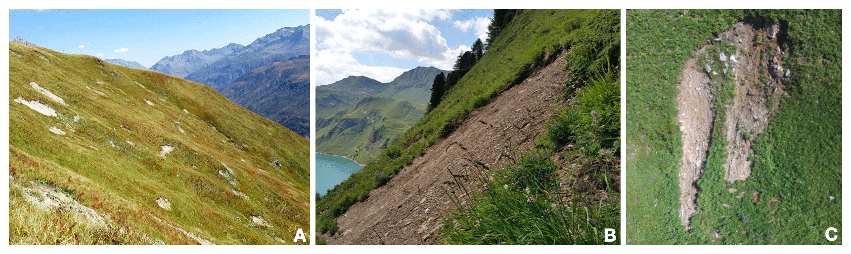
Figure 1 Images showing examples of shallow landslides. Shallow-landslide sites show displaced topsoil layers and have a distinct boundary to the vegetation. (a) Taken in the Urseren valley, showing a larger section of a south-east-facing slope area affected by many shallow landslides (light-coloured patches). (b) Taken in Val Piora, showing a close-up of a shallow landslide facing south. (c) Showing an image taken with a UAV in Val Piora with an approximate length of 10 m.

The aim of our study is to statistically evaluate shallow-landslide occurrence for 10 different sites (between 16 and 54 km²) across Switzerland. In the past, shallow-landslide susceptibility studies have mainly focused on one or two study sites while often testing multiple modelling techniques (Gómez and Kavzoglu, 2005; Meusburger and Alewell, 2009; Vorpahl et al., 2012; Tien Bui et al., 2016; Oh and Lee, 2017; Lee et al., 2020; Nhu et al., 2020b), except for Persichillo et al. (2017), who evaluated four sites in different catchments. For our shallow-landslide inventory we map the eroded sites on aerial images (0.25 m resolution) using a U-Net deep learning approach (Ronneberger et al., 2015). The U-Net tool was trained by Samarin et al. (2020) to identify and map the extent of soil erosion features on grassland. While this mapping tool is able to distinguish between different erosion processes and appearances (i.e. shallow landslides, livestock trails, sheet erosion and management effects; Samarin et al., 2020), here, we focus on shallow landslides as we aim to understand their causal factors and spatial patterns better. With the U-Net mapping tool, we can identify locations of shallow landslides in a very efficient and precise manner, increasing the possibilities for mapping but also future model validation of soil erosion studies (Samarin et al., 2020). The mapped shallow-landslide sites are subsequently evaluated with a statistical model to identify the most important explanatory variables and gain a better understanding of causal factors as well as regional differences. For this purpose we use the group lasso approach for logistic regressions (Tibshirani, 1996; Yuan and Lin, 2006; Meier et al., 2008). The group lasso can deal with continuous and categorical variables and is able to estimate coefficients of classes within a categorical variable. In addition to estimating coefficients, the lasso can do variable selection simultaneously (Sect. 2.2). The lasso tends to yield sparse and interpretable models, avoids overfitting, and is tolerant towards possible collinearity of variables (Dormann et al., 2013). Despite these advantages, the lasso has only been applied a small number of times for landslide susceptibility modelling (Camilo et al., 2017; Lombardo and Mai, 2018; Amato et al., 2019; Gao et al., 2020; Lombardo and Tanyas, 2021; Tanyaş et al., 2021). We evaluate the shallow landslides within each study site (10 models) and across all 10 study sites simultaneously (all-in-one model) and consider only grassland surfaces. Our aim is to identify explanatory variables that have local importance but also identify variables which may explain regional differences in shallow-landslide occurrence. The selected study sites are a combination of alpine (above 1500 $\mathrm{m}\mathrm{a}.\mathrm{s}.\mathrm{l}.$) and foothill regions (below 1500 $\mathrm{m}\mathrm{a}.\mathrm{s}.\mathrm{l}.$) as well as one site in the Jura Mountains (below 1500 $\mathrm{m}\mathrm{a}.\mathrm{s}.\mathrm{l}.$). The explanatory variables we use are the same for all sites and consist of a combination of classic landslide susceptibility variables (Budimir et al., 2015) as well as climate-related variables (Karger et al., 2017, 2018), which may aid in explaining regional differences in shallow-landslide occurrence (Sect. 3.2). To understand how well the selected variables and their coefficients perform, we evaluate the models on held-out test data. We determine receiver–operator characteristic (ROC) curves and the corresponding area under curve (AUC) as well as the Brier score, which is suitable for binary variables (presence or absence of shallow landslides) (Sect. 2.3).

2 Study sites

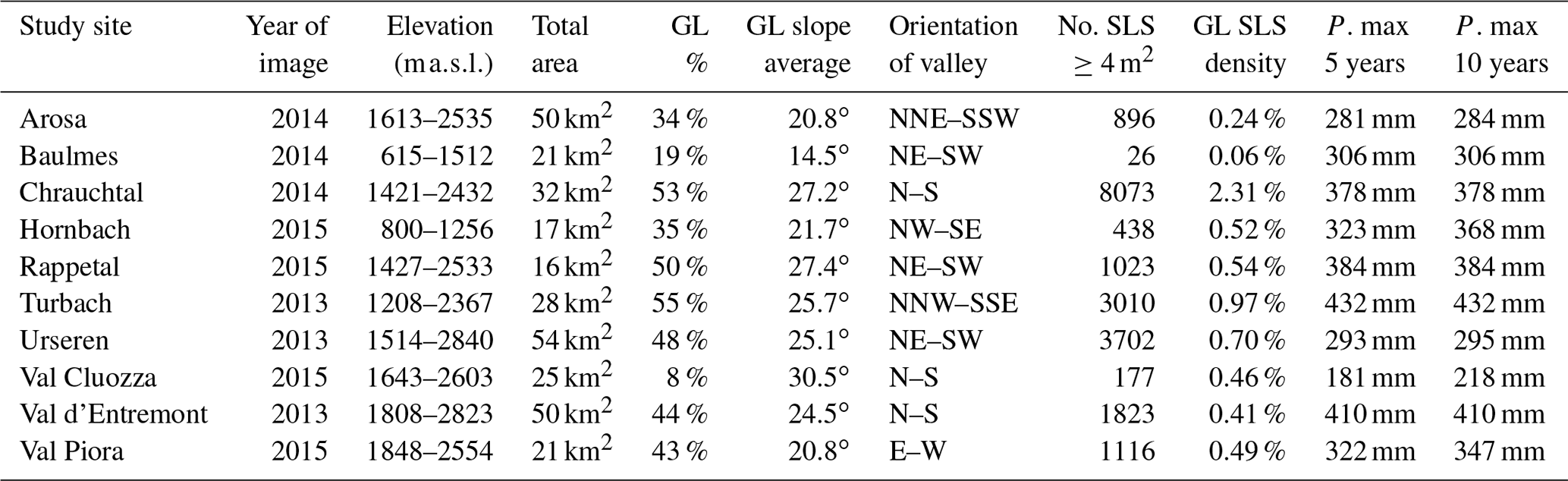
A total of 10 sites were selected to produce shallow-landslide inventories (mapping of shallow landslides) and perform subsequent statistical evaluations of explanatory variables. We only consider grassland areas, which were identified with the aid of the surface cover information of the product SwissTLM (Swisstopo, 2019). The sites were selected to represent different mountain and hill regions and different geological conditions, valley expositions and slope angles. Figure 2 shows the locations of all study sites within Switzerland, and Table 1 summarises important site information. Most permanent grassland surfaces in Swiss mountain regions are used for either grazing (pastures) or haying (meadows) (FSO, 2013; Stumpf et al., 2020). Of the 10 sites, 9 are located across the Swiss Alps, and 1 was selected in the Swiss Jura Mountains (Baulmes, below 1500 $\mathrm{m}\mathrm{a}.\mathrm{s}.\mathrm{l}.$). The sites located in the Swiss Alps represent a range of alpine (above 1500 $\mathrm{m}\mathrm{a}.\mathrm{s}.\mathrm{l}.$) regions as well as foothill regions (Hornbachtal, below 1500 $\mathrm{m}\mathrm{a}.\mathrm{s}.\mathrm{l}.$). Val Cluozza is located in the Swiss National Park and shows no signs of anthropogenic influences and also contains only a small amount of grassland area (8 %, the rest being mostly shrubs and rocks). For other sites in the Alps, grassland covers 34 %–55 % of the valley. The rest of the land cover consists of forest area, rock and debris area, or in some cases urban areas. The shallow-landslide densities (shallow-landslide-affected area in relation to total grassland surfaces) range from 0.06 % (Baulmes) to 2.31 % (Chrauchtal). Figure 2 shows the locations of all study sites within Switzerland, and Table 1 summarises important site information.

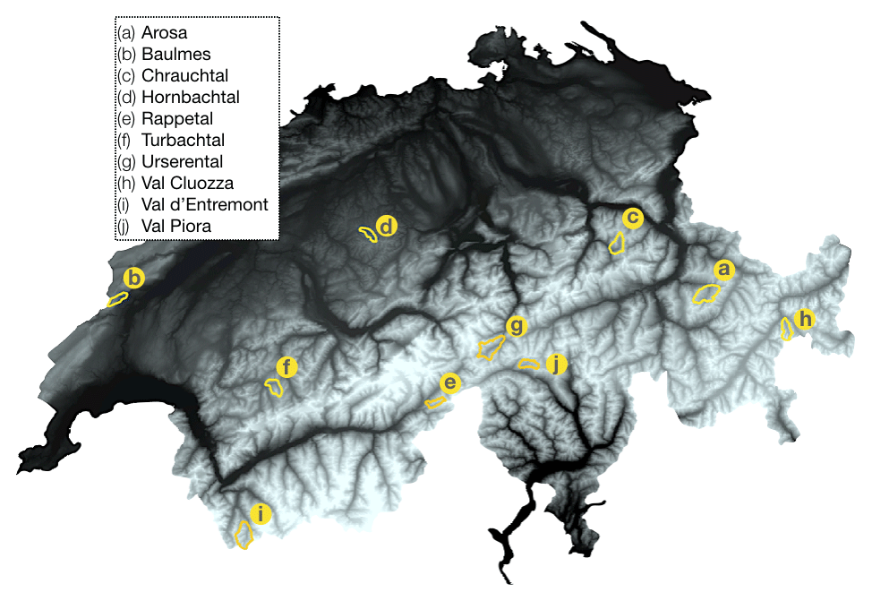
Figure 2 Map of Switzerland showing the 10 selected study sites (outlined in yellow). Colours of the map show lower elevations in dark and higher elevations in lighter colours. Digital terrain model obtained from © swisstopo.

Table 1 List of study sites and descriptive information: elevation range, total area of the study site, grassland area within study site in per cent, average slope of grassland area, orientation of the main valley axis, number of shallow landslides and shallow-landslide density in grassland areas. The max precipitation events (monthly values) of the previous 5 and 10 years are averaged over the study site. Note that both time spans might include the same events. GL: grassland; SLS: shallow landslides; P: precipitation.

2.1 Shallow-landslide inventory

To identify the locations of shallow landslides across the 10 study sites, we use a deep learning approach based on the U-Net architecture (Ronneberger et al., 2015). These mapped shallow landslides are then used for statistical evaluations of causal factors (Sect. 2.2). This fully convolutional neural network approach for semantic segmentation in images allows for objective and efficient mapping. The U-Net model was trained to identify and map erosion sites on aerial images (Swisstopo, 2010) with the aid of digital terrain model information (Swisstopo, 2014), as described in Samarin et al. (2020), and can be obtained from Samarin (2021). The U-Net model was trained on a small area of 9 km² and tested on an area of 17 km² in the Urseren Valley (Samarin et al., 2020). For this study we use the same U-Net model without further training to map the new study sites and focus only on the erosion class shallow landslides, as defined in the introduction. The mapping results were carefully examined for all study areas and corrected manually when necessary. The trained U-Net used in this study has an overall precision of 73 %, a recall of 84 % and an F1 score of 78 % (Samarin et al., 2020). We only consider shallow landslides of at least 4 m² located on grassland (see Fig. 4 for examples of mapping results and in Fig. S11 in the Supplement for an example of one fully mapped study site).

2.2 Logistic regression with group lasso

With the statistical evaluation of the shallow-landslide sites, we aim to understand possible causal factors. We evaluate the 10 study sites individually (evaluation within each site) as well as across all of the sites simultaneously (all-in-one model). The aim of this is to test whether the same causal factors are important on different spatial scales. For each of the 10 sites an equal number of shallow-landslide and non-landslide points constitute the binary response variable (no = 0, yes = 1) with a set of corresponding explanatory variables (see Sect. 3). Our aim is to use a method that generates sparse models that are easy to interpret and avoid overfitting. To achieve this, we use a logistic regression estimated with the least absolute shrinkage selection operator (lasso) (Tibshirani, 1996). The lasso regression performs variable selection and coefficient estimation simultaneously. This is obtained by applying a penalty term (II) to the log-likelihood function of the logistic regression (I) (Hastie et al., 2016):

$$\begin{array}{}\text{(1)}& \begin{array}{rl}& {\mathrm{\ell }}_{\mathit{\lambda }}\left(\mathit{\beta }\right)\\ & =x\underset{\text{I.}}{\underbrace{-\sum _{i=\mathrm{1}}^n\left(y_i{z}_{\mathit{\beta }}\left({\mathit{x}}_i\right)-\log \left(\mathrm{1}+e^{z_{\mathit{\beta }}\left({\mathit{x}}_{\mathit{i}}\right)}\right)\right)}}+\mathit{\lambda }\underset{\text{II.}}{\underbrace{\sum _{j=\mathrm{1}}^p|{\mathit{\beta }}_j}}|.\end{array}\end{array}$$

We consider the linear model $z_{\mathit{\beta }}\left(\mathit{x}\right)={\mathit{\beta }}_{\mathrm{0}}+{\sum }_{j=\mathrm{1}}^p{\mathit{\beta }}_j{x}_j$ on a data set of size n with p features, i.e. x_i∈ℝ^p, and binary response $y_i\in \mathit{\{}\mathrm{0},\mathrm{1}\mathit{\}}$. The penalty term is determined by the parameter λ, which is estimated by minimising the model error. The weight of λ determines how many variables are selected, and in turn, the model shrinks coefficients of variables that contribute to the error (Hastie et al., 2009, 2016). By shrinking the coefficients of unimportant variables to zero, they are removed from the model, and thereby variable selection is performed. To achieve the least complex model in terms of selected variables, we chose λ to be 1 standard error larger than the minimal mean square error (Hastie et al., 2009). As some of the explanatory variables are categorical (i.e. geology, aspect) we use the group lasso approach. All levels within a categorical variable (encoded as dummy variables) are treated as a group, and all coefficients within that group become zero (dismissed) or non-zero (selected) simultaneously (Yuan and Lin, 2006; Hastie et al., 2016). This leads to a new objective function with modified penalty term,

$$\begin{array}{ll}{\displaystyle }{\mathrm{\ell }}_{\mathit{\lambda }}\left(\mathit{\beta }\right)=& {\displaystyle }-\sum _{i=\mathrm{1}}^n\left(y_i{z}_{\mathit{\beta }}\left({\mathit{x}}_i\right)-\log \left(\mathrm{1}+e^{z_{\mathit{\beta }}\left({\mathit{x}}_{\mathit{i}}\right)}\right)\right)\\ \text{(2)}& {\displaystyle }& {\displaystyle }+\mathit{\lambda }\sum _{g=\mathrm{1}}^G{\mathit{\alpha }}_g\left|\right|{\mathit{\beta }}_g|{|}_{G_g},\end{array}$$

where α_g is a scaling factor depending on the number of parameters in β_g, and $\left|\right|\mathit{\eta }|{|}_K=({\mathit{\eta }}^{T}K\mathit{\eta }{)}^{\mathrm{1}/\mathrm{2}}$ is a norm depending on the group structure of the G different groups. For more details on the mathematical extension of the group lasso we refer to Meier et al. (2008). We implement the group lasso for logistic regression with the R package grpreg (Breheny and Huang, 2015). Due to the spatial relationship of geographic data sets, we divide the data into spatially separated blocks of 1 km², randomly numbered from 1 to 5 (Valavi et al., 2019) (see Fig. 3). These blocks are used for fivefold cross-validation of the model. Every block is held out once for testing, while the others are used for model training (e.g. while blocks labelled with 2, 3, 4 or 5 are used for training, blocks labelled with 1 are used for model testing). During each fold, coefficients are estimated for the explanatory variables. Note that the explanatory variables have been standardised to allow for easier comparisons between variables. The estimated values of the coefficients, therefore, give an indication of their relative importance to model the response variable (shallow-landslide and non-shallow-landslide points). With higher absolute values of an estimated coefficient, the influence of this explanatory variable is stronger. A linear transformation would be performed to ultimately get the coefficients for the variables on their original scale (Lombardo and Mai, 2018). The process of coefficient estimation is repeated 20 times (bootstrapping) with different randomly selected blocks, generating 100 estimates of coefficients for every site (20 fivefold cross-validations) (Goetz et al., 2015; Steger et al., 2016). We assess the model-selected coefficients by evaluating the range of the coefficient estimates (boxplots) as well as their inclusion rate (number of times selected by models) as the number of ideal variables can vary in each fold.

Figure 3 Spatial blocks for fivefold cross-validation shown with the example of Chrauchtal. Blocks have a size of 1 km². Blocks are assigned randomly and determined with the R package blockCV (Valavi et al., 2019).

2.3 Model evaluation

To evaluate the accuracy and the predictive ability of the logistic regression models, we use performance measures described in the following. All model performances are based on test set estimations (predictions evaluated on held-out test data blocks). The receiver–operator characteristic (ROC) curve is a continuous curve showing the relationship between the true positive rate (TPR) and false positive rate (FPR) for every probability threshold of the model predictions (Hosmer and Lemeshow, 2000). The accompanying area under curve (AUC) is the integrated area under the ROC curve and describes the model skill across all possible probability thresholds. Values of the AUC above 0.5 (equivalent to a random model) are better, while a score of 1 indicates a perfect model. Additionally, we compute confusion matrix performance scores for a fixed probability prediction threshold of 50 %. To summarise the accuracy of the models, we assess the magnitude of the error in the probability predictions using the Brier score (BS) (Eq. 3) (Brier, 1950; Wilks, 2006).

$$\begin{array}{}\text{(3)}& {\displaystyle }{\displaystyle }\text{BS}={\displaystyle \frac{\mathrm{1}}{N}}\sum _{t=\mathrm{1}}^N(f_t-o_t{)}^{\mathrm{2}},\end{array}$$

where N is the number of mapped shallow landslides, f_t represents the predicted probabilities for shallow-landslide occurrence (between 0 or 1), and o_t represents the observed (mapped) shallow landslides (either no = 0 or yes = 1). The Brier score (BS) is equivalent to the mean squared error yet is valid for binary observations. A BS of 0 indicates perfect model performance, while 1 is the worst possible score (prediction is opposite of observation). Probability predictions that are farther away from the observation are penalised more heavily. If the model predicts a 50 % chance of shallow landslide every time (random), a score of 0.25 is achieved for a balanced data set (Steyerberg et al., 2010; Raja et al., 2017). We re-estimate the BS with bootstrapping (500 repetitions, sampled with replacement) to achieve confidence intervals.

3 Data Sets

3.1 Shallow-landslide and non-landslide points

To perform the mapping of shallow-landslide sites with the U-Net model (Sect. 2.1), we require aerial (ortho-)images (SwissImage; Swisstopo, 2010) and a digital terrain model (DTM; SwissALTI; Swisstopo, 2014). The aerial images have a spatial resolution of 0.25 m and red, green and blue spectral bands. The aerial images for the study sites were collected during the years 2013 (Turbach, Urseren, Val d'Entremont), 2014 (Arosa, Baulmes, Chrauchtal) and 2015 (Hornbach, Rappetal, Val Cluozza, Val Piora). From the DTM, the derivatives slope, aspect and curvature (plan and profile) are required, which are calculated with ArcGIS (10.5). Additionally, we use a data set with land-cover information (SwissTLM, Swisstopo, 2019) to assure only sites with grassland are being mapped. For the mapped shallow landslides, we extract the centre points with ArcGIS of sites with a minimum size of 4 m². Non-landslide points were extracted randomly within the grassland area and with a minimum buffer distance to mapped shallow landslides of 5 m. This shallow-landslide data set contains an equal number of landslide and non-landslide points for each study site (Fig. 4) (Frattini et al., 2010; Petschko et al., 2014).

Figure 4 Example of mapped shallow landslides in the Turbach valley (purple). The centred points (yellow) represent shallow-landslide locations for the lasso model evaluation. Only sites with an area larger than 4 m² were used for the evaluation. Red points represent randomised non-landslide points. Aerial image (2013) obtained from © swisstopo.

3.2 Explanatory variables

The explanatory variables selected for the statistical evaluation of the shallow-landslide points are a combination of variables commonly found in landslide or shallow-landslide susceptibility studies (Budimir et al., 2015; Chen et al., 2017; Cignetti et al., 2019; Kavzoglu et al., 2014; Lee et al., 2020; Meusburger and Alewell, 2009; Persichillo et al., 2017; Nhu et al., 2020a, b) and climate-related variables that may explain differences between the sites (e.g. strong precipitation events) from the CHELSA data set (Karger et al., 2017, 2018). Variables related to land cover and vegetation are not considered as we filter our study sites to contain only grassland areas.

Table 2 Table containing the variables used for the logistic regression with information on the type of variable (continuous or categorical), spatial resolution and which data set the variable was originally based on.

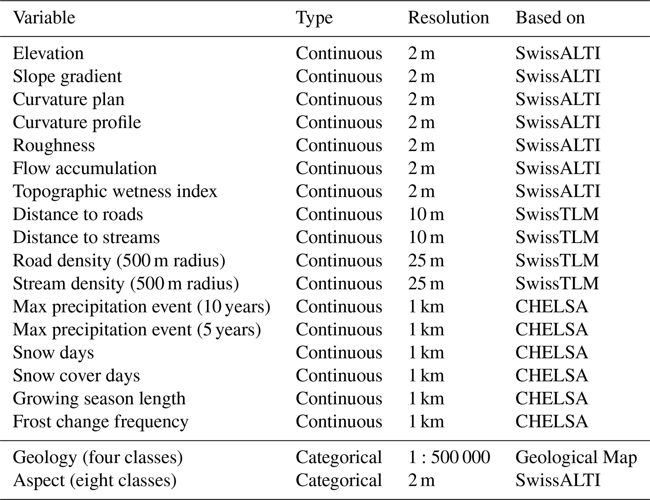
For every shallow-landslide and non-landslide point the variables listed in Table 2 were extracted. The same variables are used for evaluating all 10 sites as well as the all-in-one model. The continuous variables have been standardised to allow for comparing coefficients of variables. The categorical variables were converted to dummy variables (all classes of a categorical variable encoded as 0 or 1). Most variables can be derived from the DTM (elevation values, SwissALTI), which has a spatial resolution of 2 m. Slope (in degrees) describes the maximum change in elevation to neighbouring cells. Aspect is included as a categorical variable containing eight exposition sectors (north, north-east, east, south-east, south, south-west, west and north-west). For curvature we use plan and profile. Plan curvature describes the slope's concave (positive values) or convex (negative values) properties perpendicular to the direction of the maximum slope, while profile curvature indicates the same but parallel to the maximum slope. A value of zero indicates a flat surface. Plan curvature characterises the convergence and divergence of surface flow, and profile curvature describes the acceleration of the surface flow (Zevenbergen and C., 1987). Roughness expresses the difference between maximum and minimum elevation values between a cell and all of its neighbouring cells (Wilson et al., 2007). Higher roughness values indicate rougher terrain. Based on flow direction (direction of the steepest descent) we determine the flow accumulation, which describes the number of cells flowing into a cell. The topographic wetness index (TWI) gives indications of where water accumulates on slopes and is calculated with $\ln (\mathit{\alpha }/\tan \mathit{\beta })$, where α is the upslope area draining through a certain point per unit contour length (flow accumulation), and β is the slope (Beven and Kirkby, 1979). Distance to roads and road density are variables that are often included in landslide susceptibility studies as they represent constructional interference (Meusburger and Alewell, 2009; Nhu et al., 2020b). Distance to streams and stream density can give further information on rainfall drainage and runoff processes (Nhu et al., 2020b). These variables were calculated based on the SwissTLM data set (Swisstopo, 2019), containing information on road and stream locations using the distance and line density tool (search radius of 500 m; Meusburger and Alewell, 2009) of ArcGIS. In addition to these terrain-related variables, we use variables derived from the CHELSA data set, which contains monthly values on temperature and precipitation from which many environmental parameters are derived (Karger et al., 2017, 2018). We include the strongest precipitation events of the last 5 years and 10 years prior to the recording year of the aerial images, information on snow fall and cover, growing season length, and frost change frequency (5 year average of 2009–2013). While these variables have a comparatively low spatial resolution (30 arcsec, approx. 1 km), they may give a good indication of regional differences in shallow-landslide occurrence as they are representative of alpine processes often linked to the triggering of shallow landslides (Meusburger and Alewell, 2008; Wiegand and Geitner, 2010; Löbmann et al., 2020; Geitner et al., 2021). Specifics on the individual CHELSA variables used can be found in Karger and Zimmermann (2019). Since we analyse 10 different sites as well as all sites in one model, we select a simplified geological data set containing only the three main rock formation classes (igneous, metamorphic, sedimentary) and unconsolidated rocks. This reduces the number of classes in the categorical variable and increases the interpretability of the model, especially when comparing between sites.

4 Results and discussion

The lasso regression model selects the relevant explanatory variables and estimates their regression coefficients to predict the location of shallow landslides. The statistical evaluation was conducted for all 10 sites individually and for all sites combined into one large model (all-in-one model). The same explanatory variables were used for both approaches. Due to the 20 fivefold cross-validations and random re-samplings (bootstrapping), the coefficients are estimated 100 times. The estimated coefficients should be analysed in combination with the variable inclusion rate, which describes how many times the explanatory variable was selected by the lasso regression model (100 = selected every time) and gives an indication of the importance of the variable.

4.1 Individual-site models

The statistical evaluation of the study sites yields one model per site (10 models). We combine the results of all 10 sites in heat maps, showing the median estimated coefficients (Fig. 5) and their inclusion rate (Fig. 6).

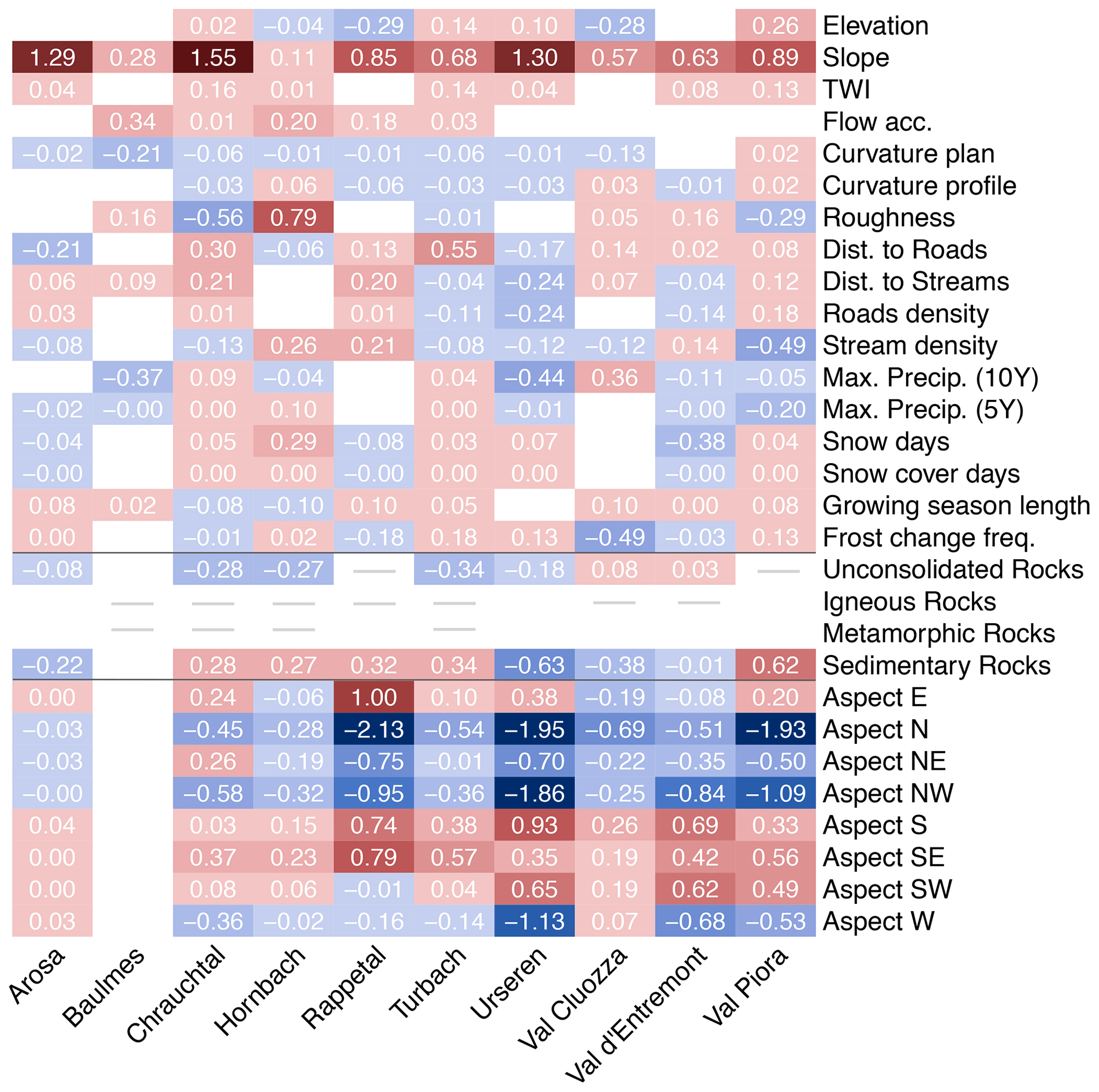
Figure 5 Heat map displaying estimates of coefficients (median of 100 estimates) for all 10 sites. Note that not all geological rock classes are present at all sites (grey line). White boxes are equivalent to coefficients of zero and were therefore never selected for the models.

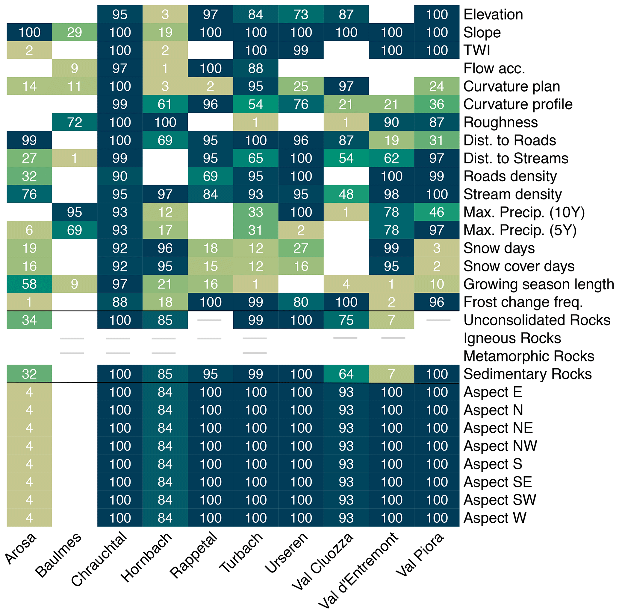
Figure 6 Heat map displaying the inclusion rate of variables for all 10 sites. The numbers indicate how often variables were selected for the models out of 100 estimates. Note that not all geological rock classes are present at all sites (grey line). Darker colours show variables selected more often. White boxes indicate which variables were never selected for the models.

Most sites select slope as the most important variable in terms of coefficient value as well as the inclusion rate. Only the sites Baulmes (29 %) and Hornbach (19 %) rarely select slope and shrink the value of the coefficient towards zero. These sites are both located outside of the Alpine region (Jura Mountains and the foothills of the Alps) and on average have gentler slopes (Baulmes 14^∘ and Hornbach 21^∘). Steeper slopes tend to be more susceptible to shallow landslides, which is in agreement with other studies that have found slope to be one of their top predictors (Budimir et al., 2015; Goetz et al., 2015; Tien Bui et al., 2016; Oh and Lee, 2017; Persichillo et al., 2017; Lombardo and Mai, 2018; Lee et al., 2020; Nhu et al., 2020a, b).

The aspect was selected most times (84 %–100 %) for all sites except for Arosa (4 %) and Baulmes (0 %) (Fig. 6). In Baulmes, this may relate to the fact that there are only 26 mapped shallow landslides available and that all grassland areas in the valley are located on the south-east-facing slope, which includes non-landslide points. The rest of this site is covered with forest, which was not considered for our evaluation. Arosa is located in a wide circular-shaped valley with no dominant slope expositions, and no typical aspect for shallow landslides is present. For the remaining eight sites, the sectors ranging from west to north-east are strong indicators of no shallow landslides occurring, while E–SW-facing slopes are favourable for shallow landslides (Persichillo et al., 2017; Lombardo and Mai, 2018). The coefficient size of the individual aspect sectors varies slightly from site to site, indicating that aspect may be more predictive in some areas (e.g. Urseren or Val Piora) than in others (e.g. Hornbach or Val Cluozza).

Other important variables which show a high inclusion rate amongst most sites yet often do not have a large impact concerning the coefficient values are roughness, TWI, distance to roads or streams, road or stream density, and frost change frequency. However, these variables were disregarded for some of the sites (low inclusion rates or even excluded completely). The coefficients' values may have a negative or positive correlation to shallow-landslide points (SLS points), depending on the sites and the local conditions. Geology is important for most sites, while sedimentary rocks and unconsolidated rocks are either present at the sites or selected for the model from all available classes. Unconsolidated rocks are negatively correlated in most cases. They can often be found near the valley bottom in proximity to streams and lakes, which tend to be located outside of shallow-landslide zones. Sedimentary rocks are positively correlated in most cases but can also show a negative correlation, depending on the site.

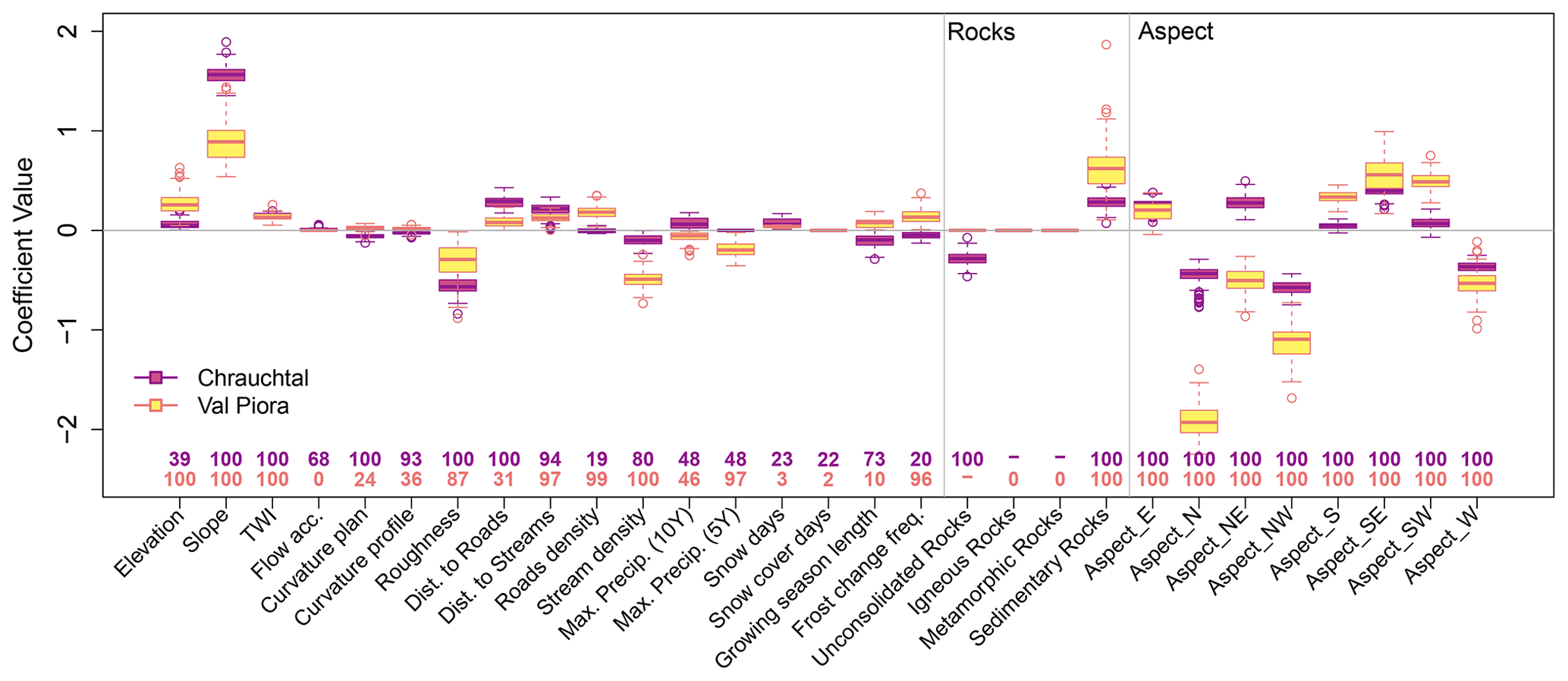
Figure 7 Boxplots (with whiskers and outliers) showing the coefficient range with 100 repetitions. Numbers above variable names indicate the number of times it was selected for the model. Boxes show the interquartile range (25th and 75th percentile), and the line indicates the median of the coefficients. Chrauchtal and Val Piora are selected from 10 study sites as examples.

Two sites (Chrauchtal and Val Piora) have been selected as examples to show detailed results of the models and how the selection of explanatory variables can differ between sites (Fig. 7). The boxplots of the estimated coefficients for all 10 sites can be found in the Supplement (Figs. S1–S10). Chrauchtal is located on the northern side of the Alps, while Val Piora is located on the southern side. They have opposing orientations of the main valley axis (N–S and E–W; see Table 1). Chrauchtal is the site with the highest shallow-landslide density (2.31 % with 8073 SLS points), which affects the very high inclusion rates for all explanatory variables (Fig. 6). This also affects the spread of the boxplots, which show small variability in the coefficient values (Fig. 7 in purple). With the high number of shallow landslides the variability in coefficients decreases, which means that the lasso regression estimates very similar coefficient values for all 100 repetitions. Val Piora has a lower landslide density (0.49 % with 1116 SLS points). Here, the spread of the boxplots shows a higher variability for the estimated coefficients (Fig. 7 in orange). Interquartile ranges are often much wider, and longer whiskers and outliers are more common than for the Chrauchtal site. For both sites, slope and aspect are very important variables in terms of coefficient size and inclusion rate. S–SW aspect sectors are susceptible to shallow landslides, while N–NW-facing slopes are unfavourable. Roughness is negatively correlated for both sites, meaning that rougher terrain is less favourable to shallow landslides. Variables with smaller coefficients may also be selected often by the lasso regression. However, these variables tend to have different effects depending on local conditions (e.g. distance to roads and road density, elevation, or TWI).

Table 3 Confusion matrix derivations using 0.5 for the prediction threshold. Perfect scores are accuracy = 1, bias = 1 (above 1 is overpredicted, while below 1 is underpredicted), true positive rate (TPR) = 1 and false positive rate (FPR) = 0. Site names are abbreviated as follows. A: Arosa; B: Baulmes; C: Chrauchtal; H: Hornbachtal; R: Rappetal; T: Turbachtal; U: Urserental; VC: Val Cluozza; VE: Val d'Entremont; VP: Val Piora.

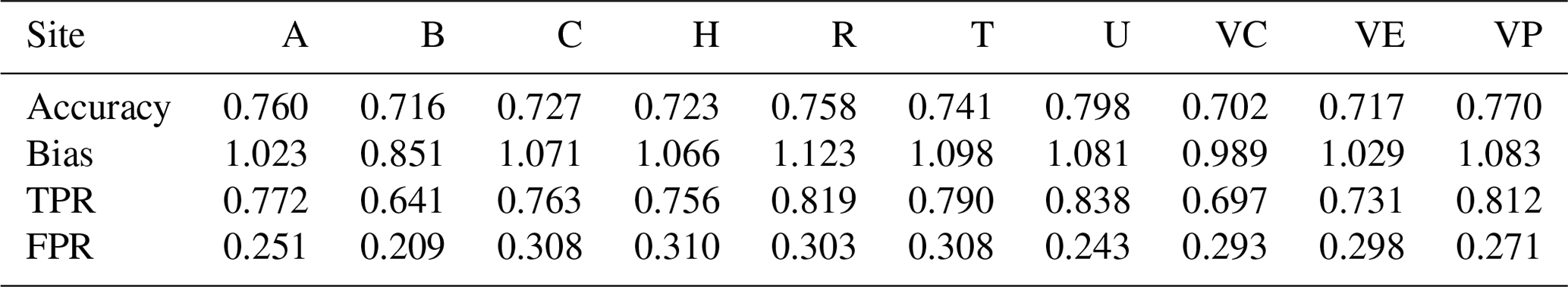
To assess the prediction skills of the individual-site models, we calculate the ROC curves and the corresponding AUC values (Sect. 2.3, Fig. 8). Curves closer to the top left corner of the plot show models with higher predictive skills (e.g. Urseren, AUC = 0.865), while curves closer to the diagonal line have lower predictive skill (e.g. Baulmes, AUC = 0.733). Confusion matrix scores summarised in Table 3 are based on a probability threshold of 0.5, which is the best threshold based on ROC curve evaluation (not shown). Brier scores describe the accuracy of the predictions, where values closer to zero indicate better model performance (Sect. 2.3, Fig. 9). The Urseren site has the best model accuracy (BS = 0.14), while Baulmes has the lowest score (BS = 0.21, located in the Jura Mountains with only 26 SLS points). The remaining eight models have BS values that range between 0.16 and 0.19, which is satisfactory. Models of sites with more SLS points perform better and have a smaller spread of the bootstrapped BS. Sites with fewer SLS points do not perform as well. One exception is the Chrauchtal site (BS = 0.18), which has 8074 SLS points yet does not perform as well as other sites with fewer points. For models with higher Brier scores the selected explanatory variables might not have been suitable enough to predict the location of shallow landslides, whereas for sites such as Urseren and Val Piora, the available explanatory variables are well suited to describe the mapped shallow landslides.

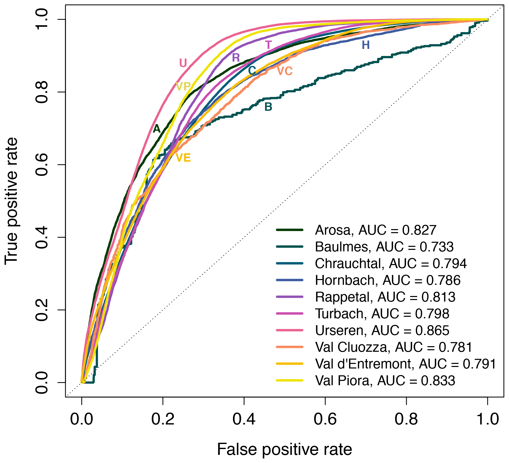
Figure 8 ROC performance measure of the models for all 10 sites. Plot displays ROC curves with corresponding AUC values.

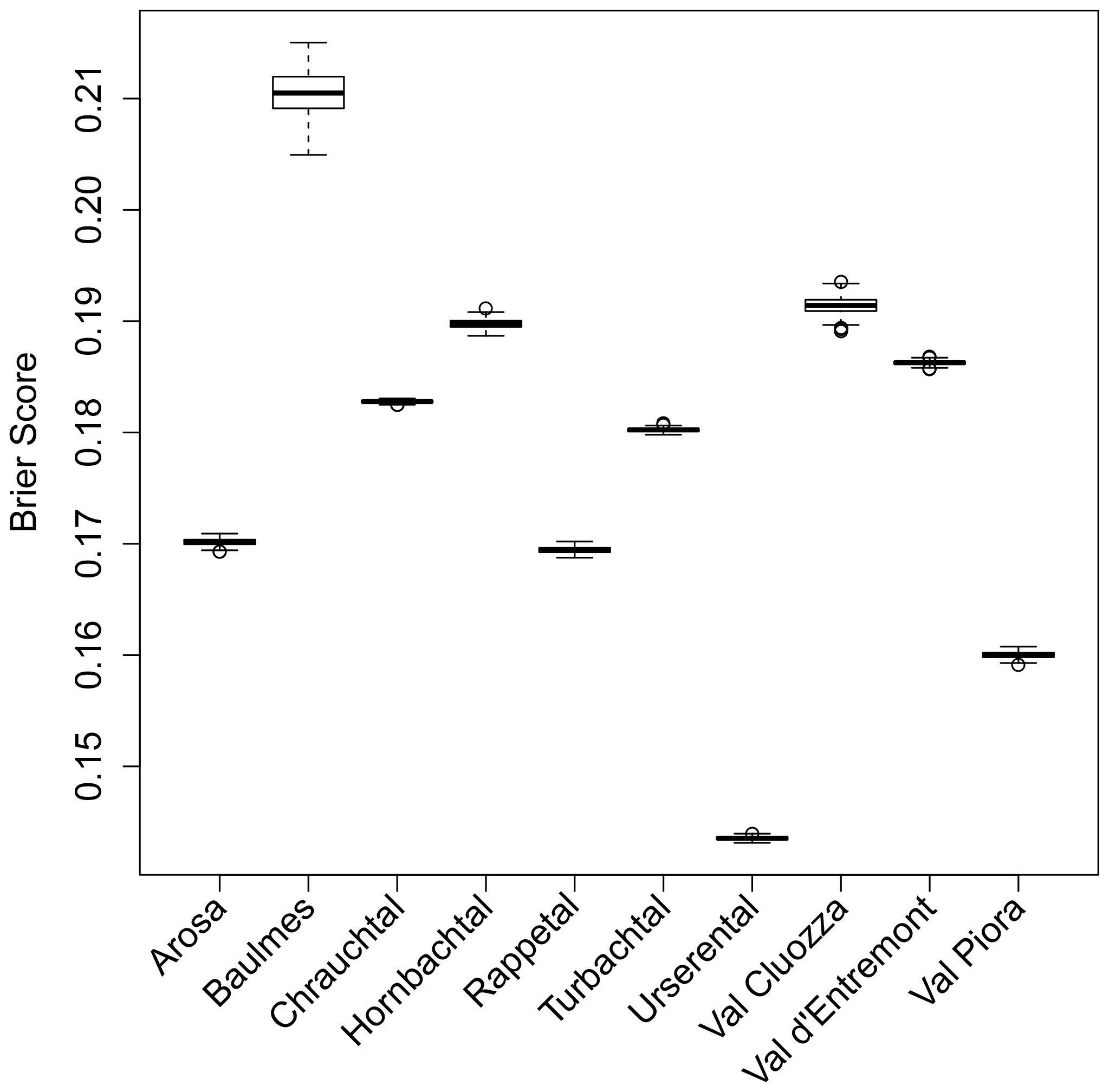
Figure 9 Performance measure expressed with the Brier score for the models for all 10 sites. Plot shows boxplots of Brier scores, where lower Brier scores are indicative of better model performance.

Generally, the number of shallow landslides available at a site does not necessarily affect the mean estimated value of coefficients, but the variability in the estimates is smaller, and the inclusion rates are higher for sites with more data points. Lower-performing models are for sites located either outside of the Alpine region (Baulmes, Hornbach) or in the Swiss National Park (Val Cluozza, only 8 % grassland in the valley) and have the lowest number of shallow landslides. This may be because different processes govern shallow landslides that are not covered by available variables. Alpine sites perform better, although performance measures can vary here too. Sites with better lasso regression model performance may be better explained with the available explanatory variables than other sites. Additionally, the better-performing models are for sites with an east–west orientation of the valley, independent of the number of shallow landslides. The latter implies that more slope surfaces are facing either south or north. South-facing slopes tend to be more susceptible to shallow landslides in the Alps as the exposition determines the amount of solar radiation (solar angle and duration). This, in turn, affects parameters such as evapotranspiration or soil moisture but also affects snow characteristics such as snow cover, snow movement or snowmelt, which have a strong influence on the occurrence of shallow landslides (Schauer, 1975; Moser and Hohensinn, 1983; Tasser et al., 2003; Meusburger et al., 2010; Wiegand and Geitner, 2013; Höller, 2014; Leitinger et al., 2018).

4.2 Performance of slope-only model

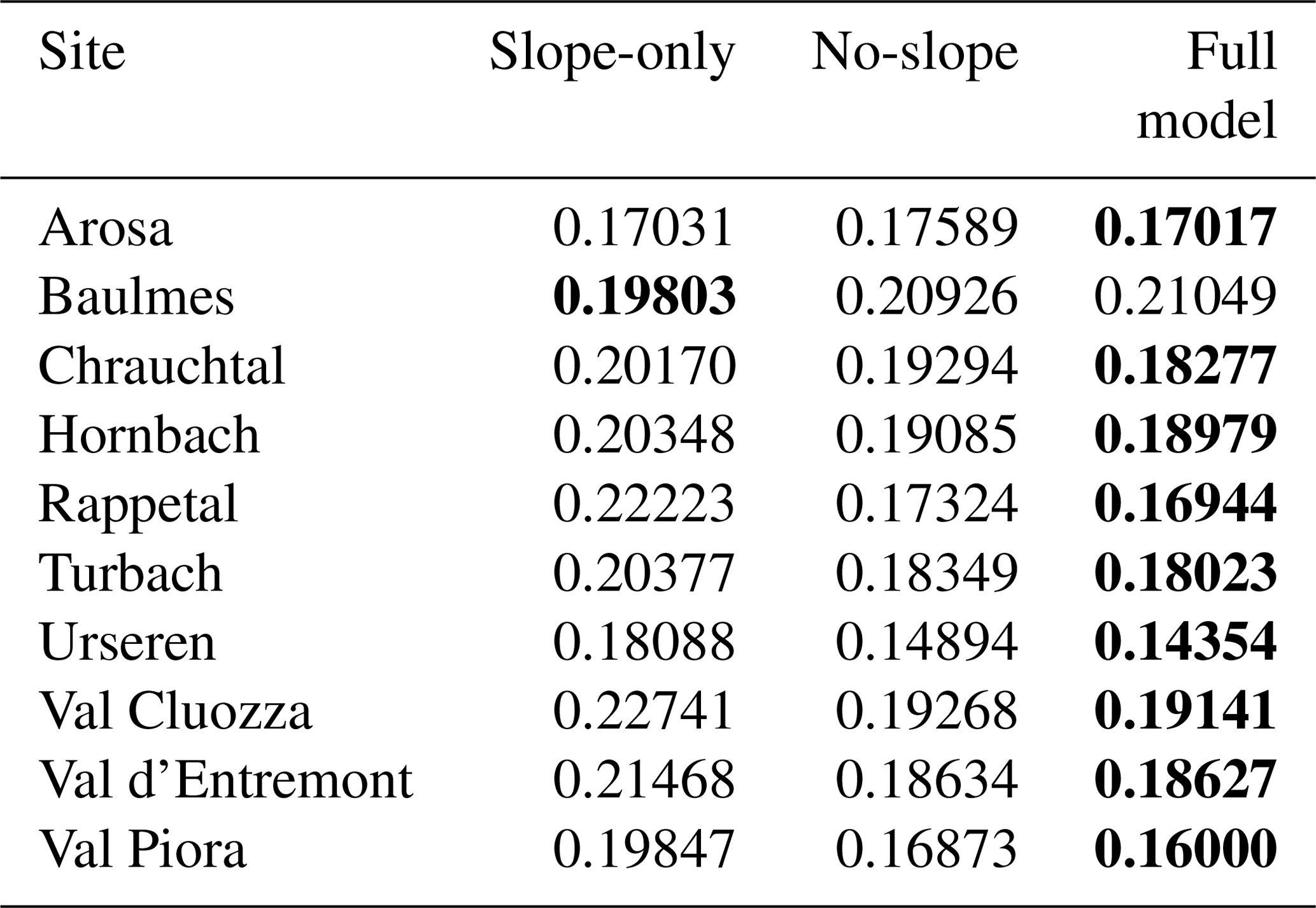
As the slope is always the most important predictor for shallow landslides in terms of coefficient size and model inclusion rates, a slope-only model was tested for all sites. The application of the slope-only model indicates how well slope predicts shallow landslides and how important additional explanatory variables can be. We therefore compare the results of slope-only models for all sites to the full-variable models based on their Brier scores (Table 4). Additionally, a no-slope model containing all predictors except for slope was included in the evaluation, demonstrating the additional importance of slope (full model) in comparison to all other predictors. Interestingly, for Baulmes with only 26 SLS points, the slope-only model performs slightly better than the full model. Arosa has only a slightly higher BS result for the full model compared to the slope-only model, which indicates that additional explanatory variables do not improve the model for Arosa very much. The importance of slope for Arosa can already be seen in Figs. 5 and 6. For all remaining sites, additional explanatory variables included in the model increase the model performance substantially. This is further supported by the higher BS results of the no-slope models. The differences between the slope-only, no-slope and the full models are statistically significant for all sites (paired t test with p values ≤0.05).

Table 4 Brier scores for the slope-only model compared with Brier scores of the no-slope and full models for all sites. The values displayed are median values of the bootstrapped Brier scores (500 repetitions). Lower scores are better (bold font) than higher scores.

4.3 Performance of all-in-one model

With the all-in-one model, we evaluate whether the same explanatory variables are important for cross-regional evaluations as for individual site evaluations. As all sites included in the all-in-one model have different numbers of SLS points, the sites with more points have a stronger influence on the model's outcome.

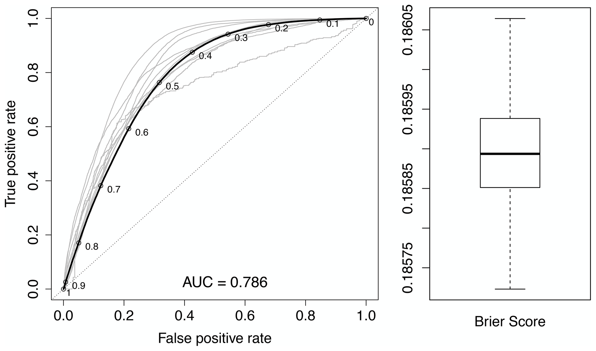
Figure 10 On the left-hand side, the ROC curve is displayed with the AUC value for the all-in-one model in black (including locations of probability thresholds) superimposed over the individual-site models in grey. On the right-hand side is the bootstrapped Brier score for the all-in-one model.

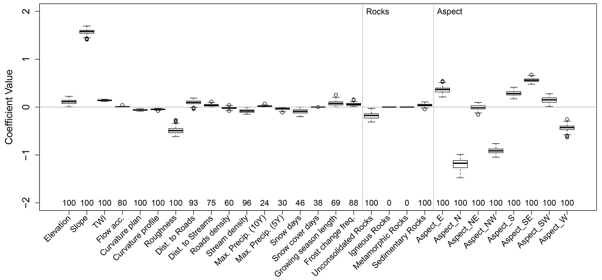
Figure 11 Boxplots showing the coefficient range with 100 repetitions. Numbers above variable names indicate the number of times it was selected for the model.

The all-in-one model places the ROC curve at roughly the centre of the individual-site models (Fig. 10), which is confirmed by the AUC value of 0.786. The same can be stated for the BS result (BS = 0.186). With a bias of 1.079, the all-in-one model only slightly over-forecasts shallow-landslide points, while the overall accuracy of 72.3 % is slightly below the average for the individual-site models (74.1 %). The true positive rate lies at 76.3 % and the false positive rate at 31.6 %, which is slightly higher than all individual-site models. Generally, the individual-site models perform better in most cases as local conditions are important for the overall accuracy of models. However, the variability in the estimated coefficients of the all-in-one model is relatively low (Fig. 11), indicating that the coefficients were estimated similarly when selected.

The most important variables are comparable to the individual-site models, with slope and roughness having the largest coefficients for continuous variables (Goetz et al., 2015). The categorical variables aspect and geology show similar behaviour to the individual-site models. The CHELSA climatology variables (max precipitation events, snow days and snow cover days, growing season length, and frost change frequency) were originally included with the idea that these might have a stronger impact when doing cross-regional evaluations such as this all-in-one model. From these variables, frost change frequency was selected the most (88 %). Frost change frequency describes the number of daily events for which the temperature encompasses zero (Karger and Zimmermann, 2019), yet the estimated coefficient is very small. This variable was tested as it may represent snow movement processes related to freezing–thawing cycles, yet it was too ambiguous. Other climate variables were rarely selected. The inclusion of climate variables may prove helpful when comparing different regions in a “bulk” perspective (e.g. average landslide density per site) but seemingly not when explaining locations of individual shallow landslides across different regions. Additionally, the comparatively low spatial resolution of the CHELSA data set (30 arcsec) may not be suitable for such detailed analysis, and the variables might not represent triggering landslide processes well enough.

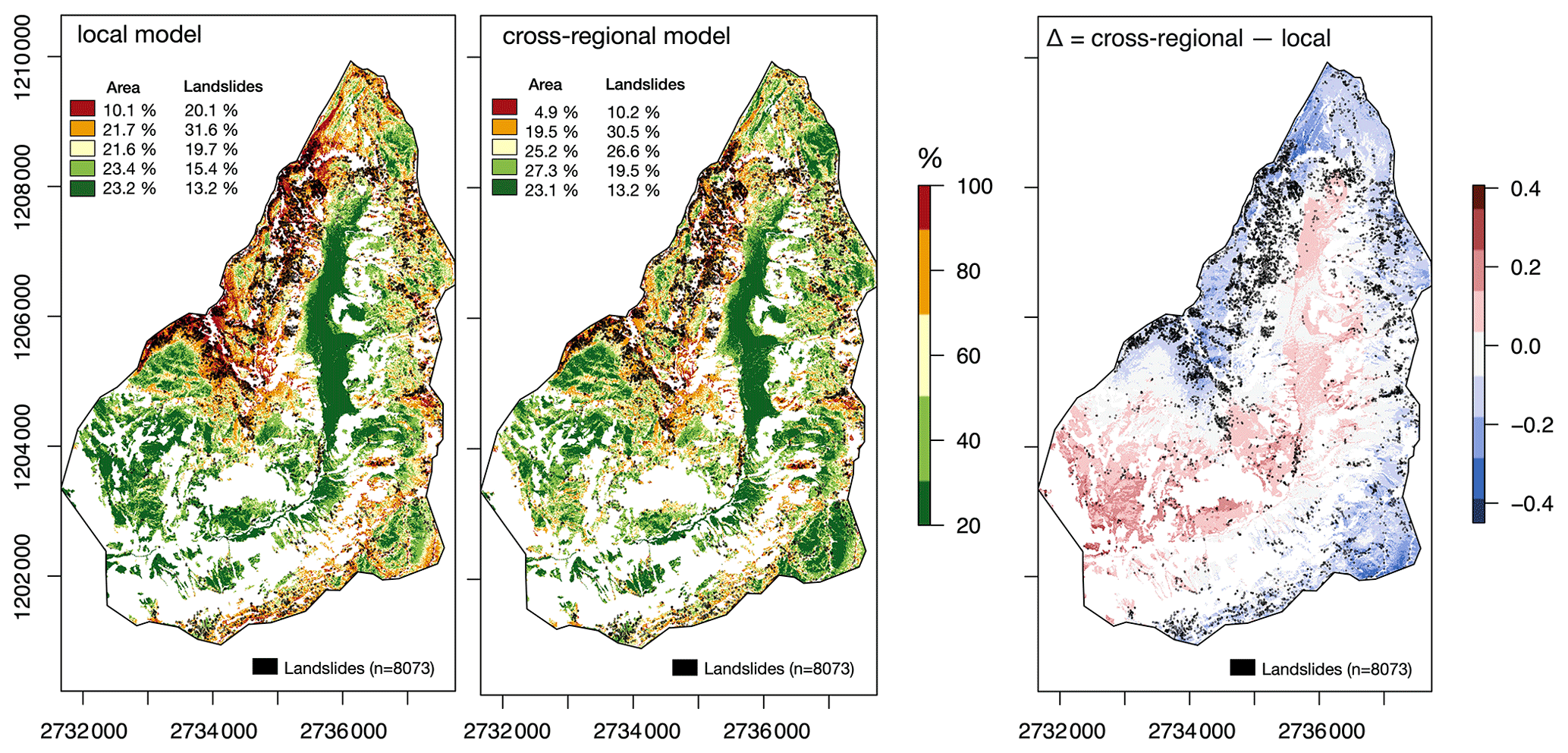
Figure 12 Susceptibility maps for the study site Chrauchtal based on the local model and the cross-regional all-in-one model. The susceptibility maps show the probability of shallow landslides occurring at a specific pixel on the map. The difference between the two applied models are shown on the right-hand side. White areas on the map are not grassland and are therefore not considered.

Additionally, shallow-landslide causes can be manifold, and singular triggering processes are difficult to assign, and the timing of the occurrence is often unknown. If possible, it would be useful to differentiate between triggering factors of shallow landslides based on visual appearance, as was suggested by Geitner et al. (2021). With the U-Net approach used to map the shallow-landslide sites on aerial images (0.25 m), it is impossible to distinguish between triggering factors (Samarin et al., 2020; Zweifel et al., 2019). With higher spatial resolutions of climate variables and a temporal component to the mapped shallow landslides, it may become possible to assign triggering processes with such evaluation techniques. Additional variables such as land-use information (e.g. grassland management) could be of great importance if available in appropriate spatial resolution and high-enough accuracy for all regions (Meusburger and Alewell, 2009; Budimir et al., 2015). While the explanatory variables for this study were chosen based on data availability, this is not an exclusive list of possible predictors. Many studies have worked towards identifying triggering factors in varying Alpine regions, such as the effects of land use, snow processes, precipitation events or vegetation cover (Newesely et al., 2000; Tasser et al., 2003; Rickli and Graf, 2009; Wiegand and Geitner, 2010, 2013; Meusburger and Alewell, 2008; Meusburger et al., 2013; Von Ruette et al., 2013; Höller, 2014; Ceaglio et al., 2017; Fromm et al., 2018; Geitner et al., 2021). Therefore, it is difficult to fully quantify all ongoing processes simultaneously in such a complex system as triggering factors are often interlaced (Zweifel et al., 2019). To ideally represent causal factors for statistical evaluations of shallow landslides, these important processes need to be represented with high spatial resolutions, and a temporal component needs to be included (Meusburger and Alewell, 2009).

4.3.1 Susceptibility map

The calculated coefficients of the logistic regression may be used for spatial predictions of shallow-landslide occurrence, yielding a susceptibility map of the region for the remaining grassland areas. These susceptibility maps are useful to identify areas that may likely be affected by shallow landslides in the future (Barbb, 1984). As an example we used the site Chrauchtal to apply the coefficients of both the local model and the cross-regional all-in-one model (Fig. 12). As the coefficients are estimated 500 times per model, we use the mean coefficient values for the prediction process. The results are very similar; however, to highlight the differences between the local and cross-regional all-in-one model, a map showing the differences between the two maps is shown, where red regions show slightly higher probabilities of shallow landslides in the cross-regional all-in-one model, and blue areas show slightly higher probabilities in the local model. The blue areas mainly cover areas at higher elevations, whereas the red areas are located at lower elevations but are facing south. Working with cross-regional models allows the general pattern to be caught; however, local hotspots might be missed.

5 Conclusions

In this study we located shallow landslides across 10 study sites spread across Switzerland. We use the term shallow landslides to describe the erosion sites, which classifies the erosion feature without implications for the triggering event. Using the lasso regression model, we identified the most important explanatory variables for these shallow landslides located on grassland slopes. Due to the different local conditions of the varying sites, different explanatory variables were identified as important. Slope and aspect are among the most important variables. Shallow landslides of sites with an east–west orientation of the valley axis as well as alpine sites were better explained by the available explanatory variables (Urseren, Val Piora, Rappetal and Arosa). This means that exposition-related processes in mountainous regions are essential for understanding regional patterns (e.g. snowmelt, snow movement). For the remaining sites, the available selection of explanatory variables was not as well suited, and therefore important processes could be missed. Sites outside of the main Alpine region (Baulmes and Hornbach) or located in the Swiss National Park (Val Cluozza) have a small number of SLS points, which were not well explained by the available variables. Performance scores for individual-site models range between BS = 0.144, AUC = 0.865 (Urseren) and BS = 0.210, AUC = 0.733 (Baulmes). Although we find that slope was the most important variable, predictions using only slope yield lower accuracies, indicting that additional variables are important to explain local shallow-landslide occurrence. An all-in-one model evaluating all 10 sites simultaneously found comparable results to the individual-site models (i.e. slope and aspect), with performance values of BS = 0.186 and AUC = 0.786. Additionally, this model showed a relatively strong negative correlation for roughness, indicating that smooth grassland surfaces are more susceptible to shallow landslides. The decisive causal factors identified are generally related to static variables (e.g. geomorphological, geological), while the available climate-related data sets have proven to be less informative on both local and cross-regional scales. Nevertheless, data sets representing triggering shallow-landslide conditions and processes in appropriate spatial resolutions would likely improve model performance. Studies focusing on understanding small-scale processes are therefore of great importance, and with data availability shifting towards open access and higher spatial resolutions as well as large spatial coverage, such statistical evaluations may improve in the future.