Long-term magnetic anomalies and their possible relationship to the latest greater Chilean earthquakes in the context of the seismo-electromagnetic theory

Several magnetic measurements and theoretical developments from different research groups have shown certain relationships with worldwide geological processes. Secular variation in geomagnetic cutoff rigidity, magnetic frequencies, or magnetic anomalies have been linked with spatial properties of active convergent tectonic margins or earthquake occurrences during recent years. These include the rise in similar fundamental frequencies in the range of microhertz before the Maule 2010, Tōhoku 2011, and Sumatra–Andaman 2004 earthquakes and the dramatic rise in the cumulative number of magnetic anomalous peaks before several earthquakes such as Nepal 2015 and Mexico (Puebla) 2017. Currently, all of these measurements have been physically explained by the microcrack generation due to uniaxial stress change in rock experiments. The basic physics of these experiments have been used to describe the lithospheric behavior in the context of the seismo-electromagnetic theory. Due to the dramatic increase in experimental evidence, physical mechanisms, and the theoretical framework, this paper analyzes vertical magnetic behavior close to the three latest main earthquakes in Chile: Maule 2010 (M_w 8.8), Iquique 2014 (M_w 8.2), and Illapel 2015 (M_w 8.3). The fast Fourier transform (FFT), wavelet transform, and daily cumulative number of anomalies methods were used during quiet space weather time during 1 year before and after each earthquake in order to filter space influence. The FFT method confirms the rise in the power spectral density in the millihertz range 1 month before each earthquake, which decreases to lower values some months after earthquake occurrence. The cumulative anomaly method exhibited an increase prior to each Chilean earthquake (50–90 d prior to earthquakes) similar to those found for Nepal 2015 and Mexico 2017. The wavelet analyses also show similar properties to FFT analysis. However, the lack of physics-based constraints in the wavelet analysis does not allow conclusions that are as strong as those made by FFT and cumulative methods. By using these results and previous research, it could be stated that these magnetic features could give seismic information about impending events. Additionally, these results could be related to the lithosphere–atmosphere–ionosphere coupling (LAIC effect) and the growth of microcracks and electrification in rocks described by the seismo-electromagnetic theory.

1 Introduction

As earthquakes are geological events that might cause great destruction, studies about their preparation stage and generation mechanism are a matter of concern. That is why scientific studies offering new information, evidence, or insights about different physical mechanisms or activation insights gained during the seismic cycle improve our understanding of earthquake occurrences. Currently, one of the most controversial physical mechanisms that is being studied is the lithospheric electromagnetic variations as earthquakes' precursory signals. Nevertheless, the study of magnetic and geological relationships is not something new. For example, the decadal variations in the geomagnetic field have been associated with an irregular flow of the outer core (Prutkin, 2008). Thus, the secular variation in the magnetic field can be interpreted as the response of the movement of the fluid outer core interacting with the topography of the lower mantle. Then, as that topography in the core–mantle boundary corresponds to a projection of the topography of the Earth's surface (Soldati et al., 2012), it was not surprising that Cordaro et al. (2018) and Cordaro et al. (2019) found significant variations in geomagnetic cutoff rigidity R_c at relevant geological places in the Chilean margin.

Regarding earthquakes, many attempts to determine the location, date, and magnitude of seismic movements have been made in the past (e.g., Jordan et al., 2011), but these historical efforts have failed to conclude that it is possible to use seismological data as a predictive tool (Geller, 1997). Besides, less classical methods (e.g., electromagnetic methods) have been used for some decades. First attempts to address this topic can be found in the work of Varotsos–Alexopoulos–Nomicos (VAN) (see Varotsos et al., 1984, and the references therein). Techniques for seismic–electrical signals associated with the VAN method have been considerably improved and applied in several contexts (see Varotsos et al., 2019; Christopoulos et al., 2020, and the references therein). Also, some debates about this method can be found in the work of Hough (2010). Recently, electromagnetic methods have become more popular with relevant and conclusive evidence. Specifically, it is because a physical mechanism, based on the Zener–Stroh mechanism, links microcracks to magnetic anomalies and because a fault's friction is currently available (e.g., Stroh, 1955; Slifkin, 1993; Venegas-Aravena et al., 2019, 2020) that wide frameworks are being studied (holistic interaction between the lithosphere, ionosphere, and atmosphere, e.g., De Santis et al., 2019a; Yu et al., 2021). Moreover, different electromagnetic theories related to earthquakes have been implemented. For example, De Santis et al. (2017, 2019b) have shown the method of magnetic anomalies in which long-term magnetic data from different satellites (ionosphere level) are considered during quiet or non-disturbed periods in terms of the space weather. After removing a known magnetospheric process from data such as daily variation, the remaining magnetic perturbation or anomaly could be considered of lithospherical origin. This method allowed the authors to study magnetic measurements mostly free of external perturbation prior to and after 16 worldwide earthquakes of magnitude greater than approximately M_w 6.5. When satellites covered areas close to each earthquake's location, they found an increase in the number of magnetic anomalies prior to (1–3 months before) the occurrence of these earthquakes and a decrease after each earthquake (De Santis et al., 2017; Marchetti and Akhoondzadeh, 2018; Marchetti et al., 2019a, b; De Santis et al., 2019b).

Other methodologies also support certain statistical correlations to the earthquake's preparation phase. For instance, the rise in magnetic signals characterized by a wide range of ultra-low frequencies (5–100 mHz and 5.68–3.51 µHz) or the ionospheric disturbances before several earthquakes have been widely and intensively reported in the last couple of decades (Hayakawa and Molchanov, 2002; Pulinets and Boyarchuk, 2004; Varotsos, 2005; Balasis and Mandea, 2007; Foppiano et al., 2008; Molchanov and Hayakawa, 2008; Liu, 2009; Hayakawa et al., 2015; Contoyiannis et al., 2016; Potirakis et al., 2016; Villalobos et al., 2016; De Santis et al., 2017; Oikonomou et al., 2017; Cordaro et al., 2018; Marchetti and Akhoondzadeh, 2018; Potirakis et al., 2018; Ippolito, et al., 2020; Varotsos et al., 2019; Florios, et al., 2020; Pulinets et al., 2021; among others).

The magnetic phenomena rise not only during the decadal or preparation state but also during the fast coseismic stage. For example, small magnetic variations (∼ 0.8 nT) at ∼ 100 km were measured during the Tōhoku 2011 M_w 9.0 earthquake (Utada et al., 2011). Similar findings were shown by Johnston et al. (2006) during the Parkfield 2004 M_w 6.0 earthquake (∼ 0.3 nT) at ∼ 2.5 km. In addition, peaks of ∼ 0.9 nT were measured at ∼ 7 km during the Loma Prieta 1989 M_w 7.1 earthquake (Fenoglio et al., 1995; Karakeliana et al., 2002). The abovementioned reports have shown strong evidence of the presence of magnetic signals during the seismic preparation stage and during the rupture process itself. Up to this date, there have been several experiments and theoretical models that identify and explain the physical mechanism of different magnetic variations related to geological properties (e.g., Freund, 2010; Scoville et al., 2015; Yamanaka et al., 2016; Venegas-Aravena et al., 2019; Vogel et al., 2020; Yu et al., 2021). According to experiments, the rise in electrical current flux within rocks is due to the movement of imperfections and the sudden growth of microcracks when rock samples are being uniaxially stressed in the semi-brittle regime (Anastasiadis et al., 2004; Stavrakas et al., 2004; Ma et al., 2011; Cartwright-Taylor et al., 2014; among others). The applied external stress generates the internal collapse of rock, which implies the fast growth of microcracks and an increase in electrical currents that flow throughout the crack immediately before the failure of rock samples (e.g., Triantis et al., 2008; Pasiou and Triantis, 2017; Stavrakas et al., 2019). These currents created by this mechanism are known as pressure-stimulated currents (PSCs), and their rise occurs mainly when the rock samples abandon linearity (see Triantis et al., 2020, and references therein for further details). This pre-failure indicator has been used as the experimental base for theoretical descriptions of impending earthquakes at a lithospheric scale (Tzanis and Vallianatos, 2002; Vallianatos and Tzanis, 2003; Venegas-Aravena et al., 2019, 2020). This seismo-electromagnetic theory has explained the frequency range, the cumulative number of anomalies, the coseismic signals, friction states at fault, and the b-value time evolution by considering fast stress changes in the fault surrounding area. This area of fast stress changes was theorized by Dobrovolsky et al. (1979), and it can cover thousands of kilometers. Similarly, Venegas-Aravena et al. (2019) also found that the growth of microcracks and magnetic signals is caused by these stress conditions within this large area. Recently, large areas of fast stress and strain changes, which surround the impending earthquakes, have also been confirmed by GPS analysis (Bedford et al., 2020).

Despite the abovementioned evidence, there are still no reports of cumulative anomalies in one the most active margins: the Chilean margin (e.g., Vigny et al., 2011; Pedrera et al., 2014; Carvajal et al., 2017; Zhang et al., 2017; Abad et al., 2020; Satake et al., 2020). In Fig. 1 one can observe the strong historical earthquakes across the Chilean margin. Their occurrence is why this work presents a wide study of magnetic signals which include spectral (Fourier and wavelet analysis), cumulative, and space weather analysis 1 year before and after the three latest main megathrust earthquakes in Chile: Maule 2010 (M_w 8.8), Iquique 2014 (M_w 8.2), and Illapel 2015 (M_w 8.3). The space weather and general magnetic conditions are found in Sect. 2. The main magnetic and frequency analysis is defined and performed in Sect. 3. The relation between results and the physical mechanism from the seismo-electromagnetic theory is in Sect. 4. Finally, discussions and conclusions are in Sect. 5.

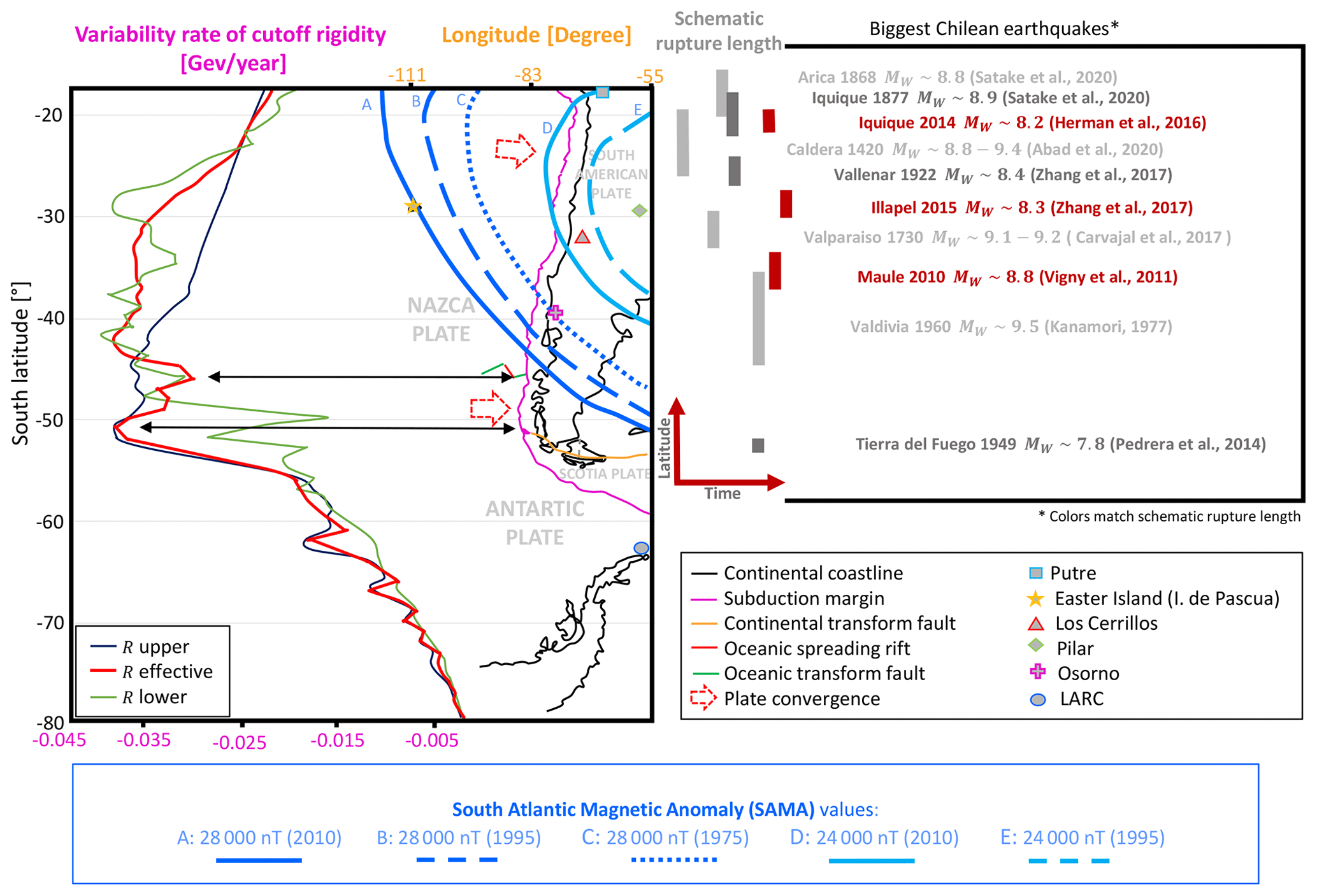
Figure 1 Left side: latitudinal effect of the geomagnetic cutoff rigidity projected over the Chilean convergent margin close to the 70^∘ W meridian. The solid pink lines indicate the edges of tectonic plates. The Nazca Plate is from 18^∘ N to 45^∘ S in latitude. The South American continent is on the South American Plate. The Antarctic Plate is from 45 to 79^∘ S. The black lines indicate the coastline. In blue are the iso-values of magnetic intensity due to SAMA proximity. The symbols indicate the stations' locations. Right: history of Chilean earthquakes.

2 Data processing consideration regarding the space weather and magnetic conditions

In order to perform a clear interpretation of the results, any methods and data processing must answer the classic questions: (1) what is actually being measured? (2) Where do the disturbances come from? (3) How should the disturbing data be removed? Here, the proper way to answer the abovementioned questions is by recognition of the physical process that generate external disturbances in measurements. Then, the standard index convention that identifies disturbed times and statistical analysis are used. This led us to implement four filters before working. These filters are as follows:

1. Disturbance storm time (Dst) filter. This filter eliminates periods of high solar magnetic activity. That is, the data within these periods are useless since the terrestrial cannot be distinguished from the solar.

2. Daytime filter (or quiet time). This filter eliminates daytime data as they reflect the interaction of the solar wind with the magnetosphere.

3. Stochastic filter. Moving averages eliminate the low-frequency variations associated with the usual flow of the ionosphere. Experiments and theory show that electrification of rocks prior to failure occurs mainly in the millihertz range (e.g., Triantis et al., 2012). Thus, moving averages filter the lower frequencies by using residuals methods to contain error propagation, that is, the difference between the signal and its smoothed signal.

4. Recurrence filter. This filter controls the failure of the other three filters, specifically, by using the definition of anomalous residuals which implies that any magnetic anomaly must be uncommon. Thus, the probability of finding an anomalous residual within a given period should tend to zero. In other words, few anomalies should be measured in the period. This indicates that if the number of detected anomalies dramatically increases, they are more common, and thus, not all of them can be considered anomalous. This contradiction could arise in two scenarios: (a) if a large number of anomalies occur during the entire period, the threshold should increase. (b) If a large number of anomalies occurs during a short period of time, let us say during 1 single day out of several months or years, then filters 1, 2, and 3 were insufficient to filter that specific day which implies that day cannot be considered.

Finally, the resulting filtered variations are potentially generated in the lithosphere, not in the space or ionospheric environment. It is important to note that the remaining data are almost unchanged since the analysis studies the applicable periods. With this added to records of several years, we eliminate some of the most significant concerns of the scientific community: the origin of disturbances, propagation of errors, and false positives. After this process, spectrograms or other methods can be used. That is, it requires very sophisticated preparation to discern and identify problematic disturbances in the records. This sophisticated filter process will be detailed in the following sections.

2.1 External magnetic disturbances

Before going into the study of the magnetic field and its temporal variations, it should be remembered that the rate of change in the magnetic field is influenced by the rate of variation in the spatial particle count. These are different cases of irregular and regular phenomena of the nearby space climate. Regular magnetic variation creates periodic fluctuations in the interplanetary magnetic field in a wide range of periods, from few-day periods up to seasonal variations (Moldwin, 2008; Blagoveshchensky et al., 2018; Yeeram, 2019). Irregular variations occur when sudden increases in incoming solar particles are recorded across the geomagnetic field. This particle disturbance induces a 10 % to 20 % decrease in magnetic field intensity because of the change in pressure that extraterrestrial particles exert on the magnetosphere, an effect that can last from a couple of hours to several days (Russel et al., 1999). One explication for the abovementioned effect comes from those particles that follow the magnetic field lines, in the turbulent magnetic reconnection that is present in the diurnal variation and the regular variations (Priest and Forbes, 2000; Kulsrud, 2004; Cordaro et al., 2016; Lazarian et al., 2020). Other minor irregular magnetic fields such as auroral events and electric current in the ionosphere are not considered for this paper (see Diego et al., 2005, for detailed description of these phenomena).

Some indices are used in order to measure the space disturbances and their manifestation in the geomagnetic field. For example, the Kp index measures the influence of geomagnetic storms in the horizontal magnetic field (Dieminger et al., 1996), while the Dst index is interpreted as a measure of the magnetospheric ring-current strength which is proportional to the particle's kinetic energy (e.g., Silva et al., 2017). Usually, the Dst index can increase by dozens or hundreds of nanoteslas during magnetic storms (Kp), which is why it is important to incorporate these indices to create reliable magnetic models.

2.2 Secular variation in the Chilean convergent margin

The magnetic response to these disturbances requires a reference model that allows the discrimination of Earth's magnetic features from disturbances that spread throughout interplanetary magnetic fields. One of those features corresponds to the magnetic shielding against incoming turbulent particles which is known as geomagnetic cutoff rigidity R_c (Pomerantz, 1971). The rigidity R_c is defined as the product of the force of the magnetic field and the curvature radius of the incident particle r_g, and it can be estimated globally by using the Tsyganenko magnetic field model (for details see Smart et al., 2000; Smart and Shea, 2001; Tsyganenko, 2002a, b). The R_c variations describe geomagnetic secular variations which could be related to geological features in the Chilean margin (Pomerantz, 1971; Shea and Smart, 2001; Smart and Shea, 2005; Herbst et al., 2013; Cordaro et al., 2018, 2019). For example, regarding the latitudinal effect (Pomerantz, 1971), Cordaro et al. (2019) found that the highest variation rate of effective R_c values were obtained at 46.5^∘ S, 76^∘ W and at 52^∘ S, 76.5^∘ W (Fig. 1). The first one is in the Taitao Peninsula, Chile, which corresponds to the triple junction point of three tectonic plates: Nazca, South American, and Antarctic. The second one is close to Puerto Natales in the Strait of Magellan area, also a triple junction point of three tectonic plates: South American, Antarctic, and Scotia (Fig. 1). There are other geological and geomagnetic links such as the flat slab in the Chilean convergent margin (Cordaro et al., 2018, 2019). However, these results are not surprising because changes in R_c represent secular variations that represent magnetic secular variations created at the outer core (Bloxham et al., 2002; McFadden and Merrill, 2007; Sarson, 2007; Finlay, 2007; Herbst et al., 2013). Specifically, 3D models of core mantle boundary (CMB) topology based on the velocities of seismic waves (Simmons et al., 2010) show the existence of positive topography in upthrust regions and negative topography in subduction zones (Yoshida, 2008; Lassak et al., 2010; Soldati et al., 2012). Let us remark that the intensity of the geomagnetic field within the outer core is estimated to be of the order of 2–4 mT (rms) (Olson et al., 1999; Olson, 2015), while at the Earth's surface it varies between 20 000 and 60 000 nT.

The most relevant magnetic feature in the Chilean sector is the low magnetic intensity values that correspond to the influence of the South Atlantic Magnetic Anomaly (SAMA) (e.g., Cordaro et al., 2016). Recently, Tarduno et al. (2015) argued that SAMA is being created by a topography structure in the CMB beneath southern Africa. Not only is SAMA linked with global magnetic features such as a geomagnetic dipole moment (e.g., Heirtzler, 2002; Gubbins et al., 2006), it also corresponds to the closer area between the Earth's surface and radiation belt. This proximity allows more charged particles and more disturbances in the magnetic field near the Chilean margin (e.g., Kivelson and Russell, 1995). That is why a proper magnetic response to external disturbances is required before and after earthquake occurrences.

2.3 Magnetic perturbation during seismic events of 27 February 2010 in Maule, 1 April 2014 in Iquique, and 16 September 2015 in Illapel

The manifestation of a space climate in the geomagnetic field during the periods concerned is defined by the Kp magnetic activity index as shown in Fig. 2 for the months prior to the three earthquakes: Maule 2010 (12 December 2009 to 15 March 2010), Iquique 2014 (1 January 2014 to 15 April 2014), and Illapel 2015 (1 July 2015 to 30 September 2015). For Maule 2010 the magnetic activity reached a Kp index equal to or greater than 4 on only three isolated occasions, and it is therefore considered a calm period; for Iquique 2014, activity was concentrated around 19 February 2014, while for Illapel 2015 the maximum activity was recorded between 8 and 10 September 2015. In all three cases, activity did not persist in time. In fact, according to Fig. 2, there is no evidence of an increase in the number of external magnetic perturbations prior to each earthquake.

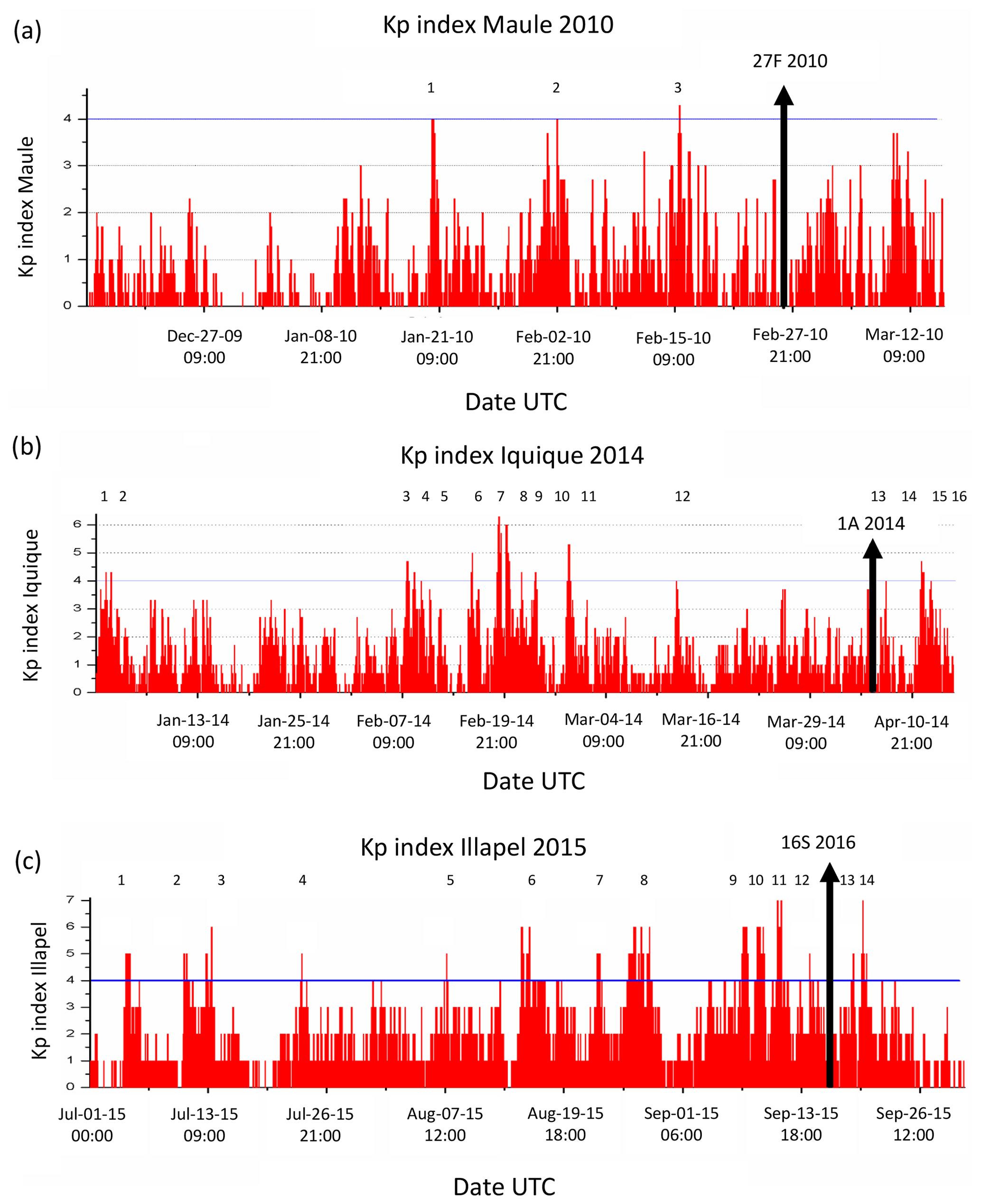
Figure 2 The Kp magnetic activity index for the periods prior to the Maule 2010 (a), Iquique 2014 (b), and Illapel 2015 (c) earthquakes (NOAA SPIDR) (WDCFG, Kyoto University).

3 Main magnetic evolution and frequency analysis

Magnetic measurements and analysis are presented in this section. The main aim of this section is to use different magnetic methodologies and figure out which of them seems more earthquake-related. The stages correspond to the long-term magnetic evolution, the simple frequency analysis, and wavelet and anomaly analysis. Stations used here are Putre (PUT), Easter Island (IPM, also known as Isla de Pascua), Los Cerrillos (CER), Pilar (PIL), Osorno (OSO), and Laboratorio Antártico de Radiación Cósmica (LARC). See Fig. 1 for their locations, and information on PUT, CER, and LARC is in Table 1. In the case of PUT and IPM, the Dobrovolsky area and the earthquake distances will be used in the following subsections (Table 2).

Table 1 The main characteristics for the detectors of Chilean network of cosmic rays and geomagnetic observatories: location, altitude, atmospheric depth, and types of detector (Cordaro et al., 2012).

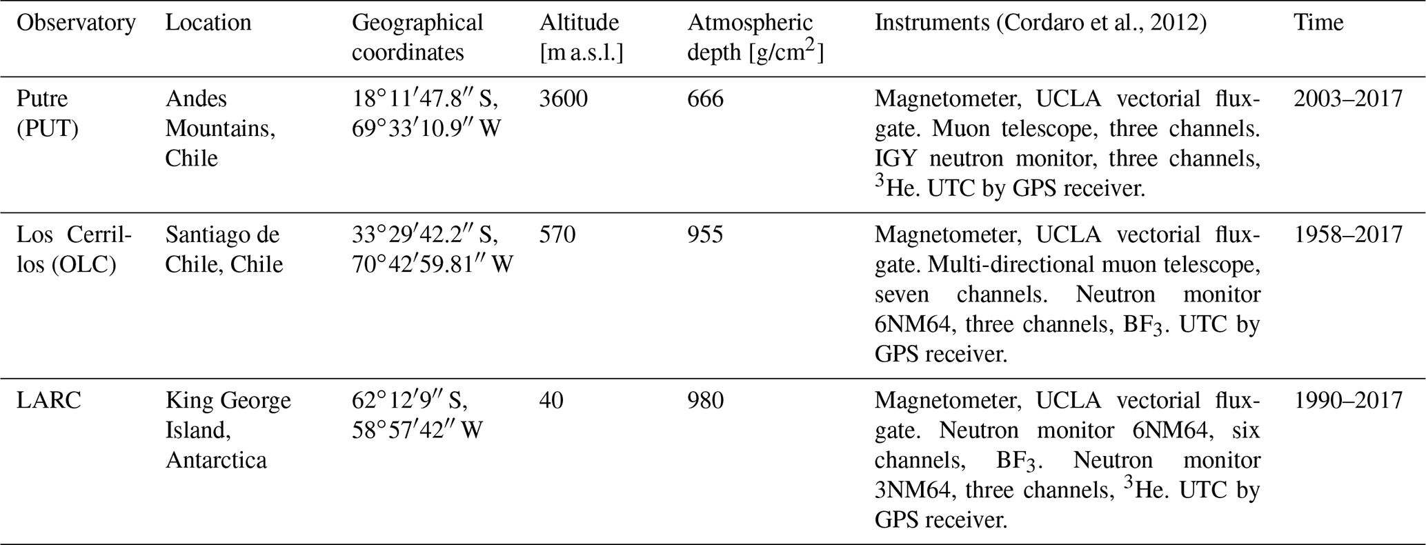
Table 2 The maximum radius where the ionosphere–lithosphere–atmosphere coupling may affect magnetic measurements corresponding to each earthquake studied at the stations of Putre and IPM (Dobrovolsky et al., 1979; Pulinets and Boyarchuk, 2004). The preparation area or Dobrovolsky area is defined by the radius r=10^0.43M, where M is the earthquake magnitude. This table shows that the Putre and IPM stations are within the earthquake preparation stage for Maule, Iquique, and Illapel.

3.1 Long-term magnetic records

A high correlation between the vertical component of the Earth's magnetic field and seismic activity at the Putre station was found (Cordaro et al., 2018). That is why we seek to specify this behavior in a shorter time window than the period studied previously (1975–2010). In addition, the B_z component in the Easter Island (IPM) station is also used because it has not been thoroughly investigated (note that the IPM station was closed in 1968 and subsequently reactivated in 2008 by the French INTERMAGNET group and the Meteorological Service of Chile) (Chulliat et al., 2009; Soloviev et al., 2012). The Putre observatory is at 18^∘11^′47.8 S, 69^∘33^′10.9 W, 3598 m a.s.l. (meters above sea level); and it is located on the western edge of the South American Plate. This zone includes the South Atlantic Magnetic Anomaly (SAMA), the center of which is 1700 km east of this observatory. The measurements confirm low B_z values at the station of Putre. The instrument error in the geomagnetic measurements is of the order of 5 nT (Cordaro et al., 2012). IPM is located at 27.1^∘ S, 109.2^∘ W, 82.83 m a.s.l., on the western edge of the Nazca Plate, characterized as a hotspot (e.g., Vezzoli and Acoocella, 2009). OSO is located at the coordinates 40^∘20^′24^′′ S, 74^∘46^′64^′′ W, and PIL is at 31^∘40^′00.0^′′ S, 63^∘53^′00.0^′′ W (Fig. 1).

In Putre, a diminution in the values of the whole magnetic field and each of its components is found. This can be attributed to the fact that the Putre observatory is influenced by the South Atlantic Magnetic Anomaly, while on Easter Island the influence of SAMA is weaker (Storini et al., 1999). These magnetic influences are also found at the Los Cerrillos observatory. The scientific and technical characteristics of the Putre (PUT) and Los Cerrillos observatories, i.e., location, altitude, atmospheric depth, type of detectors, geomagnetic cutoff rigidities, and operating times, may be found in Cordaro et al. (2012, 2016), while for Easter Island (IPM) the information is available in the SuperMAG network (Chulliat et al., 2009; Gjerloev, 2012). The main characteristics for the observatories, i.e., location, altitude, atmospheric depth, type of detector, and operation time, are shown in Table 1.

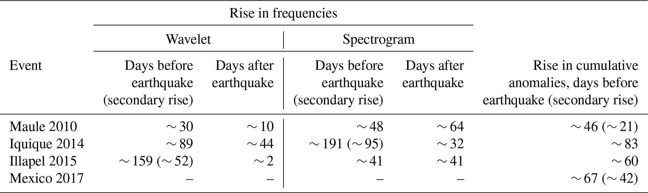
Table 3 Days before and after each frequency or anomaly rise for each earthquake considered (Maule 2010, Iquique 2014, Illapel 2015, and Mexico (Puebla) 2017 for anomalies).

Measurements of the B_z component are represented in Fig. 3. We observe similar gradients in Iquique 2014 and Illapel 2015 to those found in Maule 2010, giving rise to a jump in each case. It is known that these magnetic signals are generated by the Earth's core and disseminated through the mantle, implying changes in the mantle's electrical conductivity (Stewart et al., 1995).

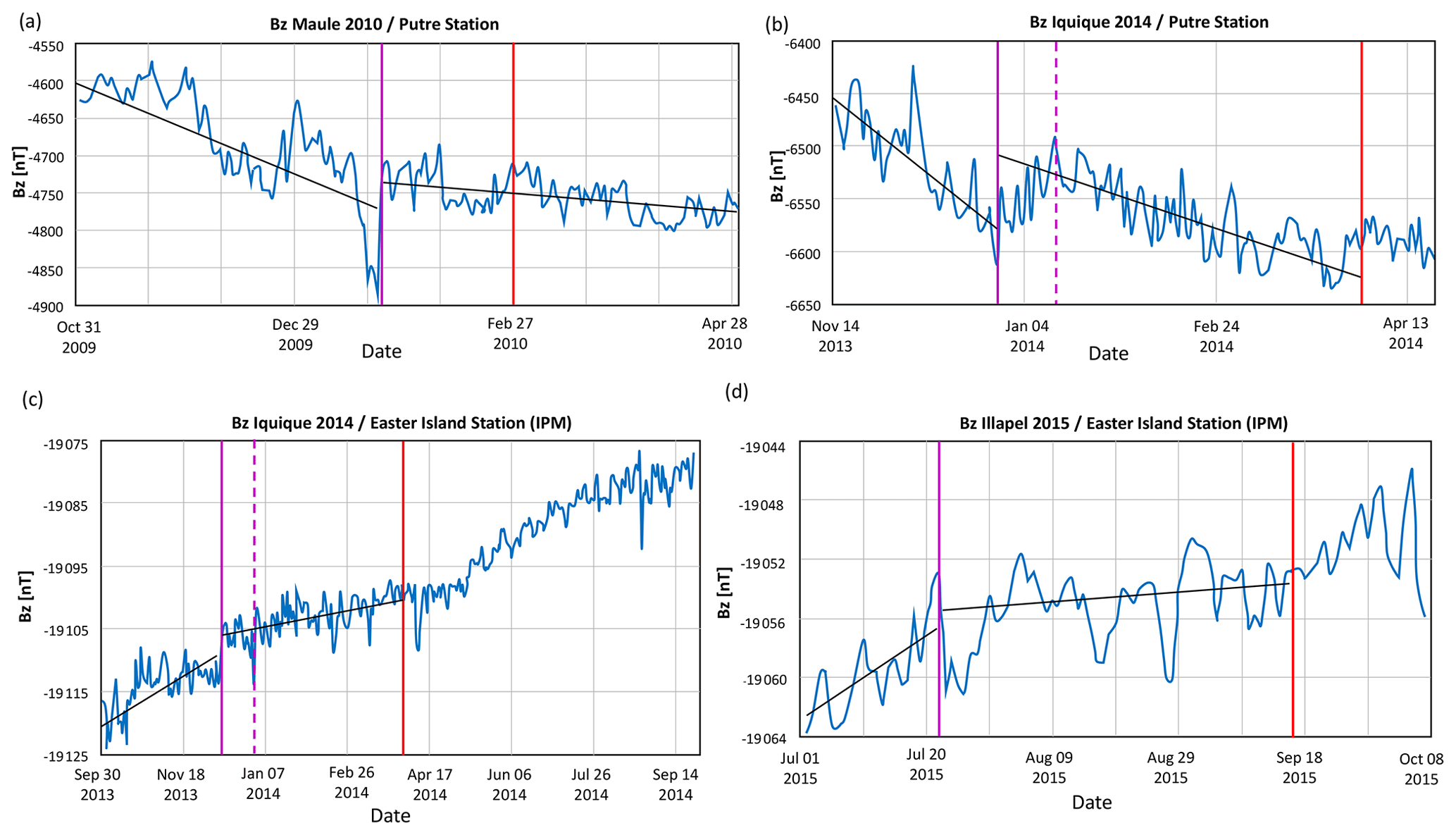
Figure 3 Vertical component B_z as a function of time at Putre and IPM stations: (a) Maule 2010 at the Putre station, (b) Iquique 2014 at the Putre station, (c) Iquique 2014 at the Easter Island station, and (d) Illapel 2015 at Easter island station. Trend changes are observed in the four cases.

The jump in the B_z component for Maule 2010 was recorded in the Putre station on 23 January 2010 (solid purple line in Fig. 3a), a time lapse of 36 d before the earthquake (solid red line) and the moment at which a change appears in the gradient or trend. It alters from a diminution of 225 nT in the period of 31 October 2009 to 23 January 2010 to a less abrupt diminution of 30 nT between 23 January 2010 and 3 April 2010; prior to the jump on 16 January 2010, there is a small, abrupt diminution from −5048 to −4927 nT. Discounting this small, abrupt diminution, the ΔB_z value between the gradients falls from −4960 to −4926 nT, Δ= 34 nT, as shown in Fig. 3a.

For Iquique 2014 the jump recorded in Putre (Fig. 3b) occurred on 27 December 2013 (solid purple line), a time lapse of 96 d before the earthquake (red solid line). A change appears in the gradient on this date from a diminution of 123 nT in the period 14 November 2013 to 27 December 2013 to a diminution of 113 nT between 27 December 2013 and 15 April 2014; the jump presents a change from −7355 to −7235 nT, Δ = 120 nT, as shown in Fig. 3. For Iquique 2014 the jump measured at IPM occurred on 31 December 2013, a time lapse of 91 d before the earthquake (Fig. 3c). The trend shows a slight increase between 30 September 2013 and 3 January 2014, from −19 116 to −19 104 nT, while a further slight increase occurs in the period of 3 January 2014 to 6 May 2014, from −19 101 to −19 099 nT. Note that the size of the jump was −3 nT, as shown in Fig. 4. For Illapel 2015 the jump measured at IPM occurred on 31 August 2015, a time lapse of 16 d before the earthquake. The trend shows a slight diminution between 31 August 2015 and 20 September 2015, from −19 054 to −19 072 nT, a jump of −11 nT, as one can observe in Fig. 3d.

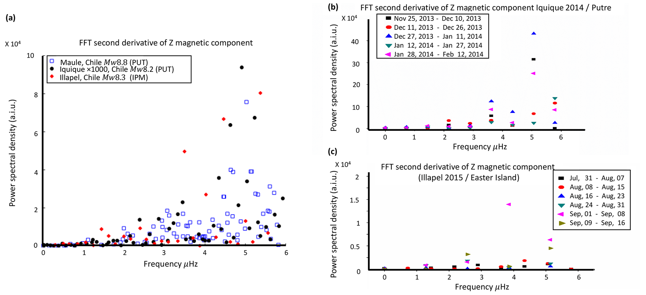
Figure 4 (a) Fast Fourier transformation (FFT) of the second derivative B_z component at Putre station for different events: Maule 2010 and Iquique 2014. The rise in frequencies in the range of microhertz are compared to the FFT of the second derivative at IPM station for Illapel 2015. (b) FFT every 15 d for Iquique 2015 at the Putre magnetometer. (c) FFT every 8 d for Illapel 2015 at the Easter Island magnetometer.

3.2 Simple Fourier analysis

Regarding the frequency analysis, the frequency spectrum values were analyzed for the Maule, Iquique, and Illapel earthquakes using the second derivative of the vertical component at PUT and IPM stations. Fundamental frequencies before these earthquakes ranged from 5.606 to 3.481 µHz or from one cycle/48.9 h to one cycle/79.13 h (Fig. 4a). The increase in one frequency or a group of frequencies reflects the oscillations of the radial magnetic field whose oscillation period takes from ∼ 2 to ∼ 4 d. Specifically, in the Maule event, peaks for the frequencies 4.747, 5.064, and 5.154 µHz were recorded (blue squares in Fig. 4a). In Iquique peaks of 4.611, 4.882, and 5.154 µHz were recorded (black dots in Fig. 4a), and for Illapel, 3.739, 4.630, and 5.520 µHz were recorded (red rhombuses in Fig. 4a).

In order to identify a temporal domain where these frequencies arise, FFT is applied every 20 d as a first approximation (Fig. 4b, c). Before the Iquique 2014 event a jump in intensity was observed that was associated with the frequency of 5.154 µHz for the period 27 December 2013 to 11 January 2014, i.e., after the jump (Figs. 3b, 4b). Similar frequencies (3.739 µHz) rise during 1 to 8 September 2015 before the Illapel 2015 event (Fig. 4c). These findings imply a more detailed methodology is required in order to study the origin of these frequencies.

3.3 Wavelet analysis

We have used the wavelet transformation to analyze localized versions of power within a geomagnetic time series. In this way, it can break down a time series into time–frequency space and determine the dominant modes of variability and how they vary over time (Torrence and Compo, 1998). Here, the goal is to look for the rare variations that could not be attributed to space weather in the daily average measurements. According to Cordaro et al. (2018), the magnetic field's vertical component showed variations related to the Maule 2010 earthquake. That is why values of the vertical component of the geomagnetic measurements at the OSO station were considered. Note that the OSO station is the closest station to the main earthquake. In order to avoid space weather influence, the highest variations were not considered. One way to consider these two restrictions is by using statistical analysis. For example, a lower and upper threshold could be defined by using the standard deviation. Consider the higher magnetic peaks, but they are not too meaningful because they could be related to space weather conditions. An example of this statistical analysis when an upper threshold of 2 standard deviations is used can be found in Fig. 5, in which panels (a), (b), and (c) represent the Maule 2010, Iquique 2014, and Illapel 2015 earthquakes, respectively. For Maule 2010, the spectral analysis shows a dramatic increase 30 d before the Maule earthquake and a decrease 10 d after the earthquake occurrence (yellow and green arrows in Fig. 5a). The frequencies that rise comprise a range close to 3–5 µHz. Note that no other significant increase is seen during the 2 years of measurements between days −365 up to −30, and between days 10 and 365 it is clear that there is no significant rise in frequencies (blue shading in Fig. 5a). Panel (b) of Fig. 5 shows the results for Iquique 2014, which is characterized by two peaks. The first one rises 89 d before the earthquake (yellow arrow in Fig. 5b), while the second one occurs after the Iquique earthquake (after the red line, which indicates the earthquake day). The Illapel case is also characterized by two peaks, as shown in panel (c) of Fig. 5. The first rise occurs ∼ 159 d before the earthquake (yellow arrow in Fig. 5c), while the second rise is 52 d before the main earthquake (grey arrow in Fig. 5c). Despite this promising methodology that considers the daily average and the upper threshold, an improved implementation of physical (i.e., space weather conditions) and statistical (adequate definition of anomalies and frequency considerations) analysis is required.

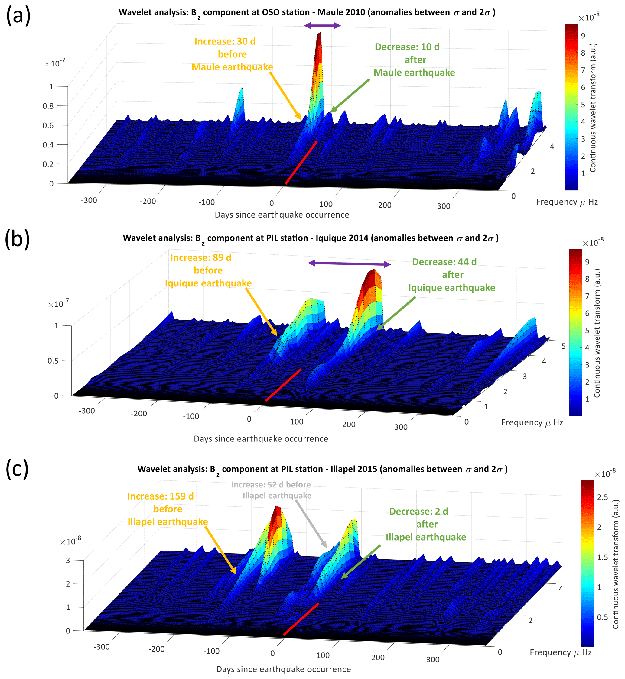
Figure 5 Wavelet for B_z at OSO station is shown. These graphs are obtained by restricting the peaks considered in a band and daily average values during 2 years of measurements. The wavelet spectrum shows an increase prior to and after the Maule earthquake. Unlike the spectrogram method where it is enough to consider the anomalous peaks above a threshold, wavelet analysis is more complex to calibrate than spectrogram analysis (upper limit).

Finally, let us point out that more profound and sophisticated multiresolution wavelet analysis on time series related to earthquakes has been performed by Telesca et al. (2004, 2007). This kind of study will be considered in future works.

3.4 Anomaly analysis

In order to identify and discriminate external variations from those that could be considered lithospheric (variations with lithospheric origin), this subsection handles the definitions of anomalous variations. This definition will be obtained considering the external perturbation by using the Dst index (http://wdc.kugi.kyoto-u.ac.jp, last access: 7 June 2021). Then spectral analysis will be performed. Additionally, the data used in this subsection are standard and come from the SuperMAG network (http://supermag.jhuapl.edu/, last access: 7 June 2021). The data have a sampling frequency of one datum per minute, and a period of 1 year before and 1 year after each earthquake was chosen.

3.4.1 Magnetic threshold definition

In the method of cumulative magnetic anomalies on the surface of Earth, we used statistically atypical or anomalous values, that is, data that are quite far from the average values of the sample. So, we compare real values of B_i with a more representative value of the sample, its average ${\overline{B}}_i$. We will call the difference between the two the magnetic residual ΔB_i. By using the distribution of data, we can define when a value is atypical or anomalous in a normal distribution by statistical definitions of quartiles and outliers.

On the one hand, we create a filter that eliminates the frequencies averaged near Nyquist and establishes a filter that eliminates high frequencies (stochastic filter). The option was to consider a weighted moving average of five points: ${\overline{B}}_i=a{B}_{i-\mathrm{2}}+b{B}_{i-\mathrm{1}}+c{B}_i+b{B}_{i+\mathrm{1}}+a{B}_{i+\mathrm{2}}$. Here, other researchers have used cubic splines instead of moving averages (e.g., De Santis et al., 2017). In our case we use a=0.07, b=0.25, and c=0.5–2a. The uncertainty in the fluxgate magnetometers (SuperMAG) from OSO and PIL stations is $\mathit{\delta }{B}_i=\pm \mathrm{0.1}$ nT, while the error in the moving average implementation is $\mathit{\delta }{\overline{B}}_i=\pm \mathrm{0.1}$ nT. As residual values are defined as the difference between real and smoothed data ($\mathrm{\Delta }{B}_i=B_i-{\overline{B}}_i$), the total error propagation of the residual is $\mathit{\delta }{B}_i+\mathit{\delta }{\overline{B}}_i=\pm \mathrm{0.2}$ nT.

Let us comment that the error in propagation is used to define a threshold that determines when a residual is considered anomalous or not. For instance, in statistics 0.6745σ represents the 50 % of the data that are closer to the average (where σ is the standard deviation). This means that residuals less than 0.6745σ nT are closer to the average and therefore are more common. As residuals are considered anomalous when they are unlikely, anomalous data should be defined as those residuals larger than 0.6745σ nT. By adding the error propagation as a condition (0.6745σ+0.2 nT) and considering that the standard deviation is similar to σ∼0.1 nT, the percentage of residuals that meets this condition is considerably smaller than the 50 % of the data (less common). Thus, residuals ΔB_i are considered anomalous (ΔB_ai) when

$$\begin{array}{}\text{(1)}& \left|\mathrm{\Delta }{B}_i\right|\ge \mathrm{0.6745}\mathit{\sigma }+\mathrm{0.2}\mathrm{nT}.\end{array}$$

The vertical magnetic thresholds found are 0.2246995 nT at OSO (27 February 2009–27 February 2011), 0.2362868 nT at PIL (1 April 2013–1 April 2015), and 0.2352825 nT at PIL (16 September 2014–16 September 2016). These threshold are ∼ 6, ∼ 4.5, and ∼ 4.5 times larger than each respective σ. This means that each anomaly above this threshold meets the 3σ criterion (a valid observation). Furthermore, the thresholds are close to the 5σ criterion which corresponds to the standard discovery criteria in the physical sciences; for example this criterion was used in the discovery of the Higgs boson (https://home.cern/news/news/physics/higgs-within-reach, last access: 7 June 2021).

Regarding the external contribution, the data considered are for quiet periods, $\left|\text{Dst}\right|\mathit{<}\mathrm{10}$ nT, and only quiet magnetic data between 16:00 and 05:00 local time are considered (Hitchmn et al., 1998). Some researchers who have used satellites consider only the time periods in which the Dst index is less than or equal to 20 nT (e.g., Marchetti and Akhoondzadeh, 2018) or equal to 10 nT (e.g., De Santis et al., 2017). That means that the space weather conditions could invalidate the anomaly condition defined in Eq. (1) if $\left|\text{Dst}\right|\mathit{>}\mathrm{10}$ nT. Then, the proper application of Eq. (1) is linked to those times where space weather activity is low. That is when $\left|\text{Dst}\right|\mathit{<}\mathrm{10}$ nT and magnetic data are quiet (16:00 to 05:00 local time).

Finally, the fourth filter process considered corresponds to the study of the recurrence of anomalous residuals. For instance, if the anomalous threshold is 3 times the standard deviation, it implies that 1 datum of every 740 data is anomalous. This is the same as 2 every 1480. As this work uses 1440 data per day, it is expected that ∼ 2 will be anomalous per day. In terms of probabilities, this is the same as P_day≈0.0014. Contrarily, if 1 single day shows, let us say, 30 anomalies, the probability is $P_{\mathrm{30}}={\left(P_{\mathrm{day}}\right)}^{\mathrm{30}}\sim {\mathrm{10}}^{-\mathrm{86}}$. This means that the occurrence of 30 anomalies is virtually zero, and it could imply that the previous filters (anomaly definition, Dst, and quiet time) failed during that day. Then, it is not possible to consider those days where the number of anomalies per day is considerably larger than 2. That is why days with more than 10 anomalies are not considered valid.

3.4.2 Spectrogram

The filtered data correspond to a strong candidacy of lithospheric magnetic origin. This means that any spectral analysis could reveal lithospheric variations. That is why simple spectrogram analysis is performed. The spectrogram corresponds to the application of the moving Fourier transform. Here, the temporal window size is 1 month with a 50 % overlap, which corresponds to a reasonable spectral and time resolution (see Rabiner and Schafer, 1980, and Oppenheim et al., 1999, for spectrogram theory and application). The OSO and PIL spectrograms for Maule 2010, Iquique 2014, and Illapel 2015 are shown in Fig. 6.

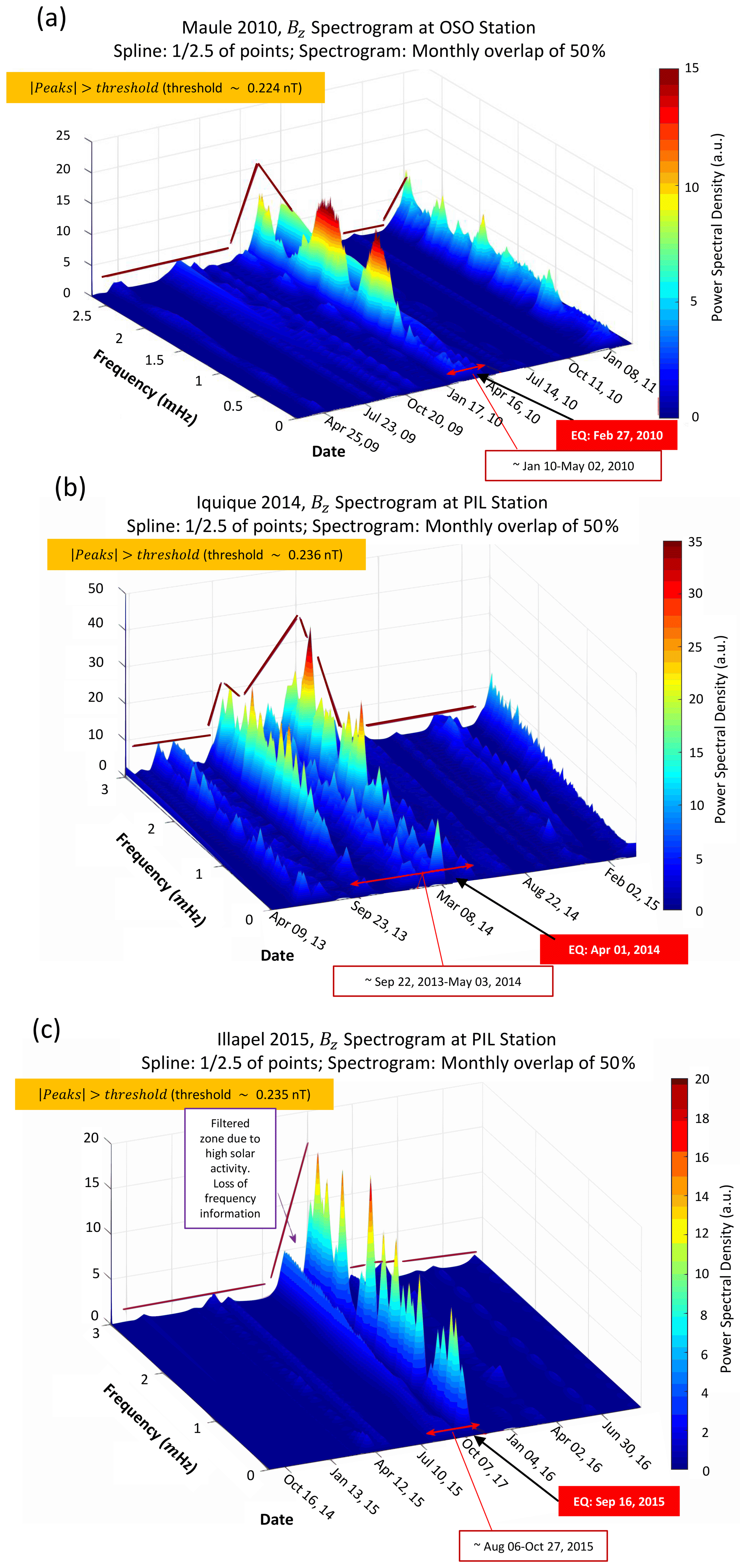
Figure 6 Spectrogram analysis of vertical magnetic components after the external influence is filtered. (a) The rise in a range of frequencies (1–2.5 mHz) appears prior to and after the Maule 2010 earthquake (OSO station). The active frequencies last less than 3 months. (b) The rise in similar frequencies appears prior to the Iquique 2014 earthquake in the vertical component of the PIL station. This frequency activity lasts more than 5 months. (c) The solar events are intense during September 2015. Nevertheless, this can be seen as an increase in the spectrum since August 2015. This frequency activity lasts close to 3 months. Three earthquakes hit when the rise in ultra-low frequencies (mHz) exists. Note that Iquique is not filtered by Dst as Maule and Illapel are.

In the Maule 2010 event, the spectrogram of the vertical magnetic component at the OSO station is shown in Fig. 6a. There is no significant rise in frequencies during the period before the Maule event (before ∼ 10 January 2010). Nevertheless, a dramatic increase during the period 10 January–2 May 2010 occurs. Specifically, the rise in frequencies lies in the range ∼ 1–2.2 mHz. The onset of this rise (10 January) occurs more than 1 month before the Maule earthquake (27 February) and lasts almost 4 months. That means that the spectral density reduces their activity after ∼ 2 months of the earthquake.

The spectrogram for Iquique 2014 is characterized by two peaks (Fig. 6b). The first one corresponds to 22 September 2013, and the second one corresponds to ∼ 8 March 2014. Here, the frequency range comprises between ∼ 1.2 and 2.7 mHz, which is similar to that found in the Maule spectrogram. However, the main peak occurred during March, which is characterized by a dominant frequency close to 2.5 mHz, while the dominant frequencies in Maule 2010 are close to 1.2 and 2.2 mHz. There is an additional difference compared to the Maule event: the rise in frequencies in Iquique 2014 comprises a significant decrease (or “valley”) in the spectral density, which lasts almost 2 months (∼ 9 November–27 December 2013). It means that the second rise in frequencies lasts more than 4 months (∼ 27 December 2013–3 May 2014), which is a similar duration compared to the frequency rise of Maule 2010.

The final spectrogram is found in Fig. 6c, which corresponds to the Illapel 2015 event. Here, it can be seen that almost the entire period was characterized by close-to-zero frequency variations. Nevertheless, the frequency rise is similar to that obtained in Maule 2010. That is, significant frequencies rise only on dates close to the earthquake event. The rise lasts almost 3 months (∼ 6 August–27 October 2015). It is important to note that the gap in September 2015 is due to the strong spatial weather activity. Despite this, it is clear that the earthquake occurrence is during periods of high-frequency activity, which is a similar feature compared to Maule 2010 and Iquique 2014.

Panels (a)–(c) of Fig. 6 show that three strong earthquakes (Maule 2010, Iquique 2015, and Illapel 2015, respectively) occurred during the rise in ultra-low frequencies of the vertical magnetic component. It is important to highlight that these frequencies (mainly 1–2.5 mHz) vanish or reduce their intensity values during other time periods. This is in agreement with other authors who have claimed that accompanying ultra-low frequencies (e.g., Contoyiannis, et al., 2016; Han et al., 2020) and the increases in the number of magnetic anomalies are related to the earthquake preparation process (e.g., De Santis et al., 2017). It means that anomalous peaks produce the magnetic oscillations in the magnetic records. By following the Venegas-Aravena et al. (2019) findings, the number of these peaks should also increase (decrease) in time before (after) earthquake occurrences.

3.4.3 Cumulative daily anomalies

By following the anomaly definition (Sect. 3.4.1), it is possible to find the daily number of anomalies. For example, in Fig. 7 the case of the OSO station is shown. Black dots follow a stable linear increase in the number of cumulative anomalies (red line). Nevertheless, this tendency breaks close to 11–12 January 2010. From those days up to the first week of April, the numbers of anomalies experiences a dramatic increase. In the middle of this increase, the Maule earthquake hits (27 February 2010). By subtracting the initial linear tendency and comparing it to the PIL station (Iquique 2014 and Illapel 2015), the sigmoidal feature is clearer (Fig. 8). The anomalies start to increase prior to each earthquake. For example, this increase started ∼ 47 d before the Maule 2010 earthquake, ∼ 90 d before the Iquique 2014 earthquake, and ∼ 60 d before the Illapel 2015 earthquake (Fig. 8).

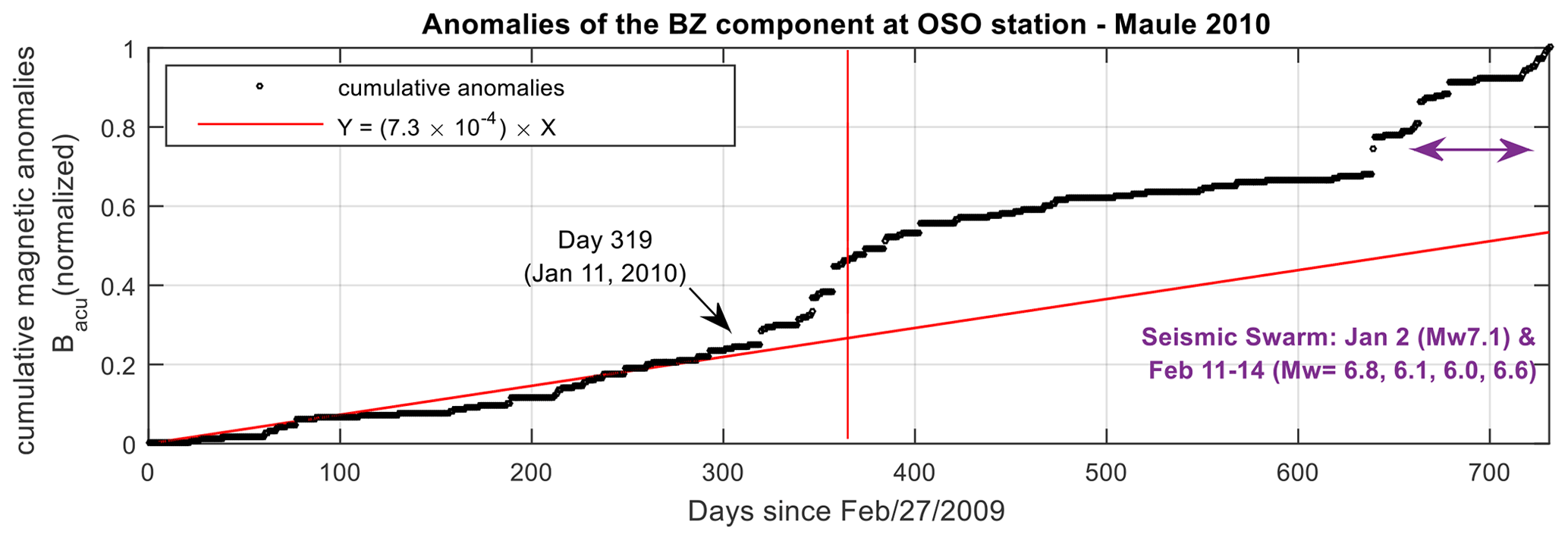
Figure 7 Accumulated magnetic anomalies of B_z and a linear interpolation in the period of 2 years starting on 27 February 2009. The data were taken at the OSO station. Close to the main earthquake, the linear trend breaks and the number of anomalies increases. Other important seismic events hit near the stations during the last period. Nevertheless, it is not clear that the anomaly increases are due to these specific events.

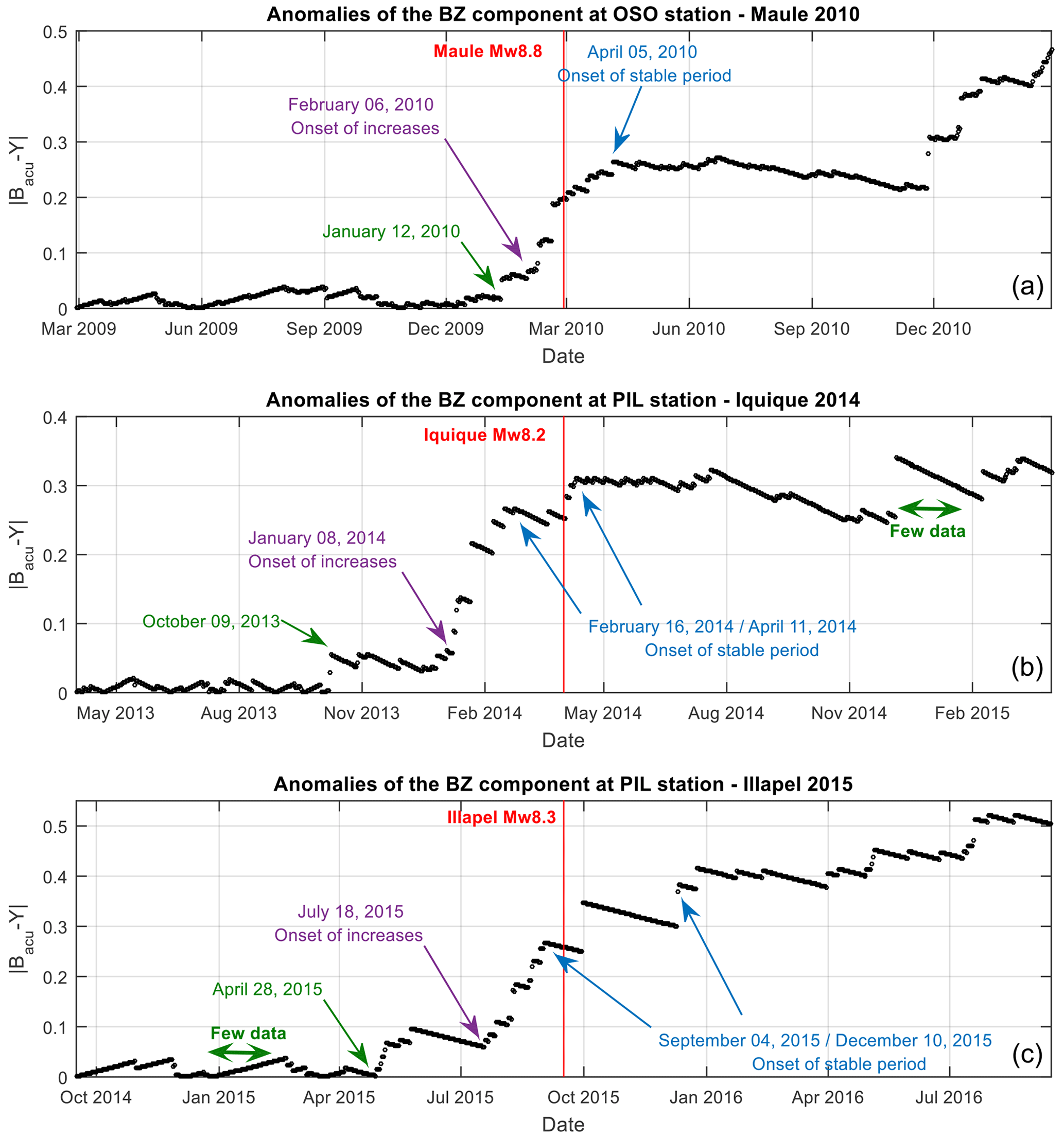
Figure 8 Variation in the accumulated diary of magnetic anomalies of B_z during 2 years close to the three earthquakes: (a) Maule, (b) Iquique, and (c) Illapel. The data were taken at OSO station (a) and PIL station (b, c), respectively. Is clear that the sigmoidal shape is similar in all of the earthquakes. This means that these stations recorded a dramatic increase in the number of magnetic anomalies between 50 and 90 d prior to each earthquake.

Other researchers have used very different implementations, definitions, methodologies, and data in order to find these anomalies. For example, Marchetti and Akhoondzadeh (2018) have also found a sigmoidal signature in the anomalies of the Y components recorded by different satellites for the Mexico (Puebla) 2017 earthquake. In order to compare Mexico 2017 with Maule 2010, Iquique 2014, and Illapel 2015, the initial linear trend has been removed (Fig. 9). The initial onset of anomalies increased close to 60 d prior to the Mexico 2017 earthquake. Note that in the four cases, the sigmoidal features are almost the same: a linear stable number of anomalies characterize the initial period. Then a dramatic increase in the number of daily anomalies is followed by the main earthquake. This time is different in each earthquake but it lies between 50–90 d after the initial anomalies increase. After the seismic events happen, the cumulative numbers do not behave similarly. For example, in the Mexico 2017 earthquake, the anomalies remain stable, while in the Maule 2010 earthquake they still increase but in a less dramatic manner. At the end of the OSO measurements, several anomalies appear, but it is not clear whether these events could be related to other seismic events. In order to understand the physics that lies in these events, a theoretical mechanism is required.

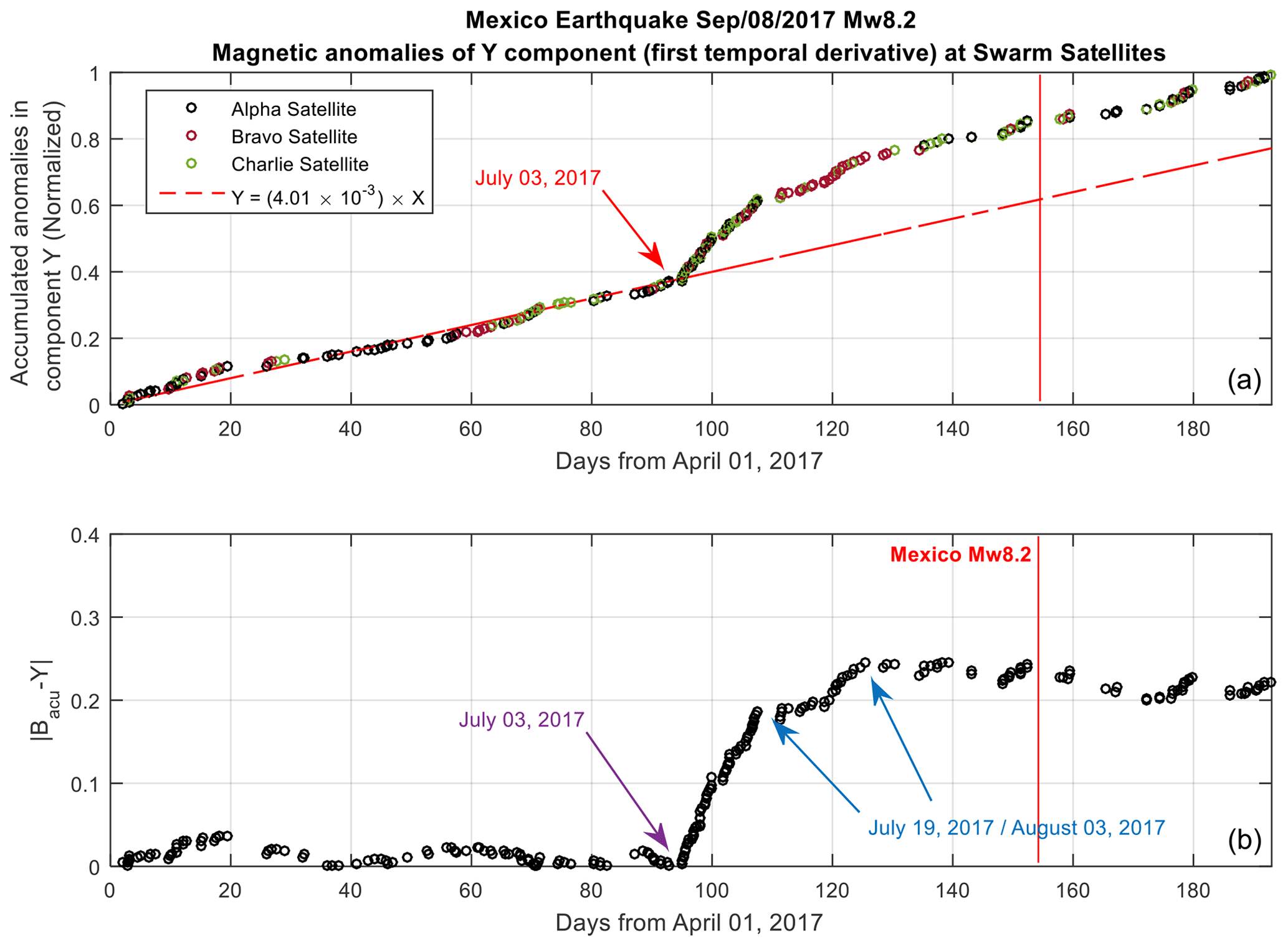
Figure 9 (a) Accumulated diary of magnetic anomalies during 2 years, in component Y from 1 April to 15 October 2017 for the Mexico earthquake of 8 September 2017, M_w 8.2. (b) Residual behavior of Mexico earthquake. The data are open source and were taken from the swarm project (https://swarm-diss.eo.esa.int/, last access: 7 June 2021). Methodology was developed by Marchetti and Akhoondzadeh (2018).

4 Magnetic anomalies and fracture mechanics by considering the seismo-electromagnetic theory

The frequency analysis (Figs. 5, 6) and cumulative number of magnetic anomalies (Figs. 7, 8, 9) show an increase (spectral intensity and anomalies number) before each earthquake occurs. In the anomalies case, a clear sigmoidal feature rises in Maule, Iquique, and Illapel, which is similar behavior to that recorded in the Mexico earthquake (Fig. 9; Marchetti and Akhoondzadeh, 2018). This indicates that anomaly behavior could correspond to a lithospheric origin. Currently, it has been shown that the origin of these anomalies is associated with the cracking (or microcracking) of the semi-fragile–ductile part of the lithosphere (crust) due to changes in stress (Venegas-Aravena et al., 2019). Typically, strain appears when solids undergo loads or stress accumulation. However, microcracks rise specifically when solids cannot contain more deformation and prior to the main failure (e.g., Stavrakas et al., 2019; Li et al., 2020). Experimentally, it has been shown that these conditions break the electrical neutrality within materials and generate an electrical flux through rocks in a process known as pressure-stimulated currents or PSCs (e.g., Anastasiadis et al., 2004). Furthermore, it has been shown that PSCs can explain that the fractal nature of cracks is sufficient to generate the frequency spectrum, co-seismic variations, anomalies and their behavior, and variation in the ionosphere in a theory known as seismo-electromagnetic theory (Venegas-Aravena et al., 2019). Regarding the time evolution of magnetic anomalies, De Santis et al. (2011) have shown that the sigmoidal shape is due to a manifestation of the stress changes when it reaches a critical point. Nowadays, theoretical development, geodynamical measurements, and experimental studies have shown that the sigmoidal shape appears as a consequence of the dramatic increase in the number of microcracks (at a depth of a few tens of kilometers) prior to the main earthquake ruptures (De Santis et al., 2015; Stavrakas et al., 2019; Venegas-Aravena, et al., 2019).

A schematic representation of the crack generation in the geodynamical context can be seen in Fig. 10. At the initial time t=t₀, the intact lithosphere undergoes a uniaxial non-constant stress σ (Fig. 10a). Then the first signs of microcracks appear at t=t₁ due to the increase in the stress (Fig. 10b). When the lithosphere cannot withstand more deformation, a dramatic increase in the crack generation appears throughout the lithosphere (t=t₂ in Fig. 10c). At this point (t=t₃ in Fig. 10d), the crack generation is not sufficient to release the excess of uniaxial stress. Then the lithosphere cannot release energy by either deformation or the crack generation mechanism. That is why the rupture (earthquake) occurs (green area in Fig. 10d) at t=t₄. After the main rupture, another aftershock occurs (smaller green patches within the fault in Fig. 10e). Nevertheless, the number of anomalies starts to decrease. Finally, the microcrack generation stops because the deformation is sufficient to handle the lithospheric response to non-constant uniaxial stress (Fig. 10f).

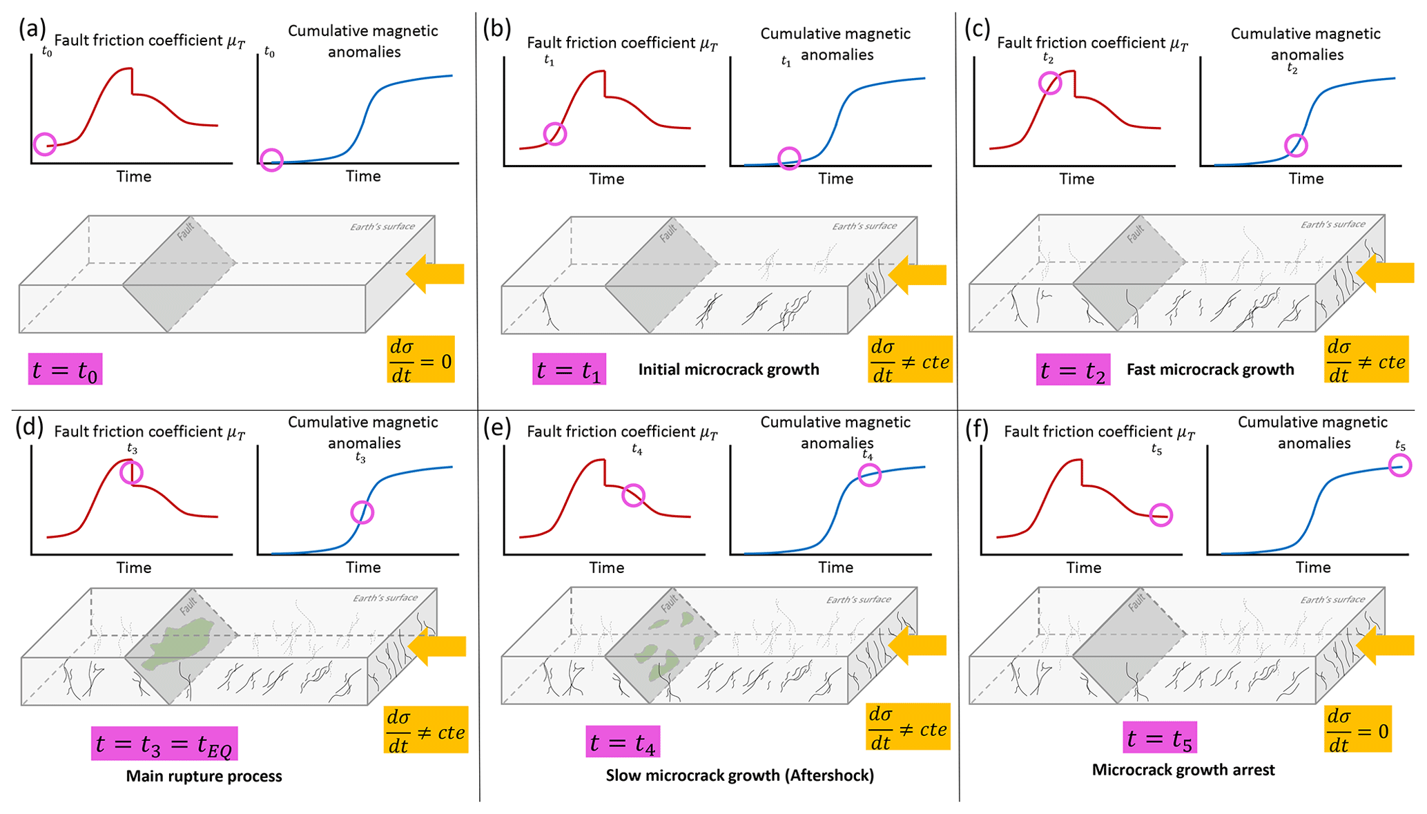
Figure 10 Schematic representation of the seismo-electromagnetic theory. The anomalies generation are owing the creation of several microcracks. The number of cracks increase because the internal collapse of the lithosphere when a non-constant uniaxial stress is applied.

Additionally, Venegas-Aravena et al. (2019) found that the increase in the number of anomalies is controlled by the same fractal nature that drives the microcrack generation. This means that the frequency of the electrical flux could cover several magnitude orders. For example, Figs. 4, 5, and 6 are characterized by the rise in different frequencies (micro- to millihertz), which are known as ultra-low frequency (ULF), prior to the main earthquakes. These frequency ranges were also found and described in other research such as that of Fenoglio et al. (1995), Vallianatos and Tzanis (2003), Fraser-Smith (2008), De Santis et al. (2017), and Cordaro et al. (2018).

Finally, it has been concluded that there must be precursory magnetic anomalies of the order of 0.1 nT related to earthquakes on the Earth's surface (e.g., De Santis et al., 2017; Chernogor, 2019; Venegas-Aravena et al., 2019). In the previous section, it was found that the minimum value to define an anomaly was close to 0.2 nT. Therefore, this experimental result is in agreement with the theoretical value obtained. Consequently, as the seismo-electromagnetic theory indicates, those magnetic anomalies may have a lithospheric origin. Furthermore, the behavior of all these anomalies features a preceding increase similar to that of other seismic events that use different data and methods (e.g., De Santis et al., 2019a, 2019b, and references therein).

5 Discussions and conclusions

The most significant characteristics of the magnetic field and its variations are found in the z component, which we have observed and recorded at the Putre and IPM observatories. The previous measurements show that there is evidence of a progressive increase in the phenomenon known as the South Atlantic Magnetic Anomaly (SAMA) (Cordaro et al., 2019). As expected, it generates a significant deviation in the intensities present in the OP station as shown in the magnetic iso-values (Fig. 1). Combining this information with data from the IPM station, the behavior of the radial component of the geomagnetic field for the three most significant seismic events in the Chilean Pacific sector during the period 2010–2015 was recorded, and it corroborates the magnetic relation with seismology shown in Potirakis et al. (2016), Contoyiannis et al. (2016), and De Santis et al. (2017), who used other methods.

The normal magnetic trend showed some long-term variations. For example, there were breaks in the trend or a jump in B_z, followed by a time lapse and seismic movement as one can observe in Fig. 3. These jumps occur in different forms: in Putre they are significant, reaching values of tens of nanoteslas, while in IPM the jump is barely 10 nT. The time lapse between each jump and the seismic event differs in each event. For Maule 2010 it was 36 d; for Iquique 2014 it was 96 d, and for Illapel it was 16 d. This time difference may be due to an important factor: it appears that the jump is not equally strong in the three events, since the jump before the Iquique 2014 event was considerably weaker than the one before Illapel 2015 and preceded the event by a longer time lapse (96 d). The more abrupt jump recorded in Illapel was followed by a shorter time lapse (16 d). These changes are notorious, which is why a first approach using frequency analysis was made.

Specifically, significant frequency data obtained for the Maule 2010 earthquake, Chile; the Tōhoku 2011 earthquake, Japan; and the Sumatra–Andaman 2004 earthquake, Indonesia, range from 4.747 to 5.154 µHz, from 4.747 to 5.606 µHz, and from 3.481 to 5.425 µHz, respectively (Cordaro et al., 2018). These fundamental frequencies were detected before the earthquakes in the areas of the Pacific Ocean in the Southern Hemisphere and the Eurasian (2011) and Philippine (2004) areas in the Northern Hemisphere. Now these significant frequencies have been obtained again in different places and at different times on Earth: for Iquique 2014, peaks of 4.611, 4.882, and 5.154 µHz and for Illapel 2015, peaks of 3.739, 4.630, and 5.520 µHz (Fig. 4). Up to this point, the rise in these frequencies could be thought of as normal magnetic behavior with a high degree of coincidence. That is why other methodologies were used in order to clarify the origin of these frequencies.

In order to avoid bias or technical malfunction, we have decided to use different stations that belong to an international network with open-source data (SuperMAG). These stations (OSO and PIL) were the closest to the three earthquakes that had continuous measurements. The time period was 1 year before each earthquake and 1 year after, giving 6 years of combined measurements where the frequency sample was one datum per minute.

The first approach was performed by using wavelet analysis at the OSO station. Here, in order to avoid normal variations and external perturbation, daily average values were performed by imposing a lower and upper restriction before applying wavelet analysis. Fig. 5a shows the increase in the frequency range (>2 µHz) ∼ 30 d before the Maule 2010 earthquake. These frequency activities last for up to ∼ 10 d after the earthquake. Similar frequency results were obtained for Iquique 2014 (Fig. 5b) and Illapel 2015 (Fig. 5c). Despite the abovementioned results, the previous restrictions might be seen as arbitrary. That is why we moved to a stricter, stronger, and bias-free methodology. Besides, three facts should be taken into account. The first one is considering the physics-based filter processes, which remove most of the noise and external disturbances. Thus, this allows performing more simple frequency analysis such as the moving Fourier transform (spectrogram). The second one is the tridimensional representation. This is important because it is possible to observe the relative frequency intensity differences in a reliable way. Furthermore, the third one is that this spectrogram and its tridimensional representation allow us to compare our results to previous works in the field (for example, Cordaro et al., 2018).

The definition of magnetic anomalies was given in Sect. 3.4.1. There the anomalous magnetic variations were defined by using statistical analysis. That is, one variation or peak will be considered anomalous if it reaches values beyond a certain threshold, a threshold that is defined by the same data. In order to avoid the external perturbations, the Dst index and quiet time were considered. This gives 6 years of combined data with variations that could be associated with the lithosphere or internal. An increase in the frequency range (∼ 1 mHz) before each earthquake was obtained after applying spectrogram analysis (Fig. 6). If we look at those periods not close to the earthquakes' occurrences, almost no frequency activity was recorded. In addition, these frequencies cannot be considered part of tidal effects because the last one belongs to a different frequency range (∼ 0.01–0.06 mHz) (Casotto and Biscani, 2004; Park et al., 2005). Prior studies have shown that the frequencies approximately in the range of millihertz are also related to the earthquake preparation stage (Zlotnicki et al., 2001). This implies that Maule 2010, Iquique 2014, and Illapel 2015 occurred during very high frequency activity comparable to that found by Zlotnicki et al. (2001). As the considered data are free of external perturbations and earthquake occurrences are within these frequencies' activations, the idea of the existence of lithospheric frequencies related to earthquakes is reinforced.

In order to compare these data with other results, we performed a count of the daily anomalies. Here, the anomalies behave as a sigmoidal function (Figs. 7, 8, 9). In all of the earthquakes a dramatic increase in the number of anomalies was found between 50 and 90 d before each earthquake. This long-term behavior is similar to that found in Nepal 2015 (De Santis et al., 2017), in Mexico 2017 (Marchetti and Akhoondzadeh, 2018), in central Italy (Marchetti et al., 2019a), in Indonesia 2018 (Marchetti et al., 2019b), or for other big earthquakes worldwide (De Santis et al., 2019b). Note that the abovementioned studies used satellite data in contrast with this study which employs ground-based magnetometers and a different methodology. Additionally, the station selection followed the preparatory phase described by Dobrovolsky et al. (1979). This means that any magnetic station close to the impending earthquake (∼ 1000 km) should detect anomalies or the lithospheric microcracking beneath the Earth's surface. The horizontal distance of the preparation phase also agrees with geodetic findings. For example, Bedford et al. (2020) found a preparation phase characterized by a high increase in the strain close to ∼ 1000 km in the subduction margin. Note that the dates when anomalies rise dramatically are 6 February 2010 for Maule and 8 January 2014 for Iquique as shown in Fig. 8. These dates match well compared to the onset of critical seismicity throughout the concept of characteristic precursory minima (β) in the framework of natural time analysis, for instance, 1 February 2010 and 28 December 2013 (Sarlis et al., 2015). In addition, Fig. 6b shows that the second (main) rise in frequencies begins on 27 December 2013. On the other hand, it is possible to observe that the onset of a second rise in the cumulative number of anomalies for the Mexico 2017 earthquake is close to day 118 (Fig. 9), which corresponds to 28 July 2017. Our date is almost the same date (27 July 2017) as that obtained by Sarlis et al. (2019) by applying the critical seismicity methods. It is then possible to claim that these similarities among frequencies, cumulative anomalies, and seismicity features should be considered different manifestations of a lithospheric phase transition.

By considering the above and the four filters applied (Dst, quiet daily time, stochastic, and recurrences) which determined the definition of residual anomalies, it is possible to explain our results in terms of the physical mechanism described in the seismo-electromagnetic theory. This scheme explains different empirical observations that indicate a direct relation between magnetic fields and earthquakes in which the essential group of measurements corresponds to the recording of ultra-low-frequency magnetic signals, mainly close to the millihertz and microhertz range (Venegas-Aravena et al., 2019, 2020). It is important to note that this theory considers the microcracking process (due to stress changes in the semi-brittle–ductile regime) a fundamental physical unit because its electrical properties (e.g., Triantis et al., 2020) or its influence on the propagation of the main failure (e.g., McBeck et al., 2021) has been widely studied. Under this concept, the anomalies correspond to the manifestation of the crack or microcrack within the lithosphere which allows the flux of electrical current due to the Zener–Stroh mechanism (e.g., Stroh, 1955; Ma et al., 2011), while changes in the seismicity rate are due to changes in the b value (Venegas-Aravena et al., 2020) which could generate seismic foreshock or slow slips as in Iquique 2014 (e.g., Herman et al., 2016). Also, this theory considers the main earthquake a crack that releases seismic energy as coseismic magnetic signals (Kanamori, 1977; Utada et al., 2011). The temporal evolution of these cracks and its relation to the sigmoidal magnetic anomalies' behavior can be seen in Fig. 10. The framework of this theory states that the microcracks appear as a consequence of the excess of shear stress that cannot be released by the lithospheric deformation (Venegas-Aravena et al., 2019). Then, frequency rise and anomaly behavior should be considered a manifestation of the internal lithospheric collapse at the last stage (preparation stage) of the seismic cycle, when solids cannot bear more strain. Since the electrical currents are intense after the linear regime (Triantis et al., 2020), the phase transition described by Sarlis et al. (2019) could be considered a (physical and statistical) manifestation of the changes in the semi-brittle–ductile regime. Then, they can generate the abovementioned magnetic anomalies found in this work.

Regarding the mechanism that generates the microcracks, we found that the minimum value to define an anomaly was close to 0.2 nT, and this experimental result is in agreement with the theoretical value obtained in Venegas-Aravena et al. (2019), where there is a ∼ 0.2 nT rise when cracks are created in the semi-brittle–ductile regime (depth of 10–20 km) (Scholz, 2002; Sun, 2011).

Let us mention that the frequencies obtained by the Fourier analysis and anomalies are inherent to the lithosphere. The variation in the low frequencies before the earthquake in the magnetic field is part of the ionosphere–atmosphere–lithosphere coupling. Previously, we have shown that the frequencies in microhertz are related to the Maule earthquake in 2010 (M_w 8.8) (Cordaro et al., 2018). According to Vallianatos and Tzanis (2003), the magnetic field frequencies, which are possibly related to earthquakes, could span a range of at least 3 orders of magnitude. Specifically, they have detected a range of frequencies between 5–100 mHz 1 month before earthquakes based on the ionosphere–lithosphere–atmosphere coupling.

We also remark that predicting the future occurrence of these seismic events is not yet possible because the seismological mechanism of seismic movements is not yet precise. This means that the role played by the fault's rupture parameters are not well understood. Specifically, the heterogeneities, frictional properties, asperities, and fault roughness are relevant to increase the complexity of the nucleation process that determines the released energy, earthquake size, fracture energy, and ground motion (e.g., Saltiel et al., 2017; Selvadurai, 2019; Heimisson, 2020). However, a correlation does appear to exist between a cumulative number of magnetic anomalies, the time lapse, and the frequency rise and the Maule 2010, Iquique 2014, and Illapel 2015 earthquakes. This methodology could be used as a tool to show the behavior of some geophysical variables to indicate plate movements in the future. This condition, based on the increase in low frequencies in the range of micro- to millihertz, suggests that these magnetic variations in the radial component are probably a necessary but not sufficient condition on the Chilean margin. Further investigations on this subject are required.

The next experimental step in this analysis is to gather the measuring instruments of the network (magnetometers, neutron detectors, others) and variables recorded in the lithosphere, ionosphere, and magnetosphere, like cosmic ray particles such as neutrons, making a synapse or communication between them, in real time (using machine learning methods and others), in order to detect directions, intensities, starts and ends of frequencies, magnetic clusters, anomalies, or other properties that could allow us to generate a warning prior to a seismic movement.