The uncertainty of flood frequency analyses in hydrodynamic model simulations

Assessing the risk of a historical-level flood is essential for regional flood protection and resilience establishment. However, due to the limited spatiotemporal coverage of observations, the impact assessment relies on model simulations and is thus subject to uncertainties from cascade physical processes. This study assesses the flood hazard map with uncertainties subject to different combinations of runoff inputs, variables for flood frequency analysis and fitting distributions based on estimations by the CaMa-Flood global hydrodynamic model. Our results show that deviation in the runoff inputs is the most influential source of uncertainties in the estimated flooded water depth and inundation area, contributing more than 80 % of the total uncertainties investigated in this study. Global and regional inundation maps for floods with 1-in-100 year return periods show large uncertainty values but small uncertainty ratios for river channels and lakes, while the opposite results are found for dry zones and mountainous regions. This uncertainty is a result of increasing variation at tails among various fitting distributions. In addition, the uncertainty between selected variables is limited but increases from the regular period to the rarer floods, both for the water depth at points and for inundation area over regions. The uncertainties in inundation area also lead to uncertainties in estimating the population and economy exposure to the floods. In total, inundation accounts for 9.1 % [8.1 %–10.3 %] of the land area for a 1-in-100 year flood, leading to 13.4 % [12.1 %–15 %] of population exposure and 13.1 % [11.8 %–14.7 %] of economic exposure for the globe. The flood exposure and uncertainties vary by continent and the results in Africa have the largest uncertainty, probably due to the limited observations to constrain runoff simulations, indicating a necessity to improve the performance of different hydrological models especially for data-limited regions.

1 Introduction

A flood hazard map (FHM) is a map of flood water depth or inundation area at a specific return period (e.g., a 1-in-100 year return period). An FHM provides information for flood risk assessment, which is helpful for stakeholders and insurance services (Osti et al., 2008; Luke et al., 2018). FHM is a theoretical map of an identical reoccurrence (e.g., a 1-in-100 year return period) over entire space. Production of the FHM is based on flood frequency analysis (FFA) with simulations of flow characteristics (e.g., discharge, water stage, water volume) from flood models (Liscum and Massey, 1980; Wiltshire, 1986; Hamed and Rao, 2019) and a fitting regression to a specific reoccurrence.

Winsemius et al. (2013) established a framework for river flood risk assessment with cascaded global forcing datasets, a global hydrological model, a global flood-routing model and an inundation downscaling routine. These authors used a single hydrological model (PCR-GLOBWB) to evaluate flood risk in South Asia. However, they recommend that the framework should be extended to a multi-model approach to address any uncertainties. Trigg et al. (2016) analyzed eight global flood hazard models over Africa and China and the results showed that there was only 30 %–40 % agreement in the flood extent and significantly large deviations in the flood inundation area, economic loss and exposed population estimates. A similar multi-model approach was applied in Bernhofen et al. (2018) and Aerts et al. (2020). However, because the eight global flood hazard models use different forcing inputs, hydrological models, river routing models and spatial resolutions, it is impossible to attribute how much each process contributes to the uncertainties in the final results or which process is dominant. These authors suggested that component-level comparisons with limited variables could be better able to attribute the uncertainties. Schellekens et al. (2017) therefore controlled the forcing inputs but investigated 10 global hydrological models in terms of evapotranspiration, runoff and soil moisture. However, the flood hazard was not investigated because the river routing model was not applied. Zhao et al. (2017) further evaluated routing models in reproducing the peak river discharge, while uncertainties and results of flood water depth and inundation are not discussed.

Running a flood model requires, for example, a large set of model inputs, model parameters, topographic information. Therefore, implementing flood models at a local or regional scale is much easier than global implementations. The variety of uncertainties has been discussed for specific flood events at a local or regional scale in Merwade et al. (2008), Bales and Wagner (2009) and Beven et al. (2015). The sensitivity of the inundation to selection of forcing inputs (Ward et al., 2013), digital elevation models (DEMs) (Tate et al., 2015), roughness (Pappenberger et al., 2008), spatial resolutions (Merwade et al., 2008) or fitting functions (Kidson and Richards, 2005) has also been analyzed. However, because the regional analysis is highly dependent on the availability of local data, the results and conclusions are not necessarily applicable to other regions or to the global scale. Therefore, we are curious about the magnitude and the spatial patterns of the sensitivity of FHMs to various factors at the global scale.

Zhao et al. (2017) suggested that runoff differences will lead to wide ranges of the uncertainty in peak discharge. Therefore, runoff is selected as an uncertainty source to the FHMs investigated in this study. Because the length of observations or forcing data is limited, obtaining an FHM with a low-reoccurrence (e.g., 1-in-100 year) requires extrapolation based on curve fitting to the existing data or simulations (Kidson and Richards, 2005). The limitation of FFA is therefore apparent as the fitting based on an a priori assumption about the underlying distribution of the flood events. However, because the limited length of the records hardly represents the complete characteristics, a range of more-or-less skewed, relatively complex distributions is always considered to account for the uncertainties. Typical distributions that are used include Pearson type III, log-Pearson, Gauss, Gumbel and log-normal distributions (Radevski and Gorin, 2017; Drissia et al., 2019). However, no conclusion has been found to support which of the fitting distributions is preferable for most of the regions (Drissia et al., 2019). Therefore, it is recommended that different distributions should be tested with local records.

The FFA can be conducted on any characteristics of river flow but is mainly used with river discharge and water stage (or water level or water depth) because they can be recorded as gauge observations (Radevski and Gorin, 2017). There is no preference for these two variables and the selection is determined by data accessibility. The results of the FFA based on the discharge will be slightly different from the results with a water stage because of the loop rating curve relationship between discharge and water stage (Domeneghetti et al., 2012; Alvisi and Franchini, 2013). In addition, Pappenberger et al. (2012) use river water storage provided from flood models, which is then remapped to high-resolution inundation extent with a volume filling approach. The increase of water storage and water stage is nonlinear because of the topographical variety in river channels and floodplains. Therefore, selection of different variables for the fitting is another source of uncertainty for flood estimations.

There are many other uncertainties that can lead to deviations in mapping the floods including forcing, routing and downscaling. However, we need to limit the factors to avoid adding too much complexity to the analysis. Therefore, in this study, we will investigate FHMs along with uncertainties due to selected factors (i.e., runoff generation models, the fitting distributions and the variables to be fitted). Section 2 describes the methods and data we used. In Sect. 3, we assess the fitting performance of FFA for all combinations of experiments with different flow variables used for FFA, fitting distributions and the runoff that drives CaMa-Flood. We then present the flood water depth and contributions from different factors over the globe and regional cases for a 1-in-100 year flood. The flood water depth for specific points and the inundation area for specific regions at multiple return periods are discussed, together with their uncertainties. The potential impact (exposure) of the floods on the population and the economy are investigated on different continents. The discussions and conclusions follow in Sect. 4.

2 Methods and datasets

2.1 Experiment design

The cascade of generating the global flood hazards maps comprises the following steps: (1) global forcing data, (2) global hydrological models, (3) global river routing models and (4) FFA (Winsemius et al., 2013). In this study, we limit the factors investigated to the global hydrological models and the FFA. The uncertainties investigated in this study are attributed to three major sources: first, the variables used for the FFA, second, the fitting distributions used for FFA and, third, the runoff inputs to the river routing model, the catchment-based macro-scale floodplain model (CaMa-Flood). Each experiment is therefore a combination of the three sources (Table 1).

For the variables selection, V1 represents that FFA is based on the numeric results of “river water depth” provided by CaMa-Flood. In V2, the FFA was first conducted on the estimated water storage, which is the only prognostic variable in CaMa-Flood. Then, at each return period (e.g., 1-in-100 year), the river water depth was estimated based on the storage-water depth relation and the corresponding water storage. Because of the nonlinear relation between water level and storage, the fitting will lead to different results. The differences between experiment V1 and V2 denote the uncertainty that results from the selection of the target variables that we used for the FFA. Despite river water depth and water storage, discharge is the variable that is most frequently used in engineering design because discharge is frequently measured. However, with only discharge we cannot estimate the water level (or water storage) because the relationship between discharge and water level is not one-to-one consistent due to the loop rating curve. While with either river water depth or water storage, we can estimate the flood extent and the floodplain water depth for any target region using CaMa-Flood.

Table 1 Experiments used in this study for uncertainty analysis. There are three groups: (A) the variables for FFA, (B) the fitting distributions and (C) the runoff inputs. Different runoffs are generated by using the same forcing (WFDEI) but with different land surface models or global hydrological models (as specified in the brackets) (Schellekens et al., 2017).

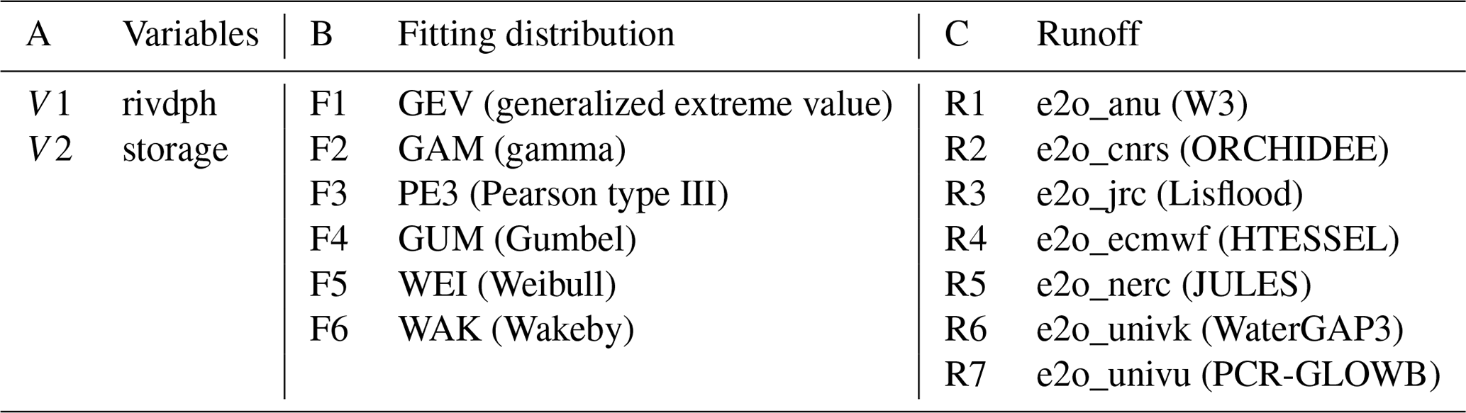
The uncertainty due to the fitting distributions used for FFA was evaluated as the resulting differences by applying various fitting functions (i.e., F1–F6). These distributions are generally used in FFA but for different variables in different fields, and they were treated without priorities in this study. The samples were automatically fitted with L-moments optimization and without any manual modifications in their parameters.

The results of the FFA were based on the output of CaMa-Flood associated with different runoff inputs. In our case, the CaMa-Flood was driven by seven different kinds of runoff forcing (i.e., R1–R7) from eartH2Observe (e2o) category (Schellekens et al., 2017). The runoffs were driven by the same WATCH Forcing Data methodology applied to ERA-Interim data (WFDEI; Weedon et al., 2014) but with different land surface or hydrological models. Therefore, the deviation of the results in the FFA among the seven inputs was the uncertainty caused by the runoff inputs, containing the uncertainties in the rainfall-runoff model processes (model structures and model parameters).

2.2 Global river routing model (CaMa-Flood)

CaMa-Flood is designed to simulate the hydrodynamics in continental-scale rivers. Entire river networks are discretized to irregular unit catchments with the sub-grid topographic parameters of the river channel and floodplains (Fig. 1a). The river discharge and other flow characteristics can be calculated with the local inertial equations along the river network map. The water storage of each unit catchment is the only prognostic variable that is solved with the water balance equation. The water level and flooded area are diagnosed from the water storage at each unit catchment using the sub-grid topographic information (Fig. 1b). Therefore, the estimation of water level will contain additional uncertainties in river bathymetry and topography, while uncertainties in the water storage is dominated by the water flux. Detailed descriptions of the CaMa-Flood can be found in the original papers by Yamazaki et al. (2011, 2012, 2014).

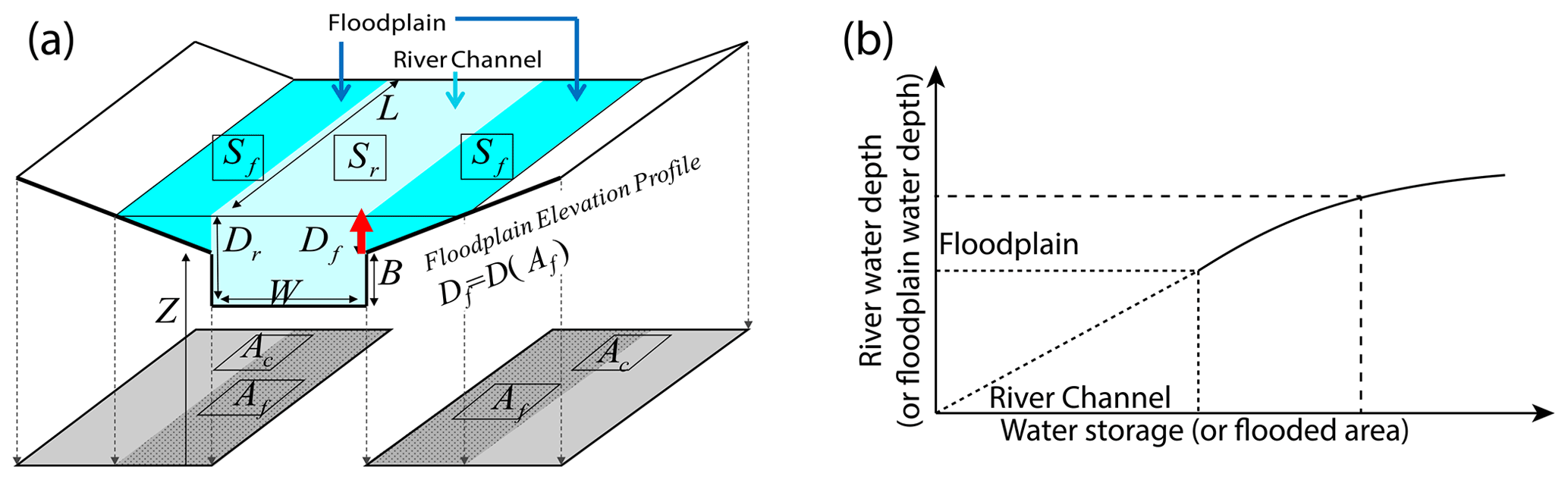
Figure 1 (a) Illustration of a river channel reservoir and a floodplain reservoir defined in each unit catchment. The water level for the river channel and floodplain is assumed to be the same in each unit catchment. The denotation of each parameter and its calculation refer to (Yamazaki et al., 2011). (b) The relationship between the water level and water storage (or flooded area) for a specific unit catchment. The shape of the curve within the river channel is determined by the profile of the river channel, and the curve above the river channel is mainly affected by floodplain topography.

The major advantage of the CaMa-Flood simulations is their explicit representation of flood stage (water level and flooded area) in addition to river discharge. This facilitates the comparison of model results with satellite observations, either the altimeters by synthetic aperture radar (SAR) or inundation images by optical or microwave imagers. The estimation of the flooded area is helpful in the assessment of flood risk and flood damages by overlaying it with socioeconomic datasets.

Another apparent advantage of CaMa-Flood is its high computational efficiency of the global river simulations. CaMa-Flood utilizes a diagnostic scheme at the scale of unit catchment to approximate the complex floodplain inundation processes. The prognostic computation for water storage is optimized by implementing the local inertial equation and the adaptive time step scheme. The high computational efficiency is beneficial for implementations at a global scale. This is critically important because ensemble simulations are frequently applied to account for uncertainties but computation time will be multiplied manyfold. In this study, CaMa-Flood was driven by different runoff inputs (see Sect. 2.1) to achieve the flow characteristics at each unit catchment at the global scale. The FFA is conducted based on the flow characteristics using CaMa-Flood.

2.3 Flood frequency analysis (FFA)

The runoff inputs are available from 1980 to 2014 (35 years in total). For a specific unit catchment defined in the CaMa-Flood, the maximum value of the daily river water depth or catchment water storage was obtained for each year and was then sorted. The frequency as the return period (P_m) was calculated with the following equation:

$$\begin{array}{}\text{(1)}& P_m={\displaystyle \frac{m}{N+\mathrm{1}}},\end{array}$$

where m is the sorted ranking and N denotes the number of total years (herein 35).

The parameters of the fitting distributions were then calculated based on these sorted annual values with the L-moments method (Hosking, 2015; Drissia et al., 2019). This is defined as a linear combination of probability-weighted moments of the time series. The parameter estimations using L-moments and quantile functions used for different distributions have been described in detail in Hosking (1990). The computation of the parameters was done in the Python lmoments3 library. Note that the Wakeby (WAK) is a five-parameter function, the GEV, PE3 and WEI are three-parameter functions, and GAM and GUM are two-parameter functions.

The Akaike information criterion (AIC;  Akaike, 1974) was used to evaluate the performance of the FFA against the annual values. AIC is calculated as

$$\begin{array}{}\text{(2)}& \mathrm{AIC}=\mathrm{2}k+n\cdot \log \left({\displaystyle \frac{\sum (S-O{)}^{\mathrm{2}}}{n}}\right),\end{array}$$

where k is the number of parameters needed for the fitting distribution, S represents the simulated values (here, the fitting values), O represents the observed values (here, the values to be fitted) and n denotes the number of samples. A smaller AIC denotes higher fitting performance because of smaller deviations between simulations and observations. Although there are various performance metrics to measure the goodness of fit, the AIC is used in our study because it will enlarge the tiny difference between samples and estimations. We only have 35 samples and these are sorted, therefore the fitting performance should be very high and the fitting results should not have large differences.

2.4 Downscaling to high-resolution inundation map

To reduce the computation cost due to high-resolution simulations, the CaMa-Flood was run initially at a 0.25^∘ spatial resolution globally, which means that only one unit catchment was assigned for each 25 km by 25 km grid. The performance of the FFA was evaluated with AIC at the global scale to capture the overall features (see Sect. 3.1).

However, it is difficult to characterize the river water depth or inundation area in detail with local topography at such a low resolution (0.25^∘). Meanwhile it is difficult to visualize the inundation map at a high resolution (<100 m) for the globe. Therefore, high-resolution (3 arcsec, ∼90 m at the Equator) regional analysis related to the flood water depth and inundation area with their uncertainties was only conducted regionally over deltas, which are vulnerable to floods (Shin et al., 2020). The corresponding results on the uncertainties in water depth (including at specific points) and inundation area will be presented.

The estimated low-resolution storage was downscaled to the high-resolution inundation map at 90 m with the multi-error-removed improved-terrain (MERIT) DEM topography map (Yamazaki et al., 2017). The fundamental assumption is that the movement of water within a unit catchment is instantaneous and that the water surface is flat within the unit catchment at each time step (Zhou et al., 2020). The total water storage under the identical water level should be equal to the water storage estimated in this unit catchment (see Fig. 1a). The area of lowest elevation is inundated first until the total water volume approximates the estimated water storage of the unit catchment. The relationship between the water level and water storage or the flooded area is illustrated in Fig. 1b. When the floodplain has been inundated, the small increases of water level corresponds to large changes in the water storage and the flooded area. River water depth can be saturated after inundation (it does not react significantly to the increase of storage after flooding) and this might cause an error in function fitting. The assumption of a flat water surface is not valid for large water bodies (e.g., large lakes or reservoirs with water surface gradient) and steep river segments (e.g., mountainous area). However, the impact of violation is limited at the catchment scale with a grid size of 25 km (which is consistent with the global scale). The inundation area over the mountainous area is also limited compared to that in the floodplains.

The flood exposure of the population and economy is estimated based on the inundation map and the 2015 population density map (Gridded Population of the World (GPW)) (CIESIN, 2018) as well as the 2015 Gross Domestic Production map (Kummu et al., 2018). The two maps are in 30 arcsec resolution, therefore the 3 arcsec inundation map was aggregated to the 30 arcsec.

3 Results

3.1 Fitting performance

In this section, we will first analyze the fitting performance using AIC for the different experiments listed in Table 1. Note that the river water depth and the river water storage are in different units or magnitudes. AIC is therefore only applied to the normalized values of water depth or water storage ([0, 1]) for each grid (divided by the maximum value of each grid). The fitting performance was evaluated by the AIC value (Eq. 2). A lower AIC indicates a better fitting performance. Figure 2a and b display a sample result for e2o_ecmwf (R4) and GEV fitting distribution (F1) for water level and storage, respectively. The difference between the two maps is shown in Fig. 2c.

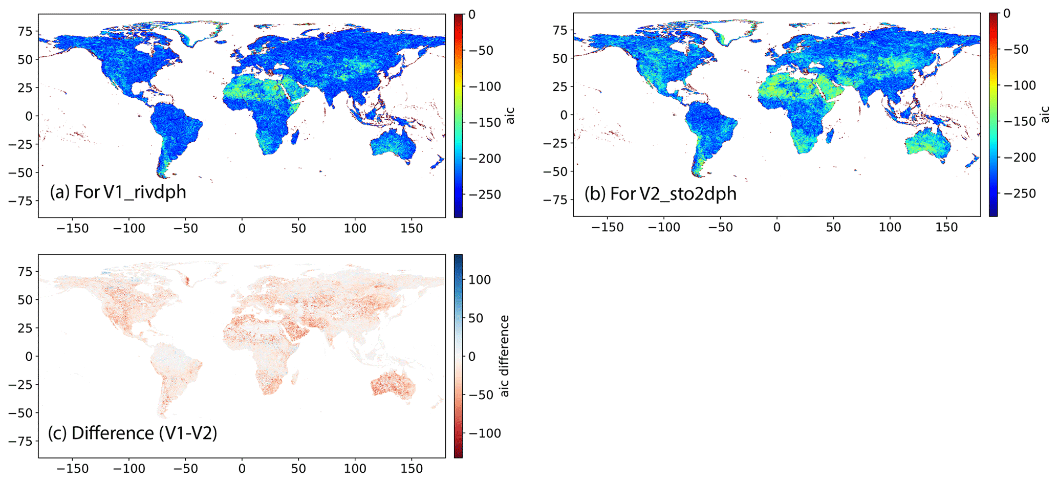
Figure 2 Fitting performance of FFA for (a) V1 (river water depth) and (b) V2 (water storage). The performance was quantified with AIC and (c) is the AIC difference of (a) and (b). This is only an example for the e2o_ecmwf and GEV fitting distribution.

The fitting performance is relatively high with low AIC ($<-\mathrm{50}$) in most of the unit catchments. This happens because we have only a few samples (35) and the time series is normalized to a range between 0 and 1. The advantage of the AIC is that it enlarges the small difference so that we can see a large deviation between different experiments. Relatively low fitting performance is found in the Greenland area and those dry areas in the Sahara, Mongolia and middle Australia (Fig. 2a). The area with low fitting performance (high AIC) increases when dealing with the storage (V2), typically in Mongolia, Australia, South Africa, south Latin America and in the western part of North America. These regions are mainly dominated by dry climate or mountainous topography. The accumulative river discharge over those regions is small and the magnitude is highly dependent on single precipitation events, leading to an unstable relationship between the high floods in different years.

The difference of the AIC values for the river water depth (V1) and that for the storage (V2) is mapped as Fig. 2c. Negative values indicate that the fitting performance is better for water depth than for the water storage. Despite the near-zero values, negative values (red scatters) are distributed in the main parts of the world. The places with the largest differences are distributed in the northern and southern Africa, Australia, northern China and western North America, which are consistent with the high values in Fig. 2b. Although positive values are also found, the values are not large. The results indicate that for most of the lands, the fitting on the data of river water depth is better than the fitting on the water storage. However, this is only the result of a case with e2o_ecmwf runoff input and GEV distribution.

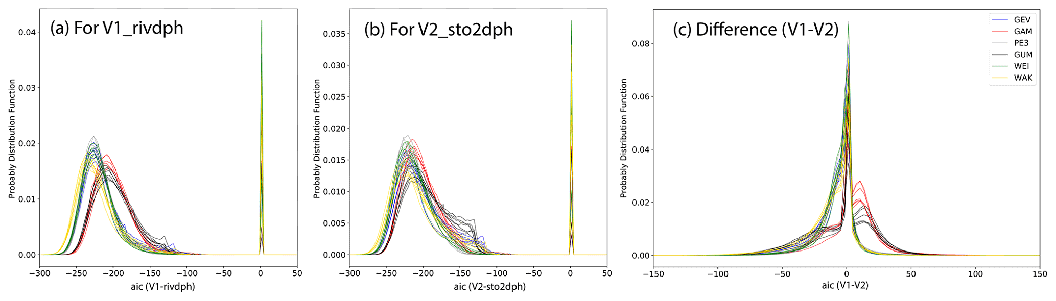
Figure 3 Overall performance of FFA for (a) V1 (river water depth) and (b) V2 (water storage). The performance AIC over all the land grids are collected and displayed as a histogram. Panel (c) is the AIC difference between (a) and (b). Negative difference indicates better performance of FFA for V1. Different colors represent different fitting distributions and the multiple lines in a specific color represents results driven by different runoff inputs. The types of runoff inputs are not specified in these three graphics.

An overall evaluation of all of the distributions and runoff inputs is shown in Fig. 3. The probability distribution of the AIC values for all the global grids are plotted in Fig. 3a and b using water river depth and storage, respectively. The pdf curves have two peaks; one is normally distributed with mean values around −200 (or −220) and the other is near 0. The latter peak around 0 corresponds to the red scatters in Fig. 2a and b, showing poor fitting performance of the distributions over the coastal regions. The difficulties in representing coastal rivers in CaMa-Flood should be the reason or this. From the variations of curves in different curve in the same color, we find that the performance metric AIC is not too sensitive to the runoff. Regarding the differences among different distributions, WAK (yellow lines) has the lowest AIC values with the best performance while GAM (red lines) and GUM (black lines) have the largest values with the poorest performance in Fig. 3a. The other three distributions (GEV, PE3 and WEI) have a similar and moderate performance for water depth. The differences of the fitting performance are mainly due to the degree of freedom of each fitting distribution because the WAK has five parameters, GAM and GUM have two parameters, and the others have three. With a higher degree of freedom, the fitting performance will be better. Meanwhile, compared to fitting with the river water depth, the curves for the water storage were not so distinguishable in Fig. 3b, indicating a lower sensitivity to the fitting distribution. As shown in Fig. 1a, the water level is calculated by allocating the water storage to the river channel and floodplain from the bottom to the top. In the channel, the relationship between water level and storage is linear, while it is nonlinear in the floodplains. So, if the maximum water level for the different years locates in both the river channel and the floodplain, then fitting the water level becomes more difficult, especially for GAM and GUM because they have only two parameters. Given that the storage is not affected by the channel shape, fitting the water storage with different fitting functions will not make a large difference.

Figure 3c shows the difference of fitting performance for water depth and water storage (corresponding to Fig. 2c if e2o_ecmwf and GEV are specified). As in Fig. 2c, negative values indicate that the fitting performance for water depth (V1) is better than that for the water storage (V2). More negative values were found for the distributions of WAK, GEV, PE3 and WEI, especially within the range of [−50, 0]. While for GAM and GUM, more positive values are found within the range of [0, 25], showing better performance for water storage than that for water depth. However, as we see from Fig. 3a and b, the fitting performance of GAM and GUM is not as good as other functions. Because the normalization did not change the ranking of different values, the difference between fitting river water depth and water storage results from their relationship (Fig. 1). For the floods (tails of the fitting distribution), the changes in water storage should be larger than the changes in the water level if the flood frequency shifts. This leads to the resulting difference in the fitting performance. What is limited here is higher fitting performance does not necessarily mean the fitting is appropriate for floods without validation against historical events, which are difficult to access at the global scale. However, measurement of the fitting performance with current available CaMa-Flood estimates is the only way to interpret the variations among different fitting distribution and the small variation of the AIC will be reflected in the extrapolation for flood estimates.

3.2 Flood water depth at a 1-in-100 year return period

3.2.1 Global flood depth

This section summaries the flood water depth and the related uncertainties over the globe at a 1-in-100 year return period (Fig. 4). The results are based on the original estimations of the FFA, rather than the results after normalization presented in the previous section. For the mean values (Fig. 4a), the floodplain water depth will only exceed 10 m in most of the main channels of large rivers, especially in the Amazon River and large rivers in southern China, southeastern Asia and Siberia. The standard deviation of the flood water depth (Fig. 4b) shares the same spatial patterns with the mean values. The deviation in large rivers can reach 5 m or more, which indicates a high degree of uncertainty in estimating the water depth. However, the spatial patterns of the coefficient of variation (C_v, ratio of the standard deviation to the mean) are opposite because C_v is lower where the mean or deviation is higher, and vice versa. The regions with high C_v are likely to be the dry zones (e.g., the Sahara, central Australia and central Asia) and the originating river basins in mountainous regions (e.g., the Rocky Mountains, the Andes and the Tibetan Plateau).

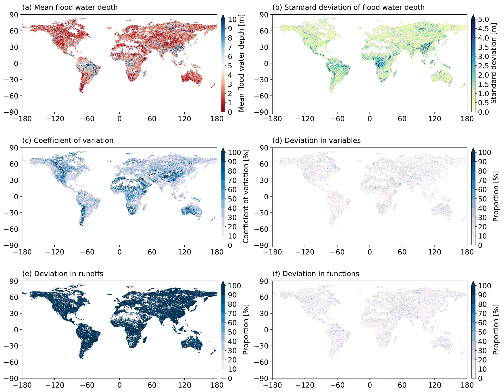
Figure 4 The mean and uncertainties of the flood water depth for the 1-in-100 year flood. The mean flood water depth (a), the standard deviation (b) and the coefficient of variation (c) are estimated based on all of the experiments. The deviation proportion to the overall standard deviation (b) is displayed in (d–f) for different variables, runoffs and fitting functions, respectively.

This deviation in the flood water depth can be caused by various factors, including the used variables, runoffs and the functions listed in Table 1. Figure 4d, e and f show the proportion of the standard deviation due to each factor to the total standard deviation in Fig. 4b. A larger proportion indicates that the deviation due to the corresponding factor contributes more to the total standard deviation. Therefore, for most of the global grids, runoff deviation from different land surface models or global hydrological models is the major contributor, taking a proportion larger than 80 % (Fig. 4e). Schellekens et al. (2017) evaluated the monthly anomalies with the signal-to-noise ratio (SNR) among all runoff inputs that are used in this study. Their results suggested that the runoff has a larger spread over cold regions (e.g., high latitudes in Asia and North America, and the Tibetan Plateau) and dry zones (e.g., the Sahara and central Asia). However, the spatial patterns of runoff spread in their results and the variation in Fig. 4c are not seen in Fig. 4e, indicating that the contribution of runoff to the total uncertainty in flood water depth is not sensitive to climate zones or topography.

The deviation among different variables (Fig. 4d) or functions (Fig. 4f) contributes similarly with a very small proportion to the total deviation. The difference in the deviation due to variables is scatter distributed and likely have larger values in dry regions or coastal areas. While a larger deviation among different fitting functions is primarily found along the large rivers. The difference indicates that the flood water depth will be more sensitive to the functions while less sensitive to selected variables in large rivers (higher water level or larger water storage). Therefore, despite the runoff, more attention is also needed to select the fitting function when evaluating the flood risks for large river basins.

3.2.2 Regional flood water depth

The global analysis is at the spatial resolution of 0.25^∘, which is insufficient to show enough spatial detail. In this section, we evaluate the uncertainty range in the water level and inundation at a much higher spatial resolution (i.e., ∼90 m) after applying the downscaling (see Sect. 2.4). The analysis presented in the main text is for the lower Mekong region where the delta is vulnerable to floods. We also provide results and analyses for other large river basins (e.g., the Amazon, Yangtze, Mississippi, Lena and Nile) in the supporting material (Figs. S1–S5 in the Supplement).

Figure 5a displays the flood water depth for the 1-in-100 year flood at 90 m for the lower Mekong. The largest water depth (>10.0 m) is found in the center of Tonle Sap Lake and the main channel of the Mekong River. A large extent in the lower Mekong delta suffers relatively low inundation water depth (in dark red). Low water depth also occurs along the boundaries of lakes and main channels. The river tributaries have low average water depth in all of the experiments.

Figure 5 The mean and uncertainties of the flood water depth for the 1-in-100 year flood in the lower Mekong River basin. The mean floodplain water depth (a), the standard deviation (b) and the coefficient of variation (c) are estimated based on all the experiments. The deviation proportion to the overall standard deviation (b) is displayed in (d–f) for different variables, runoffs and fitting functions, respectively. The area with floodplain water depth less than 0.01 m are masked out. We use multi-error-removed improved-terrain DEM (MERIT DEM) as the terrain model. The cross in yellow in (a) is the representative GRDC gauge analyzed in the next subsection.

Figure 5b shows the uncertainties resulting from the different experiments listed in Table 1. In general, the uncertainty range is higher where the estimated water depth is deeper (Fig. 5a) because the largest uncertainties are found in the main channel of Mekong River with a magnitude higher than 2.0 m, while the lowest uncertainties are found in the deltas. The uncertainty in the Tonle Sap Lake is homogeneous with a magnitude around 1.0 m. The coefficient of variation (Fig. 5c) is higher where the mean flood water depth and the deviation is smaller. The overall uncertainties mainly result from the runoff inputs (Fig. 5e) and from the fitting distributions (Fig. 5f) and the variables (Fig. 5d). This is consistent with the conclusions from the global analysis.

We also investigated the flood water depth for other rivers, including the Amazon, Yangtze, Mississippi, Lena and Nile (see Figs. S1–S5 in the Supplement) while the conclusions remain similar. Floods will cause a large inundation area in the deltas although the flood water depth is small. Higher uncertainty in water depth with lower coefficient of variation is found in the river channels. While lower uncertainty of water depth with higher coefficient of variation is found for the delta plains. The uncertainties are still mainly caused by the runoff inputs. The selected variables and fitting functions will not lead to large deviations compared to the runoff inputs.

3.3 Flood water depth for multiple return periods

3.3.1 Point analysis

In addition to the global and regional flood pattern at a single return period (1-in-100 year as shown in the previous section), we are also curious to understand how the uncertainty varies at different return periods from 1-in-2 year to 1-in-1000 year. We selected the Phnom Penh GRDC station (Latitude: 11.5617, Longitude: 104.9317, yellow cross in Fig. 5a), which is a representative GRDC gauge at the confluence point of the outlet of the Tonle Sap Lake Lake and the main Mekong River. The estimated mean water depth and the uncertainty range (standard deviation) for different conditions are plotted as the solid line and shaded area, respectively, in Fig. 6. The mean water depth for a 1-in-2 year flood is 8.14 m and 9.58 m for a 1-in-100 year flood (Fig. 6a). The overall standard deviation is large, up to 0.69 m, and it is generally the same for different return periods.

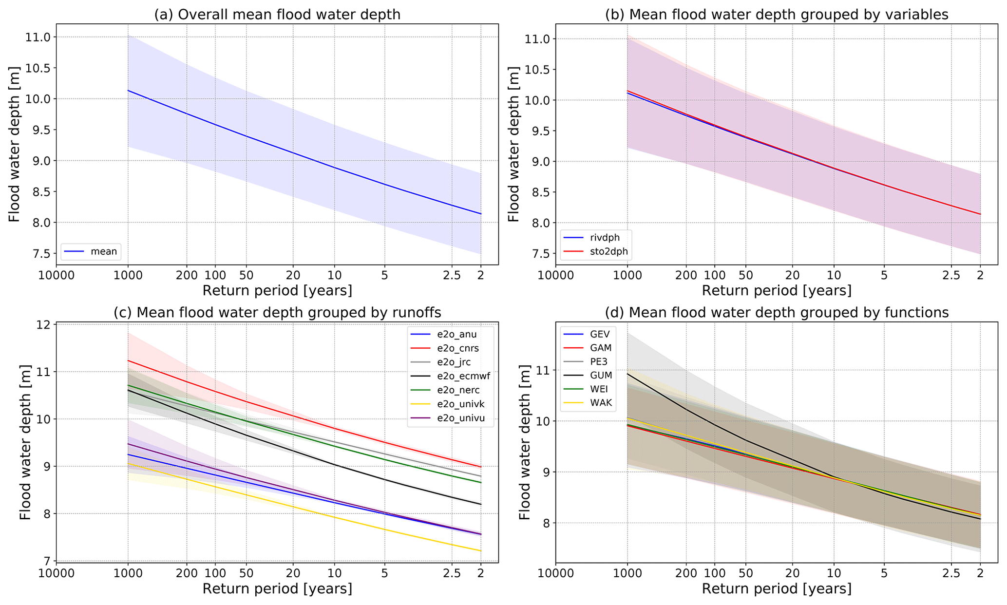
Figure 6 The uncertainties in the estimated flood water depth at Phnom Penh (104.9317^∘ E, 11.5617^∘ N) in the Mekong River basin in different groups. (a) The mean flood water depth and overall uncertainty. (b) The mean and uncertainty in groups of different variables for FFA; the uncertainty is then not related to the selected variable. (c) The mean and uncertainty in groups of different runoff inputs. (d) The mean and uncertainty in groups of different fitting distributions.

In Fig. 6b, the differences between mean flood water depth using river depth (V1) and storage (V2) is very small, while the uncertainty range is still as large as that in Fig. 6a. This indicates that the uncertainty receives little contribution from the variables for FFA. Similarly, subtracting the uncertainty from fitting distributions does not apparently decrease the uncertainty range (Fig. 6d), indicating a small contribution of fitting distributions to the uncertainty. In particular, the mean value for the GUM function in the tails of the floods (more than in the 1-in-20 year flood) is higher than the results of other functions, indicating that GUM may provide a relatively deviated estimate of mean floodplain water depth for the extreme flood events. This difference for GUM mainly happens because GUM only has two degrees of freedom. The uncertainty ranges of other uncertainties except GUM are similar, which indicates that the uncertainty from experiments excluding the fitting distribution is still large.

Figure 6c separates the uncertainties of the runoff inputs from the overall uncertainties. It is notable that the mean values significantly vary from different runoff inputs (solid lines). For the 1-in-100 year flood, the mean water depth ranges from 8.57 m in e2o_univk to 10.58 m in e2o_cnrs (2.01 m in difference). As for each of the runoffs, the uncertainty caused by other sources (variables and fitting distributions; the shaded area in Fig. 6c) is now very small, especially within the normal period covered by the modeled simulations (35 years in this study). Meanwhile, the uncertainty range starts to increase for the extreme floods, as it increases to 0.3–0.5 m for a 1-in-100 year flood (on average 5 % of the total uncertainty) and 0.4–0.6 m for a 1-in-200 year flood, although the uncertainty range is still much smaller than the deviations of the mean values. Similar results are found for other specific points in other river basins and further details can be found in the Supplement.

3.3.2 Inundation area

The uncertainties are also reflected in the inundation area which can be used for assessing the flood exposure of the population or economic losses. Figure 7 displays the results for the lower Mekong River basin at all return periods. The mean values (solid line) and also the uncertainty (standard deviation, colored shades) are displayed in different groups. The mean inundation area increases from 52098 km² for a normal flood (1-in-2 year return period) to 59330 km² corresponding to a 1-in-100 year flood (Fig. 7a).

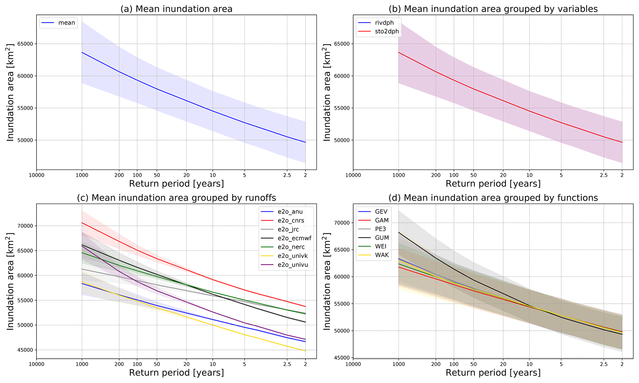
Figure 7 The uncertainties in the estimated inundation area for the study area: (a) shows the mean inundation area and the overall uncertainty; (b–d) show the mean and uncertainty in different groups by variables, runoff inputs and the fitting functions, respectively.

Similar to the features of flood water depth at Phnom Penh (Fig. 6), the magnitude of the uncertainty range in the inundation area is similar for all the return periods (Fig. 7a). The uncertainties also mainly result from the deviation of mean values in different runoff inputs (Fig. 7c) rather than the variables (Fig. 7b) or the fitting functions (Fig. 7d). The predicted inundation area for a 1-in-100 year flood ranges from 54 000 to 64 000 km² in different experiments, indicating a 20 % difference to the largest extent. The standard deviation of the inundation area for a 1-in-100 year flood is around 2000 km², which increases to 3000 km² for a 1-in-200 year flood.

In conclusion, the uncertainties for the inundation area share similar patterns to the results for specific points. These results demonstrate that runoff input is the primary source of uncertainty in river water depth simulation. This uncertainty is mainly due to the systematic bias in the runoff inputs. While for a specific runoff input, the uncertainty is small, especially during the normal period when the estimated values are available (35 years simulation in our case). That extrapolation is applied to FFA in the tails, where the uncertainty range is increased, mainly due to the different tail shape of various fitting distributions. However, the uncertainty range is still smaller than the deviation between results driven by different runoff inputs. Therefore, for impact assessment over the extreme events, the runoff inputs or the average state of the extremes should be evaluated first with observed information, if allowed. Attention can then be given to the selection of different fitting distributions if observations of large floods can be used to optimize the fitting performance, especially in the tails.

3.3.3 Population and economic exposure to floods

Previous results show that the inundation area varies in floods with different return periods in the lower Mekong River basin and many other river basins. This inundation will lead to migration and economic losses, and the impact should be taken with caution because of the uncertainties in inundation estimations. In this section, we evaluate the exposure of the population and economy to the floods at a global scale. The results are summarized for each continent (see Fig. S11 in the Supplement for a location map). The global population density (period per km²) and the economic development (GDP in USD per km²) can be found in Figs. S12 and S13 in the Supplement. Given that runoff is the major source of these uncertainties, we did not show uncertainty ranges due to sources other than the runoff in Fig. 8, although the uncertainty ranges can be found in Fig. S14 in the Supplement.

In total, the inundation area for a 1-in-100 year flood reaches 13×10⁶ km², accounting for 9.1 % of the global area (excluding Antarctica). The ratio for different runoff inputs ranges is 8.1 %–10.3 %. Regarding the population exposure, the gross number is 1.17 billion, accounting for 13.4 % [12.1 %–15 %] of the total population. The potential impact on the GDP will reach up to USD 14.9 trillion on average with a proportion of 13.1 % [11.8 %–14.7 %] of the total values.

Among all continents, Asia will suffer the largest flood extent and also the largest population exposure (above 0.6 million) and economic exposure (above USD 6 trillion) to the floods. Although these values are not the actual flood damages, the potential impact of the flood in Asia (AS) is the highest. The areas with highest population density and economic development is highly consistent with the flood-prone areas (e.g., the Yangtze, Mekong, Ganges and Indus). Compared to AS, North America (NA) will also suffer a large flood extent, while the population and economic exposure is relatively small because the area with high population density or economic development (i.e., the eastern coastal area of the US) is not consistent with the flood-prone area (central plain or Mississippi area). The other continents will suffer smaller inundation area and lower total exposure of the population and economy to the floods. However, it is better to compare the relative values (compared to the specific continent) rather than absolute values because of the area difference.

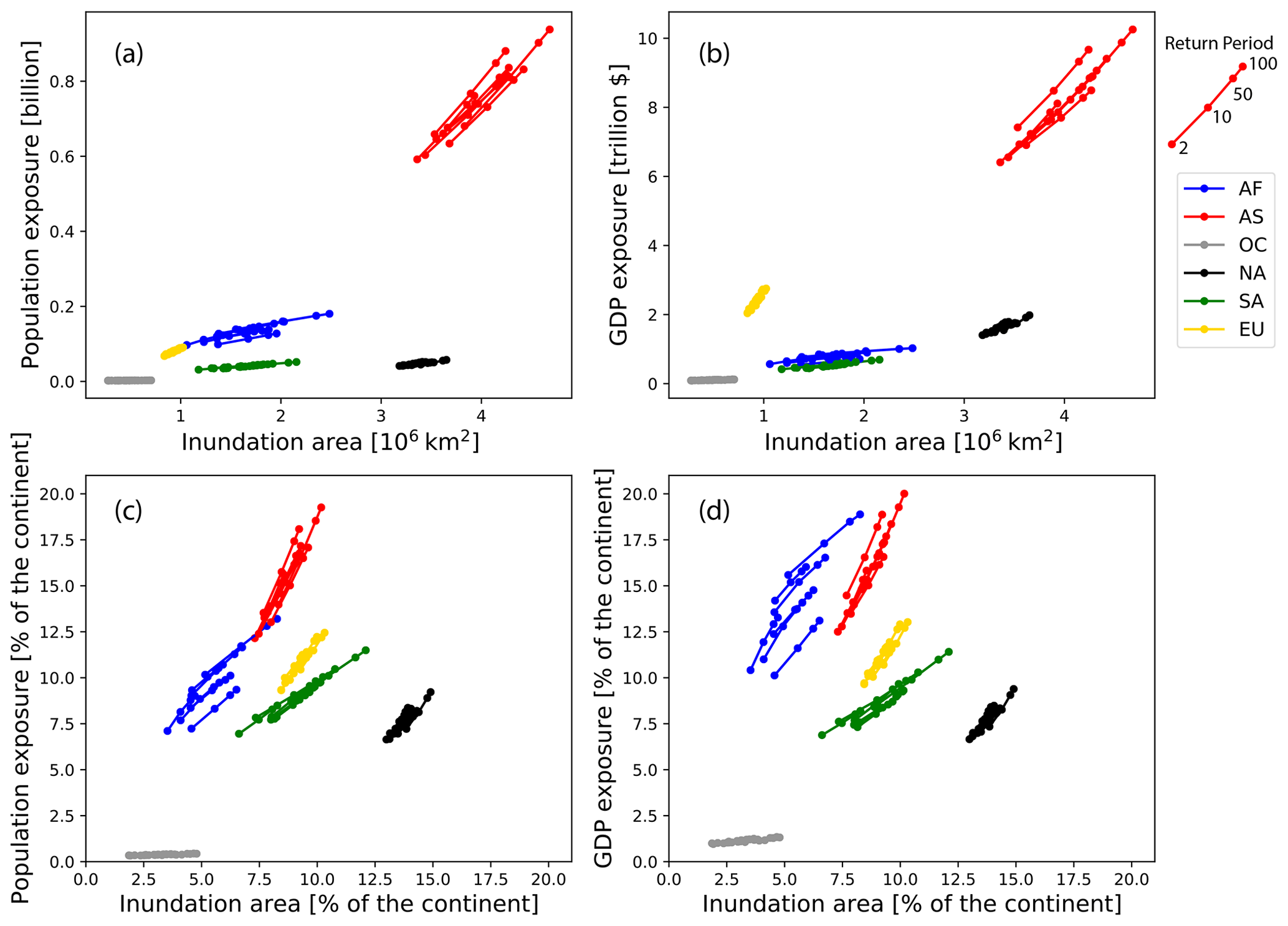
Figure 8 Population and economic exposure to floods in different return periods and the uncertainties due to runoff. The first row shows the absolute values, while the second shows the proportion of total values in the specific continent. The left-hand column shows the population, while the right-hand column shows the gross domestic product. Different colors represent different continents and the values for four different return periods (i.e., 1-in-2, 1-in-10, 1-in-50 and 1-in-100 year) are marked. Different curves in the same color represent the results for various runoff inputs. The names of different runoff inputs are not specified.

Regarding the relative inundation and flood exposure (the second row in Fig. 8), the inundation area accounts for 12.5 %–15 % of the continental area in NA while the flood exposure of population and economy is around 7 %–9 %. In comparison, the inundation area accounts for 3 %–8 % of the continental area in Africa (AF), the population exposure ratio is 7 %–13 % and the economic exposure is 10 %–18 %, indicating a high vulnerability in AF to the floods. The ratio of population exposure in AS (12 %–19 %) is higher than that in AF due to the high consistency of population distribution in southern Asia and the flood-prone areas. The economy in AS (12 %–20 %) is less fragile than that in AF, given a relatively larger flood inundation (7.5 %–10 %). The inundation ratios and flood exposure ratios in other continents are similar, which suggests an even distribution of population and economy in the flood-prone and other regions.

In Fig. 8, the deviations of curves in the same color reflect the uncertainties (Fig. 8d). It is notable that the uncertainties in AF for the economy is the largest. For instance, the highest economic exposure to 1-in-100 year floods approaches 19 % for a certain runoff, while it is 13 % for the lowest with a up to 6 % difference. The economic exposure for a 1-in-2 year flood for the former runoff (>15 %) is already higher than that for the latter 1-in-100 year flood. This deviation is primarily caused by the various processes in the land surface models or hydrological models. However, the parameterization in AF is not well solved among different models compared to other continents, which is probably due to the complexity of the topography and climate zones in AF and data scarcity to calibrate and validate hydrological models. This high degree of uncertainty makes it difficult to accurately assess the economic impact of the floods in the current situation and also for the future projections.

4 Discussions and conclusion

4.1 Discussions

This study assessed the FHM based on simulations with a global hydrodynamic model (CaMa-Flood). The analysis of flood hazards can be uncertain because of the multiple choices of runoff inputs, fitting distributions for the FFA and the variables for the FFA. Our results show that variation in runoff derived from different land surface models and hydrological models is the primary factor behind the uncertainties in flood water depth and the inundation area, as well as the potential flood impact on population and economy.

The FHM and FFA only use the annual maximum water level (or water storage); therefore, the variety only demonstrates the performance of rainfall-runoff models and CaMa-Flood in reproducing the peak discharge. Separation of surface runoff and subsurface runoff, and the evaporation rate during the extreme rain events can lead to the deviations in total runoff and the hydrography after routing. However, in this study, the runoff and the river discharge estimated by CaMa-Flood were not calibrated against observations for each specific runoff because additional calibration will ruin the designed sensitivity test.

There is a lack of studies that have assessed the sensitivities of runoff selection to the flood inundation at a global scale. Although Hirabayashi et al. (2013) assessed the global inundation and population exposure with multiple runoff inputs, their results are simulations for each year rather than for a low-reoccurrence flood. For regions, the estimated inundation area ranges from 3.5 %–9.0 % for a 1-in-100 year flood in Africa (Trigg et al., 2016). It is 4.5 % for the experiment “GloFRIS”, which is the same as our experiment R7 but with different routing DynRout, approximating our results in Africa of 4.4 % [3.5 %–5.2 %]. This suggests that the deviation due to routing models (i.e., DynRout and CaMa-Flood) is limited. However, runoff input is not the direct dominator to the flood but the peak discharge (or peak water level), which is closely associated with the river routing model. Specifically, the topography (Tate et al., 2015), the roughness (Pappenberger et al., 2008; Jung and Merwade, 2012) and spatial resolution of routing (Yu and Lane, 2006; Horritt and Bates, 2001) will slightly change the routing process. The use of different routing methods (namely, linear reservoir, TRIP, travel time routing, Zhao et al., 2017), will lead to larger variations (34 %–85 %) in bias of annual peak discharge for global different GRDC gauges. While using a single routing model (i.e., CaMa-Flood), the bias decreases to 39 %–50 %. However, the sensitivity of the inundation area to routing methods is yet to be investigated and the spatial variation deserves further studies.

With the flood hazard map, the exposure of population and economy to the historical flood can be assessed. This step also has uncertainties as there have been various kinds of products for population and economy. These products are generated with different source data, methods, spatial resolution and time slots (Leyk et al., 2019). Smith et al. (2019) evaluated the population exposure to a 1-in-100 year flood in 18 developing countries. The total exposed population ranges from 101 to 134 million when using three different products, but with an up to 60 % difference in population in Uganda. Changes in the spatial resolution of the population data from 30 to 900 m increases the exposure by 22 %, while decreasing the spatial resolution of flood hazard map from 90 to 900 m increases the exposure by 51 % to 94 % for different products. Therefore, the spatial resolution of the flood hazard map is a particularly important determiner of impact assessment. Validation of the population exposure to real flood events with comparable level should be conducted to decide which spatial resolution is appropriate considering the uncertainties in both the flood estimation and the population products. Such an investigation on the economic impact has not been conducted at a large scale but is required.

One limitation of our study is that we lack validation because the FHMs are not measurable. However, from comparison of long-term water frequency with Landsat and GIEMS data, we noticed that there are some limitations in the current CaMa-Flood that will lead to different results in the uncertainty evaluation. CaMa-Flood does not include flood defense projects (e.g., levees, dams), which will lead to overestimation of the flood inundation in the floodplains and the uncertainty, but lead to underestimation of flood water depth and uncertainties in the river channel. Meanwhile, representing the flood defenses remains a big challenge because the global data for flood defenses are strongly limited (Sampson et al., 2015). Attempts to improve CaMa-Flood by integrating the dam regulation (Shin et al., 2020) and levees (Tanaka and Yamazaki, 2019) have been tested at a regional scale.

5 Conclusions

This study assessed the uncertainties in the FHMs from uncertainty sources, including the variables for FFA, fitting distributions and the runoff inputs, which drive the routing model for estimating the water depth. Among all the uncertainty sources, deviations in runoff inputs contribute the most to the total uncertainty, mainly due to the deviated mean values of extreme water depth. This suggests the importance of rainfall-runoff model calibration (or runoff bias correction) if gauge discharge observation is available. The FHM for the global and specific river basins show the distribution of the mean flood water depth and the uncertainties. Larger deviation values are found in wet regions and along the river channels, while a larger deviation ratio (uncertainty in percentage) is found in dry zones and mountainous regions. Analysis of the flood water depth at specific points and inundation areas for regions displays the uncertainty changes in different return periods. Higher uncertainty is found for a rarer flood compared to normal floods, which is mainly caused by the deviation in the tail shapes of various fitting distributions. Uncertainties in inundation area leads to uncertainties in population and economic exposure to the floods. Globally, 9.1 % of the inundation area for 1-in-100 year floods with 2.2 % uncertainty leads to 13.4 % population exposure (2.9 % uncertainty) and 13.1 % economic exposure (2.9 % uncertainty). The uncertainty is the largest in Africa, which suggests a large deviation in the structures or parameters of hydrological models that are applied in Africa. Overall, model calibration and validation with advanced tools (assimilation of remote sensing products) and also model improvement by taking into account human interventions are needed to reduce the various uncertainties.