the Creative Commons Attribution 4.0 License.
the Creative Commons Attribution 4.0 License.
 | 21 Feb 2020
Back calculation of the 2017 Piz Cengalo–Bondo landslide cascade with r.avaflow: what we can do and what we can learn
Michel Jaboyedoff
José Pullarello
Shiva P. Pudasaini
In the morning of 23 August 2017, around 3×10⁶ m3 of granitoid rock broke off from the eastern face of Piz Cengalo, southeastern Switzerland. The initial rockslide–rockfall entrained 6×10⁵m3 of a glacier and continued as a rock (or rock–ice) avalanche before evolving into a channelized debris flow that reached the village of Bondo at a distance of 6.5 km after a couple of minutes. Subsequent debris flow surges followed in the next hours and days. The event resulted in eight fatalities along its path and severely damaged Bondo. The most likely candidates for the water causing the transformation of the rock avalanche into a long-runout debris flow are the entrained glacier ice and water originating from the debris beneath the rock avalanche. In the present work we try to reconstruct conceptually and numerically the cascade from the initial rockslide–rockfall to the first debris flow surge and thereby consider two scenarios in terms of qualitative conceptual process models: (i) entrainment of most of the glacier ice by the frontal part of the initial rockslide–rockfall and/or injection of water from the basal sediments due to sudden rise in pore pressure, leading to a frontal debris flow, with the rear part largely remaining dry and depositing mid-valley, and (ii) most of the entrained glacier ice remaining beneath or behind the frontal rock avalanche and developing into an avalanching flow of ice and water, part of which overtops and partially entrains the rock avalanche deposit, resulting in a debris flow. Both scenarios can – with some limitations – be numerically reproduced with an enhanced version of the two-phase mass flow model (Pudasaini, 2012) implemented with the simulation software r.avaflow, based on plausible assumptions of the model parameters. However, these simulation results do not allow us to conclude on which of the two scenarios is the more likely one. Future work will be directed towards the application of a three-phase flow model (rock, ice, and fluid) including phase transitions in order to better represent the melting of glacier ice and a more appropriate consideration of deposition of debris flow material along the channel.
- Article
(15676 KB) - Full-text XML
- BibTeX
- EndNote


Landslides lead to substantial damage to life, property, and infrastructure every year. Whereas they have mostly local effects in hilly terrain, landslides in high-mountain areas, with elevation differences of thousands of metres over a few kilometres, may form the initial points of process chains which, due to their interactions with glacier ice, snow, lakes, or basal material, sometimes evolve into long-runout debris avalanches, debris flows, or floods. Such complex landslide events may occur in remote areas, such as the 2012 Alps rock–snow avalanche in Austria (Preh and Sausgruber, 2015) or the 2012 Santa Cruz multi-lake outburst event in Peru (Mergili et al., 2018a). If they reach inhabited areas, such events lead to major destruction even several kilometres away from the source and have led to major disasters in the past, such as the 1949 Khait rock avalanche–loess flow in Tajikistan (Evans et al., 2009b), the 1962 and 1970 Huascarán rockfall–debris avalanche events in Peru (Evans et al., 2009a; Mergili et al., 2018b), the 2002 Kolka–Karmadon ice–rock avalanche in Russia (Huggel et al., 2005), the 2012 Seti River debris flood in Nepal (Bhandari et al., 2012), or the 2017 Piz Cengalo–Bondo rock avalanche–debris flow event in Switzerland. The initial fall or slide sequences of such process chains are commonly related to a changing cryosphere characterized by glacial debuttressing, the formation of hanging glaciers, or a changing permafrost regime (Harris et al., 2009; Krautblatter et al., 2013; Haeberli and Whiteman, 2014; Haeberli et al., 2017).
Computer models assist risk managers in anticipating the impact areas, energies, and travel times of complex mass flows. Conventional single-phase flow models, considering a mixture of solid and fluid components (e.g. Voellmy, 1955; Savage and Hutter, 1989; Iverson, 1997; McDougall and Hungr, 2004; Christen et al., 2010), do not serve such a purpose. Instead, simulations rely on the following:
- i.
model cascades, changing from one approach to the next at each process boundary (Schneider et al., 2014; Somos-Valenzuela et al., 2016) so that each individual model is tailored for the corresponding process component,
- ii.
bulk mixture models or two-phase or even multi-phase flow models (Pitman and Le, 2005; Pudasaini, 2012; Iverson and George, 2014; Mergili et al., 2017; Pudasaini and Mergili, 2019), since two-phase or multi-phase flow models separately consider not only the solid and the fluid phase but also phase interactions and therefore allow for considering more complex process interactions such as the impact of a landslide on a lake or reservoir.
Worni et al. (2014) have highlighted the advantages of the second point for considering also the process interactions and boundaries.
The aim of the present work is to learn about our ability to reproduce sophisticated transformation mechanisms involved in complex, cascading landslide processes with GIS-based tools. For this purpose, we apply the computational tool r.avaflow (Mergili et al., 2017), which employs an enhanced version of the Pudasaini (2012) two-phase flow model, to back calculate the 2017 Piz Cengalo–Bondo landslide cascade in southeastern Switzerland, which was characterized by the transformation of a rock avalanche to a long-runout debris flow. We consider two scenarios in terms of hypothetic qualitative conceptual models of the physical transformation mechanisms. On this basis, we try to numerically reproduce these scenarios, satisfying the requirements of physical plausibility of the model parameters and empirical adequacy in terms of correspondence of the results with the documented and inferred impact areas, volumes, velocities, and travel times. Based on the outcomes, we identify the key challenges to be addressed in future research.
As a result, we rely on the detailed description, documentation, and topographic reconstruction of this recent event. The event documentation, data used, and the conceptual models are outlined in Sect. 2. We briefly introduce the simulation framework r.avaflow (Sect. 3) and explain its parametrization and our simulation strategy (Sect. 4) before presenting (Sect. 5) and discussing (Sect. 6) the results obtained. Finally, we conclude with the key messages of the study (Sect. 7).
2.1 Piz Cengalo and Val Bondasca
Val Bondasca is a left-tributary valley to Val Bregaglia in the canton of Grisons in southeastern Switzerland (Fig. 1). The Bondasca stream joins the Mera River at the village of Bondo at 823 m a.s.l. It drains part of the Bregaglia Range, built up by a mainly granitic intrusive body culminating at 3678 m a.s.l. Piz Cengalo, with a summit elevation of 3368 m a.s.l., is characterized by a steep, intensely fractured northeastern face which has repeatedly been the scene of landslides and which is geomorphologically connected to Val Bondasca through a steep glacier forefield. The glacier itself largely retreated to the cirque beneath the rock wall.
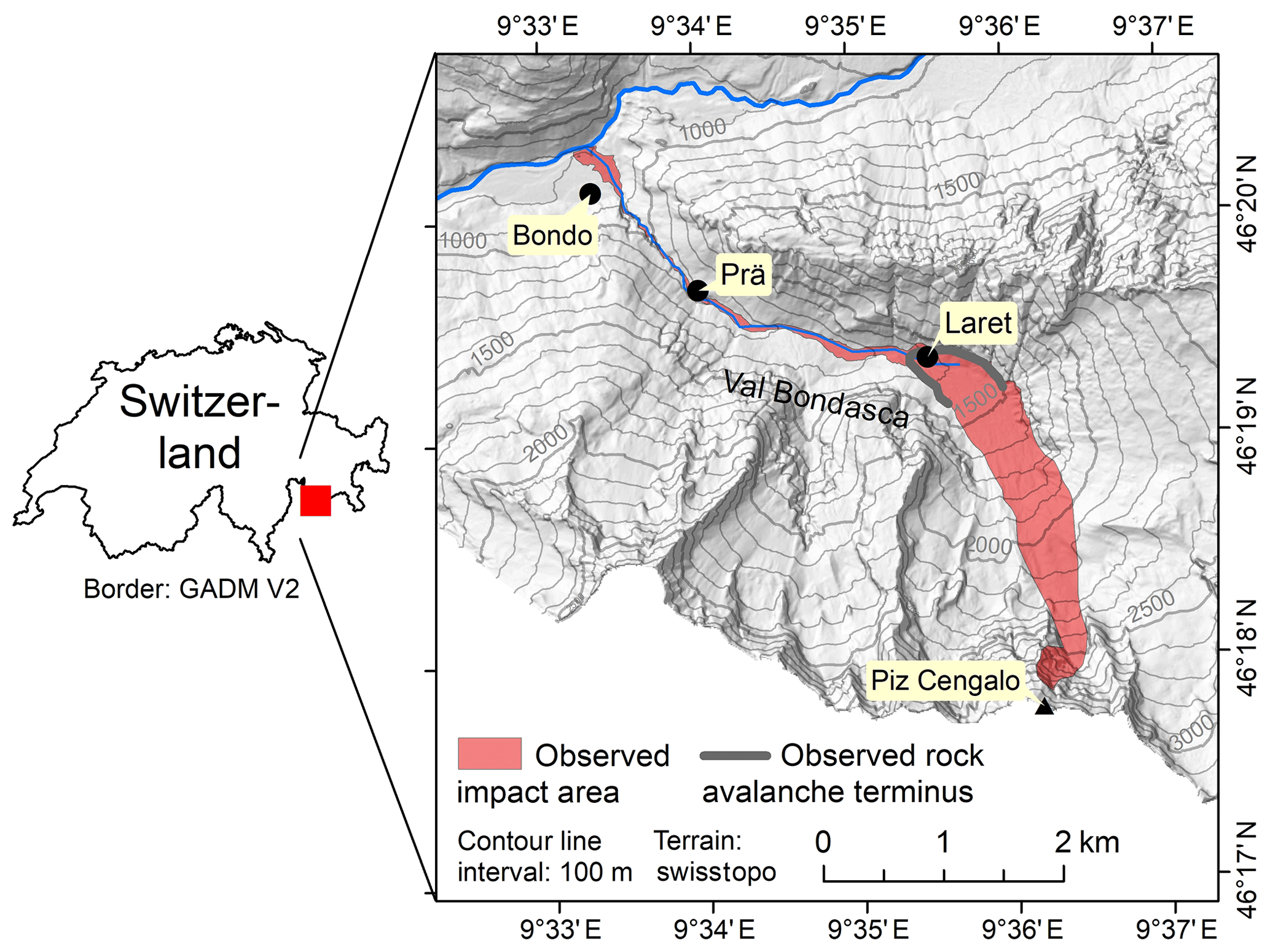
Figure 1Study area with the impact area of the 2017 Piz Cengalo–Bondo landslide cascade. The observed rock avalanche terminus was derived from WSL (2017).
On 27 December 2011, a rock avalanche with a volume of 1.5×10⁶–2×10⁶ m3 developed out of a rock toppling from the northeastern face of Piz Cengalo, travelling for a distance of 1.5 km down to the uppermost part of Val Bondasca (Haeberli, 2013; De Blasio and Crosta, 2016; Amann et al., 2018). This rock avalanche reached the main torrent channel. Erosion of the deposit thereafter resulted in increased debris flow activity (Frank et al., 2019). No entrainment of glacier ice was documented for this event. As blue ice had been observed directly at the scarp, the role of permafrost for the rock instability was discussed. An early warning system was installed and later extended (Steinacher et al., 2018). Displacements at the scarp area, measured by radar interferometry and laser scanning, were a few centimetres per year between 2012 and 2015 and accelerated in the following years. In early August 2017, increased rockfall activity and deformation rates alerted the authorities. A major rockfall event occurred on 21 August 2017 (Amann et al., 2018).
2.2 The event of 23 August 2017
The complex landslide which occurred on 23 August 2017 was documented mainly by reports of the Swiss Federal Institute for Forest, Snow and Landscape Research (WSL); the Laboratory of Hydraulics, Hydrology and Glaciology (VAW) of ETH Zurich; and the Amt für Wald und Naturgefahren (Office for Forest and Natural Hazards) of the canton of Grisons.

Figure 2Oblique view of the impact area of the event from orthophoto draped over the 2011 DTM. Data sources: © swisstopo.
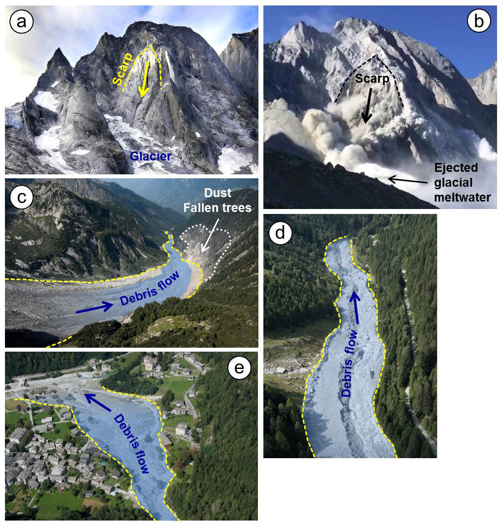
Figure 3The 2017 Piz Cengalo–Bondo landslide cascade. (a) Scarp area on 20 September 2014. (b) Scarp area on 23 September 2017 at 09:30 LT, 20 s after release, in frame of a video taken from the Capanna di Sciora. Note the fountain of water and/or crushed ice at the front of the avalanche, most likely representing meltwater from the impacted glacier. (c) Upper part of Val Bondasca, where the channelized debris flow developed. Note the zone of dust- and pressure-induced damage to trees on the right side of the valley. (d) Traces of the debris flows in Val Bondasca. (e) The debris cone of Bondo after the event. Image sources: © Daniele Porro (a), © Diego Salasc/Reto and Barbara Salis (b), and © swisstopo (c–e).
At 09:31 local time, a volume of approximately 3×10⁶ m3 detached from the northeastern face of Piz Cengalo, as indicated by WSL (2017), Amann et al. (2018), and the point cloud we obtained through structure from motion (SfM) using pictures taken after the event. Documented by videos and by seismic records (Walter et al., 2018), it impacted the glacier beneath the rock face and entrained approximately 6×10⁵ m3 of ice (VAW, 2017; WSL, 2017), was sharply deflected at an opposite rock wall, and evolved into a rock (or rock–ice) avalanche. Part of this avalanche immediately converted into a debris flow which flowed down Val Bondasca. It was detected at 09:34 LT by the debris flow warning system which had been installed near the hamlet of Prä, approximately 1 km upstream from Bondo. According to different sources, the debris flow surge arrived at Bondo between 09:42 (derived from WSL, 2017) and 09:48 LT (Amt für Wald und Naturgefahren, 2017). The rather low velocity in the lower portion of Val Bondasca is most likely a consequence of the narrow gorge topography and of the viscous behaviour of this first surge. Whereas approximately 540 000 m3 of material was involved, only 50 000 m3 arrived at Bondo immediately (data from the canton of Grisons; reported by WSL, 2017). The remaining material was partly remobilized by six further debris flow surges recorded during the same day, one on 25 August, and one – triggered by rainfall – on 31 August 2017. All nine surges together deposited a volume of approximately 500 000–800 000 m3 in the area of Bondo, less than half of which was captured by a retention basin (Bonanomi and Keiser, 2017).
The vertical profile of the main flow path is illustrated in Fig. 4. The total angle of reach of the process chain from the initial release down to the outlet of Val Bondasca was approximately 17.4∘, computed from the travel distance of 7.0 km and the vertical drop of approximately 2.2 km. The initial landslide to the terminus of the rock avalanche showed an angle of reach of approximately 25.8∘, derived from the travel distance of 3.4 km and the vertical drop of 1.7 km. This value is higher than the 22∘ predicted by the equation of Scheidegger (1973), probably due to the sharp deflection of the initial landslide. Following the concept of Nicoletti and Sorriso-Valvo (1991), the rock avalanche was characterized by channelling of the mass. Only a limited run-up was observed, probably due to the gentle horizontal curvature of the valley in that area (no orthogonal impact on the valley slope; Hewitt, 2002). There were eight fatalities, concerning hikers in Val Bondasca, extensive damage to buildings and infrastructure, and evacuations for several weeks or even months.
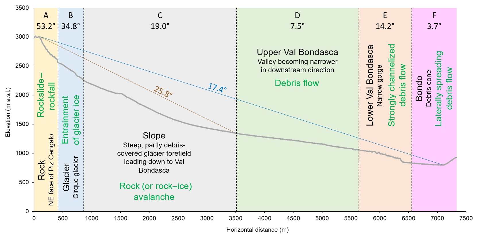
Figure 4Profile along the main flow path of the Piz Cengalo–Bondo landslide cascade. The letters A–F indicate the individual zones (Table 1 and Fig. 7), whereas the associated numbers indicate the average angles of reach along the profile for each zone. The brown number and line show the angle of reach of the initial landslide (rockslide–rockfall and rock – or rock—ice – avalanche), whereas the blue number and line show the angle of reach of the entire landslide cascade. The geomorphic characteristics of the zone (in black) are indicated along with the dominant process type (in green).
2.3 Data and conceptual model
Reconstruction of the rock and glacier volumes involved in the event was based on an overlay of a 2011 swisstopo digital terrain model (DTM; contract: swisstopo–DV084371), derived through airborne laser scanning in 2011 and available at a raster cell size of 2 m, and a digital surface model (DSM) obtained through SfM techniques after the 2017 event. This analysis resulted in a detached rock volume of 3.27×10⁶ m3, which is slightly more than the value of 3.15×10⁶ m3 reported by Amann et al. (2018), and an entrained ice volume of 770 000 m3 (Fig. 5). However, these volumes neglect smaller rockfalls before and after the large 2017 event and also glacial retreat. The 2011 event took place after the DTM had been acquired, but it released from an area above the 2017 scarp. The boundary between the 2011 and the 2017 scarps, however, is slightly uncertain, which explains the discrepancies between the different volume reconstructions. Assuming some minor entrainment of the glacier ice in 2011 and some glacial retreat, we arrive at an entrained ice volume of approximately 600 000 m3, a value which is very well supported by VAW (2017).
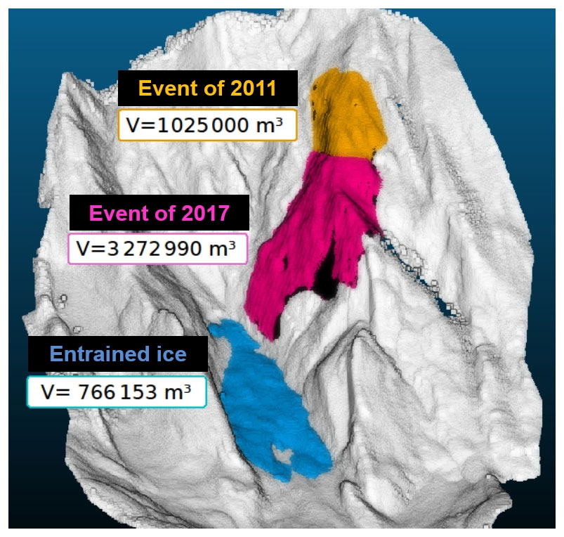
Figure 5Reconstruction of the released rock volume and the entrained glacier volume in the 2017 Piz Cengalo–Bondo landslide cascade. Note that the boundary between the 2011 and 2017 release volumes is connected to some uncertainties, explaining the slight discrepancies among the reported volumes. The glacier volume shown is neither corrected for entrainment related to the 2011 event nor for glacier retreat in the period 2011–2017.
There is still disagreement on the origin of the water that led to the debris flow, particularly to the first surge. Bonanomi and Keiser (2017) clearly mention meltwater from the entrained glacier ice as the main source, whereby much of the melting is assigned to impact, shearing, and frictional heating directly at or after impact, as is often the situation in rock–ice avalanches (Pudasaini and Krautblatter, 2014). WSL (2017) has shown, however, that the energy released was only sufficient to melt approximately half of the glacier ice. Water pockets in the glacier or a stationary water source along the path might have played an important role (Demmel, 2019). Walter et al. (2020) claim that much of the glacier ice was crushed, ejected, and dispersed (Fig. 3b), whereas water injected into the rock avalanche due to pore pressure rise in the basal sediments would have played a major role. In any case, the development of a debris flow from a landslide mass with an overall solid fraction of as high as ∼0.85 (considering the water equivalent of the glacier ice) requires some spatio-temporal differentiation of the water and ice content. We consider two qualitative conceptual models – or scenarios – possibly explaining such a differentiation:
- S1
The initial rockslide–rockfall led to massive entrainment fragmenting, and melting of glacier ice; mixing of rock with some of the entrained ice and the meltwater, and injection of water from the basal sediments into the rock avalanche mass quickly upon impact due to overload-induced pore pressure rise. As a consequence, the front of the rock avalanche was characterized by a high content of ice and water, was highly mobile, and therefore escaped as the first debris flow surge, whereas the less mobile rock avalanche behind it – still with some water and ice in it – decelerated and deposited mid-valley. The secondary debris flow surges occurred mainly due to backwater effects. This scenario largely follows the explanation of Walter et al. (2020) in which the first debris flow surge was triggered at the front of the rock avalanche by overload and pore pressure rise, whereas the later surges overtopped the rock avalanche deposits, as indicated by the surficial scour patterns.
- S2
The initial rockslide–rockfall impacted and entrained the glacier. Most of the entrained ice remained beneath the rock fragments and, after some initial sliding, developed into an avalanching flow of melting ice behind the rock avalanche. The rock avalanche decelerated and stopped mid-valley. Part of the avalanching flow overtopped and partly entrained the rock avalanche deposit – leaving behind the scour traces observed in the field – and evolved into the channelized debris flow which arrived at Bondo a couple of minutes later. The secondary debris flow surges started from the rock avalanche deposit due to melting and infiltration of the remaining ice and due to backwater effects. This scenario is similar to the theory developed at the WSL Institute for Snow and Avalanche Research (SLF), which also did a first simulation of the rock avalanche (WSL, 2017).
Figure 6 illustrates the conceptual models attempting to explain the key mechanisms involved in the rock avalanche–debris flow transformation.
Figure 6Qualitative conceptual models of the rock avalanche–debris flow transformation. (a) Scenario S1. (b) Scenario S2. See text for the detailed description of the two scenarios.
r.avaflow represents a comprehensive GIS-based open-source framework which can be applied for the simulation of various types of geomorphic mass flows. In contrast to most other mass flow simulation tools, r.avaflow utilizes a general two-phase flow model describing the dynamics of the mixture of solid particles and viscous fluid and the strong interactions between these phases. It further considers erosion and entrainment of surface material along the flow path. These features facilitate the simulation of cascading landslide processes such as the 2017 Piz Cengalo–Bondo event. r.avaflow is outlined in full detail by Mergili and Pudasaini (2019). The code, a user manual, and a collection of test datasets are available from Mergili and Pudasaini (2019). Only the aspects directly relevant to the present work are described in this section.
Essentially, the Pudasaini (2012) two-phase flow model is employed for computing the dynamics of mass flows moving from a defined release area (solid and/or fluid heights are assigned to each raster cell) or release hydrograph (at each time step, solid and/or fluid heights are added at a given profile, moving at a given cross-profile velocity) down through a DTM. The spatio-temporal evolution of the flow is approximated through depth-averaged solid and fluid mass and momentum balance equations (Pudasaini, 2012). This system of equations is solved through the total-variation-diminishing (TVD) non-oscillatory central differencing (NOC) scheme introduced by Nessyahu and Tadmor (1990), adapting an approach presented by Tai et al. (2002) and Wang et al. (2004). The characteristics of the simulated flow are governed by a set of flow parameters (some of them are shown in the Tables 1 and 2).
Table 1Descriptions and optimized parameter values for each of the zones A–F (Figs. 4 and 7). The names of the model parameters are given in the text and in Table 2. The values provided in Table 2 are assigned to those parameters not shown. S1 and S2 refer to the corresponding scenarios.

a Note that in all zones and in both of the scenarios, S1 and S2, δ is assumed to scale linearly with the solid fraction. This means that the values given only apply in case of 100 % solid material. b This only applies to the initial landslide, which is assumed completely dry in Scenario S2. Due to the scaling of δ with the solid fraction, a lower basal friction is required to obtain results similar to Scenario S1, where the rock avalanche contains some fluid. The same values of δ as for Scenario S1 are applied for the debris flow in Scenario S2 throughout all zones. c This volume is derived from our own reconstruction (Fig. 5). In contrast, WSL (2017) gives 3.1×10⁶ m3 and Amann et al. (2018) 3.15×10⁶ m3. d In Scenario S2, the glacier is not directly entrained but instead released behind the rock avalanche. In both scenarios, ice is considered to melt immediately on impact and included in the viscous fluid fraction. See text for more detailed explanations.
Table 2Model parameters used for the simulations.
a Fluid is considered here to be a mixture of water and fine particles. This explains the higher density compared to pure water. b The internal friction angle φ always has to be larger than or equal to the basal friction angle δ. Therefore, in the case of δ>φ, φ is increased accordingly.
The solid and fluid phases have their own mass and momentum balance equations so that they evolve as independent dynamical quantities while the phases are still coupled. This means that, in general, the solid and fluid velocities are different. However, the use of an enhanced drag model (Pudasaini, 2019) and the consideration of virtual mass forces ensure a strong coupling between the solid and the fluid phases in the mixture (Pudasaini, 2012; Pudasaini and Mergili, 2019). Compared to the Pudasaini (2012) model, some further extensions have been introduced which include (i) ambient drag or air resistance (Kattel et al., 2016; Mergili et al., 2017) and (ii) fluid friction, governing the influence of basal surface roughness on the fluid momentum (Mergili et al., 2018b). Both extensions rely on empirical coefficients, CAD for the ambient drag and CFF for the fluid friction. Further, viscosity is computed according to an improved concept. As in Domnik et al. (2013) and Pudasaini and Mergili (2019), the fluid viscosity is enhanced by the yield strength. Most importantly, the internal friction angle φ and the basal friction angle δ of the solid are scaled with the solid fraction in order to approximate effects of reduced interaction between the solid particles and the basal surface in fluid-rich flows.
Entrainment is calculated through an empirical model. In contrast to Mergili et al. (2017), where an empirical entrainment coefficient is multiplied by the momentum of the flow, here we multiply the entrainment coefficient CE (s kg−1 m−1) by the kinetic energy of the flow:
where qE,s and qE,f (m s−1) are the solid and fluid entrainment rates, Ts and Tf (J) are the kinetic energies of the solid and fluid fractions of the flow, and αs,E is the solid fraction of the entrainable material. Solid and fluid flow heights and momenta, and the change of the basal topography, are updated at each time step (see Mergili et al., 2017, for details).
As r.avaflow operates on the basis of GIS raster cells, its output essentially consists of raster maps – for all time steps and for the overall maximum – of solid and fluid flow heights, velocities, pressures, kinetic energies, and entrained heights. In addition, output hydrograph profiles may be defined by which solid and fluid heights, velocities, and discharges are provided at each time step.
One set of simulations is performed for each of the scenarios, S1 and S2 (Fig. 6), considering the process chain from the release of the rockslide–rockfall to the arrival of the first debris flow surge at Bondo. Neither triggering of the event nor subsequent surges or distal debris floods beyond Bondo are considered in this study. Equally, the dust cloud associated to the rock avalanche (WSL, 2017) is not the subject here. Initial sliding of the glacier beneath the rock avalanche, as assumed in Scenario S2, cannot directly be modelled. That would require a three-phase model, which is beyond the scope here. Instead, release of the glacier ice and meltwater is assumed in a separate simulation after the rock avalanche has passed over it. We consider this workaround an acceptable approximation of the postulated scenario (Sect. 6).
We use the 2011 swisstopo DTM, corrected for the rockslide–rockfall scarp and the entrained glacier ice by overlay with the 2017 SfM DSM (Sect. 2). The maps of release height and maximum entrainable height are derived from the difference between the 2011 swisstopo DTM and the 2017 SfM DSM (Fig. 5; Sect. 2). The release mass is considered completely solid, whereas the entrained glacier is assumed to contain some solid fraction (coarse till). The glacier ice is assumed to melt immediately on impact and is included in the fluid along with fine till. We note that the fluid phase does not represent pure water but rather a mixture of water and fine particles (Table 2). The fraction of the glacier allowed to be incorporated in the process chain is empirically optimized (Table 3). Based on the same principle, the maximum depth of entrainment of fluid due to pore pressure overload in Scenario S1 is set to 25 cm, whereas the maximum depth of entrainment of the rock avalanche deposit in Scenario S2 is set to 1.5 m.
Table 3Selected output parameters of the simulations for the scenarios S1 and S2 compared to the observed or documented parameter values. S is solid, F is fluid, fractions are expressed in terms of volume, and t0 is time from the initial release to the release of the first debris flow surge. Reference values are extracted from Amt für Wald und Naturgefahren (2017), Bonanomi and Keiser (2017), and WSL (2017). *** is empirically adequate (within the documented range of values). ** is empirically partly adequate (less than 50 % away from the documented range of values). * is empirically inadequate (at least 50 % away from the documented range of values). The arithmetic means of minimum and maximum of each range are used for the calculations.
a Not all the material entrained from the glacier was relevant to the first debris flow surge (Fig. 6); therefore lower volumes of entrained S (coarse till; in Scenario S2 also rock avalanche deposit) and F (molten ice and fine till; in Scenario S1 also pore water) yield the empirically most adequate results. The F volumes originating from the glacier in the simulations represent approximately half of the water equivalent of the entrained ice, corresponding well to the findings of WSL (2017). b This value does not include the 145 000 m3 of solid material remobilized through entrainment from the rock avalanche deposit in Scenario S2. c WSL (2017) states that the rock avalanche came to rest approximately 60 s after release, whereas the seismic signals ceased 90 s after release. d A certain time (here, we assume a maximum of 30 s) has to be allowed for the initial debris flow surge to reach O2, located slightly downstream of the front of the rock avalanche deposit. e WSL (2017) gives a travel time of 3.5 min to Prä, roughly corresponding to the location of O3. It remains unclear whether this number refers to the release of the initial rockslide–rockfall or (more likely) to the start of the first debris flow surge. Bonanomi and Keiser (2017) give a travel time of roughly 4 min between the initial release and the arrival of the first surge at the sensor of Prä. f Amt für Wald und Naturgefahren (2017) gives a time span of 17 min between the release of the initial rockslide–rockfall and the arrival of the first debris flow surge at the “bridge” in Bondo. However, the bridge that this number refers to is not indicated. WSL (2017), in contrast, gives a travel time of 7–8 min from Prä to the “old bridge” in Bondo, which, in sum, results in a shorter total travel time as indicated in Amt für Wald und Naturgefahren (2017). Depending on the bridge, the reference location for these numbers might be downstream from O4. In the simulation, this hydrograph shows a slow onset – travel times refer to the point when 5 % of the total peak discharge is reached.
The study area is divided into six zones, labelled A–F (Figs. 4 and 7; Table 1). Each of these zones represents an area with particular geomorphic characteristics and dominant process types, which can be translated into model parameters. Due to the impossibility of directly measuring the key parameters in the field (Mergili et al., 2018a, b), the parameters summarized in Tables 1 and 2 are the result of an iterative optimization procedure, where multiple simulations with different parameter sets are performed in order to arrive at one “optimum” simulation for each scenario. It is thereby important to note that we largely derive one single set of optimized parameters which is valid for both of the scenarios. Optimization criteria are (i) the empirical adequacy of the model results and (ii) the physical plausibility of the parameters. Therefore, the empirical adequacy is quantified through comparison of the results with the documented impact area; the travel times to the output hydrograph profiles O2, O3, and O4 (Fig. 7); and the reported volumes (Amt für Wald und Naturgefahren, 2017; Bonanomi and Keiser, 2017; WSL, 2017). The physical plausibility of the model parameters is evaluated on the basis on the parameters suggested by Mergili et al. (2017) and on the findings of Mergili et al. (2018a, b). The values of the basal friction angle (δ), the ambient drag coefficient (CAD), the fluid friction coefficient (CFF), and the entrainment coefficient (CE) are differentiated between and within the zones (Table 1), whereas global values are defined for all the other parameters (Table 2). It is further important to note that δ scales linearly with the solid fraction – this means that the values given in Table 1 only apply for 100 % solid material.
Figure 7Overview of the heights and entrainment areas as well as the zonation performed as the basis for the simulation with r.avaflow. Injection of pore water only applies to Scenario A. The zones A–F represent areas with largely homogeneous surface characteristics. The characteristics of the zones and the model parameters associated to each zone are summarized in Table 1 and Fig. 4. O1–O4 represent the output hydrograph profiles. The observed rock avalanche terminus was derived from WSL (2017).
Durations of t=1800 s are considered for both scenarios. At this point in time, the first debris flow surge largely passed and left the area of interest, except for some remaining tail of fluid material. Only heights ≥0.25 m are taken into account for the visualization and evaluation of the simulation results. A threshold of 0.001 m is used for the simulation itself, keeping the loss due to numerical diffusion within a range of <1 %–4 % until the point when the flow first leaves the area of interest. Taking into account the size of the event, a cell size of 10 m is considered the best compromise between capturing a sufficient level of detail and ensuring an adequate computational efficiency and is therefore applied for all simulations.
5.1 Scenario S1 – frontal debris flow surge
Figure 8 illustrates the distribution of the simulated maximum flow heights, maximum entrained heights, and deposition area after t=1800 s, when most of the initial debris flow surge has passed the confluence of the Bondasca stream and the Maira River. The comparison of observed and simulated impact areas results in a critical success index (CSI) of 0.558, a distance to perfect classification (D2PC) of 0.167, and a factor of conservativeness (FoC) of 1.455. These performance indicators are derived from the confusion matrix of true positives, true negatives, false positives, and false negatives. CSI and D2PC measure the correspondence of the observed and simulated impact areas. Both indicators can range between 0 and 1, whereby values of CSI close to 1 and values of D2PC close to 0 point to a good correspondence. FoC indicates whether the observed impact areas are overestimated (FoC > 1) or underestimated by the simulation (FoC < 1). More details are provided by Formetta et al. (2016) and by Mergili et al. (2017, 2018a).
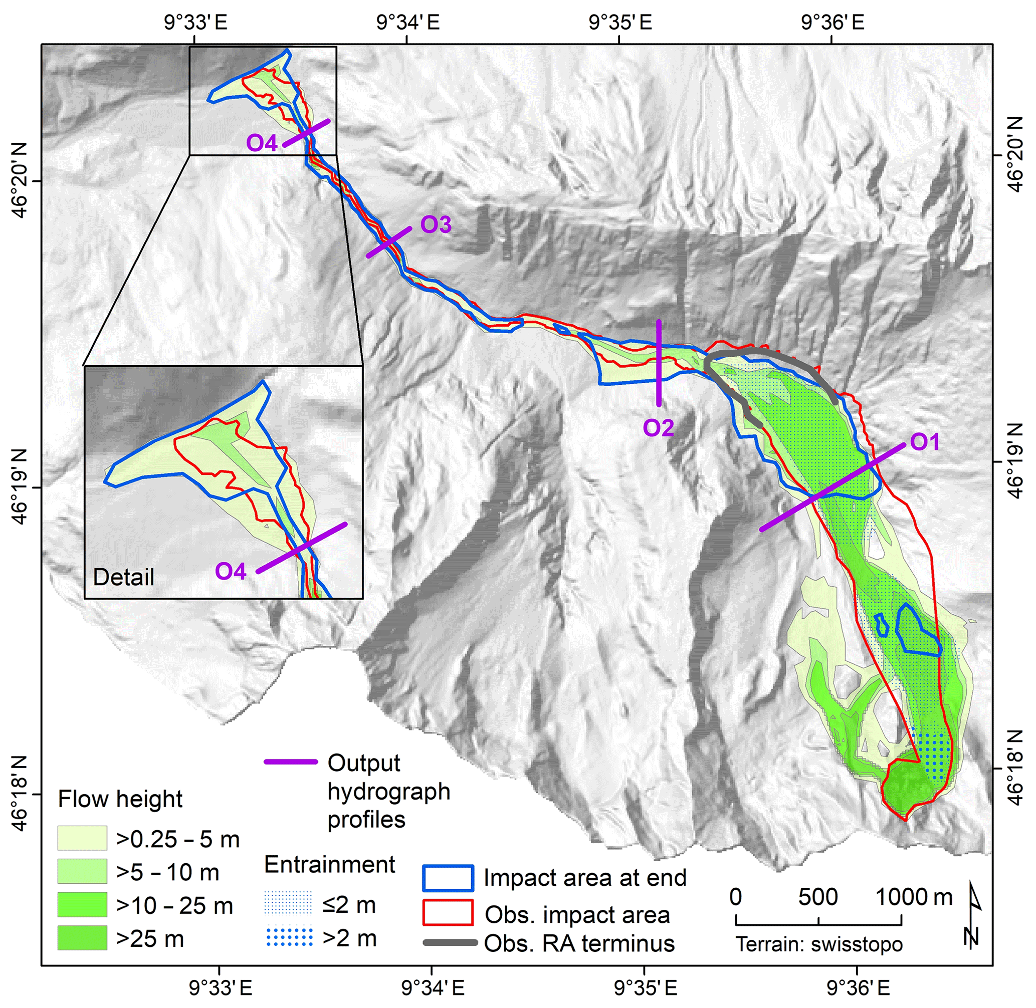
Figure 8Maximum flow height and entrainment derived for Scenario S1. RA is rock avalanche; the observed RA terminus was derived from WSL (2017).
Interpreting these values as indicators for a reasonably good correspondence between simulation and observation in terms of impact area, we now consider the dimension of time, focussing on the output hydrographs OH1–OH4 (Fig. 9; see Figs. 7 and 8 for the location of the corresponding hydrograph profiles O1–O4). Much of the rock avalanche passes the profile O1 between t=60 s and t=100 s. OH2 (Fig. 9a; located in the upper portion of Val Bondasca) sets on before t=140 s and quickly reaches its peak, with a volumetric solid ratio of approximately 30 % (maximum 900 m3 s−1 of solid and 2200 m3 s−1 of fluid discharge). Thereafter, this first surge quickly tails off. The solid flow height, however, increases to around 3 m and remains so until the end of the simulation, whereas the fluid flow height slowly and steadily tails off. Until t=1800 s the profile O2 is passed by a total of 221 000 m3 of solid and 308 000 m3 of fluid material (the fluid representing a mixture of fine mud and water with a density of 1400 kg m−3; see Table 2). The hydrograph profile O3 in Prä, approximately 1 km upstream of Bondo, is characterized by a surge starting before t=280 s and slowly tailing off afterwards. Discharge at the hydrograph OH4 (Fig. 9b; O4 is located at the outlet of the canyon to the debris fan of Bondo) starts at around t=700 and reaches its peak of solid discharge at t=1020 s (167 m3 s−1). Solid discharge decreases thereafter, whereas the flow becomes fluid-dominated with a fluid peak of 202 m3 s−1 at t=1320 s. The maximum total flow height simulated at O4 is 2.53 m. This site is passed by a total of 91 000 m3 of solid and 175 000 m3 of fluid material, according to the simulation – an overestimate, compared to the documentation (Table 3).
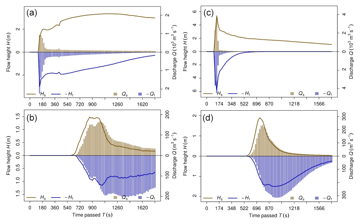
Figure 9Output hydrographs OH2 and OH4 derived for the scenarios S1 and S2. (a) OH2 for Scenario S1. (b) OH4 for Scenario S1. (c) OH2 for Scenario S2. (d) OH4 for Scenario S2. See Figs. 7 and 8 for the locations of the hydrograph profiles O2 and O4. Hs is solid flow height, Hf is fluid flow height, Qs is solid discharge, and Qf is fluid discharge.
Figure 10 illustrates the travel times and the frontal velocities of the rock avalanche and the initial debris flow. The initial surge reaches the hydrograph profile O3 – located 1 km upstream of Bondo – at t=280 s (Fig. 10a; Fig. 9c). This is in line with the documented arrival of the surge at the nearby monitoring station (Table 3). Also the simulated travel time to the profile O4 corresponds to the existing – though uncertain – documentation. The initial rock avalanche is characterized by frontal velocities >25 m s−1, whereas the debris flow largely moves at 10–25 m s−1. Velocities drop below 5 m s−1 in the lower part of the valley (Zone E; Fig. 10b).
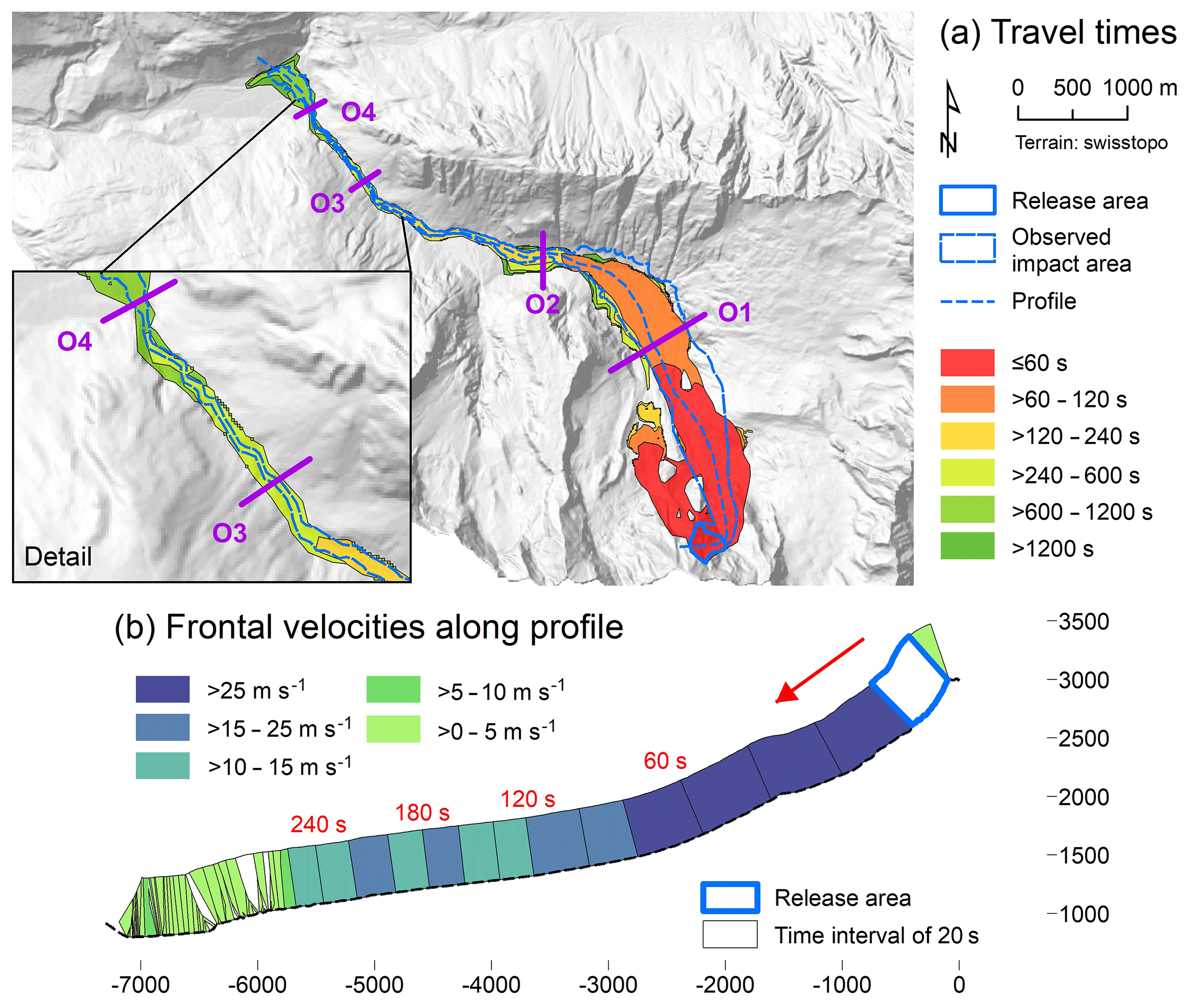
Figure 10Spatio-temporal evolution and velocities of the event obtained for Scenario S1. (a) Travel times, starting from the release of the initial rockslide–rockfall. (b) Frontal velocities along the flow path, shown in steps of 20 s. Note that the height of the velocity graph does not scale with flow height. White areas indicate that there is no clear flow path.
5.2 Scenario S2 – debris flow surge by overtopping and entrainment of rock avalanche
Figure 11 illustrates the distribution of the simulated maximum flow heights, maximum entrained heights, and deposition area after s, where t0 is the time between the release of the initial rock avalanche and the mobilization of the entrained glacier. The simulated impact and deposition areas of the initial rock avalanche are also shown in Fig. 11. However, we now concentrate on the debris flow, triggered by the simulated entrainment of 145 000 m3 of solid material from the rock avalanche deposit. Flow heights – as well as the hydrographs presented in Fig. 9c and d and the temporal patterns illustrated in Fig. 12 – only refer to the debris flow developing from the entrained glacier and the entrained rock avalanche material. The confusion matrix of observed and simulated impact areas reveals partly different patterns of performance than for Scenario S1: CSI = 0.590, D2PC = 0.289, and FoC = 0.925. The lower FoC value and the lower performance in terms of D2PC reflect the missing initial rock avalanche in the simulation results. The output hydrographs OH2 and OH4 differ from the hydrographs obtained through Scenario S1 but also show some similarities (Fig. 9c and d). Most of the flow passes through the hydrograph profile O1 between s and t0+80 s and through O2 between s and t0+180 s. The hydrograph OH2 is characterized by a short peak of 3500 m3 s−1 of solid and 4500 m3 s−1 of fluid material, with a volumetric solid fraction of 0.44, and quickly decreasing discharge afterwards (Fig. 9c). In contrast to Scenario S1, flow heights drop steadily, with values below 2 m from s onwards. The hydrograph OH3 is characterized by a surge starting around s. Discharge at the hydrograph OH4 (Fig. 9d) sets at around s, and the solid peak of 240 m3 s−1 is simulated at approximately s. The delay of the peak of fluid discharge is more pronounced when compared to Scenario S1 (310 m3 s−1 at s). Profile O4 is passed by a total of 65 000 m3 of solid and 204 000 m3 of fluid material. The volumetric solid fraction drops from above 0.60 at the very onset of the hydrograph to around 0.10 (almost pure fluid) at the end. The maximum total flow height at O4 is 3.1 m.
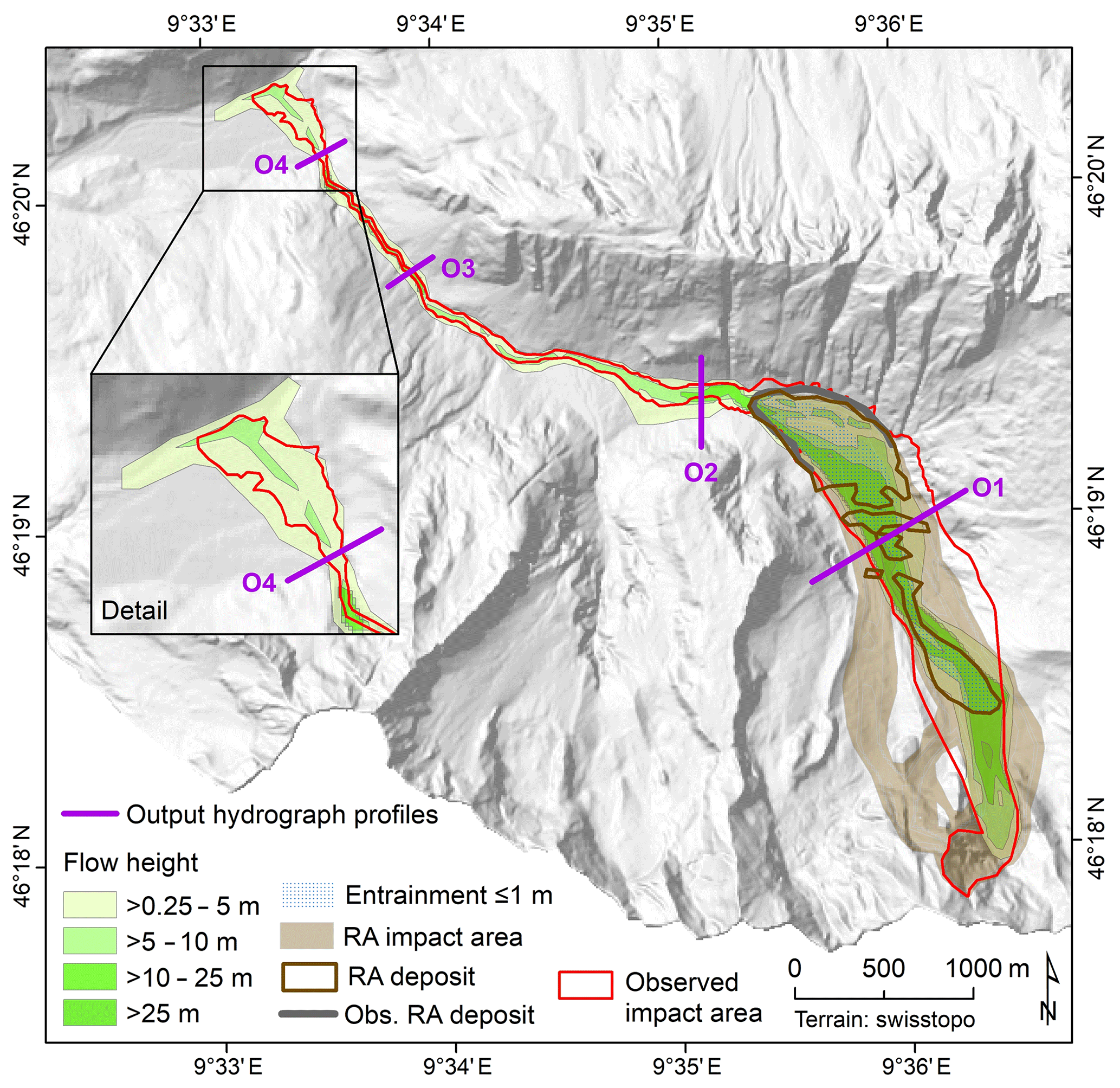
Figure 11Maximum flow height and entrainment derived for Scenario S2. RA is rock avalanche; the observed RA terminus was derived from WSL (2017).
Figure 12 illustrates the travel times and the frontal velocities of the rock avalanche and the initial debris flow. Assuming that t0 is in the range of some tens of seconds, the time of arrival of the surge at O3 is in line with the documentation also for Scenario S2 (Fig. 12a; Table 3). The frontal velocity patterns along Val Bondasca are roughly in line with those derived in Scenario S1 (Fig. 12b). However, the scenarios differ among themselves in terms of the more pronounced but shorter peaks of the hydrographs in Scenario S2 (Fig. 9). This pattern is a consequence of the more sharply defined debris flow surge. In Scenario S1, the front of the rock avalanche deposit constantly releases material into Val Bondasca, providing supply for the debris flow also at later stages. In Scenario S2, entrainment of the rock avalanche deposit occurs relatively quickly, without material supply afterwards. This type of behaviour is strongly coupled to the value of CE and the allowed height of entrainment chosen for the rock avalanche deposit.
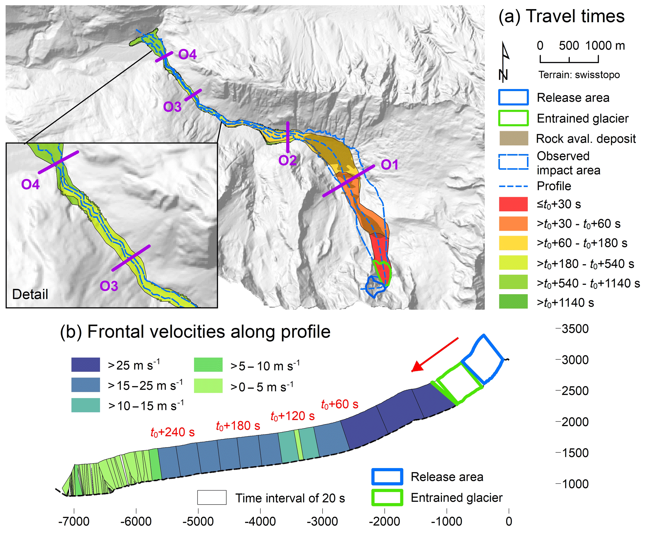
Figure 12Spatio-temporal evolution and velocities of the event obtained for Scenario S2. (a) Travel times, starting from the release of the initial rockslide–rockfall. Therefore t0 (s) is the time between the release of the rockslide–rockfall and the mobilization of the entrained glacier. (b) Frontal velocities along the flow path, shown in steps of 20 s. Note that the height of the velocity graph does not scale with flow height. White areas indicate that there is no clear flow path.
Our simulation results reveal a reasonable degree of empirical adequacy and physical plausibility with regard to most of the reference observations. Having said that, we have also identified some important limitations which are now discussed in more detail. First of all, we are not able to decide on the more realistic of the two scenarios, S1 and S2. In general, the melting and mobilization of glacier ice upon rockslide–rockfall impact are hard to quantify from straightforward calculations of energy transformation, as Huggel et al. (2005) have demonstrated on the example of the 2002 Kolka–Karmadon event. In the present work, the assumed amount of melting (approximately half of the glacier ice) leading to the empirically most adequate results corresponds well to the findings of WSL (2017), indicating a reasonable degree of plausibility. It remains equally difficult to quantify the amount of water injected into the rock avalanche by overload of the sediments and the resulting pore pressure rise (Walter et al., 2020). Confirmation or rejection of conceptual models with regard to the physical mechanisms involved in specific cases would have to be based on better-constrained initial conditions and the availability of robust parameter sets.
We note that with the approach chosen we are not able (i) to adequately simulate the transition from solid to fluid material and (ii) to consider rock and ice separately with different material properties, which would require a three-phase model and is thus not within the scope here. Therefore, entrained ice is considered viscous fluid from the beginning. A physically better-founded representation of the initial phase of the event would require an extension of the flow model employed. Such an extension could build on the rock–ice avalanche model introduced by Pudasaini and Krautblatter (2014). Also, the vertical patterns of the situation illustrated in Fig. 5 cannot be modelled with the present approach, which (i) does not consider melting of ice and (ii) only allows one entrainable layer at each pixel. The assumption of fluid behaviour of entrained glacier ice therefore represents a necessary simplification which is supported by observations (Fig. 3b) but neglects the likely presence of remaining ice in the basal part of the eroded glacier, which melted later and so contributed to the successive debris flow surges.
Still, we currently consider the Pudasaini (2012) model – and the extended multi-phase model (Pudasaini and Mergili, 2019) – to be best practice, even though other two-phase or bulk mixture models do exist. Most recently, Iverson and George (2014) presented an approach that has been solved with an open-source software, called D-Claw (George and Iverson, 2014), and compared it to large-scale experiments considering dense debris materials (Iverson et al., 2000, 2010). The Iverson and George (2014) model can be useful for flow-type landslides, or bulk motion, where the solid particles and fluid molecules move together. However, the Pudasaini (2012) model is better suited for the simulation of cascading mass flows for the following reasons: (i) solid and fluid velocities are considered separately, which is important for complex, cascading mass flows; (ii) pore fluid diffusion is included, whereas the model of Iverson and George (2014) is limited to pore pressure advection and source terms associated with dilation; (iii) interfacial momentum transfers, such as the drag force, virtual mass force, and buoyancy between the solid and fluid phases are fully included; and (iv) viscous shear stress and dynamical coupling between the pore fluid pressure evolution and the bulk momentum equations are considered.
The initial rockslide–rockfall and the rock avalanche are simulated in a plausible way, at least with regard to the deposition area. Whereas the simulated deposition area is clearly defined in Scenario S2, this is to a lesser extent the case in Scenario S1, where the front of the rock avalanche directly transforms into a debris flow. Both scenarios seem to overestimate the time between release and deposition compared to the seismic signals recorded – an issue also reported by WSL (2017) for their simulation. We observe a relatively gradual deceleration of the simulated avalanche, without clearly defined stopping, and note that also in Scenario S2, there is some diffusion after the considered time of 120 s so that the definition of the simulated deposit is somehow arbitrary. The elaboration of well-suited stopping criteria, going beyond the very simple approach introduced by Mergili et al. (2017), remains a task for the future. However, as the rock avalanche has already been successfully back calculated by WSL (2017), we focus on the first debris flow surge: the simulation input is optimized towards the back calculation of the debris flow volumes entering the valley at the hydrograph profile O2 (Table 3). The travel times to the hydrograph profiles O3 and O4 are reproduced in a plausible way in both scenarios, and so are the impact areas (Figs. 8 and 11). Exceedance of the lateral limits in the lower zones is attributed to an overestimate of the debris flow volumes there and to numerical issues related to the narrow gorge: the steep walls of the gorge, in combination with the low number of raster cells representing the width of the flow, challenge the correct geometric representation of the flow in the topography-following coordinate system. Further, application of the TVD NOC scheme results in numerical diffusion which becomes particularly evident in this situation. The introduction of adaptive meshes – which would help to locally increase the spatial resolution while maintaining the computational efficiency – could alleviate this type of issue in the future. The same is true for the fan of Bondo. The solid ratio of the debris flow in the simulations appears realistic, ranging from around 40 % to 45 % in the upper part of the debris flow path and from around 30 % to 35 % and lower (depending on the cut-off time of the hydrograph) in the lower part. This means that solid material tends to stop in the transit area rather than fluid material, as can be expected. Nevertheless, the correct simulation of the deposition of debris flow material along Val Bondasca remains a major challenge (Table 3). Even though a considerable amount of effort was put into reproducing the much lower volumes reported in the vicinity of O4, the simulations result in an overestimate of the volumes passing through this hydrograph profile. This is most likely a consequence of the failure of r.avaflow to adequately reproduce the deposition pattern in the zones D and E. Whereas some material remains there at the end of the simulation, more work is necessary to appropriately understand the mechanisms of deposition in viscous debris flows (Pudasaini and Fischer, 2016). Part of the discrepancy, however, might be explained by the fact that part of the fluid material – which does not only consist of pure water but also consists of a mixture of water and fine mud – left the area of interest in the downstream direction and was therefore not included in the reference measurements. That lower part of the process chain was not subject of the present work.
The simulation results are strongly influenced by the initial conditions and the model parameters. Parameterization of both scenarios is complex and highly uncertain, particularly in terms of optimizing the volumes of entrained till and glacial meltwater and injected pore water. In general, the parameter sets optimized to yield empirically adequate results are physically plausible. Reproducing the travel times to O4 in the present study requires the assumption of a low mobility of the flow in Zone E. This is achieved by increasing the friction (Table 1), accounting for the narrow flow channel, i.e. the interaction of the flow with the channel walls, which is not directly accounted for in r.avaflow. Still, the high values of δ given in Table 1 are not directly applied, as they scale with the solid fraction. This type of weighting has to be further scrutinized. We emphasize that also reasonable parameter sets are not necessarily physically true, as the large number of parameters involved (Tables 1 and 2) create a lot of space for equifinality issues (Beven et al., 1996). The higher values of δ in the lower portion of the channel are based on the assumption that δ of the solid material would somehow depend on the momentum or energy of the flow, which – due to the relatively low velocity – is much less in the zones D and, particularly, E. While this assumption, in our opinion, is justified by fluidization and lubrication effects often observed – or inferred – for very rapid mass flows, it remains hard to consider those effects by a well-justified numerical relationship. Until such a relationship (which definitely remains an important subject of future work) has been proposed, we rely on empirically based zonation of friction parameters.
We have further shown that the classical evaluation of empirical adequacy, by comparing observed and simulated impact areas, is insufficient in the case of complex mass flows: travel times, hydrographs, and volumes involved can provide important insight in addition to the quantitative performance indicators used, for example, in landslide susceptibility modelling (Formetta et al., 2016). Further, the delineation of the observed impact area is uncertain, as the boundary of the event is not clearly defined particularly in Zone C. Also, the other reference data are not exact. Therefore, we allow a broad margin (50 % deviation of the observation) for considering the model outcomes as empirically adequate.
The present work is seen as a further step towards a better understanding of the challenges and the parameterization concerning the integrated simulation of complex mass flows. More case studies are necessary to derive guiding parameter sets facilitating predictive simulations of such events (Mergili et al., 2018a, b). A particular challenge of case studies consists of the parameter optimization procedure: in principle, automated methods do exist (e.g. Fischer et al., 2015). However, they have been developed for optimizing globally defined parameters (which are constant over the entire study area) against runout length and impact area, and such tools do a very good job for exactly this purpose. However, they cannot directly deal with spatially variable parameters, as they are defined in the present work. With some modifications they might even serve that purpose – but the main issue is that optimization should also consider shapes and maximum values of hydrograph discharges or travel times at different places of the path. It would be a huge effort to trim optimization algorithms for this purpose and to make them efficient enough to prevent excessive computational times – we consider this to be an important task for the future which is out of the scope of the present work. Therefore, we have used a stepwise expert-based optimization strategy.
We have back calculated the 2017 Piz Cengalo–Bondo landslide cascade in Switzerland, where an initial rockslide–rockfall of approximately 3×10⁶ m3 entrained a glacier, continued as a rock avalanche, and finally converted into a series of debris flows, reaching the village of Bondo at a total distance of 6.5 km. The water causing the transformation into a debris flow might have originated from entrained glacier ice or from water injected from the debris beneath the rock avalanche. Considering the event from its initiation to the first debris flow surge, we have evaluated not only the possibilities but also the challenges in the simulation of such complex landslide events, employing the two-phase model of the software r.avaflow.
Both of the investigated scenarios, S1 (debris flow developing through injected water at the front of the rock avalanche) and S2 (debris flow developing through melted ice at the back of the rock avalanche, overtopping the deposit), lead to empirically reasonably adequate results when back calculated with r.avaflow using physically plausible model parameters. Based on the simulations performed in the present study, final conclusions on the more likely of the mechanisms sketched in Fig. 6 can therefore not be drawn purely based on the simulations. The observed jet of glacial meltwater (Fig. 3b) points towards Scenario S1. The observed scouring of the rock avalanche deposit, in contrast, rather points towards Scenario S2 but could also be associated to subsequent debris flow surges. Open questions include at least (i) the interaction between the initial rockslide–rockfall and the glacier, (ii) flow transformations in the lower portion of Zone C (Fig. 7), leading to the first debris flow surge, and (iii) the mechanisms of deposition of 90 % of the debris flow material along the flow channel in Val Bondasca. Further research is therefore urgently needed to shed more light on this extraordinary landslide cascade in the Swiss Alps. In addition, improved simulation concepts are required to better capture the dynamics of complex landslides in glacierized environments: this would particularly have to include a three-phase model, where ice – and melting of ice – are considered in a more explicit way. Finally, more case studies of complex mass flows have to be performed in order to derive guiding parameter sets serving for predictive simulations.
The r.avaflow code, including a detailed manual, is available for download at https://www.avaflow.org/ (Mergili and Pudasaini, 2019).
The study is largely based on the 2011 swisstopo digital terrain model (DTM; contract: swisstopo–DV084371) and derivatives thereof. Unfortunately, the authors are not entitled to make these data publicly available.
MM contributed to the conceptualization and methodology of the research; designed the software; and performed the formal analysis, visualization, validation, and most of the writing of the original draft. MJ was involved in the conceptualization, investigation, and supervision as well as in the review and editing of the paper. JP contributed to the investigation, visualization, and review and editing. SPP provided input in terms of methodology and review and editing of the paper.
The authors declare that they have no conflict of interest.
We are grateful to Sophia Demmel and Florian Amann for valuable discussions as well as to Matthias Benedikt for comprehensive technical assistance.
This research has been supported by the Herbette Foundation, the German Research Foundation (DFG; grant nos. PU 386/5-1 and PU 386/3-1), and the Austrian Science Fund (FWF; grant no. I 1600-N30).
This paper was edited by Margreth Keiler and reviewed by Brian McArdell and one anonymous referee.
Amann, F., Kos, A., Phillips, M., and Kenner, R.: The Piz Cengalo Bergsturz and subsequent debris flows, Geophys. Res. Abstr., 20, 14700, 2018.
Amt für Wald und Naturgefahren: Bondo: Chronologie der Ereignisse, 2 pp., available at: https://www.gr.ch/DE/institutionen/verwaltung/bvfd/awn/dokumentenliste_afw/20170828_Chronologie_Bondo_2017_12_13_dt.pdf (last access: 31 May 2019), 2017.
Beven, K.: Equifinality and Uncertainty in Geomorphological Modelling, in: The Scientific Nature of Geomorphology: Proceedings of the 27th Binghamton Symposium in Geomorphology, 27–29 September 1996, John Wiley & Sons, 289–313, 1996.
Bhandary, N. P., Dahal, R. K., and Okamura, M.: Preliminary Understanding of the Seti River Debris-Flood in Pokhara, Nepal, on May 5th, 2012, ISSMGE Bull., 6, 8–18, 2012.
Bonanomi, Y. and Keiser, M.: Bericht zum aktuellen Bergsturz am Piz Cengalo 2017, Bergeller Alpen im Engadin, 19, Geoforum Umhausen, 19–20 Oktober 2017, 55–60, 2017.
Christen, M., Kowalski, J., and Bartelt, P.: RAMMS: Numerical simulation of dense snow avalanches in three-dimensional terrain, Cold Reg. Sci. Technol., 63, 1–14, https://doi.org/10.1016/j.coldregions.2010.04.005, 2010.
De Blasio, F. V. and Crosta, G. B.: Extremely Energetic Rockfalls: Some preliminary estimates, in: Landslides and Engineered Slopes, Experience, Theory and Practice, 759–764, CRC Press, 2016.
Demmel, S.: Water Balance in Val Bondasca, Initial hydrological conditions for debris flows triggered by the 2017 rock avalanche at Pizzo Cengalo, Master Thesis, ETH Zurich, 50 pp., 2019.
Domnik, B., Pudasaini, S. P., Katzenbach, R., and Miller, S. A.: Coupling of full two-dimensional and depth-averaged models for granular flows, J. Non-Newtonian Fluid Mech., 201, 56–68, https://doi.org/10.1016/j.jnnfm.2013.07.005, 2013.
Evans, S. G., Bishop, N.F., Fidel Smoll, L., Valderrama Murillo, P., Delaney, K. B., and Oliver-Smith, A.: A re-examination of the mechanism and human impact of catastrophic mass flows originating on Nevado Huascarán, Cordillera Blanca, Peru in 1962 and 1970, Eng. Geol., 108, 96–118, https://doi.org/10.1016/j.enggeo.2009.06.020, 2009a.
Evans, S. G., Roberts, N. J., Ischuk, A., Delaney, K. B., Morozova, G. S., and Tutubalina, O.: Landslides triggered by the 1949 Khait earthquake, Tajikistan, and associated loss of life, Engin. Geol., 109, 195–212, https://doi.org/10.1016/j.enggeo.2009.08.007, 2009b.
Fischer, J.-T., Kofler, A., Fellin, W., Granig, M., and Kleemayr, K.: Multivariate parameter optimization for computational snow avalanche simulation in 3d terrain, J. Glaciol., 61, 875–888, https://doi.org/10.3189/2015JoG14J168, 2015.
Formetta, G., Capparelli, G., and Versace, P.: Evaluating performance of simplified physically based models for shallow landslide susceptibility, Hydrol. Earth Syst. Sci., 20, 4585–4603, https://doi.org/10.5194/hess-20-4585-2016, 2016.
Frank, F., Huggel, C., McArdell, B. W., and Vieli, A.: Landslides and increased debris-flow activity: a systematic comparison of six catchments in Switzerland, Earth Surf. Proc. Landforms, 44, 699–712, https://doi.org/10.1002/esp.4524, 2019.
George, D. L. and Iverson, R. M.: A depth-averaged debris-flow model that includes the effects of evolving dilatancy. II. Numerical predictions and experimental tests, Proc. Royal Soc. A, 470, 20130820, https://doi.org/10.1098/rspa.2013.0820, 2014.
Haeberli, W.: Mountain permafrost – research frontiers and a special long-term challenge, Cold Reg. Sci. Technol., 96, 71–76, https://doi.org/10.1016/j.coldregions.2013.02.004, 2013.
Haeberli, W. and Whiteman, C. (Eds.): Snow and Ice-related Hazards, Risks and Disasters, Elsevier, https://doi.org/10.1016/B978-0-12-394849-6.00001-9, 2014.
Haeberli, W., Schaub, Y., and Huggel, C.: Increasing risks related to landslides from degrading permafrost into new lakes in de-glaciating mountain ranges, Geomorphology, 293, 405–417, https://doi.org/10.1016/j.geomorph.2016.02.009, 2017.
Harris, C., Arenson, L. U., Christiansen, H. H., Etzelmüller, B., Frauenfelder, R., Gruber, S., Haeberli, W., Hauck., C., Hölzle, M., Humlum, O., Isaksen, K., Kääb, A., Kern-Lütschg, M. A., Lehning, M., Matsuoka, N., Murton, J. B., Nötzli, J., Phillips, M., Ross, N., Seppälä, M., Springman, S. M., and Vonder Mühll, D.: Permafrost and climate in Europe: Monitoring and modelling thermal, geomorphological and geotechnical responses, Earth-Sci. Rev., 92, 117–171, https://doi.org/10.1016/j.earscirev.2008.12.002, 2009.
Hewitt, K.: Styles of rock-avalanche depositional complexes conditioned by very rugged terrain, Karakoram Himalaya, Pakistan, Rev. Eng. Geol., 15, 345–377, 2002.
Huggel, C., Zgraggen-Oswald, S., Haeberli, W., Kääb, A., Polkvoj, A., Galushkin, I., and Evans, S. G.: The 2002 rock/ice avalanche at Kolka/Karmadon, Russian Caucasus: assessment of extraordinary avalanche formation and mobility, and application of QuickBird satellite imagery, Nat. Hazards Earth Syst. Sci., 5, 173–187, https://doi.org/10.5194/nhess-5-173-2005, 2005.
Iverson, R. M.: The physics of debris flows, Rev. Geophys., 35, 245–296, https://doi.org/10.1029/97RG00426, 1997.
Iverson, R. M. and George, D. L.: A depth-averaged debris-flow model that includes the effects of evolving dilatancy. I. Physical basis, Proc. Royal Soc. A, 470, 20130819, https://doi.org/10.1098/rspa.2013.0819, 2014.
Iverson, R. M., Reid, M. E., Iverson, N. R., LaHusen, R. G., Logan, M., Mann, J. E., and Brien, D. L.: Acute sensitivity of landslide rates to initial soil porosity, Science, 290, 513–516, https.doi.org/10.1126/science.290.5491.513, 2000.
Iverson, R. M., Logan, M., LaHusen, R. G., and Berti, M.: The perfect debris flow? aggregated results from 28 large-scale experiments, J. Geophys. Res., 115, 1–29, https://doi.org/10.1029/2009JF001514, 2010.
Kattel. P , Khattri, K. B., Pokhrel, P. R., Kafle, J., Tuladhar, B. M., and Pudasaini, S. P.: Simulating glacial lake outburst floods with a two-phase mass flow model, Ann. Glaciol., 57, 349–358, https://doi.org/10.3189/2016AoG71A039, 2016.
Krautblatter, M., Funk, D., and Günzel, F. K.: Why permafrost rocks become unstable: a rock–ice-mechanical model in time and space, Earth Surf. Process. Landf., 38, 876–887, https://doi.org/10.1002/esp.3374, 2013.
McDougall, S. and Hungr, O.: A Model for the Analysis of Rapid Landslide Motion across Three-Dimensional Terrain, Can. Geotech. J., 41, 1084–1097, https://doi.org/10.1139/t04-052, 2004.
Mergili, M. and Pudasaini, S. P.: r.avaflow – The open source mass flow simulation model, available at: https://www.avaflow.org/, last access: 7 July 2019.
Mergili, M., Fischer, J.-T., Krenn, J., and Pudasaini, S. P.: r.avaflow v1, an advanced open-source computational framework for the propagation and interaction of two-phase mass flows, Geosci. Model Dev., 10, 553–569, https://doi.org/10.5194/gmd-10-553-2017, 2017.
Mergili, M., Emmer, A., Juřicová, A., Cochachin, A., Fischer, J.-T., Huggel, C., and Pudasaini, S. P.: How well can we simulate complex hydro-geomorphic process chains? The 2012 multi-lake outburst flood in the Santa Cruz Valley (Cordillera Blanca, Perú), Earth Surf. Process. Landf., 43, 1373–1389, https://doi.org/10.1002/esp.4318, 2018a.
Mergili, M., Frank, B., Fischer, J.-T., Huggel, C., and Pudasaini, S. P.: Computational experiments on the 1962 and 1970 landslide events at Huascarán (Peru) with r.avaflow: Lessons learned for predictive mass flow simulations, Geomorphology, 322, 15–28, https://doi.org/10.1016/j.geomorph.2018.08.032, 2018b.
Nessyahu, H. and Tadmor, E.: Non-oscillatory central differencing for hyperbolic conservation laws, J. Comput. Phys., 87, 408–463, https://doi.org/10.1016/0021-9991(90)90260-8, 1990.
Nicoletti, G. P. and Sorriso-Valvo, M.: Geomorphic controls of the shape and mobility of rock avalanches, GSA Bull., 103, 1365–1373, https://doi.org/10.1130/0016-7606(1991)103<1365:GCOTSA>2.3.CO;2, 1991.
Pitman, E. B. and Le, L.: A two-fluid model for avalanche and debris flows, Philos. T. Roy. Soc. A, 363, 1573–1601, https://doi.org/10.1098/rsta.2005.1596, 2005.
Pudasaini, S. P.: A general two-phase debris flow model, J. Geophys. Res.-Earth Surf., 117, F03010, https://doi.org/10.1029/2011JF002186, 2012.
Pudasaini, S. P.: A full description of generalized drag in mixture mass flows, Eng. Geol., 265, 105429, https://doi.org/10.1016/j.enggeo.2019.105429, 2019.
Pudasaini, S. P. and Fischer, J.-T.: A mechanical erosion model for two-phase mass flows, https://arxiv.org/abs/1610.01806, 2016.
Pudasaini, S. P. and Krautblatter, M.: A two-phase mechanical model for rock-ice avalanches, J. Geophys. Res.-Earth Surf., 119, 2272–2290, https://doi.org/10.1002/2014JF003183, 2014.
Pudasaini, S. P. and Mergili, M.: A Multi-Phase Mass Flow Model, J. Geophys. Res.-Earth Surf., 124, 2920–2942, https://doi.org/10.1029/2019JF005204, 2019.
Preh, A. and Sausgruber, J. T.: The Extraordinary Rock-Snow Avalanche of Alpl, Tyrol, Austria. Is it Possible to Predict the Runout by Means of Single-phase Voellmy- or Coulomb-Type Models?, in: Engineering Geology for Society and Territory–Volume 2, edited by: Lollino, G., Giordan, D., Crosta, G. B., Corominas, J., Azzam, R., Wasowski, J., and Sciarra, N., Springer, Cham, https://doi.org/10.1007/978-3-319-09057-3_338, 2015.
Savage, S. B. and Hutter, K.: The motion of a finite mass of granular material down a rough incline, J. Fluid Mech., 199, 177–215, https://doi.org/10.1017/S0022112089000340, 1989.
Scheidegger, A. E.: On the Prediction of the Reach and Velocity of Catastrophic Landslides, Rock Mech., 5, 231–236, https://doi.org/10.1007/BF01301796, 1973.
Schneider, D., Huggel, C., Cochachin, A., Guillén, S., and García, J.: Mapping hazards from glacier lake outburst floods based on modelling of process cascades at Lake 513, Carhuaz, Peru, Adv. Geosci., 35, 145–155, https://doi.org/10.5194/adgeo-35-145-2014, 2014.
Somos-Valenzuela, M. A., Chisolm, R. E., Rivas, D. S., Portocarrero, C., and McKinney, D. C.: Modeling a glacial lake outburst flood process chain: the case of Lake Palcacocha and Huaraz, Peru, Hydrol. Earth Syst. Sci., 20, 2519–2543, https://doi.org/10.5194/hess-20-2519-2016, 2016.
Steinacher, R., Kuster, C., Buchli, C., and Meier, L.: The Pizzo Cengalo and Val Bondasca events: From early warnings to immediate alarms, Geophys. Res. Abstr. 20, 17536, 2018.
Tai, Y. C., Noelle, S., Gray, J. M. N. T., and Hutter, K.: Shock-capturing and front-tracking methods for granular avalanches, J. Comput. Phys., 175, 269–301, https://doi.org/10.1006/jcph.2001.6946, 2002.
VAW: Vadrec dal Cengal Ost: Veränderungen in Vergangenheit und Zukunft, Laboratory of Hydraulics, Hydrology and Glaciology of the Swiss Federal Institute of Technology Zurich, 17 pp., available at: https://www.gr.ch/DE/institutionen/verwaltung/bvfd/awn/dokumentenliste_afw/Cengalo Gletscherentwicklung ETH_2nov_final.pdf (last access: 31 May 2019), 2017.
Voellmy, A.: Über die Zerstörungskraft von Lawinen, Schweizerische Bauzeitung, 73, 159–162, 212–217, 246–249, 280–285, 1955.
Walter, F., Wenner, M., and Amann, F.: Seismic Analysis of the August 2017 Landslide on Piz Cengalo (Switzerland), Geophys. Res. Abstr., 20, 3163-1, 2018.
Walter, F., Amann, F., Kos, A., Kenner, R., Phillips, M., de Preux, A., Huss, M., Tognacca, C., Clinton, J., Diehl, T., and Bonanomi, Y.: Direct observations of a three million cubic meter rock-slope collapse with almost immediate initiation of ensuing debris flows, Earth Planet. Sc. Lett., 351, 106933, https://doi.org/10.1016/j.geomorph.2019.106933, 2020.
Wang, Y., Hutter, K., and Pudasaini, S. P.: The Savage-Hutter theory: A system of partial differential equations for avalanche flows of snow, debris, and mud, ZAMM – J. Appl. Math. Mech., 84, 507–527, https://doi.org/10.1002/zamm.200310123, 2004.
Worni, R., Huggel, C., Clague, J. J., Schaub, Y., and Stoffel, M.: Coupling glacial lake impact, dam breach, and flood processes: A modeling perspective, Geomorphology, 224, 161–176, https://doi.org/10.1016/j.geomorph.2014.06.031, 2014.
WSL: SLF Gutachten G2017.20: Modellierung des Cengalo Bergsturzes mit verschiedenen Rahmenbedingungen, Bondo, GR. WSL-Institut für Schnee- und Lawinenforschung SLF, 69 pp., available at: https://www.gr.ch/DE/institutionen/verwaltung/bvfd/awn/dokumentenliste_afw/SLF_G2017_20_Modellierung_Cengalo_Bergsturz_030418_A.pdf (last access: 31 May 2019), 2017.
- Abstract
- Introduction
- The 2017 Piz Cengalo–Bondo landslide cascade
- The simulation framework r.avaflow
- Parameterization of r.avaflow
- Simulation results
- Discussion
- Conclusions
- Code and data availability
- Author contributions
- Competing interests
- Acknowledgements
- Financial support
- Review statement
- References