the Creative Commons Attribution 4.0 License.
the Creative Commons Attribution 4.0 License.
 | 23 Dec 2020
Wave height return periods from combined measurement–model data: a Baltic Sea case study
Jan-Victor Björkqvist
Sander Rikka
Victor Alari
Aarne Männik
Laura Tuomi
Heidi Pettersson
This paper presents how to account for the lack of sampling variability in model data when they are combined with wave measurements. We addressed the dissimilarities between the types of data by either (i) low-pass filtering the observations or (ii) adding synthetic sampling variability to the model. Measurement–model times series combined with these methods served as the basis for return period estimates of a high wave event in January 2019. During this storm northerly wind speeds in the Baltic Sea rose to 32.5 m s−1 and an unprecedented significant wave height of 8.1 m was recorded in the Bothnian Sea sub-basin. Both methods successfully consolidated the combined time series but produced slightly different results: using low-pass-filtered observations gave lower estimates for the return period than using model data with added sampling variability. Extremes in both types of data followed the same type of theoretical distributions, and our best estimate for the return period was 104 years (95 % confidence 39–323 years). A similar wave event can potentially be more likely in the future climate, and this aspect was discussed qualitatively.
- Article
(5342 KB) - Full-text XML
-
Supplement
(1187 KB) - BibTeX
- EndNote


We have two fundamental ways to get wave information. Models cover large areas, recreate past events, and quantify impacts of future changes in forcing. Their major weakness is that they are not necessarily accurate enough for rare events, such as storms (Cavaleri, 2009). Measurements, again, can provide a certain ground truth that is unmatched even by the best of models. But point measurements cannot confidently represent large areas – neither can they be made in the past or in the future. For certain purposes remote sensing products combine the versatility of (numerical) models and the reliability of (in situ) observations (e.g. Young et al., 2011; Salcedo-Castro et al., 2018). Often, however, models and measurements are used in combination; typically a model is validated and calibrated with observations (e.g. Bidlot et al., 2002; Haiden et al., 2018) before being used to extend limited measurements in time or space (e.g. Caires et al., 2006; Soomere et al., 2008; Breivik et al., 2013).
A lot, then, hinges on whether instruments properly capture physical phenomena despite being limited by unavoidable sampling variability (Longuet-Higgins, 1952; Bitner-Gregersen and Magnusson, 2014). This uncertainty can be around 10 % in significant wave heights measured by wave buoys (Donelan and Pierson, 1983), and Forristall et al. (1996) determined it to lead to a 3 %–7 % bias when estimating 100-year wave heights. Also, wave modellers have noted that their simulated extremes represent a mean over a few hours – not a single 20–30 min measurement (Bidlot et al., 2002; Aarnes et al., 2012; Breivik et al., 2013).
The statistical behaviour of extremes is also unknown. Extreme value analysis has a solid – but wide – theoretical framework (e.g. Coles, 2001), leaving researchers to determine how to define extremes (e.g. Méndez et al., 2006; Orimolade et al., 2016) and with what distribution to model them (e.g. Aarnes et al., 2012; Haakenstad et al., 2020). In addition, there is a globally uneven trend in significant wave heights (Hemer et al., 2013), with the decreasing ice cover being a dominant factor in high latitudes (Stopa et al., 2016; Groll et al., 2017). All the aforementioned issues obscure estimates of how often to expect extreme wave events during, for example, the next decade.
This study examines how to best combine measured and modelled data and how well this merged data set is suited to analyse extremes. The specific focus is a record wave event that took place on 1 January 2019 in the seasonally ice-covered Baltic Sea. There exist no wave buoy data from the study location prior to 2011, but the observations were complemented by hindcasts covering 1965–2013 (Björkqvist et al., 2018; Tuomi et al., 2019). We consolidated the data to a continuous time series using two methods, both of which can be used universally. The return period of the wave event was then inferred from theoretical distributions that were fitted to the combined measurement–model data.
The paper has the following structure. Observations and model data are described in Sect. 2, while methods for combining data and fitting distributions are presented in Sect. 3. An overview of the storm is provided in Sect. 4, before estimating the return period of the wave event in Sect. 5. We discuss our results with respect to the current climate and a future declining ice cover, and we end by concluding our findings.
2.1 Wave buoy observations
Wave buoy data in the Bothnian Sea were available from two sites. The Finnish Meteorological Institute (FMI) has moored a wave buoy in the eastern part of the Bothnian Sea (61∘ 48′ N, 20∘ 14′ E, Fig. 1) at a depth of 120 m. The data cover 79 % of the time 2011–2019, which is a high coverage considering that the wave buoy cannot measure during the ice season. The wave buoy at Finngrundet (60∘ 54′ N, 18∘ 37′ E, Fig. 1) in the southwestern part of the Bothnian Sea is operated by the Swedish Meteorological and Hydrological Institute (SMHI). This buoy is moored at a depth of roughly 70 m about 10 km southeast of an underwater bank. Both wave buoys are Datawell Directional Waveriders. At the Bothnian Sea wave parameters were derived from the wave spectra available every 30 min on the buoy's memory card. The Finngrundet data for the storm duration were extracted from SMHI's open data portal (parameters available every hour).
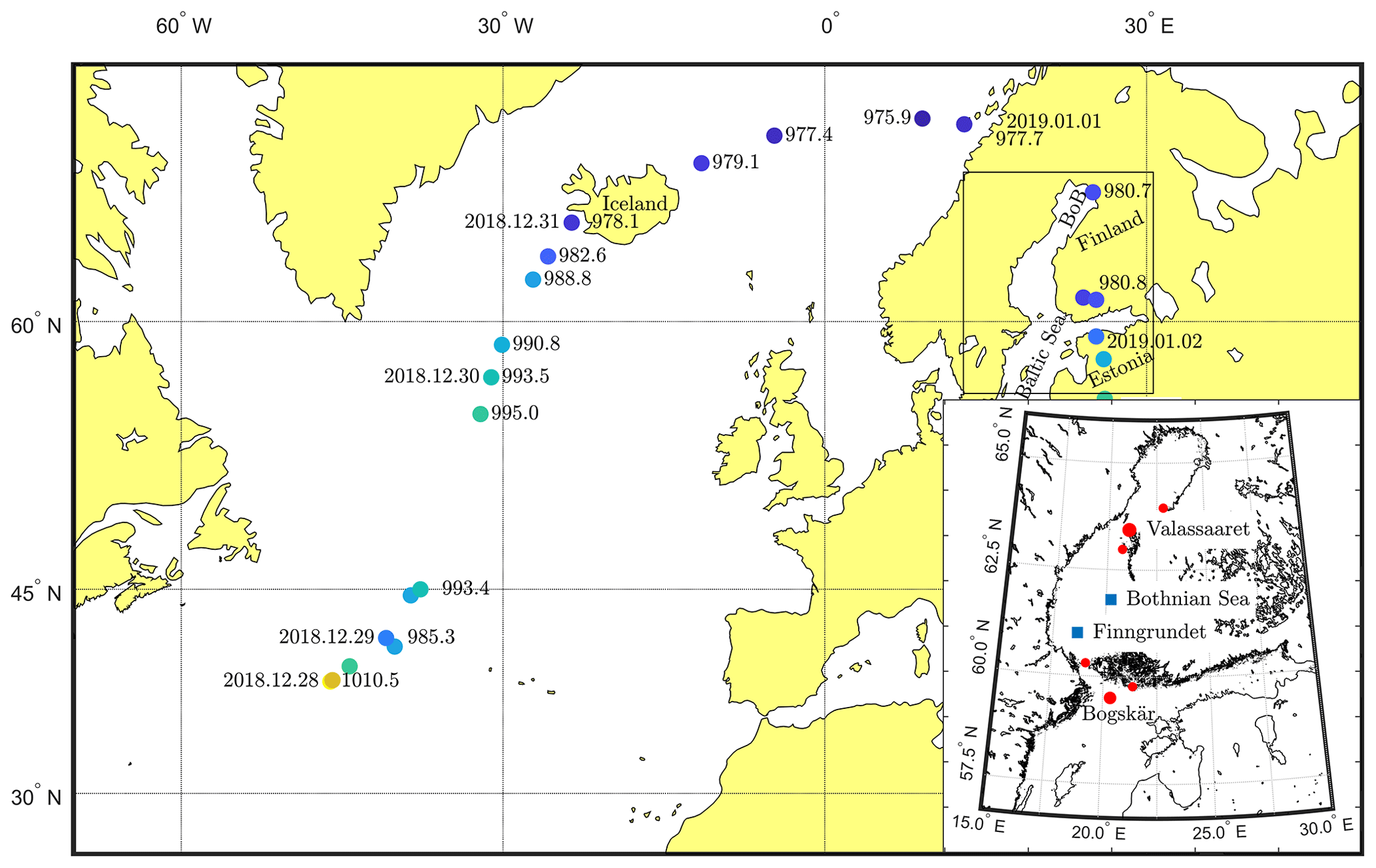
Figure 1Storm track and sea level pressures (hPa) in the centre of the cyclone. The inset shows the Baltic Sea, the location of the wave buoys, and the two main weather stations. The four smaller red circles mark four additional weather stations (from north to south): Tankar, Stömmingbådan, Märket, and Utö.
The significant wave height was determined as , where m0 is the integral of the wave spectrum. The peak period, Tp, was determined as the argument maximum of the spectrum, and the directional parameters of mean direction at the spectral peak, θp, and the directional spreading was determined following e.g. Kuik et al. (1988).
2.2 Wave model data
Two existing Baltic Sea wave hindcasts complemented the Bothnian Sea wave buoy observations. The hindcast of Björkqvist et al. (2018) covered 1965–2005; the data originate from the wave model SWAN (Simulating WAves Nearshore; Booij et al., 1999) that was forced with the 6 h resolution BaltAn65+ wind product (Luhamaa et al., 2011). The hindcast of Tuomi et al. (2019) covered 1978–2013 and originated from the wave model WAM (WAve Model; Komen et al., 1994) that was forced with winds from a downscaled ERA-Interim product having a 1 h resolution (Dee et al., 2011; Berg et al., 2013). Both hindcasts accounted for the seasonal ice cover, and their data were available every hour, which we interpolated to 30 min values.
Björkqvist et al. (2018) validated the SWAN data set in the Bothnian Sea against observations from three wave buoys. The bias of the significant wave height was −0.04 m (model underestimated) and the root-mean-square error (RMSE) was 0.30 m. Tuomi et al. (2019) compared the WAM hindcast with altimeter data and determined a −0.21 m bias and 0.56 m RMSE for the entire Baltic Sea. Although the WAM hindcast had an overall negative bias, the authors found that WAM slightly overestimated the highest wave heights (over 4 m). We used 2011–2013 Bothnian Sea wave measurements and found that the WAM hindcast of Tuomi et al. (2019) had a 0.03 m bias and a 0.36 m RMSE. Our comparison showed no overestimation of the highest wave heights. Comparing the two hindcasts (WAM-SWAN), the bias and RMSE were 0.03 and 0.33 m for the coinciding ice-free time of 1979–2005. In summary, both hindcasts were sufficiently accurate for this study.
For the duration of the storm only, we implemented a separate WAM wave hindcast forced with operational FMI HARMONIE winds. The model set-up, including the used wind forcing, was similar to that of the wave forecast model in the Copernicus Marine Environment Monitoring Service (CMEMS) of the Baltic Monitoring Forecasting Centres (BAL MFC) (see Tuomi et al., 2017; Vähä-Piikkiö et al., 2019).
2.3 Meteorological data
ECMWF's operational model provided global meteorological data every 6 h, with a horizontal grid resolution that was aggregated to 0.1∘. The track of the storm centre between 28 December 2018, 00:00 UTC and 2 January 2019, 18:00 UTC was determined from the mean sea level pressure using a minimum locating algorithm in predefined areas.
As a forcing for the storm wave hindcast (see Sect. 2.2), we extracted wind data from the high-resolution (2.5 km) weather prediction system HARMONIE (HIRLAM-B, 2020) that is used to force the CMEMS BAL MFC wave forecast.
We used two types of remotely sensed winds that were available around the time of the storm. The high-resolution, near-real-time, level-3 scatterometer wind product (Driesenaar et al., 2019) was downloaded from the CMEMS database, and the level-2 Sentinel-1 synthetic aperture radar (SAR) ocean product (Vincent et al., 2020) was extracted from the Copernicus Open Access Hub. The scatterometer wind speed is retrieved from level-2 wind vectors using the CMOD7 Geophysical Model Function (Verhoef, 2018). The data are interpolated to a regular 12.5 km grid, and this method has shown a 0.04 m s−1 bias when validated against global buoy data (Verhoef and Stoffelen, 2018). In the Sentinel-1 product the wind field is retrieved from a level-1 SAR image using the CMOD-IFR2 geophysical model function with a priori wind direction information from ECMWF's atmospheric model (Mouche and Vincent, 2019). The wind speed is gridded to a 1 km resolution, and this product has shown an average bias of −0.4 m s−1 when validated against buoy measurements and coastal stations around Ireland (de Montera et al., 2020).
Wind measurements from FMI's weather stations north of the Bothnian Sea (Valassaaret) and the northern part of the Baltic Proper (Bogskär) were used to quantify the maximum wind speed during the storm. The data were 10 min averages, and the measuring heights were 26 and 31 m respectively. Data from four additional stations (Tankar, Stömmingbådan, Märket, and Utö) were used to validate the HARMONIE winds and the remote sensing product in Sect. 4.1. For the locations of all stations, see Fig. 1.
3.1 Accounting for sampling variability
Wave buoy observations inherently include sampling variability associated with a stochastic process and this makes them fundamentally different from modelled data. Normally the statistical variability adds only scatter, but it creates a bias for extreme wave heights (Forristall et al., 1996). This bias can be thought of as a survivorship bias in the more scattered data: the highest values stem from a positive statistical fluctuation, thus excluding negative variations from annual maxima, for example. We accounted for the sampling variability with two alternative methods.
3.1.1 Method 1: filtering measurements
The first approach was to simply remove the random variability with a low-pass filter, for which Forristall et al. (1996) suggested a 3 h smoothing time. We applied a 1 h standard deviation Gaussian filter and 2 and 3 h moving averages to the squared time series (). The Gaussian-filtered observations resolved similar timescales as the model data, and this filter was therefore adopted for this study (Fig. 2). Nevertheless, the 3 h moving average had a similar performance.
Filtering the data reduced the yearly maxima, with the highest value dropping from 8.1 to 7.0 m (Fig. 3a and c). Nevertheless, the filtering process removed information from timescales longer than 3 h (Fig. 2), and this 14 % reduction might very well be too large. It is unlikely that the wave conditions in a small basin are stationary for 3 h, making the smoothing timescale a tradeoff between preserving the true wave information and creating a homogeneous data set when combined with model data.
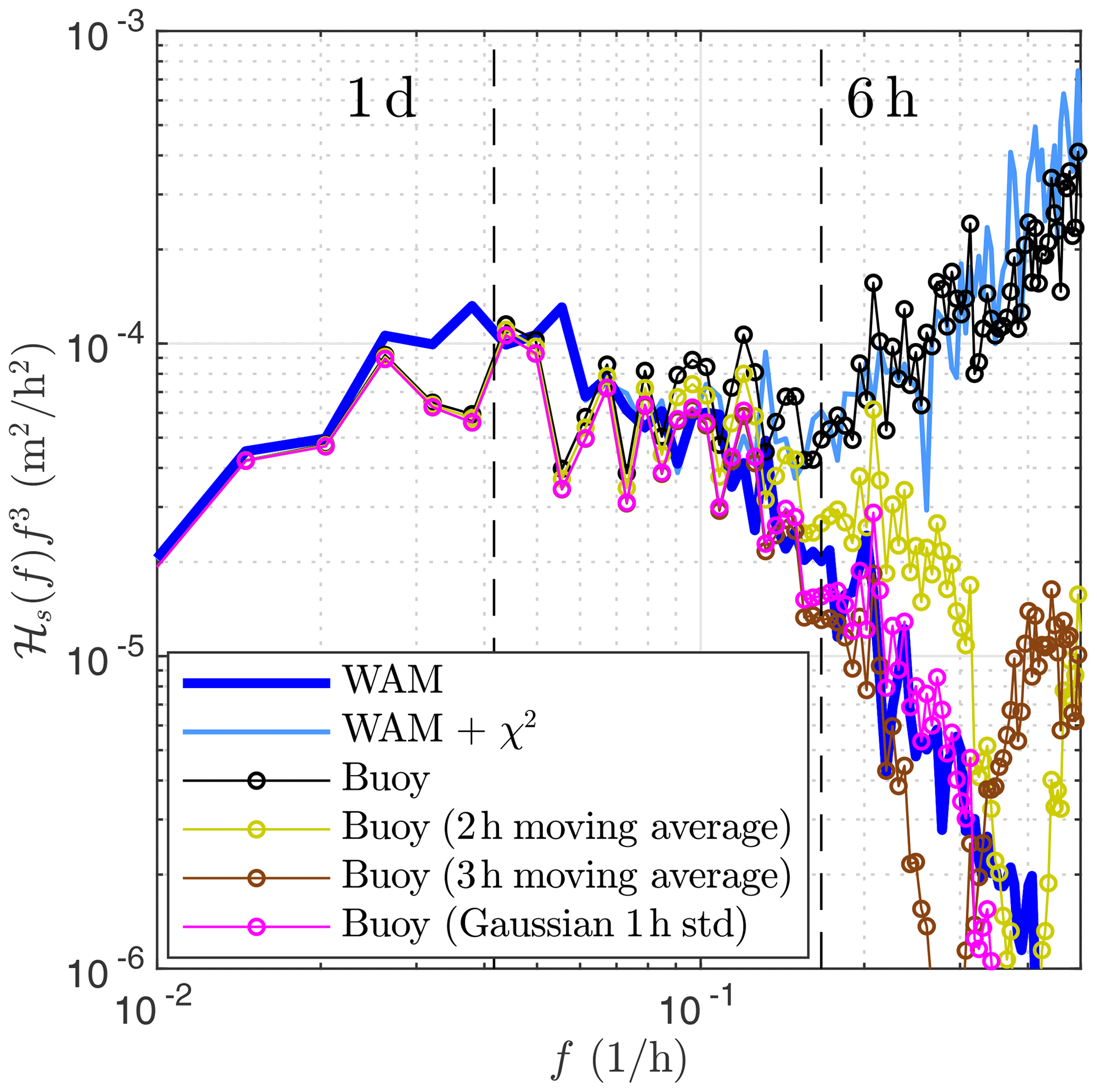
Figure 2A comparison between model data with added sampling variability and observations that have been low-pass filtered by different methods. ℋs(f) is the power spectrum of the significant wave height time series that has been multiplied by f3 to accentuate shorter fluctuations. Data were from a coinciding ice-free period of 28 May 2011–1 February 2012.
3.1.2 Method 2: adding variability to model data
The second approach preserved the original measurements but added random scatter to the model data by assuming that synthetic samples of the wave field variance were χ2-distributed. In other words,
where denotes the sampled variance and dof denotes the degrees of freedom. Following Donelan and Pierson (1983) we used the spectrum to calculate the degrees of freedom for the 8.1 m event (dof =200), which was used throughout. This value was probably too small for low wave conditions but still matched the real scatter of the wave measurements overall (Fig. 2). Also, it was unnecessary to model the scatter of small wave heights precisely, since the distributions were only fitted to the highest values, such as annual maxima.
The artificial samples varied around the deterministic model values, leading to an increase in annual maxima (Fig. 3b–c). Compared to the 7.2 m maximum in the original model data, the highest new maximum in a 100-realisation ensemble was 8.0 m (11 % increase), with the mean of the 100 new maxima being 7.6 m (6 % increase).
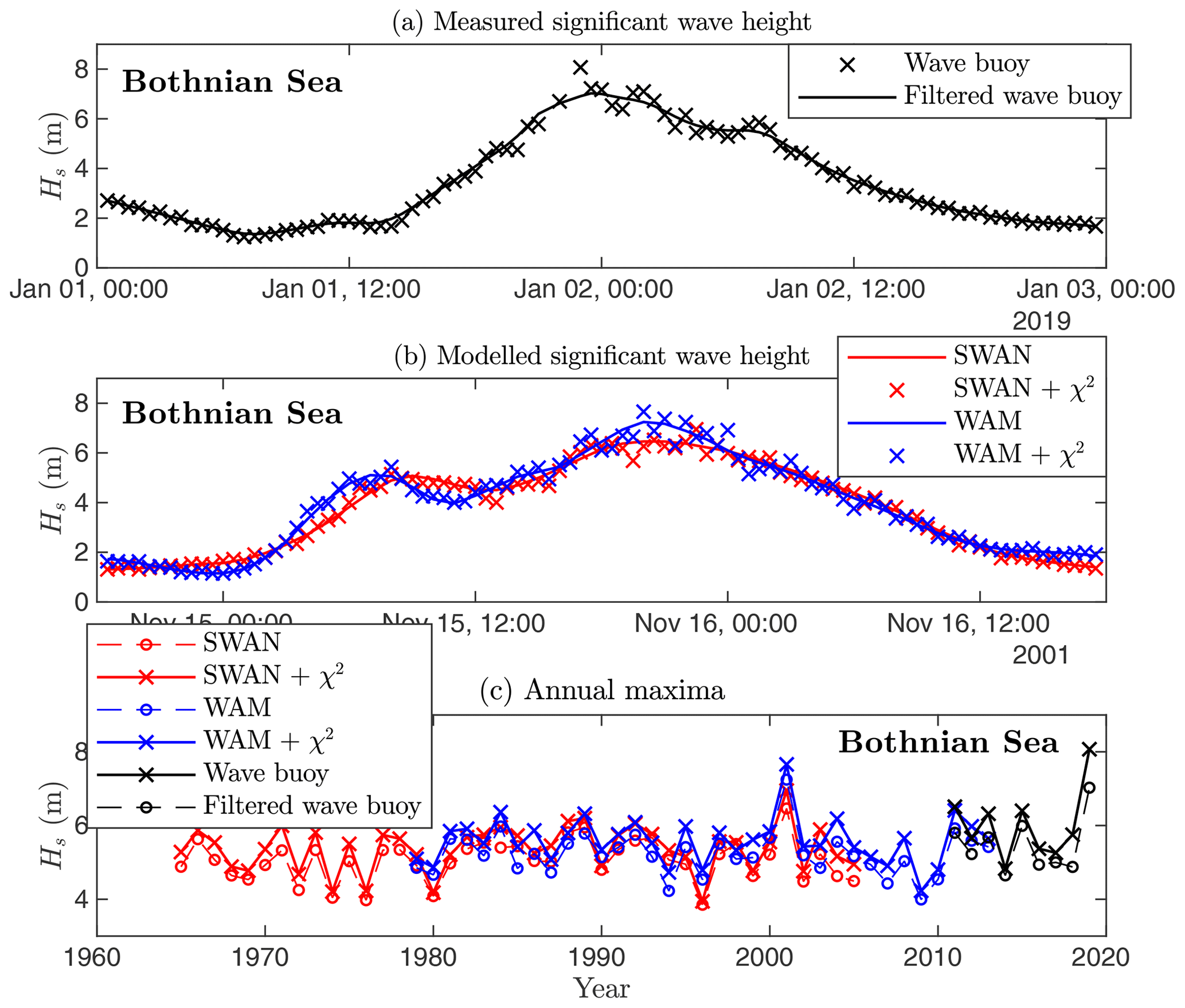
Figure 3Short-term variability removed from observations through low-pass filtering (a). Artificial χ2-distributed samples added to the wave model data from the most severe storm in the hindcasts (b). In both instances annual maxima increase when calculated from data with variability (c).
3.2 Combined measurement–model time series
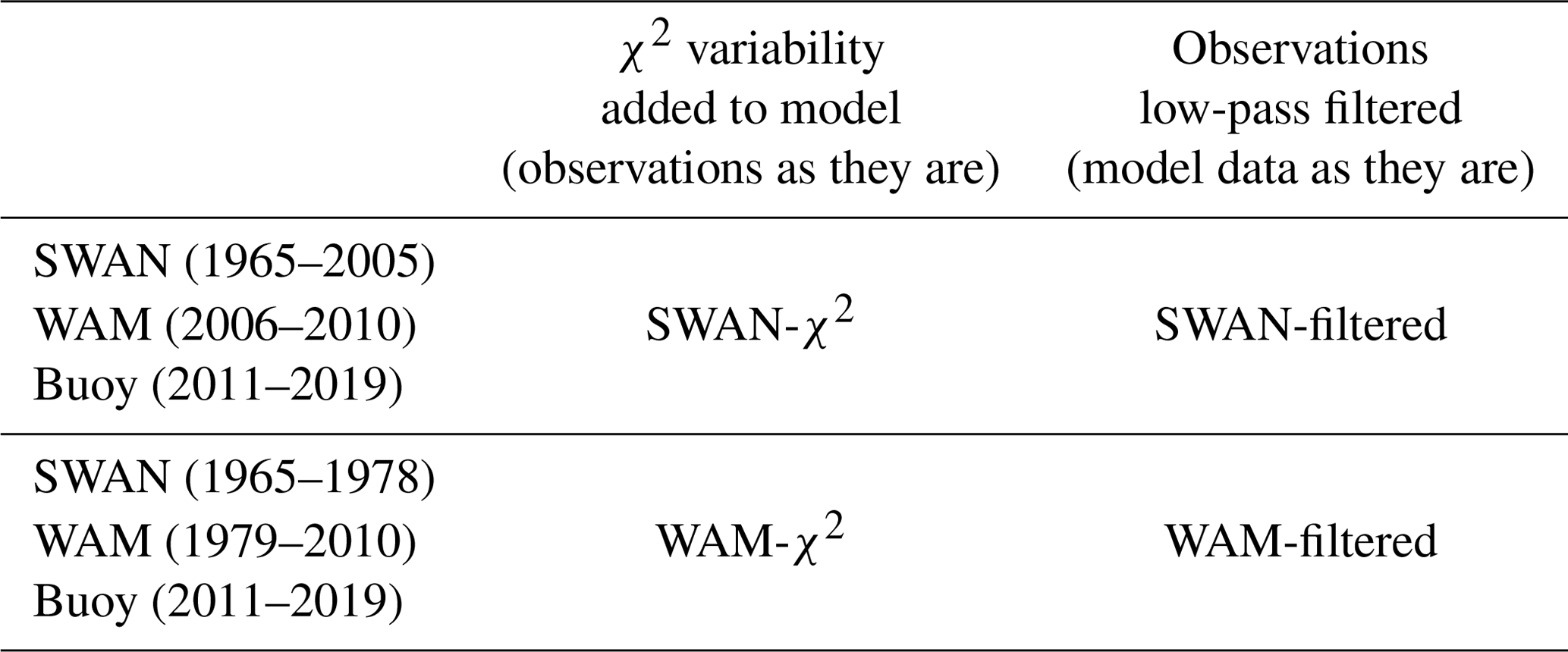
We constructed 55-year time series at the Bothnian Sea wave buoy from the 2011–2019 wave buoy data, the 1965–2005 SWAN hindcast, and the 1979–2013 WAM hindcast. Model data were used for 1965–2010 by choosing one hindcast as the primary source of data and completing the time series using the other one. We then accounted for the difference in sampling variability by either low-pass filtering the measurements (Sect. 3.1.1) or by adding synthetic χ2 sampling variability to the model data (Sect. 3.1.2).
The four resulting time series are denoted SWAN-χ2, SWAN-filtered, WAM-χ2, and WAM-filtered, according to the primary wave hindcast and the method used to account for the sampling variability (Table 1). For the χ2 data sets the results were an average of a 100-realisation ensemble.
Table 1The four different 55-year time series. First, either the SWAN or the WAM hindcast was used as the primary source of model data. Second, two alternative methods to account for the difference in sampling variability between observations and model data were applied (see Sect. 3.1). The data set with the added χ2 variability was a 100-realisation ensemble.
3.3 Fitting distributions and inferring return periods
Block maxima, X, can converge only to a member in the family of generalised extreme value (GEV) distributions (e.g. Coles, 2001), having a cumulative distribution function (CDF) of
where μ is the location parameter, σ is the scale parameter, and ξ is the shape parameter. A negative value of ξ means a thin-tailed distribution, and for ξ=0 Eq. (2) equals the Gumbel distribution.
The second set of distributions were fitted to peak-over-threshold (POT) data, where the original data, x, were converted to values exceeding a fixed threshold, u, i.e. . The maximum values of y were chosen and a minimum distance of 24 h between two values was imposed to insure independence. These data can converge only towards a generalised Pareto distribution (GPD) (e.g. Coles, 2001) with a CDF of
with the meaning of the parameters as for Eq. (2). For ξ=0, H(y) equals the exponential distribution.
We fitted these theoretical distributions to our data using the maximum likelihood method. In the POT method we used the thresholds 4, 4.5, and 5 m, which correspond to percentiles 99.5–99.9 in the combined data sets.
We inferred the return period by evaluating the CDF for the maximum storm wave height and calculating the return period (RP) in years as (e.g. Holthuijsen, 2007)
where T0 is the average time (in years) between two storms.
For the Gumbel and exponential fits the 95 % confidence intervals were determined from the confidence limits of the CDF. For the three-parameter distributions we used the 95 % confidence limits of the shape parameter ξ (Table 2) and the best estimates of the other parameters.
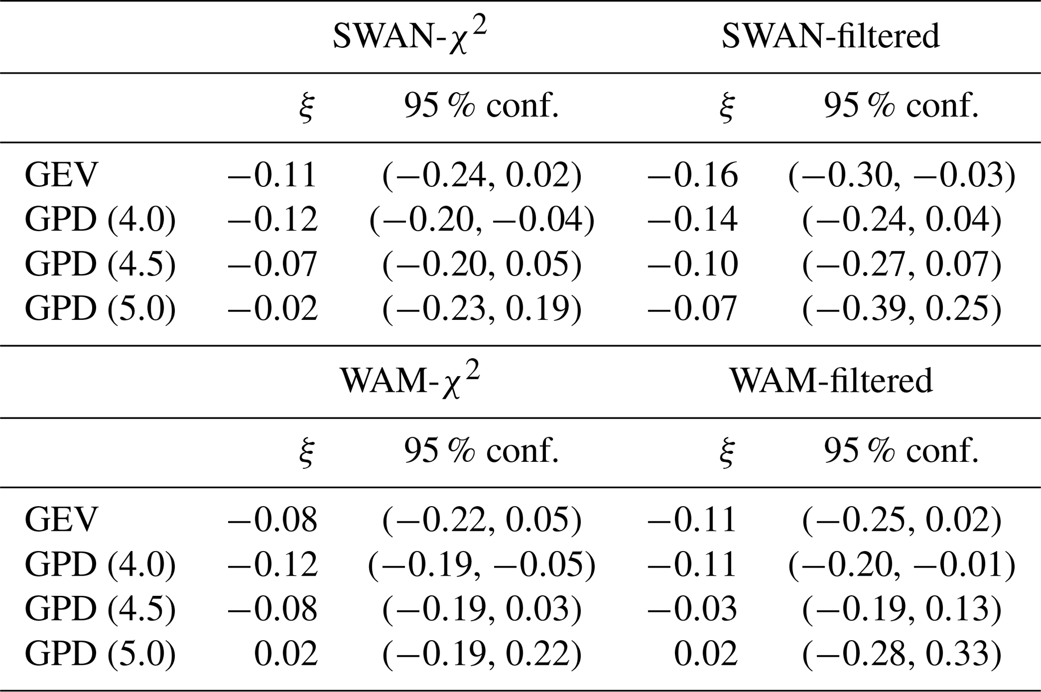
Table 2The shape parameters, ξ, of GEV and GPD fits to annual maxima an POT data, where GPD (4.0) denotes a u=4.0 m threshold for the POT. A negative value of ξ means a thin-tailed distribution. For a description of the data sets (e.g. WAM-χ2), see Table 1.
4.1 Storm track and wind fields
On 28 December 2018 the storm started to develop over the Atlantic ocean close to 40∘ N latitudes (Fig. 1). During the first couple of days the low-pressure system deepened, then weakened, and finally split, with the northern part moving towards Iceland. Near Iceland the cyclone started to deepen again and moved northeast towards northern Scandinavia. After reaching the northern shore of Bay of Bothnia the storm centre dove south and moved over Finland on 1 January 2019. When reaching Estonia the storm had already weakened, eventually filling up after 3 January.
On 1 January 2019, 21:00 UTC the weather station in the northern Bothnian Sea (Valassaaret, Fig. 1) measured a 29.1 m s−1 wind speed from roughly 35∘. Although the prevailing wind direction is south-southwest, the strongest winds are usually from the northeast. The maximum in the entire Baltic Sea was observed 7 h later at Bogskär, where northerly winds reached 32.5 m s−1. Remotely sensed winds were not available from the peak of the storm, but larger parts of the Baltic Sea were covered in the evening before and the morning after the storm (Fig. 4).
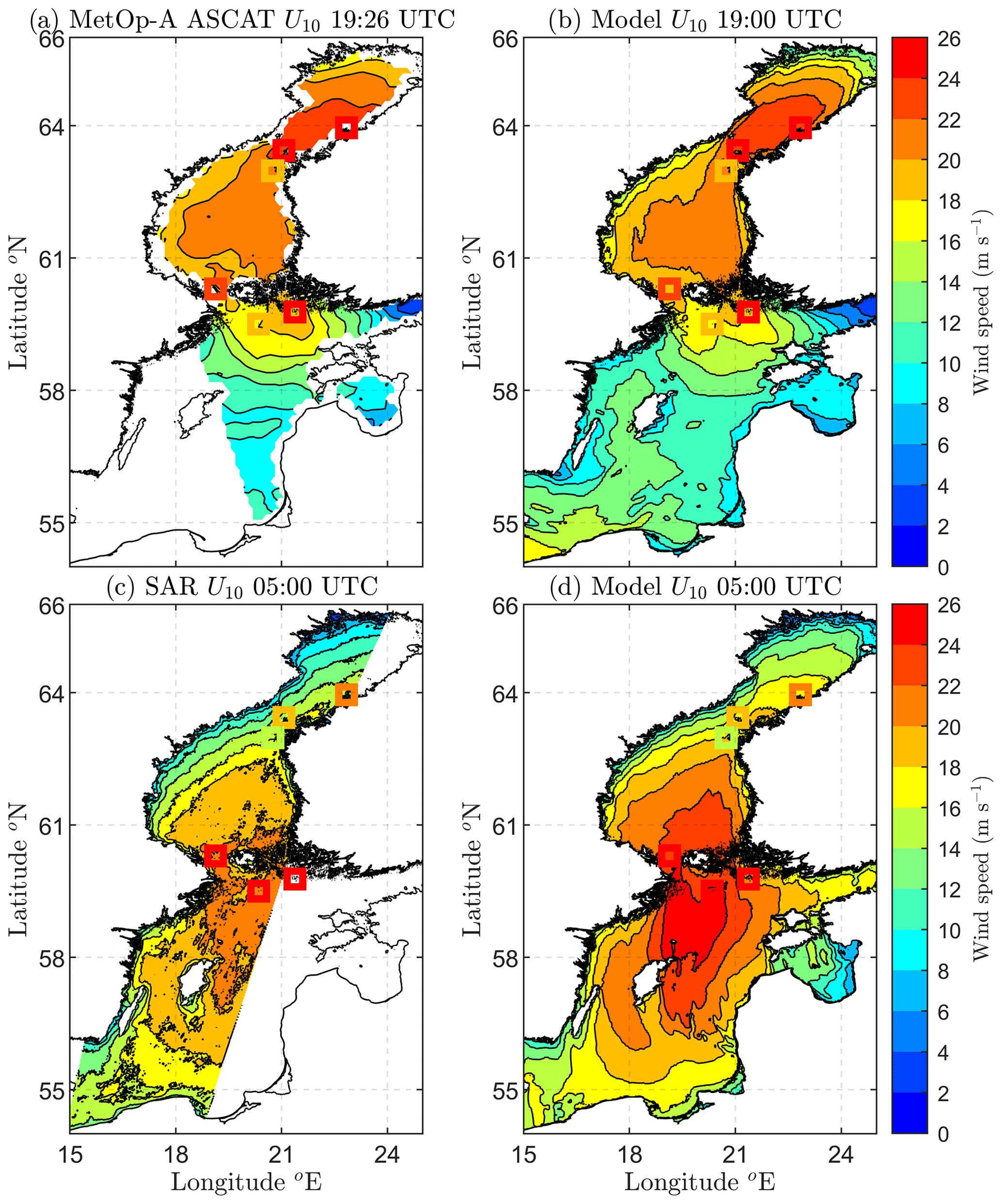
Figure 4Wind speed U10 retrieved from a scatterometer and SAR (a, c) and modelled by HARMONIE (b, d) before and after the storm. The overlaid squares correspond to in situ measurements (from north to south): Tankar, Valassaaret, Strömmingsbäadan, Märket, Utö, and Bogskär.
At 19:00 UTC on 1 January winds north of the Bothnian Sea were blowing 22–24 m s−1 (Fig. 4a–b). The winds of the scatterometer and HARMONIE model products were almost identical, with both also agreeing with the coinciding measurements from the three northernmost weather stations. We surmise that the discrepancy at the Utö station (just south of the Archipelago Sea) was caused by the incomplete treatment of islands in the level-3 processing of the scatterometer product. Nonetheless, this error seems local, as both products match the measured wind speed from Bogskär, located slightly west-southwest of Utö.
At 05:00 UTC the next morning the winds with a maximum intensity of over 24 m s−1 had moved past the Bothnian Sea to the northern Baltic Proper (Fig. 4c–d). Although both SAR and HARMONIE show similar large-scale patterns, the wind speeds from SAR are systematically lower. This is probably indicative of too weak SAR winds, since overall HARMONIE agrees better with the coinciding weather station measurements. SAR's slight underestimation of higher wind speeds in the Baltic Sea is in line with a previous validation by Rikka et al. (2018).
In summary, the modelled HARMONIE winds were in good accordance with both the remote sensing products and weather station data. The comparison also confirmed what was suggested by the in situ measurements, namely that the cyclone generated strong winds along the entire Bothnian Sea when travelling south.
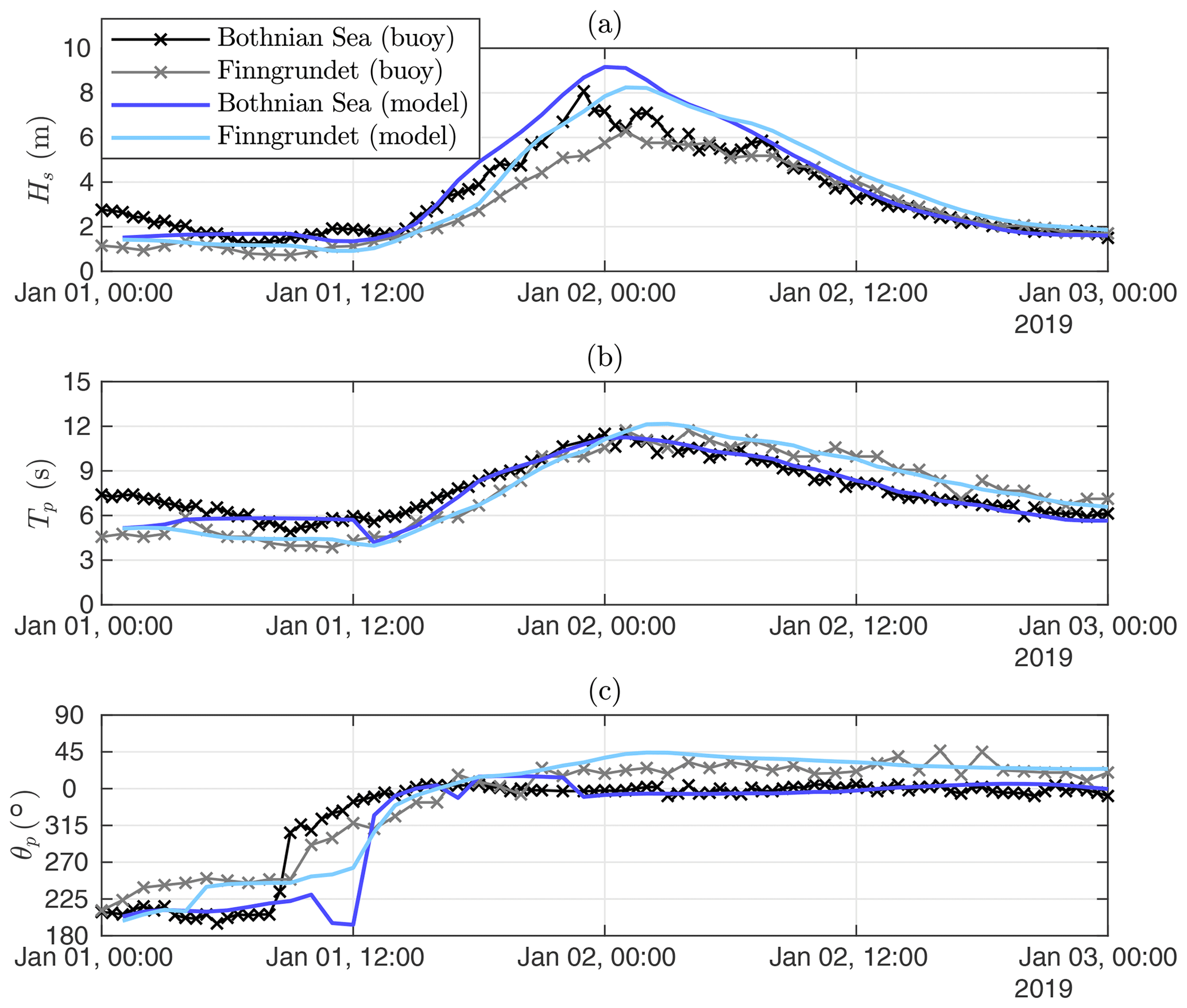
Figure 5The significant wave height (Hs), peak period (Tp), and mean direction at the spectral peak (θp) at the Bothnian Sea and Finngrundet wave buoys. The WAM model hindcast is forced with HARMONIE using a similar set-up as the CMEMS BAL MFC wave forecast. This figure shows the original (non-calibrated) hindcast.
4.2 Waves during the storm
Prior to 2019 the highest significant wave height measured in the Bothnian Sea was 6.5 m (in 26 December 2011). During the storm this value was exceeded for 3.5 h with the significant wave height reaching a maximum of 8.1 m on 1 January 23:00 UTC (Fig. 5, a). This maximum wave height is equal to those measured during storms in the Baltic Proper main basin (Björkqvist et al., 2017). The highest significant wave height at the Finngrundet wave buoy in the southern part of the basin was 6.3 m. The waves in the southern part were lower during the growth phase, but both wave buoys measured similar wave heights during the decay.
The 12 s maximum peak period at Finngrundet equalled that of the Bothnian Sea wave buoy during the height of the storm (Fig. 5b). Nevertheless, during the relaxation of the storm the waves at Finngrundet were up to 2 s longer compared to the Bothnian Sea buoy, which is explained by the difference in fetch. The wave direction at the Bothnian Sea wave buoy was steady from the north, while being from the north-northeast at Finngrundet (Fig. 5c). This 20–30∘ difference was caused by depth-induced wave refraction or the slanting fetch geometry in the basin (Holthuijsen, 1983).
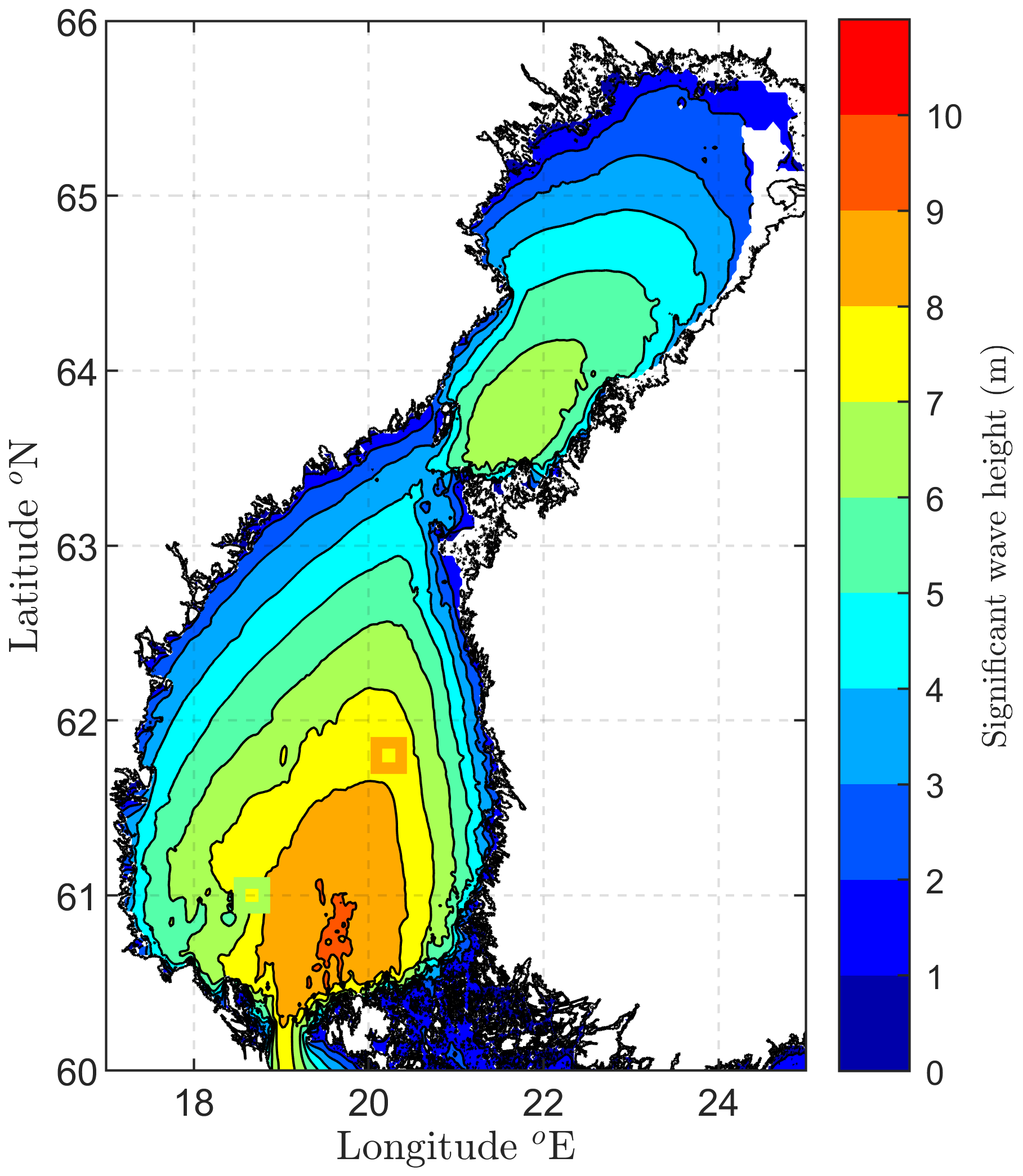
Figure 6The maximum significant wave height for the January 2019 storm from the calibrated wave hindcast. The maximum measured significant wave heights at the Bothnian Sea and Finngrundet wave buoys are shown by overlaid squares.
Basin-wide wave fields from the storm were available from the HARMONIE-forced hindcast, which – while capturing the period and direction accurately – overestimated the significant wave height at both wave buoy locations (Fig. 5). A calibration against Bothnian Sea and Finngrundet buoy observations from 1–3 January determined a 20 % positive model bias in the significant wave height, which was corrected for in the entire Gulf of Bothnia model data. Figure 6 shows that the significant wave height exceeded 8 m in a wide area south of the Bothnian Sea wave buoy, even reaching 9 m in the southernmost part of the basin. We consider these calibrated model results reliable, as they even capture the small-scale features near the Finngrundet buoy accurately. In the Bay of Bothnia (north of the Bothnian Sea, Fig. 1) the significant wave height exceeded 6 m, which is higher than the maximum value of 4.6 m that FMI's wave buoy has measured in the middle part of the basin since 2012. Nevertheless, no wave buoy data were available from the Bay of Bothnia for the storm, and these modelled values are therefore less reliable.
Even though the coast of Bay of Bothnia – including the narrow passage to the Bothnian Sea – typically freezes already in December (SMHI and FIMR, 1982), the sub-basin was almost ice-free on 1 January 2019. We still estimated that the waves propagating from the Bay of Bothnia probably had none to little effect on the sea state at the Bothnian Sea wave buoy (see Appendix A). On the other hand, the coasts of the Bothnian Sea are also frequently frozen in January. If this would have been the case in 2019, the narrower fetch geometry would have lowered the maximum wave height.
We now present results obtained from fitting the theoretical distributions of Sect. 3.3 to the data sets presented in Table 1. On average the GEV and GPD distribution were thin-tailed (ξ<0), with the WAM data sets resulting in slightly higher values for the shape parameter ξ than the SWAN data (Table 2). Nonetheless, the 95 % confidence intervals typically contained ξ=0. The shape parameter of the GPD fit increased with higher thresholds, which indicated that the highest wave heights were better captured by an exponential type distribution (ξ≈0). For the block maxima, the GEV shape parameter typically resembled that of a GPD fit using the lowest threshold u=4.0 m (with the exception of WAM-χ2).
Table 3The estimated return period of the maximum significant wave height at the Bothnian Sea wave buoy during the storm using block maxima and POT data. The notation GPD (4.0) means a u=4.0 m threshold for the POT data. Distributions used for the best estimate and for the return periods in Table 4 are italicised. For a description of the data sets (e.g. WAM-χ2), see Table 1.

Table 3 summarises the return periods estimated from the different distributions and data sets. We make four observations.
-
Fixing ξ=0 vs. GEV and GPD. The negative shape parameters of the general distributions (GEV and GPD) resulted in longer return period estimates compared to the specific distributions (Gumbel and exponential). Increasing the threshold in the POT method resulted in shorter return periods when using the GPD distributions. In contrast, the exponential fits gave longer return periods when the threshold was increased. For the highest threshold, u=5.0 m, the results of the GPDs were close to those of the exponential distributions, which is consistent with ξ being near 0.
-
POT vs. annual maxima. The results from POT data were most consistent with those from annual maxima when using a threshold of 4.5 m (for χ2 data) or 4.0 m (for filtered data). This difference might be explained by the lower values in the filtered data, even though 4.5 m is in the 99.8th percentile for both data sets.
-
Filtered vs. χ2 data. Using filtered data led to consistently shorter estimates for the return period compared to using the χ2 data sets. This was the case for all distributions and both sources of model data (SWAN and WAM). When the specific distributions were fit to filtered data, they gave return periods that were, on average, 64 years (44 %) shorter than for χ2 data. For the general distributions this difference was 309 years (57 %).
-
SWAN vs. WAM hindcast. The general distributions were sensitive to the choice of primary model hindcast: a change from SWAN to WAM reduced the estimates from the GEVs and GPDs by an average of 149 years (40 %). In contrast, the Gumbel and exponential distributions were consistent between the different sources of model data, with a difference of only 6 years (7 %).
The GEV and GPD fits were heavily influenced by significant wave heights below roughly 5 m, thus representing the extremes less accurately than the Gumbel or exponential distributions (Fig. 7). This influence – seen as a downward curvature in the fits of Fig. 7 – was more severe for the GEV compared to the GPD (u=4.5 m). Also, fitting a GPD with a 4.0 m threshold exacerbated the effect (not shown here, but figure available as Supplement; also see Table 3).
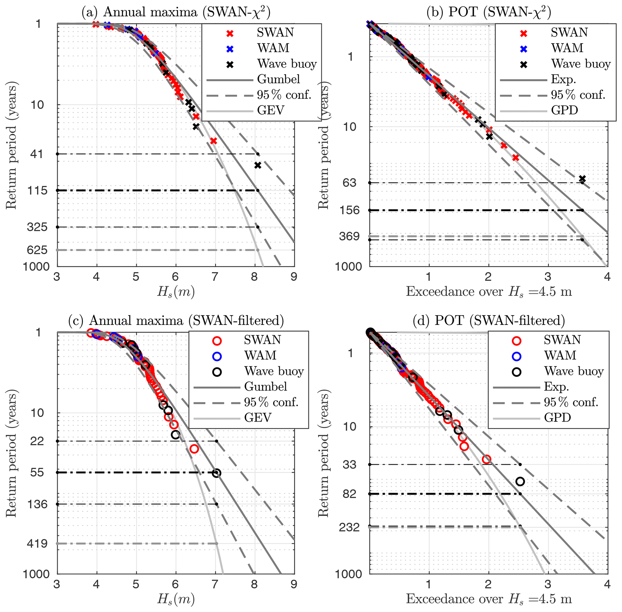
Figure 7Fits to annual maxima and POT values from the Bothnian Sea wave buoy. (a, b) Original observations and model values with an added synthetic χ2 variability. (c, d) Original model data and low-pass-filtered observations. A single realisation of added χ2 variability being close to averages of Table 3 has been chosen. Illustrations of other data combinations and thresholds are available as Supplement.
In summary, the general distributions gave poor fits for the highest values, were sensitive to the choice of model data, and gave up to infinite return periods with the lower-bound ξ values (Table 3). These findings motivated us to discard the GEV and GPD distributions. Fixing ξ=0 was reasonable in the general framework of extreme value theory, since this value was typically included in the confidence intervals of the parameter (Table 2). Restricting ourselves to the Gumbel and exponential distributions, the filtered data gave an average estimated return period of 72 years, with a 95 % confidence of (28, 224), while the respective value using χ2 data was 136 years (50, 423). The grand average using both types of data was 104 years (39, 323) (average of all italicised distributions in Table 3).
Visually, the exponential distributions were good fits for the entire range of significant wave heights when using u= 4.5 m (Fig. 7). The annual maxima showed an “inverse S shape”, which was incompatible with all the theoretical distributions. One reason for the better fit of the exponential distribution compared to the Gumbel distribution was probably the wastefulness of block maxima: there are only 55 annual maxima but 106 POT data points (SWAN-filtered, u= 4.5 m).
All in all, we subjectively deemed the exponential fit with a threshold of u= 4.5 m as the most reliable. Yet, the return period from this distribution – when averaged using all data sets – was 104 years (44, 268), which is practically identical to 104 (39, 323) determined from the larger average (i.e. only fixing ξ= 0 and nothing else). Picking this exact distribution would therefore have been of little consequence.
6.1 Interpreting the results
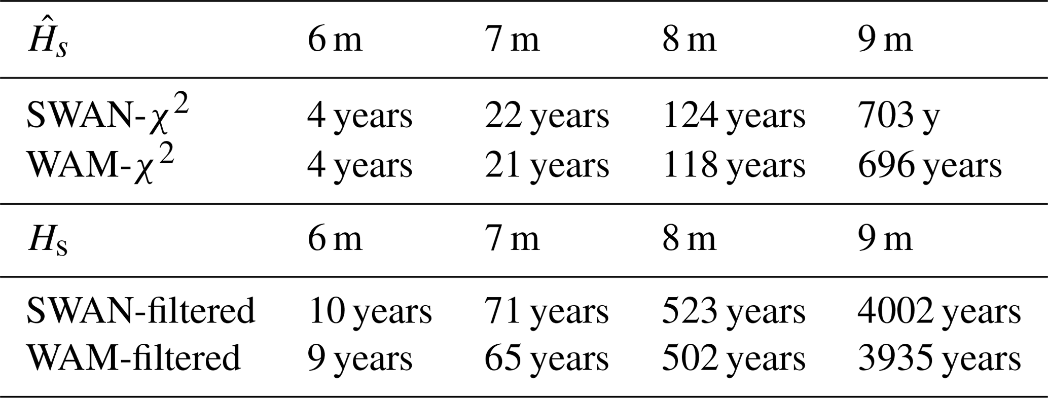
The concept of a return period can be misleading. Correctly interpreted a 100-year return period equals a 1 % annual exceedance probability. Thus, the probability that an event with a 104-year (39, 323) return period actually occurs during the next century is 62 % (27 %, 93 %) – assuming a constant climate. Further, Forristall et al. (1996) and this paper showed that ignoring sampling variability can lead to contradictory results between studies using different types of data. As seen in Table 4, determining return periods of a fixed wave height (instead of return levels for a fixed return period) is especially sensitive to the presence of sampling variability. Specifically, the incidence of a value with sampling variability should not be evaluated against a data set without sampling variability (or vice versa).
Table 4The estimated return period at the Bothnian Sea wave buoy for the significant wave height with sampling variability () and without sampling variability (Hs). Estimates based on averaging distributions with ξ=0 (italicised in Table 3). For a description of the data sets (e.g. WAM-χ2), see Table 1.
Confidence intervals are widely recognised to be an insufficient measure of uncertainty, especially since combining measurements and model data has large possible sources of error. We therefore settled for a simplistic approach for our “best estimate” confidence intervals as an average of the values in the individual distributions. Instead, we focused on other factors and will now discuss our estimates, and the related uncertainties, for the present and future climate.
6.2 Combining the data sets
The ideal low-pass filter does not exist. Therefore, a 3 h smoothing time also removes longer variations from the measurements (Fig. 2), and these variations are most likely physically relevant. It seems like it would be better to preserve the original observations and add χ2 variability to the model data. But if the model data match the (too aggressively) filtered buoy data, it cannot be made fully compatible with the original observations by simply adding random scatter. A gentler filter preserves the properties of the measured wave field better, but at the expense of a more homogeneous measurement–model data set.
By possibly filtering out parts of what made the event unique, the estimated return periods may consequently be biased low. In the WAM-filtered data set the maximum significant wave height was actually 7.2 m, which was modelled by WAM on 15 November 2001 (Fig. 3) – the filtered measured maximum from 2019 was only 7.0 m. On the other hand, the return periods from the χ2 data may be too long; the short-term variations in the model data are inadequate even after the added scatter, thus making all observed events seem rarer than they actually are.
The different time resolution in the wind forcing between the SWAN hindcast (6 h) and the WAM hindcast (1 h) possibly explains some of the differences between their results. The findings of Björkqvist (2020) suggest that a 1 h wind forcing can capture most of the variability in the wave field (aside from random scatter). Nonetheless, Fig. 2 indicates that the WAM hindcast partly suffers from the 3 h temporal resolution of the original ERA-Interim data, even though the wind information was downscaled to a 1 h resolution. Studies using high-temporal-resolution wind products are therefore needed to further study how to optimally combine wave observations and model data.
It is uncertain how much of the discrepancies in the return period estimates are caused by differences between the SWAN and WAM model data sets and how much are caused by possible model biases with respect to the observations. If the latter is more important, then using a single modelled time series might mask uncertainties related to the model performance instead of solving issues related to data inhomogeneity. The matching return periods estimated in Table 4 indicate that possible inhomogeneities between the two model data sets (SWAN vs. WAM) were not a major source of uncertainty if the shape parameter was fixed to ξ=0. Still, as a general recommendation different model data sets should probably be combined only if it is necessary for filling data gaps – as done in this study.
6.3 In the present climate
The cyclone did not follow a typical path that induces southwesterly winds. Instead, it generated strong winds along the longer north–south axis of the Bothnian Sea by approaching the Baltic Sea from the north. While the path is not unique, there are indications that the storm was rare. First, the Bogskär weather station recorded a 32.5 m s−1 10 min average wind speed – the highest value ever measured by FMI in the Baltic Sea. Second, new sea level minima were recorded at all four tide gauges along the Finnish coast of the Bothnian Sea. These stations have been active for almost a century (since 1922, 1925, 1926, and 1933). Therefore, a return period much shorter than our lower-bound estimate of roughly 40 years seems unlikely.
Extreme value theory states that if block maxima converge, then their distribution will be in the GEV family. But yearly blocks are not necessarily long enough for this to happen. Our highest annual maxima were separated from the rest of the data (Fig. 7), possibly because the assumption of drawing from an identical distribution was violated. Then again, the stability of these highest values is infamously poor. Be that as it may, a visual analysis indicates that our extremes were modelled better with the shape parameter fixed to ξ=0 (Gumbel and exponential) than with the general fits (GEV and GPD). We considered the results from the general fits to be unrealistic and back our opinion with a qualitative argument: a half-a-millennium return period is unlikely when the event was observed within 9 years after measurements begun. Also, the 95 % confidence values of the shape parameter, such as 0.24, modelled an infinite return period for a documented event.
Haakenstad et al. (2020) estimated 7–8 m 100-year significant wave heights near the Bothnian Sea wave buoy with a Gumbel distribution (their Fig. 13d), and Aarnes et al. (2012) found similar values using a GEV fit. These studies focused on the northeast Atlantic, thus having a coarse (11 km) model resolution compared to Baltic Sea-specific simulations (e.g. Björkqvist et al., 2018). Their results still agree with our Gumbel distribution's 100-year value (roughly 7.5–8.0 m depending on the data set; Fig. 7a and c).
At first glance our GEV fit (419∕647-year return period for a 7.0∕8.1 m event; Fig. 7a and c) contradicts the 100-year estimate of Aarnes et al. (2012). Still, the 100-year significant wave height estimated from our GEV fit was roughly 6.7–7.5 m – again, depending on the data – thus agreeing reasonably well with both Haakenstad et al. (2020) and Aarnes et al. (2012). Estimates of the return period of a rare event are more sensitive to the distribution tail compared to that of return levels (e.g. 100-year wave heights). On the other hand, this means that a thorough return period analysis of a well-documented event can give valuable information about how plausible different tails of distributions are.
One possible reason for the more erratic nature of the GEV and GPD fits might be issues with data homogeneity; the measured maximum will be a stronger outlier if the model has a negative bias. This especially affects the GEV and GPD distributions, since the shape is mostly determined by the larger number of less extreme values, therefore representing extremes more poorly (Fig. 7). The return period estimates of Table 3 support this interpretation, since the SWAN model had generally lower annual maxima (Fig. 3c). When fixing ξ=0, the results derived from the different model data sets (SWAN vs. WAM) were consistent (Table 4). Thus, we tentatively conclude that distributions with fewer parameters should be preferred if the data are not completely homogeneous.
6.4 In a future climate
No long-term historical trend in Baltic Sea wave heights has been reliably documented. Rather, different studies using disparate data of variable quality have gotten conflicting results (e.g. Broman et al., 2006; Zaitseva-Pärnaste et al., 2009; Räämet et al., 2010). Groll et al. (2017) did project an increase in median significant wave heights – but not extreme values – for 1961–2100. The lack of a trend in annual maxima is consistent with our Bothnian Sea data, but only if observation uncertainty is accounted for properly; ignoring the sampling variability creates a spurious 1.5 cm yr−1 trend – an 80 cm increase over the 55-year time series. This trend vanishes if the data are treated with either method outlined in this paper.
A pseudo-climate study by Mäll et al. (2020) reported an expanding area of extreme waves for past Baltic Sea cyclones under the RCP8.5 emission scenario. While the results were not conclusive, and included no north-to-south cyclones, it is possible that the 2019 storm could respond in a similar way. On a local scale, the strongest (predominantly northeasterly) winds in the northern Bothnian Sea have been projected to shift anti-clockwise (Ruosteenoja et al., 2019). On a broader scale, the shrinking Arctic ice cover (Boé et al., 2009; David et al., 2020) leads to a higher latent heat transport from an open and warmer ocean. Still, we can only speculate how the likelihood or strength of storms resembling that of January 2019 could be affected by meteorological changes.
What is more certain is that the seasonal ice cover of the Baltic Sea is declining (e.g. Vihma and Haapala, 2009). In the present climate the mean annual maximum ice extent covers the entire Bothnian Sea (SMHI and FIMR, 1982; Höglund et al., 2017). The ice-free Bothnian Sea on 1 January 2019 corresponded to average conditions projected under RCP8.5, but a retreat is also projected under the more moderate RCP4.5 scenario (Höglund et al., 2017). A declining ice cover will lead to longer fetches appearing more often. The maximum wave height in January 2019 was adequately modelled using only the wind speed and the Bothnian Sea fetch (Appendix A), and growth curves could therefore be used to quantify the response of the highest waves in the Bothnian Sea to its declining seasonal ice cover.
We investigated methods to combine wave measurements (containing sampling variability) and wave model results (without sampling variability) into a coherent time series. This study was motivated by the need to compensate for insufficient measurement data in order to more reliably estimate the return period of a wave event. The wave event in question caught our interest because it exceeded previously measured and simulated values in the Bothnian Sea sub-basin of the Baltic Sea. During the storm the highest wind speed of 32.5 m s−1 was measured in the Baltic Proper main basin, and the maximum significant wave height of 8.1 m was measured in the Bothnian Sea. Nonetheless, a hindcast specifically calibrated for the storm indicated that the significant wave height reached 9 m in the southern Bothnian Sea (Fig. 6).
To estimate the return period of the event, we covered the time 1965–2019 with 9 years of wave measurements and two long-term wave model hindcasts, and combined them into two types of data:
-
without sampling variability (observations low-pass filtered, model values as they are),
-
with sampling variability (synthetic variability added to model, observations as they are).
The GEV and GPD distributions modelled unrealistically long return periods and were sensitive to the choice of wave hindcast product, possibly because the combined data set was not completely homogeneous. The highest significant wave heights were best captured with a shape parameter close to ξ=0, and we therefore used the Gumbel and exponential distributions to estimate the return period of the storm wave event.
Both methods to account for the difference in sampling variability had their strengths and weaknesses, and it is still uncertain how to best combine modelled and measured wave height data. Averaging the results from both methods, we estimated that the return period was 104 years (95 % conf. 39–323 years). The estimate was 32 years longer (or shorter) if we only used data with (or without) sampling variability.
Although the impact of meteorological changes in the Baltic Sea are uncertain, we surmise that the declining seasonal ice cover will result in wave events of this magnitude becoming more frequent. Additional studies are required to confirm this assertion and to quantify the effect of the retreating seasonal ice.
In conclusion, we found that properly accounting for the lack of sampling variability in model data is crucial if they are used for extreme value analysis in combination with in situ measurements. The different nature of modelled and measured wave data is universal and should, in principle, be taken into account in all studies where they are combined. Nevertheless, the uncertainty of the combination process remains large, further highlighting the value of long, homogeneous, observational time series. Future studies on this topic should use waves that have been modelled using wind data with a high native time resolution, preferably no longer than 1 h.
A1 Hypothetical ice mask in the wave model
We implemented the HARMONIE forced wave model with a hypothetical ice mask covering the entire Bay of Bothnia and compared the results to the original hindcast. The modelled significant wave height and peak period at the Bothnian Sea wave buoy were identical between the two model runs, suggesting that the waves propagating from the Bay of Bothnia to the Bothnian Sea play a negligible part in the Bothnian Sea south of the wave buoy.
A2 Fetch limited wave growth in the Bothnian Sea
The wind speed at a Valassaaret weather station between the Bothnian Sea and the Bay of Bothnia (Fig. 1) during the peak of the storm (U>25 m s−1) was 26.8 m s−1. A wind speed of U=27 m s−1 is compatible with the measured wave spectrum at the height of the storm (Fig. A1) when considering the equilibrium constant and the power-law transition frequency (Phillips, 1958; Kahma, 1981; Kahma and Calkoen, 1992). The directional spreading at the spectral peak was 16∘, and we therefore determined the 194 km northerly fetch as an average over a 30∘ sector.
A 27 m s−1 wind speed would result in a peak period of 11 s (composite data set; Kahma and Calkoen, 1992). This is in reasonable agreement with the measured value of 12 s. Assuming the aforementioned wind speed and fetch, the locally generated significant wave height in the Bothnian Sea would have been 7.4 m. Although this is less than the measured value of 8.1 m, it is a fair match to the low-pass-filtered maximum of 7.0 m.
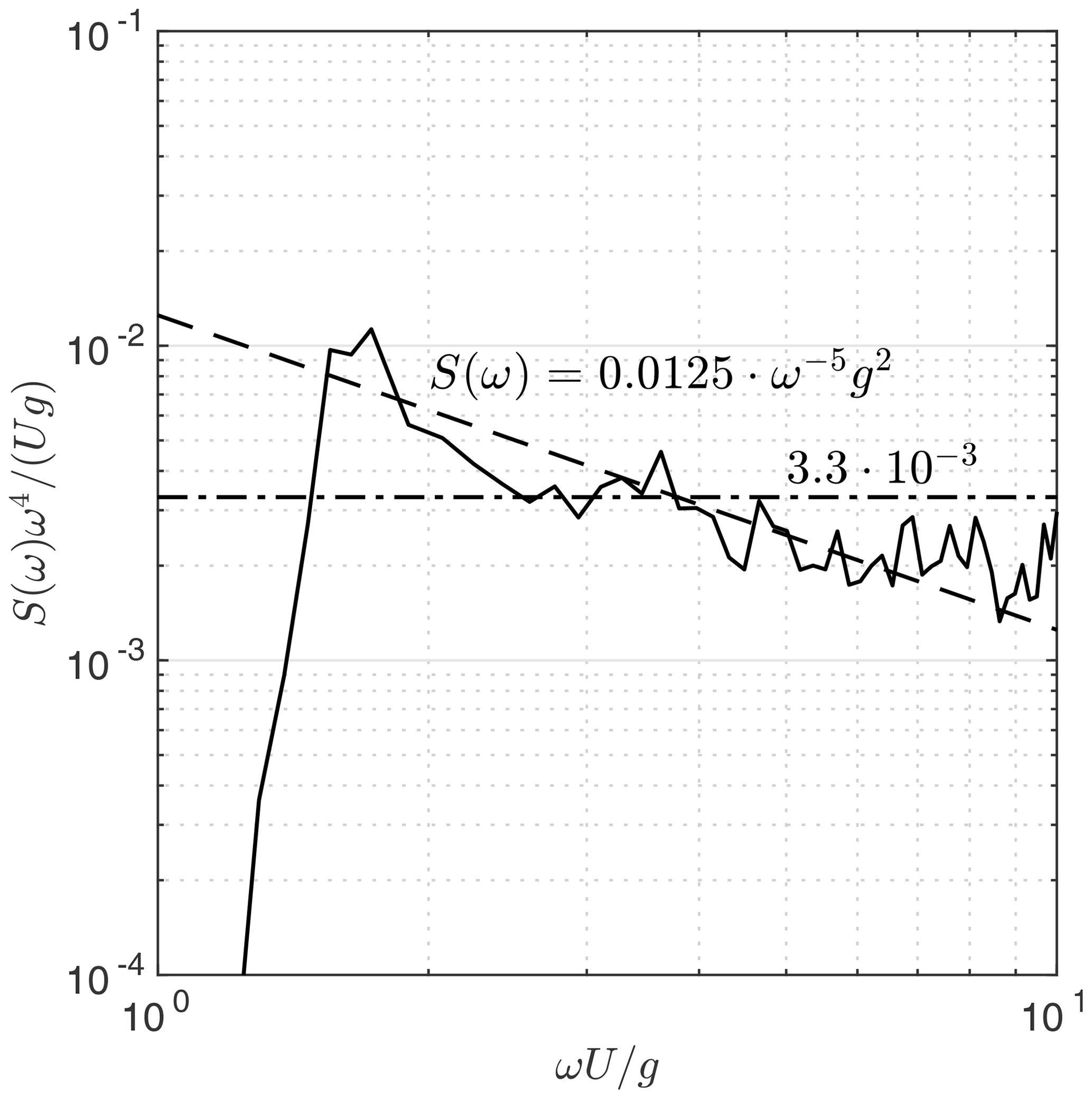
Figure A1The wave spectrum measured with the Bothnian Sea wave buoy at the height of the storm (1 January 2019 23:00 UTC). The spectrum has been scaled assuming a wind speed of U=27 m s−1. The equilibrium level (dashed–dotted) and the saturation level (dashed) are also shown.
The wave time series for the Bothnian Sea wave buoy location are published as an open data set (Björkqvist et al., 2020). The Finngrundet wave measurements are available from the SMHI open data portal (https://opendata-download-ocobs.smhi.se/explore/, SMHI, 2019). The remotely sensed data are available at the Copernicus CMEMS data portal (https://resources.marine.copernicus.eu/?option=com_csw&view=details&product_id=WIND_GLO_WIND_L3_NRT_OBSERVATIONS_012_002, E.U. Copernicus Marine Service Informatio, 2020) and the Copernicus Open Access Hub (https://scihub.copernicus.eu/, Copernicus and ESA, 2020). The distributions were fitted using the Statistics and Machine Learning Toolbox in MATLAB R2018b. The χ2 simulations were performed using the Statistics and Machine Learning Toolbox in MATLAB R2018b. The random number generator was set to “default” to ensure reproducibility.
The supplement related to this article is available online at: https://doi.org/10.5194/nhess-20-3593-2020-supplement.
The paper was initiated by JVB and VA. AM was responsible for the analysis of the meteorological conditions. The in situ wave measurements were analysed by JVB and HP, and remote sensing data were analysed by SR. The additional wave model simulations were performed by LT, and they were reviewed by SR and VA. Statistical analysis was performed by JVB. The manuscript was prepared by JVB, SR, VA, and AM, with contributions from all co-authors.
The authors declare that they have no conflict of interest.
This study has utilised research infrastructure facilities provided by FINMARI (Finnish Marine Research Infrastructure network), E.U. Copernicus Marine Service Information (products BALTICSEA_ANALYSIS_FORECAST_PHY_003_006 & WIND_GLO_WIND_L3_NRT_OBSERVATIONS_012_002), and data provided by the Copernicus Open Access Hub. We acknowledge the effort of Jani Särkkä to post-process and provide the data of the WAM hindcast. Lastly, the authors would like to thank the anonymous reviewers for their comments and suggestions, which helped to further improve the manuscript.
This research has been supported by the Estonian Research Council (grant no. PSG22), the Estonian Ministry of Education and Research (grant no. PUT1378), the Strategic Research Council at the Academy of Finland (grant no. 292 985), and the State Nuclear Waste Management Fund of Finland (VYR) through the Finnish Research Programme on Nuclear Power Plant Safety 2019–2022 (grant no. SAFIR2022).
This paper was edited by Piero Lionello and reviewed by two anonymous referees.
Aarnes, O. J., Breivik, Ø., and Reistad, M.: Wave Extremes in the northeast Atlantic, J. Climate, 25, 1529–1543, https://doi.org/10.1175/JCLI-D-11-00132.1, 2012. a, b, c, d, e
Berg, P., Döscher, R., and Koenigk, T.: Impacts of using spectral nudging on regional climate model RCA4 simulations of the Arctic, Geosci. Model Dev., 6, 849–859, https://doi.org/10.5194/gmd-6-849-2013, 2013. a
Bidlot, J. R., Holmes, D. J., Wittmann, P. A., Lalbeharry, R., and Chen, H. S.:Intercomparison of the performance of operational ocean wave forecasting systems with buoy data, Weather Forecast., 17, 287–310, https://doi.org/10.1175/1520-0434(2002)017<0287:IOTPOO>2.0.CO;2, 2002. a, b
Bitner-Gregersen, E. M. and Magnusson, A. K.: Effect of intrinsic and sampling variability on wave parameters and wave statistics, Ocean Dynam., 64, 1643–1655, https://doi.org/10.1007/s10236-014-0768-8, 2014. a
Björkqvist, J.-V.: Waves in Archipelagos, PhD thesis, FMI Contributions 159, University of Helsinki, Helsinki, Finland, available at: http://hdl.handle.net/10138/308954, last access: 14 December 2020. a
Björkqvist, J.-V., Tuomi, L., Tollman, N., Kangas, A., Pettersson, H., Marjamaa, R., Jokinen, H., and Fortelius, C.: Brief communication: Characteristic properties of extreme wave events observed in the northern Baltic Proper, Baltic Sea, Nat. Hazards Earth Syst. Sci., 17, 1653–1658, https://doi.org/10.5194/nhess-17-1653-2017, 2017. a
Björkqvist, J.-V., Lukas, I., Alari, V., van Vledder, G. Ph., Hulst, S., Pettersson, H., Behrens, A., and Männik, A.: Comparing a 41-year model hindcast with decades of wave measurements from the Baltic Sea, Ocean Eng., 152, 57–71, https://doi.org/10.1016/j.oceaneng.2018.01.048, 2018. a, b, c, d
Björkqvist, J.-V., Alari, V., Tuomi, L., and Pettersson, H.: Measured and modelled significant wave height time series at the Bothnian Sea Wave buoy in the Baltic Sea, Zenodo, https://doi.org/10.5281/zenodo.3878948, 2020. a
Boé, J., Hall, A., and Qu, X.: September sea-ice cover in the Arctic Ocean projected to vanish by 2100, Nat. Geosci., 2, 341–343, https://doi.org/10.1038/ngeo467, 2009. a
Booij, N., Ris, R. C., and Holthuijsen, L. H.: A third-generation wave model for coastal regions: 1. Model description and validation, J. Geophys. Res.-Oceans, 104, 7649–7666, https://doi.org/10.1029/98JC02622, 1999. a
Breivik, Ø., Aarnes, O. J., Bidlot, J. R., Carrasco, A., and Saetra, Ø.: Wave extremes in the northeast Atlantic from ensemble forecasts, J. Climate, 26, 7525–7540, https://doi.org/10.1175/JCLI-D-12-00738.1, 2013. a, b
Broman, B., Hammarklint, T., Rannat, K., Soomere, T., and Valdmann, A.: Trends and extremes of wave fields in the north-eastern part of the Baltic Proper, Oceanologia, 48, 165–184, 2006. a
Caires, S., Swail, V. R., and Wang, X. L.: Projection and analysis of extreme wave climate, J. Climate, 19, 5581–5605, https://doi.org/10.1175/JCLI3918.1, 2006. a
Cavaleri, L.: Wave Modeling—Missing the Peaks, J. Phys. Oceanogr., 39, 2757–2778, https://doi.org/10.1175/2009JPO4067.1, 2009. a
Coles, S.: An Introduction to Statistical Modeling of Extreme Values, Springer, London, https://doi.org/10.1007/978-1-4471-3675-0, 2001. a, b, c
Copernicus and ESA: Copernicus Open Access Hub, https://scihub.copernicus.eu, last access: 11 May 2020. a
David, A., Blockley, E., Bushuk, M., Debernard, J. B., Derepentigny, P., Docquier, D., Fu, N. S., John, C., Jahn, A., Holland, M., Hunke, E., Iovino, D., Khosravi, N., Madec, G., Farrell, S. O., Petty, A., Rana, A., Roach, L., Rosenblum, E., Rousset, C., Semmler, T., Stroeve, J., Tremblay, B., and Toyoda, T.: Arctic Sea Ice in CMIP6, Geophys. Res. Lett., 47, 1–26, https://doi.org/10.1029/2019GL086749, 2020. a
Dee, D. P., Uppala, S. M., Simmons, A. J., Berrisford, P., Poli, P., Kobayashi, S., Andrae, U., Balmaseda, M. A., Balsamo, G., Bauer, P., Bechtold, P., Beljaars, A. C., van de Berg, L., Bidlot, J., Bormann, N., Delsol, C., Dragani, R., Fuentes, M., Geer, A. J., Haimberger, L., Healy, S. B., Hersbach, H., Hólm, E. V., Isaksen, L., Kållberg, P., Köhler, M., Matricardi, M., Mcnally, A. P., Monge-Sanz, B. M., Morcrette, J. J., Park, B. K., Peubey, C., de Rosnay, P., Tavolato, C., Thépaut, J. N., and Vitart, F.: The ERA-Interim reanalysis: Configuration and performance of the data assimilation system, Q. J. Roy. Meteor. Soc., 137, 553–597, https://doi.org/10.1002/qj.828, 2011. a
de Montera, L., Remmers, T., O'Connell, R., and Desmond, C.: Validation of Sentinel-1 offshore winds and average wind power estimation around Ireland, Wind Energ. Sci., 5, 1023–1036, https://doi.org/10.5194/wes-5-1023-2020, 2020. a
Donelan, M. A. and Pierson, W. J.: The Sampling Variability of Estimates of Spectra of Wind-Generated Gravity Waves, J. Geophys. Res., 88, 4381–4392, https://doi.org/10.1029/JC088iC07p04381, 1983. a, b
Driesenaar, T., Bentamy, A., de Kloe, J., Rivas, M. B., and et al., R. G.: Quality Information Document for the Global Ocean Wind Products, Tech. rep., Copernicus Marine Environment Monitoring Service, available at: http://resources.marine.copernicus.eu/documents/QUID/CMEMS-WIND-QUID-012-002-003-005.pdf (last access: 14 December 2020), 2019. a
E.U. Copernicus Marine Service Information: Global Ocean Daily Gridded Sea Surface Winds from Scatterometer, available at: https://resources.marine.copernicus.eu/?option=com_csw&view=details&product_id=WIND_GLO_WIND_L3_NRT_OBSERVATIONS_012_002, last access: 11 May 2020. a
Forristall, G., Heideman, J. C., Leggett, I. M., and Roskam, B.: Effect of Sampling Variability on Hindcast and Measured Wave Heights, J. Waterw. Port C., 5, 216–225, https://doi.org/10.1061/(ASCE)0733-950X(1996)122:5(216), 1996. a, b, c, d
Groll, N., Grabemann, I., Hünicke, B., and Meese, M.: Baltic sea wave conditions under climate change scenarios, Boreal Environ. Res., 22, 1–12, 2017. a, b
Haakenstad, H., Breivik, Ø., Reistad, M., and Aarnes, O. J.: NORA10EI: A revised regional atmosphere-wave hindcast for the North Sea, the Norwegian Sea and the Barents Sea, Int. J. Climatol., 40, 1–27, https://doi.org/10.1002/joc.6458, 2020. a, b, c
Haiden, T., Janousek, M., Bidlot, J. R., Buizza, R., Ferranti, L., Prates, F., and Vitart, F.: Evaluation of ECMWF forecasts, including the 2018 upgrade, Tech. Rep., October 831, ECMWF, 2018. a
Hemer, M. A., Fan, Y., Mori, N., Semedo, A., and Wang, X. L.: Projected changes in wave climate from a multi-model ensemble, Nat. Clim. Change, 3, 471–476, https://doi.org/10.1038/nclimate1791, 2013. a
HIRLAM-B: System Documentation, available at: http://hirlam.org, last access: 14 December 2020. a
Höglund, A., Pemberton, P., Hordoir, R., and Schimanke, S.: Ice conditions for maritime traffic in the Baltic Sea in future climate, Boreal Environ. Res., 22, 245–265, 2017. a, b
Holthuijsen, L.: Observations of the Directional Distribution of Ocean-Wave Energy in Fetch-Limited Conditions, J. Phys. Oceanogr., 13, 191–207, 1983. a
Holthuijsen, L. H.: Waves in Oceanic and Coastal Waters, Cambridge University Press, Cambridge, https://doi.org/10.1017/CBO9780511618536, 2007. a
Kahma, K. K.: A study of the growth of the wave spectrum with fetch, J. Phys. Oceanogr., 11, 1504–1515, 1981. a
Kahma, K. K. and Calkoen, C.: Reconciling discrepancies in the observed growth of wind-generated waves, J. Phys. Oceanogr., 22, 1389–1405, 1992. a, b
Komen, G., Cavaleri, L., Donelan, M., K.Hasselmann, Hasselmaan, S., and Janssen, P.: Dynamics and Modelling of Ocean Waves, Cambridge University Press, Cambridge, 1994. a
Kuik, A. J., van Vledder, G. Ph., Holthuijsen, L. H., and Vledder, G. P. v.: A Method for the Routine Analysis of Pitch-and-Roll Buoy Wave Data, J. Phys. Oceanogr., 18, 1020–1034, https://doi.org/10.1175/1520-0485(1988)018<1020:AMFTRA>2.0.CO;2, 1988. a
Longuet-Higgins, M. S.: On the Statistical Distribution of the Heights of Sea Waves, J. Mar. Res., 11, 245–266, 1952. a
Luhamaa, A., Kimmel, K., Männik, A., and Room, R.: High resolution re-analysis for the Baltic Sea region during 1965-2005 period, Clim. Dynam., 36, 727–738, https://doi.org/10.1007/s00382-010-0842-y, 2011. a
Mäll, M., Nakamura, R., Suursaar, Ü., and Shibayama, T.: Pseudo-climate modelling study on projected changes in extreme extratropical cyclones, storm waves and surges under CMIP5 multi-model ensemble: Baltic Sea perspective, Nat. Hazard., 102, 67–99, https://doi.org/10.1007/s11069-020-03911-2, 2020. a
Méndez, F. J., Menéndez, M., Luceño, A., and Losada, I. J.: Estimation of the long-term variability of extreme significant wave height using a time-dependent Peak Over Threshold (POT) model, J. Geophys. Res.-Oceans, 111, 1–13, https://doi.org/10.1029/2005JC003344, 2006. a
Mouche, A. and Vincent, P.: CLS-DAR-NT-10-167, Tech. rep., Collecte Localisation Satellites (CLS), available at: https://sentinel.esa.int/documents/247904/3861173/Sentinel-1-Ocean-Wind-Fields-OWI-ATBD.pdf (last access: 14 December 2020), 2019. a
Orimolade, A. P., Haver, S., and Gudmestad, O. T.: Estimation of extreme significant wave heights and the associated uncertainties: A case study using NORA10 hindcast data for the Barents Sea, Mar. Struct., 49, 1–17, https://doi.org/10.1016/j.marstruc.2016.05.004, 2016. a
Phillips, O. M.: The equilibrium range in the spectrum of wind-generated waves, J. Fluid Mech., 4, 426–434, https://doi.org/10.1017/S0022112058000550, 1958. a
Räämet, A., Soomere, T., and Zaitseva-Pärnaste, I.: Variations in extreme wave heights and wave directions in the north-eastern Baltic Sea, in: Proceedings of the Estonian Academy of Sciences, Estonian Academy Publishers, Estonia, 2, 182–192, https://doi.org/10.3176/proc.2010.2.18, 2010. a
Rikka, S., Pleskachevsky, A., Jacobsen, S., Alari, V., and Uiboupin, R.: Meteo-Marine Parameters from Sentinel-1 SAR Imagery: Towards Near Real-Time Services for the Baltic Sea, Remote Sens., 10, 757, https://doi.org/10.3390/rs10050757, 2018. a
Ruosteenoja, K., Vihma, T., and Venäläinen, A.: Projected changes in European and North Atlantic seasonal wind climate derived from CMIP5 simulations, J. Climate, 32, 6467–6490, https://doi.org/10.1175/JCLI-D-19-0023.1, 2019. a
Salcedo-Castro, J., da Silva, N. P., de Camargo, R., Marone, E., and Sepúlveda, H. H.: Estimation of extreme wave height return periods from short-term interpolation of multi-mission satellite data: application to the South Atlantic, Ocean Sci., 14, 911–921, https://doi.org/10.5194/os-14-911-2018, 2018. a
SMHI: SMHI Open Data, available at: https://opendata-download-ocobs.smhi.se/explore/, last access: 20 February 2019. a
SMHI and FIMR: Climatological Ice Atlas for the Baltic Sea, Kattegat, Skagerrak and Lake Vänern (1963–1979), Tech. rep., SMHI and FIMR, Norrköping, 1982. a, b
Soomere, T., Behrens, A., Tuomi, L., and Nielsen, J. W.: Wave conditions in the Baltic Proper and in the Gulf of Finland during windstorm Gudrun, Nat. Hazards Earth Syst. Sci., 8, 37–46, https://doi.org/10.5194/nhess-8-37-2008, 2008. a
Stopa, J. E., Ardhuin, F., and Girard-Ardhuin, F.: Wave climate in the Arctic 1992–2014: seasonality and trends, The Cryosphere, 10, 1605–1629, https://doi.org/10.5194/tc-10-1605-2016, 2016. a
Tuomi, L., Vähä-Piikkiö, O., and Alari, V.: CMEMS Baltic Monitoring and Forecasting Centre: High-resolution wave forecast in the seasonally ice-covered Baltic Sea, in: The 8th International EuroGOOS Conference, 3–5 October 2017, Bergen, Norway, 269–274, 2017. a
Tuomi, L., Kanarik, H., Björkqvist, J.-V., Marjamaa, R., Vainio, J., Hordoir, R., Höglund, A., and Kahma, K. K.: Impact of Ice Data Quality and Treatment on Wave Hindcast Statistics in Seasonally Ice-Covered Seas, Front. Earth Sci., 7, 1–16, https://doi.org/10.3389/feart.2019.00166, 2019. a, b, c, d
Vähä-Piikkiö, O., Tuomi, L., and Huess, V.: Quality Information Document for Baltic Sea Wave Analysis and Forecasting Product, Tech. rep., Copernicus Marine Environment Monitoring Service, available at: http://resources.marine.copernicus.eu/documents/QUID/CMEMS-BAL-QUID-003-010.pdf (last access: 14 December 2020), 2019. a
Verhoef, A.: EUMETSAT OSI SAF, Tech. rep., Royal Netherlands Meteorological Institute, available at: http://projects.knmi.nl/scatterometer/publications/pdf/osisaf_ss3_atbd.pdf (last access: 14 December 2020), 2018. a
Verhoef, A. and Stoffelen, A.: EUMETSAT OSI SAF, Tech. rep., Royal Netherlands Meteorological Institute, available at: http://projects.knmi.nl/scatterometer/publications/pdf/ascat_validation.pdf (last access: 14 December 2020), 2018. a
Vihma, T. and Haapala, J.: Geophysics of sea ice in the Baltic Sea: A review, Prog. Oceanogr., 80, 129–148, https://doi.org/10.1016/j.pocean.2009.02.002, 2009. a
Vincent, P., Bourbigot, M., Johnsen, H., and Piantanida, R.: S1-RS-MDA-52-7441, Tech. rep., Collecte Localisation Satellites (CLS), available at: https://sentinel.esa.int/documents/247904/1877131/Sentinel-1-Product-Specification (last access: 14 December 2020), 2020. a
Young, I. R., Zieger, S., and Babanin, A. V.: Global Trends in Wind Speed, Science, 332, 451–455, https://doi.org/10.1126/science.1197219, 2011. a
Zaitseva-Pärnaste, I., Suursaar, Ü., Kullas, T., Lapimaa, S., and Soomere, T.: Seasonal and Long-term Variations of Wave Conditions in the Northern Baltic Sea, J. Costal Res., I, 277–281, 2009. a
- Abstract
- Introduction
- Data
- Methods
- Overview of the storm
- Estimating the return period
- Discussion
- Conclusions
- Appendix A: Role of waves propagating from the Bay of Bothnia
- Code and data availability
- Author contributions
- Competing interests
- Acknowledgements
- Financial support
- Review statement
- References
- Supplement