Deep learning of the aftershock hysteresis effect based on the elastic dislocation theory

This paper selects fault source models of typical earthquakes across the globe and uses a volume extending 100 km horizontally from each mainshock rupture plane and 50 km vertically as the primary area of earthquake influence for calculation and analysis. A deep neural network is constructed to model the relationship between elastic stress tensor components and aftershock state at multiple timescales, and the model is evaluated. Finally, based on the aftershock hysteresis model, the aftershock hysteresis effect of the Wenchuan earthquake in 2008 and Tohoku earthquake in 2011 is analyzed, and the aftershock hysteresis effect at different depths is compared and analyzed. The correlation between the aftershock hysteresis effect and the Omori formula is also discussed and analyzed. The constructed aftershock hysteresis model has a good fit to the data and can predict the aftershock pattern at multiple timescales after a large earthquake. Compared with the traditional aftershock spatial analysis method, the model is more effective and fully considers the distribution of actual faults, instead of treating the earthquake as a point source. The expansion rate of the aftershock pattern is negatively correlated with time, and the aftershock patterns at all timescales are roughly similar and anisotropic.

1 Introduction

After the occurrence of strong earthquakes, there is often a large number of aftershocks, which constitute the aftershock sequence. The aftershocks can lead to new damage to the area affected by the main earthquake. Therefore, it is necessary to study aftershocks and stimulate further discussion. Stein and Lisowski systematically discussed the influence of the static stress of the main earthquake on the spatial distribution of aftershocks (Stein and Lisowski, 1983). A large number of earthquake examples show that the change in Coulomb stress produced by the main earthquake is greater than 0.01 MPa, readily triggering aftershocks (Harris, 1998; Toda, 2003; Ma et al., 2005). In addition to the Coulomb failure stress change method, the deep learning method is a new emerging method that can address some questions of physical mechanism. The prediction of the aftershock sequence based on the stress state of the crustal medium is also problematic and is a focus of source physics (Jordan and Mitchell, 2015; Lecun et al., 2015). The neural network has the characteristics of a black box, which can avoid the complicated physical mechanisms when predicting the aftershock pattern (Bodri, 2001; Moustra et al., 2011). In 2018, DeVries et al. (2018) proposed a deep neural network to study the spatial distribution of aftershocks following the main earthquake. A neural network classifier based on stress variation was designed by the authors to determine the possibility of a spatial distribution of aftershocks (DeVries et al., 2018). This idea combines traditional physical analysis mechanisms with data-driven machine learning mechanisms, which can improve our understanding of the complex physical mechanism of earthquakes. Kong et al. also analyzed its necessity (Kong et al., 2019).

The distribution of aftershocks is not only related to spatial changes but also to temporal changes (Kapetanidis et al., 2015; Papadimitriou et al., 2018), which may be related to the actual properties of the medium, i.e., the viscoelastic medium and the porous two-phase medium are closer to the actual geological medium than the elastic medium. The hysteresis effect of the viscoelastic medium on stress change, the effect of readjustment of pore fluid on stress change and other time-dependent medium properties are equally important to post-earthquake stress change, which is an issue that is receiving increasing attention in post-earthquake effects research. In the study of the propagation of a seismic wave and its focal mechanism, the earth medium is assumed to be a completely elastic body. Prior to the main earthquake, the crustal medium will be continuously deformed due to the long-term and slow action of tectonic stress. In the process of stress accumulation (Kaviris et al., 2017; Kaviris et al., 2018), the strain energy of the crustal medium will be accumulated continuously and be stored in the crust in the form of elastic strain energy. When the stress intensity is greater than the bearing stress intensity of the crust, the crust will lose its stability. Discontinuous crust will produce displacement at the location of its fracture, forming an earthquake. Sometimes fracture surfaces are produced in some locally continuous areas. Simultaneously, the elastic strain energy stored in the earth's crust will be released in this process. After the occurrence of the main earthquake, the source body and its surrounding medium will return to the steady state. However, because the main earthquake causes a sudden change in the stress state of the medium, the accumulated elastic strain energy in the entire stress field cannot be released completely at once, but it will continue to be accumulated in other areas, and it will ultimately be released in the form of an aftershock sequence. Therefore, there is a hysteresis effect between the aftershock and the main earthquake (Gu et al., 1979). Omori and Utsu proposed the time distribution formulas of aftershocks. However, the formulas are based on statistical significance, which cannot reflect the underlying reason for the change in aftershock distribution over time and cannot spatialize the temporal change in aftershocks (Omori, 1894; Utsu, 1961). Many scholars also analyzed the spatiotemporal distribution characteristics of aftershocks by building a model, for example, the ETAS (epidemic-type aftershock sequence) model proposed by Ogata (Ogata, 1988), the Kagan–Jackson model proposed by Kagan and Jackson (1994) and the model improved by Ogata based on ETAS (Ogata, 1998). In 2009, Wong and Schoenberg (2009) proposed a joint distribution model that parameterized the aftershock location based on the distance and relative angle between aftershocks and mainshocks (Wong and Schoenberg, 2009). All the above spatiotemporal models of aftershocks are all based on point source earthquakes, while the actual earthquake sources are faults. So the distribution of the main fault zone should be considered when predicting the aftershock pattern. Some spatial models also ignore the relative angle or distance between the mainshock and aftershocks. These deficiencies are taken into account when building the new prediction model.

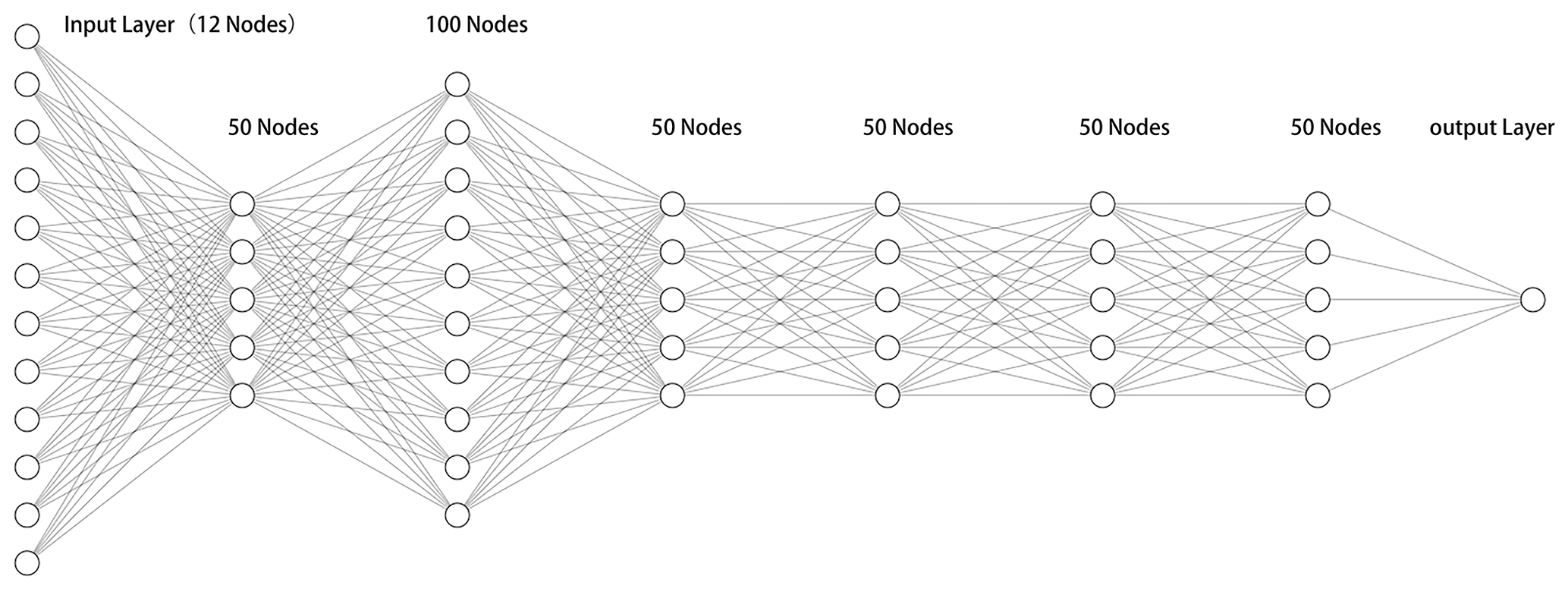
Figure 1 The structure of the DNN (deep neural network). The neural network is composed of an input layer, hidden layers, output layers and the connections between each layer. The function of each hidden layer is to transform the features of the network input.

In this paper, a method based on deep neural networks is proposed to analyze the probability distribution of aftershocks following the main earthquake on multiple timescales, which indirectly reflects the hysteresis effect of aftershocks at different positions under the stress field of the main earthquake. The SRCMOD fault source model database and earthquake events are used as raw data (Mai and Thingbaijam, 2014). First, the analysis area of each main earthquake is gridded, and then the aftershocks of each main earthquake are entered into the grids. The DC3D displacement model is used to calculate the components of stress change tensor for each cell. Based on this grid, the results of the calculation are used as the input to train the neural network, and the aftershock hysteresis model is then obtained. As the application analysis cases for the model, the Wenchuan and the Tohoku earthquakes are not included in the training set or the validation set. Finally, the spatial distribution and expansion characteristics of the aftershock hysteresis model are obtained for both the horizontal and vertical directions. In addition, we focus on two important concepts, namely the “hysteresis effect” and the “aftershock pattern”. The hysteresis effect refers to the change in spatial distribution of aftershocks with the change of timescale. The aftershock pattern refers to the spatial distribution of aftershocks at a certain time.

2 Data and methods

2.1 Data

2.1.1 Raw data

Two types of data are used in this paper, SRCMOD finite fault data and the ISC (International Seismological Centre) earthquake catalogue (Bondár and Storchak, 2011).

The inversion of finite fault source data facilitates a better understanding of the complexity of the earthquake rupture process. Although the spatial resolution of the model is low, it can provide information on deep seismic slip and fault evolution over time. Therefore, the finite fault model is an important means to further study the mechanics and kinematics of the process of earthquake fracture. The online SRCMOD database provides the inversion results for many typical earthquakes from 1906 to present. These results are uploaded by seismologists globally after the main earthquake through inversion. Because the earth's crust is used as an elastic medium in the calculation of coseismic displacement stress, we do not consider the impact of the background of each earthquake. There are 19 finite fault source models used in this analysis: 15 are used as training data, and 4 are used as validation data.

The aftershocks following each main earthquake are obtained from the International Earthquake Center (ISC). More precisely, all aftershock data are from Reviewed ISC Bulletin, which is a subset of the ISC Bulletin that has been manually reviewed by ISC analysts. This includes all events that have been relocated by the ISC. For the mainshock cases in this paper, the aftershocks within 1, 30, 90, 180 and 365 d and within a volume extending 100 km horizontally from each mainshock rupture plane and 50 km vertically are used for analysis of the aftershock sequences.

2.1.2 Data processing

After acquiring the limited fault source data and aftershock sequence data, it is necessary to process them to create the final data for analysis. First, the volume extending 100 km horizontally from each mainshock rupture plane and 50 km vertically is divided into a grid of 5 km³ cubes. Five timescales of aftershock sequence data are then entered into each cube. The aftershock state of a cell with an aftershock is defined as 1, and that of a cell without an aftershock is defined as 0. The final training data have 15 aftershock sequences containing 318 210 subcells, and the validation data have 4 aftershock sequences containing 89 900 subcells.

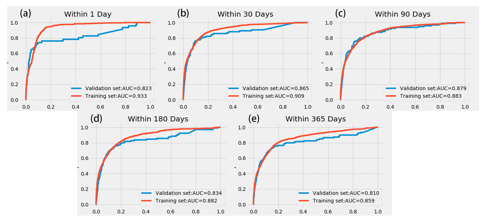
Figure 2 ROC (receiver operating characteristic) curve for multiple timescales. Panels (a) through (e) show the ROC curve of the model within 1, 30, 90, 180 and 365 d, respectively. The horizontal axis represents the FPR (false positive rate), and the vertical axis represents the TPR (true positive rate).

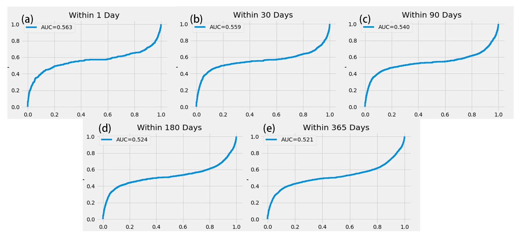
Figure 3 ROC curve of ΔCFS for multiple timescales. Panels (a) through (e) show the ROC curve of the model within 1, 30, 90, 180 and 365 d, respectively. The horizontal axis represents the FPR (false positive rate), and the vertical axis represents the TPR (true positive rate).

2.2 Methods

2.2.1 Okada elastic dislocation theory

The inversion analysis of seismogenic faults after earthquakes is a popular topic in seismology, while in the process of inversion, the application of dislocation theory and models is essential. The dislocation model was first used to analyze fault movement in 1958 (Steketee, 1958). Steketee introduced the dislocation theory into the study of seismic deformation fields and described the relationship between discontinuous displacement on the dislocation plane and the displacement field in an isotropic medium. Okada summarized the existing research in 1985 and proposed a formula for the calculation of displacement in an isotropic, uniform elastic half-space. This formula can be used to calculate the coseismic deformation caused by any fault in the elastic half-space (Okada, 1985, 1992). The Okada dislocation theory systematically summarizes the relationship between point source dislocation and surface deformation caused by rectangular dislocation. The crustal movement is typically slow, and the crustal medium generally shows viscosity and plasticity over a long timescale. At present, the Okada dislocation theory is the most widely used dislocation theory and is often used in combination with InSAR (interferometric synthetic aperture radar) technology. InSAR is used to monitor the surface coseismic deformation field, and the Okada theory is then used to conduct fault slip inversion (Shan et al., 2017; Wang et al., 2018; Cheng et al., 2019; Zhao, 2019).

Therefore, the Okada elastic dislocation theory is used to calculate the coseismic strain stress field of the main earthquake in the paper. The Okada elastic dislocation model, which ignores the influence of stratification in the earth's medium, is widely used in the study of coseismic deformation of the seismic signal source. Okada gives the analytical expression of the partial derivative $\frac{\partial u_i}{\partial x_j}(i,j=\mathrm{1},\mathrm{2},\mathrm{3})$ of the displacement u of the finite fault plane in the elastic half-space (Okada, 1992). This expression is used to obtain the strain tensor ε as

$${\mathit{\epsilon }}_{ij}={\displaystyle \frac{\mathrm{1}}{\mathrm{2}}}\left({\displaystyle \frac{\partial u_i}{\partial x_j}}+{\displaystyle \frac{\partial u_j}{\partial x_i}}\right),$$

and the Lamé constant in the linear solid medium is used to obtain the surrounding stress change tensor σ as

$$\begin{array}{rl}& \mathit{\sigma }=\\ & \left[\begin{array}{lll}\mathit{\lambda }tr\left[\mathit{\epsilon }\right]+\mathrm{2}\mathit{\mu }{\mathit{\epsilon }}_{xx}& \mathrm{2}\mathit{\mu }{\mathit{\epsilon }}_{xy}& \mathrm{2}\mathit{\mu }{\mathit{\epsilon }}_{xz}\\ \mathrm{2}\mathit{\mu }{\mathit{\epsilon }}_{yx}& \mathit{\lambda }tr\left[\mathit{\epsilon }\right]+\mathrm{2}\mathit{\mu }{\mathit{\epsilon }}_{yy}& \mathrm{2}\mathit{\mu }{\mathit{\epsilon }}_{yz}\\ \mathrm{2}\mathit{\mu }{\mathit{\epsilon }}_{zx}& \mathrm{2}\mathit{\mu }{\mathit{\epsilon }}_{zy}& \mathit{\lambda }tr\left[\mathit{\epsilon }\right]+\mathrm{2}\mathit{\mu }{\mathit{\epsilon }}_{zz}\end{array}\right]\end{array},$$

where λ and μ are Lamé constants. In this paper, the crustal medium is regarded as a Poisson body, and the two Lamé coefficients are both 3.0×10¹⁰ Pa. The parameter tr[ε] is the trace of strain tensor ε.

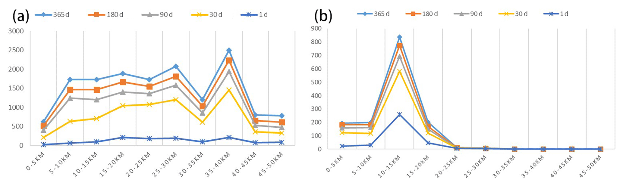
Figure 4 Multi-timescale aftershock depth distribution curves of (a) the Tohoku earthquake and (b) the Wenchuan earthquake.

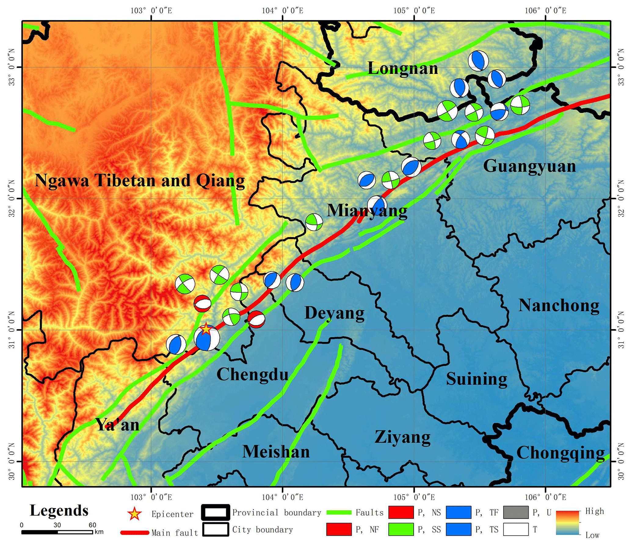
Figure 5 Structural background map of the Wenchuan earthquake. The red and green lines represent the fault structures in this area. The red line is the main fault zone of the Wenchuan earthquake, and the green lines represent other fault zones. The focal mechanism of the main aftershocks are also shown. Ngawa Tibetan and Qiang: Ngawa Tibetan and Qiang Autonomous Prefecture. P, T, NF, NS, SS, TF, TS and U represent tension axis, pressure axis, normal fault, strike-slip normal fault, strike-slip fault, reverse fault, strike-slip reverse fault and unknown type fault, respectively.

2.2.2 DNN

To analyze the hysteresis effect of aftershocks, it is necessary to establish a model that can predict the damage modes of aftershocks at multiple timescales. We constructed a fully connected deep neural network (DNN) to simulate the relationship between the change value of the elastic stress tensor and aftershock and to explain the hysteresis effect of aftershocks. The neural network is based on the extension of the perceptron, and DNN can be understood as a neural network with many hidden layers. A multilayer neural network and deep neural network actually refer to one thing. DNN is sometimes called multilayer perceptron (MLP). The network established here is a network with six hidden layers. Except for the second hidden layer, which has 100 neurons, the other five hidden layers have 50 neurons. The input layer dimension of the entire network is 12. Its input eigenvalue is the combination of the absolute value of six independent components of the elastic stress at the center of each subunit and the negative number of the absolute value, for a total of 12 inputs.

Then we analyze the correlation between aftershocks and stress change, which is closely related to the inputs of DNN. At present, the research on aftershocks is primarily based on statistical methods, and the research content primarily focuses on the distribution of aftershock strength and time attenuation. The intensity distribution of aftershocks follows the G–R (Gutenberg–Richter) relationship $\log N=a-bM$, where M is the magnitude, N is the number of aftershocks with magnitude greater than or equal to M, and a and b are the scale coefficients (Gutenberg and Richter, 1944). The value of b generally varies from 0.6 to 1.1 (Utsu, 2002), and its value is related to the regional stress state (Mogi, 1962; Scholz, 1968).

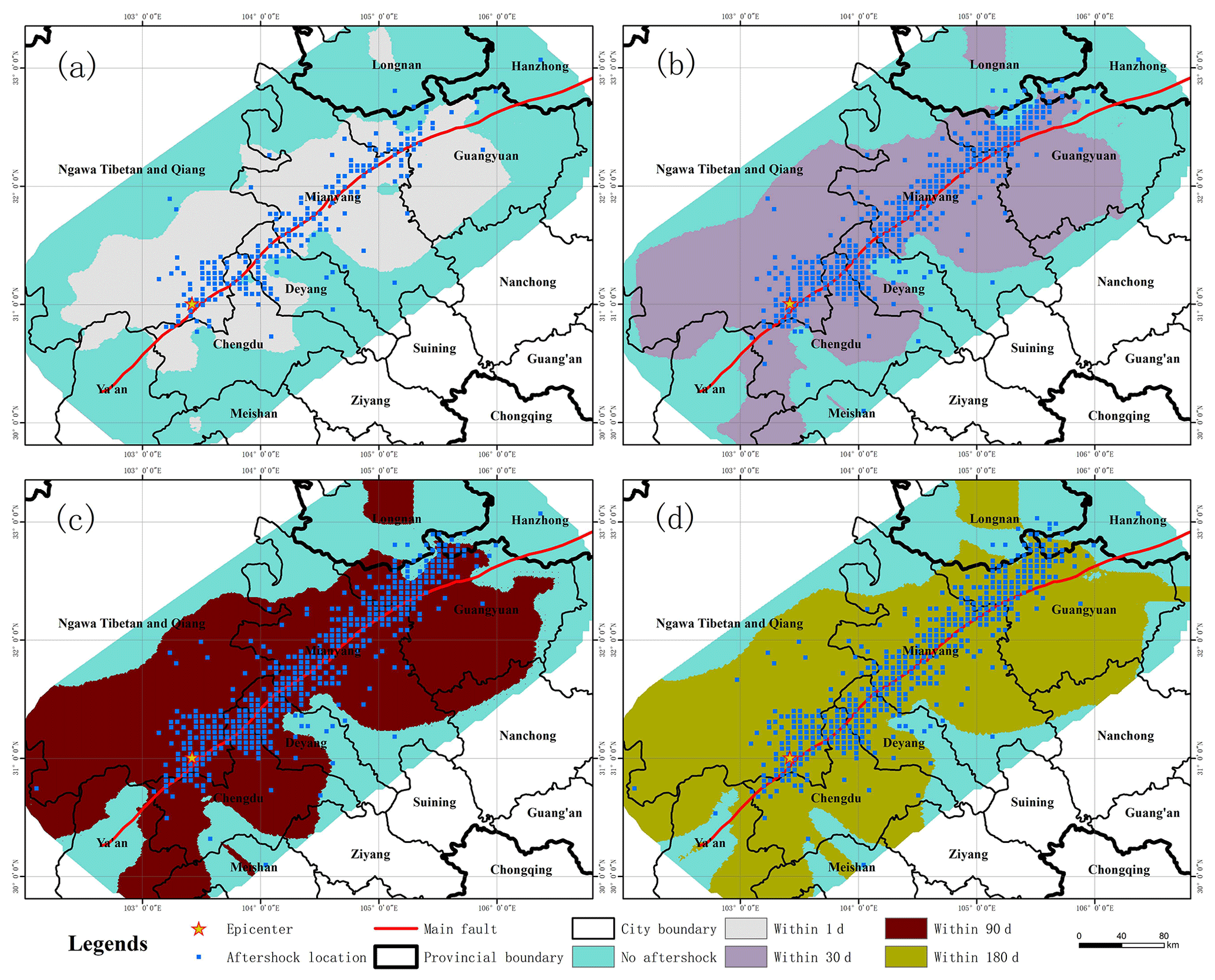
Figure 6 Aftershock damage patterns of the Wenchuan earthquake at multiple timescales. Panels (a) through (d) show the aftershock damage pattern within 1, 30, 90 and 180 d, respectively. The blue dots indicate the actual location of aftershocks at the corresponding timescale.

The study of time attenuation of aftershocks begins with the statistical description of frequency attenuation characteristics of the aftershock sequence using the Omori formula (Omori, 1894). In 1961, Utsu (1961) proposed that the frequency attenuation rate of the actual aftershock sequence is faster than that calculated by the Omori formula (Utsu, 1961) and proposed the modified Omori formula $n\left(t\right)=K(t+c{)}^{-p}$, where n(t) is the aftershock frequency per unit time, c is a constant and p is the attenuation coefficient of the aftershock sequence. For a large number of aftershock sequences, the modified Omori formula accurately describes the time attenuation of aftershocks. In the modified Omori formula, the c value is related to the incomplete recording time after the main earthquake (Kagan and Heidi, 2005), which can provide a physical explanation for the aftershock attenuation after the main earthquake (Lindman et al., 2005). This value is also related to the rupture mode of the main earthquake (Narteau et al., 2009); i.e., the aftershock attenuation is affected by the stress state and related to the stress change.

The stress change caused by the main earthquake can be calculated by the Coulomb fracture stress change, which is also the most widely used analytical method at present. The change in Coulomb stress produced by the main earthquake will trigger the stress of the following aftershocks (Harris, 1998). Some seismologists believe that if the change in Coulomb fracture stress is positive around the main earthquake, it will promote fault movement and trigger aftershocks; if the change in Coulomb fracture stress is negative, it will inhibit fault movement, and the probability of triggering an aftershock is reduced (Lin, 2004; Harris, 1998; Han, 2003). According to the research of DeVries et al., the Coulomb fracture stress change is an inadequate explanation for aftershocks, and the relationship between the positive and negative values of stress change and the triggering of aftershocks requires further exploration. DeVries et al. modeled the relationship between stress change and aftershock triggering by training a neural network (DeVries et al., 2018). The variation in Coulomb fracture stress depends on the geometric properties and coseismic dislocations of the source fault (King et al., 1994; Zhu and Wen, 2009). Therefore, the change value of the stress tensor, which is closely related to the dislocation of the same earthquake, can be used as the aftershock variable to build the model.

In addition, Meade et al. tested many stress-related indicators in 2017 to explain the influence of the coseismic stress field of the main earthquake on the location of aftershocks. Their results show that the sum of the absolute values of the six independent components of the stress tensor, the von Mises yield criterion and the maximum shear stress produce the best interpretation. These variables can be obtained by the combination of the absolute values of the six independent components of the stress tensor and the negative values of the absolute values. Therefore, these variables are also used as the network input (Meade et al., 2017; Mignan and Broccardo, 2019). The input components are expressed as |σ_xx|, |σ_xy|,  |σ_xz|,  |σ_yy|,  |σ_yz|,  |σ_zz|, −|σ_xx|, −|σ_xy|, −|σ_xz|, −|σ_yy|, −|σ_yz| and −|σ_zz|. The dimension of the network output layer is 1, and the output value is the relative probability of aftershocks in each cell, which is between 0 and 1. The dropout layer is also set after each hidden layer. The dropout layer is set to alleviate the occurrence of overfitting in the model training process, which can have a regularization effect. In addition, the activation function of each hidden layer in the network is a ReLU (rectified linear activation) function, and the optimizer is Adadelta. The activation function of the output layer is a sigmoid function, which maps variables between 0 and 1 (Fig. 1). Five scales are analyzed in this paper. Five neural networks are constructed to train five submodels. Each submodel is independent from the others and does not affect the others.

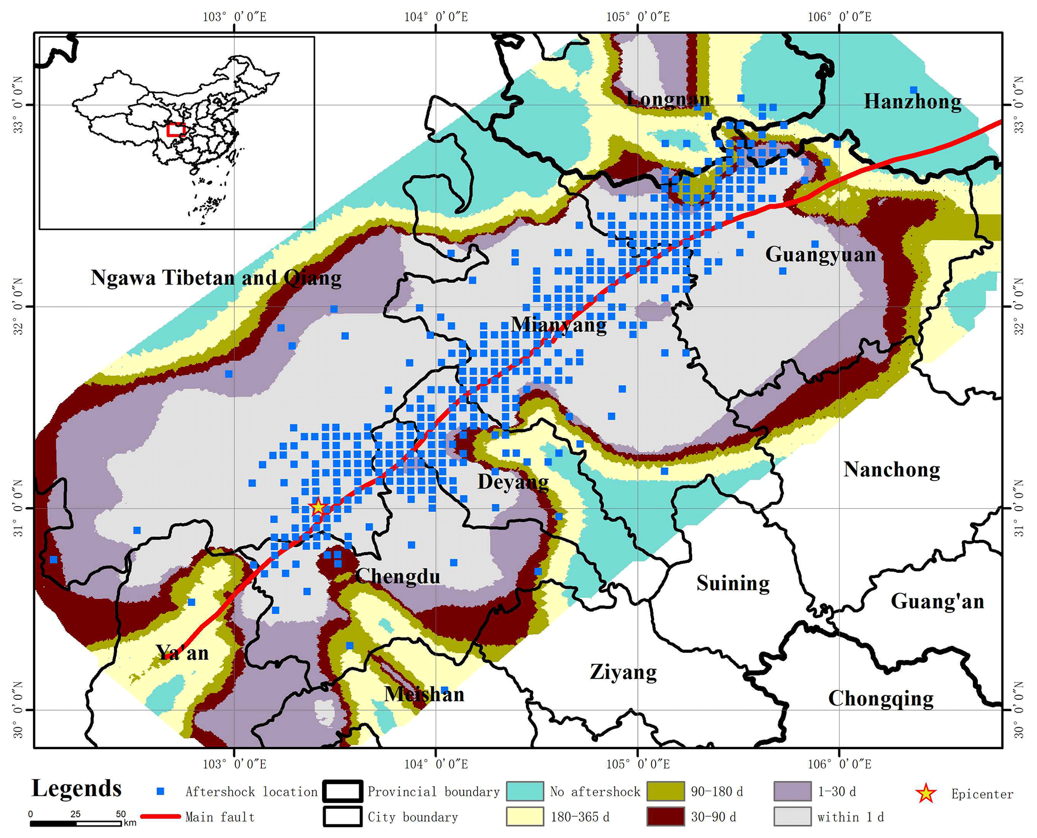
Figure 7 Aftershock hysteresis effect of the Wenchuan earthquake. The aftershock hysteresis effect can be observed by combining the aftershock patterns of the Wenchuan earthquake at different timescales. The blue dots indicate the locations of the actual aftershocks over 1 year.

2.2.3 Model evaluation metric

The ROC (receiver operating characteristic) curve and the AUC (area under curve) are used to evaluate the model. The ROC considers the results obtained under a variety of different criteria. In this article, the ROC curve can reflect the prediction results of the model under multiple thresholds. The AUC is defined as the area enclosed by the coordinate axis under the ROC curve, and the value of the area cannot be greater than 1. Because the ROC curve is generally located above the straight line y=x, the AUC value range is between 0.5 and 1. Based on the AUC value, we can interpret the accuracy of the classifier. When AUC = 1, the classifier is essentially a perfect classifier, whereas when AUC = 0.5, the classifier is making a random assessment, and the obtained model is nonsensical. For the training samples in this paper, there is a class imbalance between positive and negative samples. A characteristic of the ROC curve is that when the distribution of positive and negative samples in the test set changes, the ROC curve can remain unchanged. The closer the ROC curve is to the y axis and y = 1, i.e., the higher the AUC value of the classifier, the greater the classification accuracy is. Generally, when the AUC is less than 0.6, the accuracy of the classifier is poor; when the AUC is less than 0.75, the accuracy of the classifier is moderate; and when the AUC is greater than 0.75, the accuracy of the classifier is good. The output of the model in this paper is a probability value between 0 and 1. When the ROC curve is used to evaluate the model, it is conducted at five timescales, and the model under each timescale is evaluated as a two-classification problem.

Figure 8 Aftershock hysteresis effect of the Wenchuan earthquake in different depths. Panels (a) through (i) show the aftershock hysteresis effect of the Wenchuan earthquake for depth sections of 2.5, 7.5, 12.5, 17.5, 22.5, 27.5, 32.5, 37.5 and 42.5 km, respectively.

3 Results

3.1 Evaluation of the aftershock hysteresis model

The aftershock hysteresis model under multiple timescales is obtained by using the neural network to train the constructed training dataset. In this paper, five submodels are trained, and the final hysteresis model is composed of five submodels. The prediction result given by the model is the approximate range of aftershocks, that is, the position of 5 km³ subcells where aftershocks may occur. Each cell will have a relative probability of aftershocks, which is between 0 and 1. Since this probability value is less than 1 and greater than 0, it does not necessarily mean that aftershocks will occur or that aftershocks will definitely not occur. The output value of the neural network in each cell is binarized with a threshold value of 0.5. A cell with a predicted value greater than 0.5 is assigned as 1, and a cell with a predicted value less than 0.5 is assigned as 0. At locations close to the mainshock, the probability value predicted by the model is more likely to be greater than the threshold 0.5 set in the article.

In this paper, the evaluation-method-based ROC curve is used, and all possible thresholds are taken into account to evaluate the model and physical model in the text. According to the ROC curves of the two methods, the effect of the hysteresis model in the article may be poor under some thresholds, but its AUC value is much greater than that of the physical model. Based on the trained aftershock hysteresis model, the aftershock patterns are predicted for the Wenchuan earthquake at multiple timescales, and the ROC curves are obtained for the different timescales. The AUC values of the five timescales are all above 0.8, in both the training and validation sets, and some are close to 0.9. The AUC values of the training set are all higher than those of the validation set for the different timescales. The neural network designed by DeVries et al. (2018) is used for aftershock prediction. The AUC value of the training model on the validation set is 0.849 (Fig. 2). In this paper, the AUC value of each submodel on the validation set is similar to the research results of DeVries et al. (2018). Therefore, the model achieves good prediction results at different timescales.

For comparison, we forecast the aftershock location based on the static Coulomb failure stress change. Considering the influence of shear stress, normal stress and friction coefficient on the active fault plane, Coulomb failure stress change (ΔCFS) can be expressed as

$$\mathrm{\Delta }\mathrm{CFS}=\mathrm{\Delta }\mathit{\tau }+\mathit{\mu }\mathrm{\Delta }\mathit{\sigma },$$

where μ is the apparent friction coefficient, Δσ is the normal stress on the fault plane and Δτ is the shear stress in the direction of fault slip. Based on previous studies, the friction coefficient in this paper is 0.4 (King et al., 1994; Wan et al., 2004). Numerous studies have shown that aftershocks will occur when ΔCFS is greater than +0.01 MPa. In order to compare and analyze the output of DNN, we need to transform the ΔCFS to 0–1. Similar to the last layer of DNN, the variation function adopts a variant of the sigmoid function as follows:

$$\mathrm{\Delta }\mathrm{CFS}{}^{\prime }={\displaystyle \frac{\mathrm{1}}{(\mathrm{1}+e^{-\mathrm{10}(\mathrm{\Delta }\mathrm{CFS}-\mathrm{0.01})})}},$$

where ΔCFS^′ represents the Coulomb failure stress change after sigmoid transformation. We know that the traditional sigmoid function is similar to the jump function. In the analysis process of this paper, 0.01 MPa is the threshold value to determine whether aftershocks are generated, so the parameter 0.01 in the formula is the translation coefficient; that is, the traditional sigmoid function shifts 0.01 MPa to the right. Parameter 10 is the zoom coefficient, which compresses the sigmoid function horizontally to make its shape approach the jump function as much as possible. When ΔCFS is greater than 0.01 MPa, ΔCFS^′ approaches 1 as much as possible, and when ΔCFS is less than 0.01 MPa, ΔCFS^′ approaches 0 as much as possible. Then we evaluated the results and calculated the AUC value on each timescale by the ROC curve. Compared with the results of the previous model, the AUC results obtained by the method based on static Coulomb failure stress change are generally poor, which are no more than 0.6 (Fig. 3).

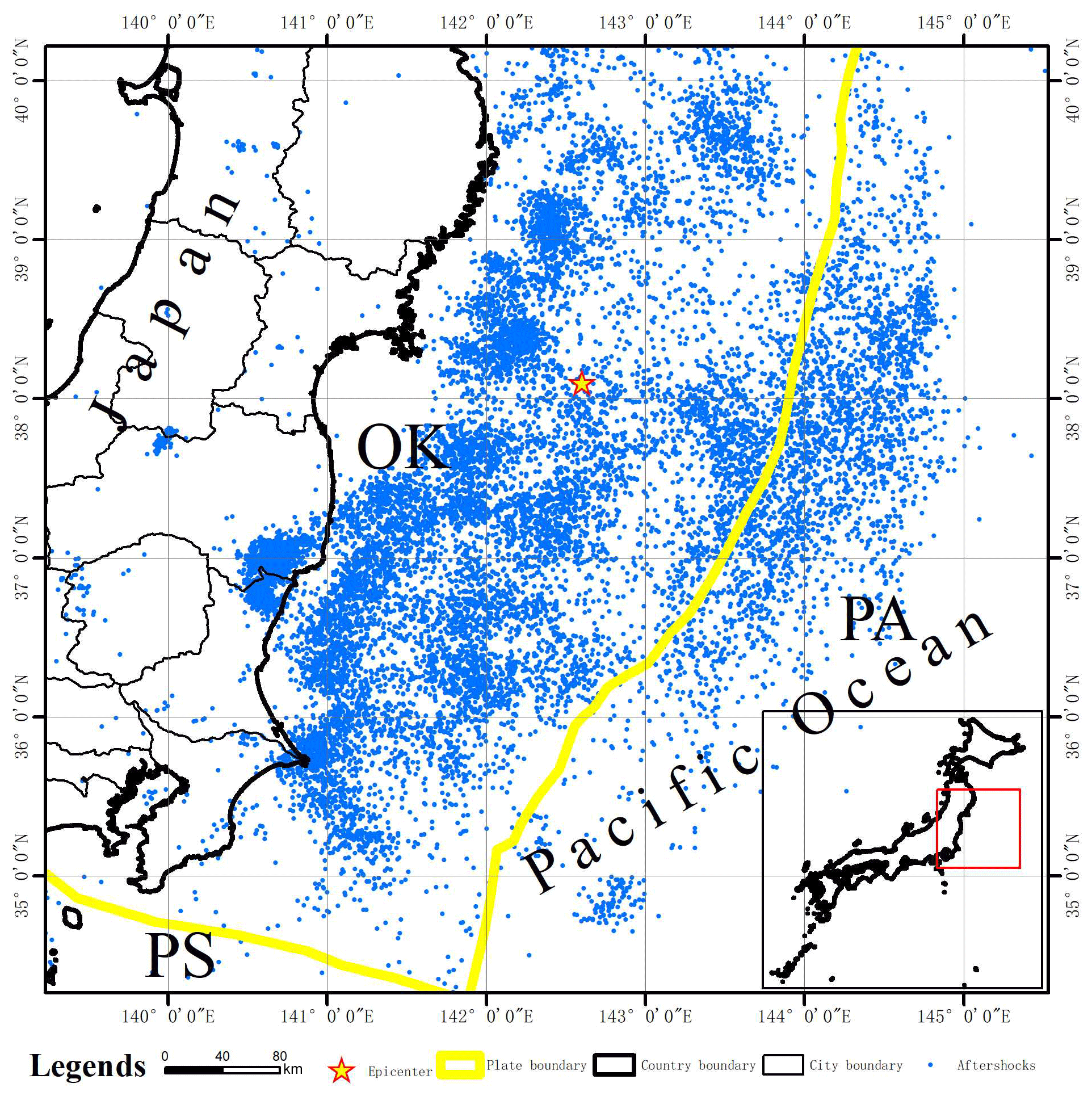
Figure 9 Aftershocks distribution of the Tohoku earthquake. The blue points in the figure are the projection positions of the aftershocks within a depth of 50 km.

3.2 Case selection and data presentation

In order to verify the method and model in this article, we selected two typical historical earthquake cases, i.e., the Wenchuan earthquake and the Tohoku earthquake. These two earthquake cases are not included in the data used for model construction. They are characterized by a large magnitude and a large number of aftershocks.

In the Tohoku earthquake case, there were 15 062 aftershocks in the study area within 1 year after the mainshock (Table 1). In the finite fault model used in this article, the focal depth is 20–25 km, and according to the depth distribution of aftershocks at multiple timescales, the number of aftershocks is the largest at the depth of 35–40 km (Fig. 4a). In the Wenchuan earthquake case, there were 1455 aftershocks in the study area within 1 year after the mainshock (Table 1). In the finite fault model used in this paper, the focal depth is 10–15 km. According to the depth distribution of aftershocks at multiple timescales, the number of aftershocks is the largest at 10–15 km depth. Aftershocks are not necessarily distributed the most on the focal-depth surface (Fig. 4b).

3.3 Application of the model to the Wenchuan earthquake

3.3.1 Aftershock hysteresis failure mode

According to the tectonic stress figure of the Wenchuan earthquake, the Wenchuan earthquake was located in the Longmenshan area in the border mountains east of the Qinghai–Tibetan Plateau. The geological structure in this area is complex. The main Longmenshan fault zone is composed of a series of roughly parallel thrust faults. It is divided into a front mountain zone and a back mountain zone with the Yingxiu–Beichuan central fault as the boundary. From northwest to southeast, the main fault zone consists of the back mountain fault, the central fault and the front mountain fault. The main fault forming the Wenchuan earthquake is the Yingxiu–Beichuan central fault. According to the beach ball plot of the focal-mechanism solution in Fig. 5, the strong aftershocks following the Wenchuan earthquake are mainly related to reverse or thrust faults under the action of compressive stress.

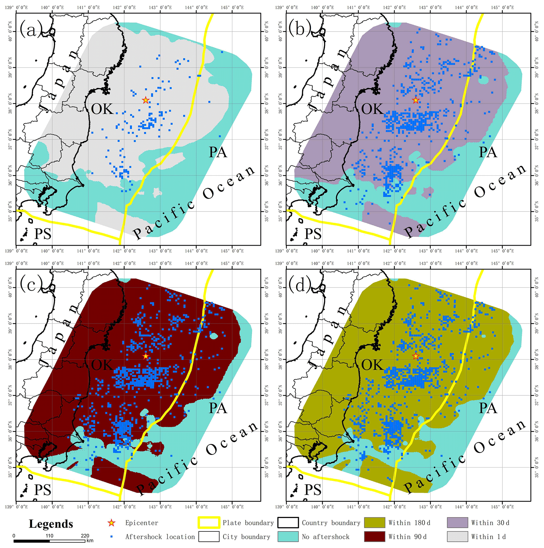
Figure 10 Aftershock damage patterns of the Tohoku earthquake at multiple timescales. Panels (a) through (d) show the aftershock damage pattern of the Tohoku earthquake within 1, 30, 90 and 180 d, respectively. The blue dots indicate the actual location of aftershocks at the corresponding timescale.

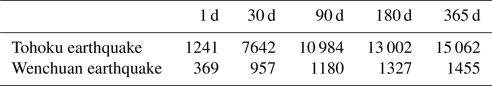
Table 1 The number of aftershocks of typical historical earthquakes on multiple timescales.

Based on the aftershock hysteresis model, the failure patterns of aftershocks are predicted at different timescales, and the section observation is conducted at a depth of 12.5 km (essentially at the same depth as the source). Combined with the focal-mechanism solution analysis of strong aftershocks around the main fault zone, the aftershocks in this area are mainly caused by the NW-trending and SE-trending crustal compressive stress (Fig. 6). The expansion of the aftershock hysteresis pattern is observed, which is generally distributed along the fault strike and extends along the trend line of the main fault. Within 1 d after the main earthquake at Wenchuan, there were aftershocks over a wide area. The location of the aftershocks is distributed along the fault zone, and the location of the aftershocks is basically distributed in the geographical space predicted by the model.

Finally, the spatial results of the hysteresis effect of the Wenchuan earthquake are obtained by synthesizing the damage modes of the aftershocks at multiple timescales (Fig. 7). The location of the aftershocks is basically along the main fault, i.e., the Yingxiu–Beichuan central fault. The model predicts that aftershocks are mainly distributed in the cities of Chengdu, Mianyang, Deyang, Guangyuan and Ngawa, which is consistent with the actual location of the aftershocks. Over time, the area of aftershocks expands outwards, and the rate decreases gradually. Using the main aftershock sequence from the Wenchuan earthquake as an example, the aftershock hysteresis patterns at different timescales are similar, and the direction of outward expansion is basically perpendicular to the distribution direction of the previous timescale. Compared with the attenuation map of earthquake intensity, the spatial distribution map of aftershock attenuation can provide some reference for follow-up disaster prevention and mitigation work after a large earthquake. We can further understand the attenuation law of aftershocks and attempt to extend its time attenuation from a statistical perspective to a spatial perspective.

3.3.2 Aftershock hysteresis patterns at different depths

At different focal depths, the aftershock hysteresis patterns will also change. The focal-depth range of the aftershocks analyzed in this paper is 0–50 km. The aftershock hysteresis effect is analyzed by selecting sections with depths of 2.5, 7.5, 12.5, 17.5, 22.5, 27.5, 32.5, 37.5 and 42.5 km. Many previous studies have shown that the seismogenic layers in central and western China are located in the middle and upper layers of the crust at a depth of no more than 20 km (Zhao and Chen, 1995; Yang et al., 2003). The aftershocks with a focal depth within 20 km are widely distributed (Fig. 8). When the focal depth exceeds 20 km, the area where the aftershocks are generated suddenly decreases with increasing depth until no aftershocks are observed. The focal depth of the largest aftershock distribution range is 12.5 km, which is in the same range as the focal depth of the main earthquake. In the middle and upper layers of the earth's crust, the shapes of the aftershock hysteresis patterns are generally similar at different timescales. Over time, the shape of the aftershock hysteresis pattern generally expands outward in a similar pattern as the previous timescale. However, when the focal depth exceeds a certain value, the hysteresis pattern of the aftershocks substantially changes. In this case, when the focal depth is greater than 20 km, the area predicted for aftershocks significantly decreases, and the evolution of the hysteresis pattern is also changed. Although the overall expansion direction is consistent with the main fault, the pattern is less regular and more random.

3.4 Application of the model to the Tohoku earthquake in 2011

3.4.1 Aftershock hysteresis failure mode

Japan is located in the circum-Pacific seismic belt at the intersection of the Eurasian plate and the Pacific plate, which is an area with a frequent occurrence of global earthquakes. Due to the collision between the Pacific plate and the Eurasian plate, the Pacific plate is subducted under the Eurasian plate, thus forming the Japan Trench and the Japanese island arc. “OK” represents the Okhotsk plate, which is part of the Eurasian plate; “PA” refers to the Pacific plate; and “PS” refers to the Philippine Sea plate, which is also part of the Eurasian plate (Bird, 2003) (Fig. 9). The epicenter of the earthquake was located in the subduction zone of the Japan Trench. The Tohoku earthquake occurred due to the subduction of the Pacific plate to the Eurasian plate. The aftershocks of the Tohoku earthquake mainly occurred near the junction of the Eurasian plate and the Pacific plate. They all belong to the earthquake between the plates. The Japanese offshore plate is mainly the Okhotsk plate, which is part of the Eurasian plate. A total of 12 462 (about 82.7 %) aftershocks occurred in the Okhotsk plate, and 2576 (about 17.1 %) aftershocks occurred in the Pacific plate. Based on the aftershock hysteresis model, the aftershock patterns within 1, 30, 90, 180 and 365 d after the main earthquake are predicted, and the section (22.5 km) at the focal depth of the main earthquake is selected for analysis (Fig. 10). Using the Tohoku earthquake in Japan as an example, the greatest expansion of the aftershock distribution area is observed within 30 d. The shape of the aftershock patterns are similar at all timescales. The aftershock and the predicted aftershock patterns are distributed in an approximately north–south direction along the Japan Trench and plate boundary.

The aftershock hysteresis model of the Tohoku earthquake in is obtained by synthesizing the aftershock patterns at different timescales (Fig. 11). Over time, the expansion rate of the aftershock pattern gradually decreases, and the expansion direction is basically perpendicular to the aftershock pattern at the previous scale. Most of the aftershocks of this earthquake occurred in the eastern Sea of Japan, and the area of concentrated terrestrial aftershocks was located in Fukushima.

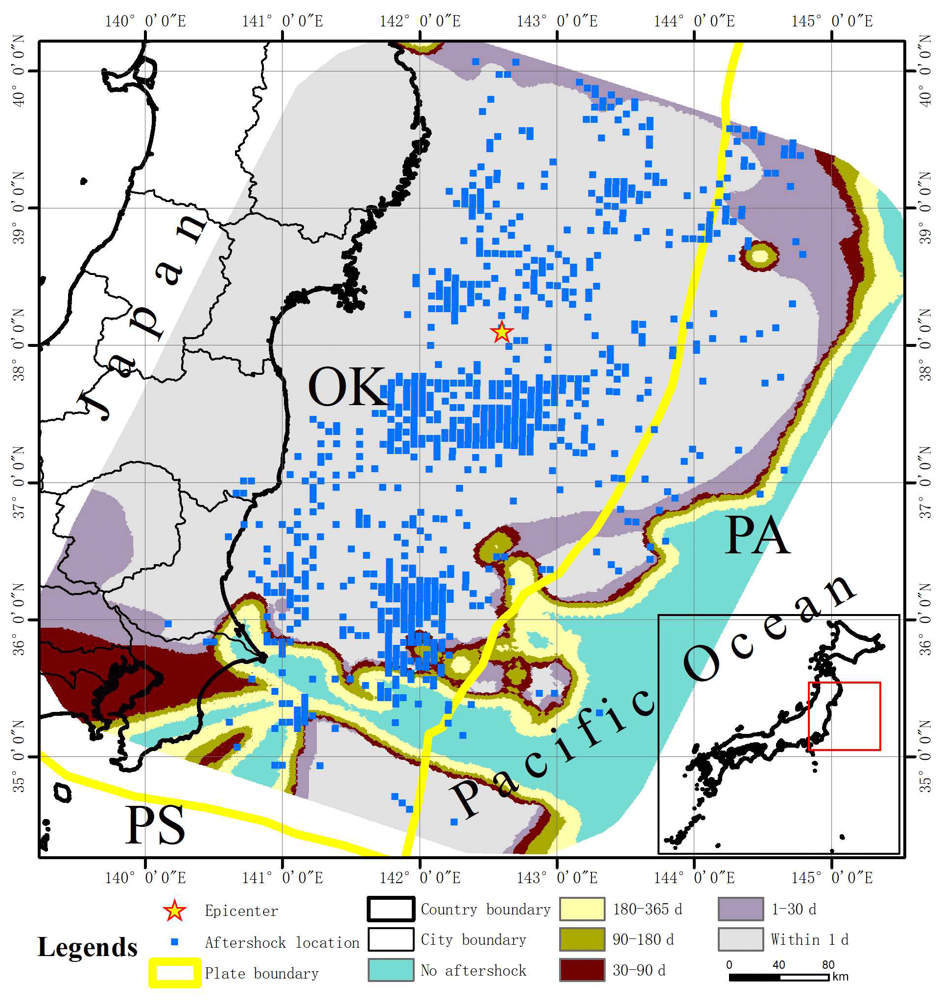
Figure 11 Aftershock hysteresis effect of the Tohoku earthquake in Japan. The aftershock hysteresis effect can be observed by combining the aftershock patterns of the Tohoku earthquake at different timescales. The blue dots indicate the locations of the actual aftershocks over 1 year.

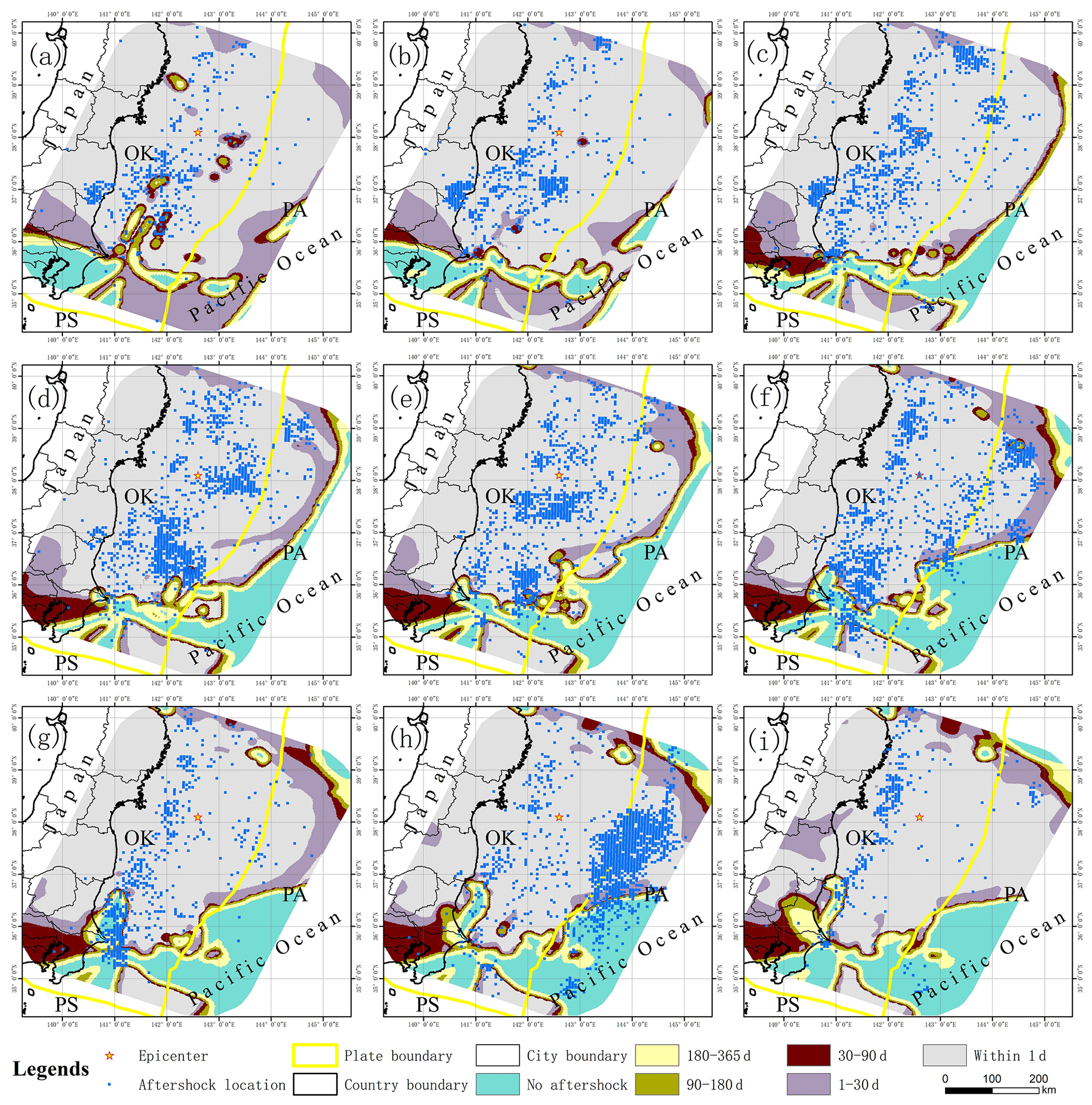
Figure 12 Aftershock hysteresis effect of the Tohoku earthquake at different depths. Panels (a) through (i) show the aftershock hysteresis effect of the Tohoku earthquake for depth sections of 2.5, 7.5, 12.5, 17.5, 22.5, 27.5, 32.5, 37.5 and 42.5 km, respectively.

3.4.2 Aftershock hysteresis patterns at different depths

Similar to the Wenchuan earthquake, the aftershock hysteresis pattern of the Tohoku earthquake changes with the change in depth. The magnitude of the earthquake was very large, reaching over M_w9. The main earthquake has a great impact on the surrounding area, and the crust, which stores considerable energy, then releases it in the form of aftershocks. The predicted expansion direction of the aftershock model is generally consistent with that of the plate boundary and the Japan Trench. In this study, the maximum analysis depth is 50 km. Using the depth section of the mainshock source as the center, the actual aftershock pattern does not change significantly when the depth change is small. This may be due to the large magnitude of the earthquake. The area of the actual aftershock pattern is reduced at a depth of 42.5 km. However, the location of the aftershocks is still widely distributed. The expansion of the aftershock pattern also changes beginning at a depth of 27.5 km. The general direction of distribution is along the trench, and some areas begin to expand vertically along the trench (Fig. 12).

4 Discussion

4.1 Aftershock hysteresis effect

The modified Omori formula is $n\left(t\right)=K(t+c{)}^{-p}$, where n(t) is the aftershock frequency per unit time, and as t increases, n(t) will decrease correspondingly to describe the time attenuation characteristics of aftershocks. In order to analyze the model results better, we use the modified Omori formula to analyze the above two earthquake cases. According to the modified Omori formula, the aftershock attenuation of the two earthquake cases of the Tohoku earthquake and Wenchuan earthquake are analyzed, and the three coefficients in the attenuation formula of the two earthquake cases are determined, namely c, K and p. Based on the modified Omori formula, aftershock attenuation maps of two earthquake cases can be obtained (Figs. 13 and 14). The modified Omori formula reflects the attenuation trend of the occurrence rate of aftershocks over time. The attenuation equations and derivative functions of the two earthquake cases are shown in Table 2. The revised Omori formula can reflect the attenuation of the aftershock event rate over time. In addition, only the quantitative attenuation formula cannot give a good visualization of the attenuation process in space. From the derivative functions of the attenuation formulas of the two earthquake cases, as time increases, the absolute values of the slope of the derivative functions become smaller and smaller. If the aftershock attenuation rate of each earthquake case is calculated on all timescales, it can be found that it gradually decreases as the timescale increases.

Figure 13 The modified Omori formula aftershock attenuation curve of the Tohoku earthquake.

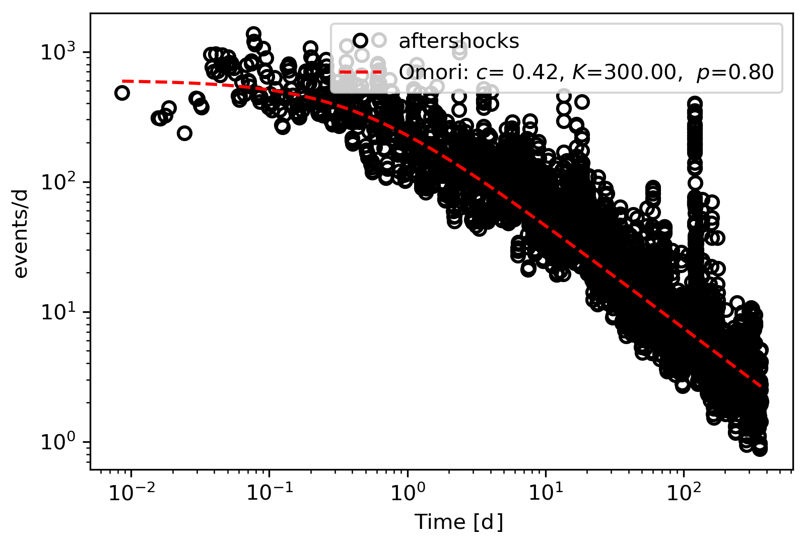
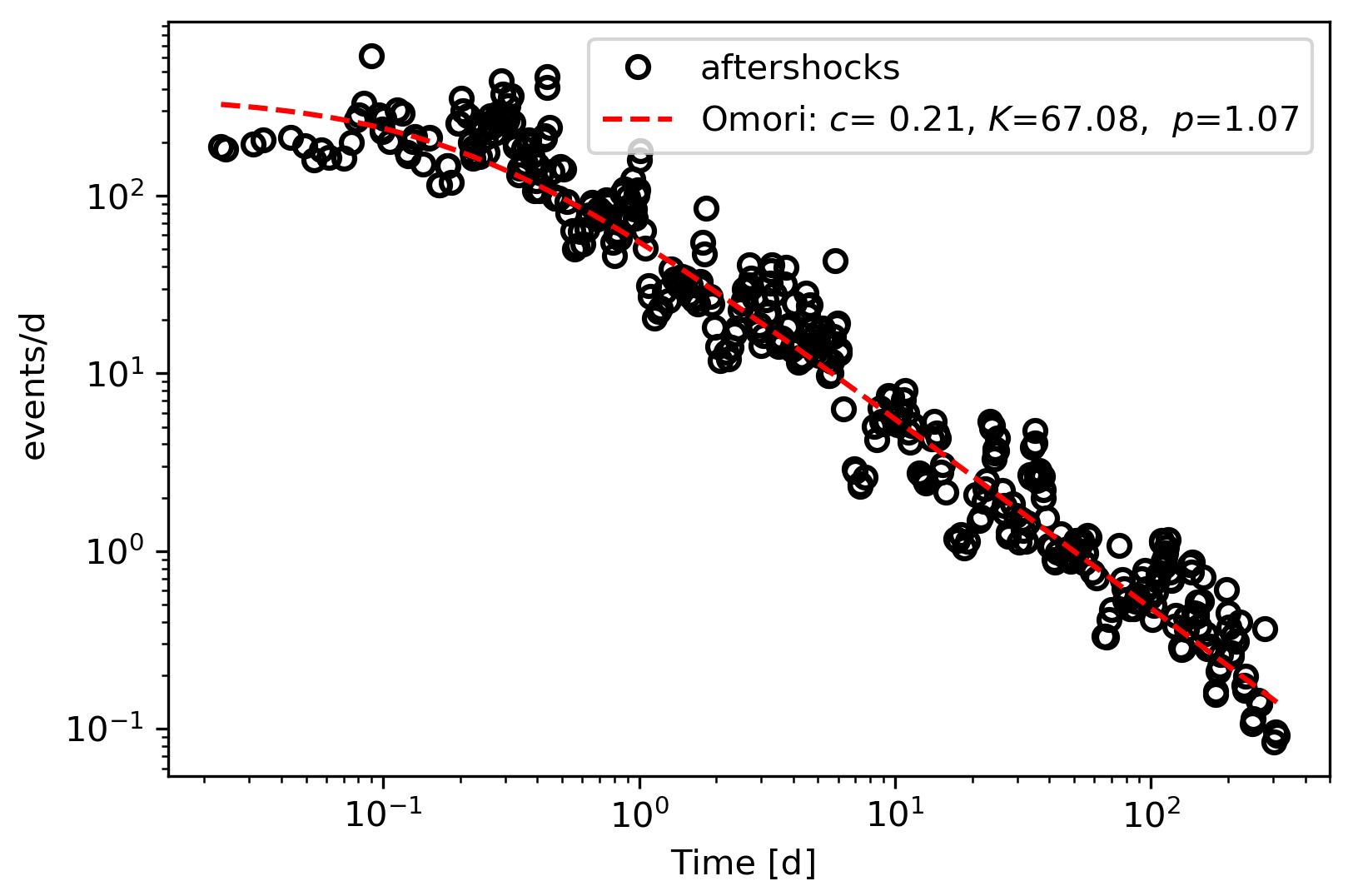
Figure 14 The modified Omori formula aftershock attenuation curve of the Wenchuan earthquake.

Compared with the Omori formula, the aftershock hysteresis effect analyzed in this paper can be reflected by the correlation between the change of timescale and the region of aftershocks. Based on the discussion of focal-depth sections of the main earthquake, within 1 d after the Wenchuan earthquake, the number of subunits with aftershocks is 213; within 30 d, it is 386, representing an increase of 81.6 %; within 90 d, it is 432, representing an increase of 11.9 %; within 180 d, it is 466, representing an increase of 7.9 %; and within 365 d, it is 488, representing an increase of 4.7 %. Within 1 d after the Tohoku earthquake, the number of subunits with aftershocks was 137; within 30 d, it was 595, representing an increase of 334 %; within 90 d, it was 724, representing an increase of 21.7 %; within 180 d, it was 799, representing an increase of 10.4 %; and within 365 d, it was 856, representing an increase of 7.1 %. The aftershock pattern predicted by the model expands over time, but the expansion speed of the aftershock pattern also gradually decreases. The rate of expansion is most rapid 30 d after the earthquake. After 30 d, the speed decreases significantly from 30 to 90 d. The aftershock pattern of the Wenchuan earthquake expanded at a speed of 28.7 units d⁻¹ within 30 d after the earthquake and then rapidly dropped to 7.8 units d⁻¹. The aftershock pattern of the Tohoku earthquake in Japan expanded at a rate of 38.6 units d⁻¹ within 30 d after the earthquake and then dropped rapidly to 7.3 units d⁻¹. According to the correlation curve in Figs. 15 and 16, the aftershock hysteresis effect is reflected by the expansion pattern of the aftershocks. Combined with the comprehensive analysis of the previous two earthquake cases, the expansion rate of the aftershock hysteresis effect is $v\propto n\left(t\right)\propto \frac{\mathrm{1}}{t}$. Unlike previous research on the attenuation law of aftershocks based on statistics (Narteau et al., 2005; Nanjo et al., 2007), this paper starts from another perspective, namely, spatial distribution and returns to the discussion of the attenuation law of aftershock spatial distribution.

Table 2 Modified Omori formula and derived function of typical earthquake cases

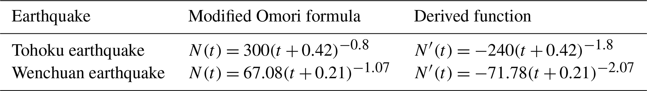
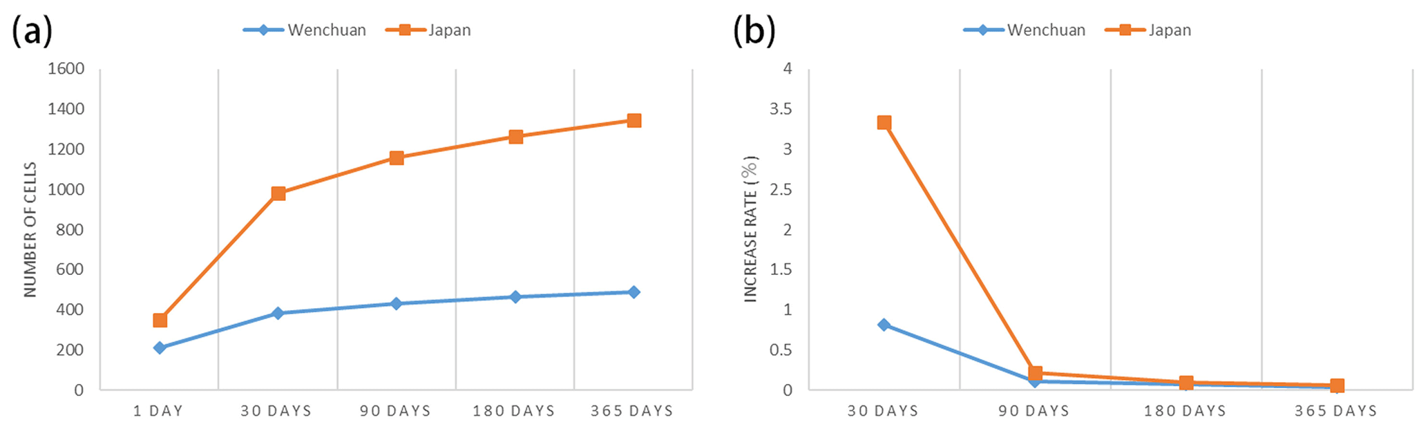
Figure 15 The curve of the aftershock hysteresis effect (actual aftershocks). Panel (a) shows the change in the number of cells with aftershocks at different timescales, and panel (b) shows the change in the growth rate of the number of cells with aftershocks at different timescales.

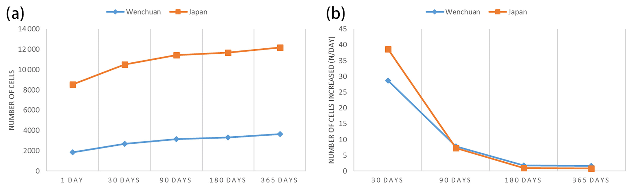
Figure 16 The curve of the aftershock hysteresis effect (predicted aftershock pattern). Panel (a) shows the number of cells with aftershocks predicted at different timescales, and panel (b) shows the increment of cells with aftershocks at each timescale.

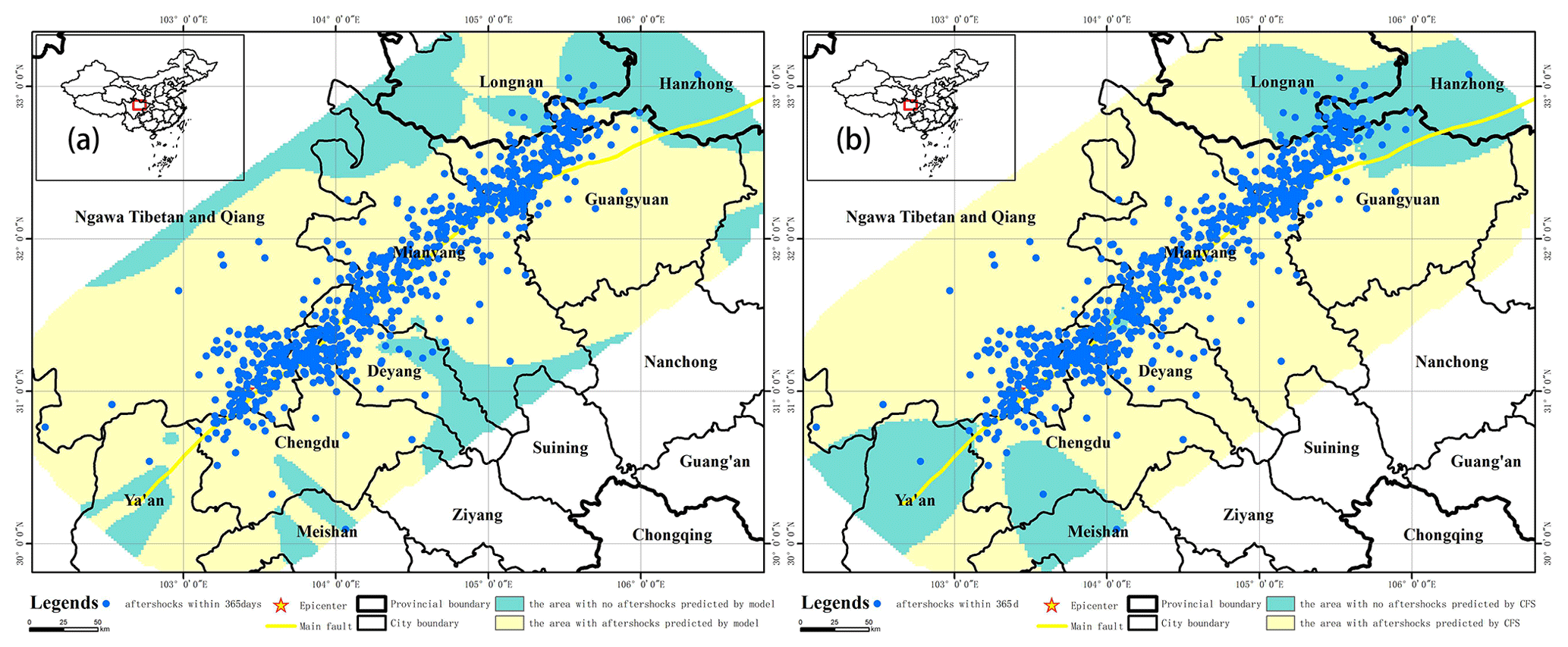
Figure 17 The hysteresis model prediction result and the ΔCFS prediction result of the Wenchuan earthquake. Panel (a) shows the hysteresis model prediction result, and panel (b) shows the ΔCFS prediction result.

Finally, a supplementary explanation is given to the phenomenon that the area predicted by the model is larger than the actual aftershock location. The prediction results of the hysteresis model are the likely locations of aftershocks at different timescales after the mainshock. At each location, the predicted value is a number between 0 and 1, which represents the probability of aftershocks that may occur at that location. We take the prediction threshold as 0.5 and think that when the prediction value is greater than 0.5, an earthquake is more likely to occur in the subcell with a volume of 5 km³. In fact, when the predicted value is less than 0.5, there is also the possibility of aftershocks, but this possibility is relatively small. For the prediction model, if the threshold increases, the predicted coverage area of aftershocks is gradually reduced, but as the increase of threshold, the local area prediction will also produce more errors and deviations. In addition, if we focus on some aftershocks far away from the fault, we will find that aftershocks are also likely to occur at locations far away from the fault on multiple timescales, but the density of aftershocks is relatively small at these locations. Therefore, if these sparsely distributed aftershocks are taken into account, the predicted aftershock coverage area is wider than the area where the aftershocks are concentrated along the fault.

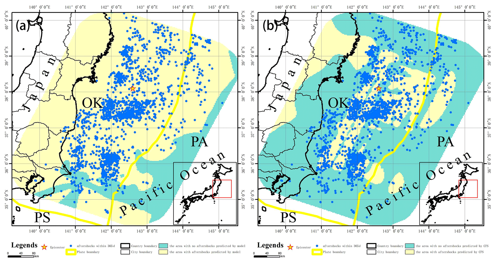
Figure 18 The hysteresis model prediction result and the ΔCFS prediction result of the Tohoku earthquake. Panel (a) shows the hysteresis model prediction result, and panel (b) shows the ΔCFS prediction result.

4.2 Comparative analysis of prediction models

The widely used temporal-magnitude earthquake generation model (ETAS) was proposed by Ogata (Ogata, 1988). Later on, he observed that the distribution of aftershock sequences tended to be elliptic rather than circular. He established the anisotropic aftershock attenuation function and took the normal distribution as the spatial distribution model of an aftershock (Ogata, 1998). It is a widely observed fact that aftershocks usually occur on or near the fault of a mainshock. However, the normal distribution model does not include the source mechanism information of the mainshock when predicting the aftershock mode. Kagan et al. introduced the anisotropy function of the spatial smooth core into long-term earthquake prediction and established the spatial-smooth-core model, including the source mechanism information of the mainshock (Kagan and Jackson, 1994). However, the above models ignore the internal relationship of the relative distance or direction between the mainshock and the aftershocks. Based on this, Wong and Schoenberg (2009) proposed a joint distribution model to parameterize the aftershock location according to the distance and relative angle between the mainshock and aftershocks (Wong and Schoenberg, 2009). In the prediction process of the above models, the epicenter of the mainshock is used as a point source for analysis. Actually, the distribution of the fault plane of the mainshock should be fully considered. Based on the finite fault model, the distribution information of the main fault is considered in the paper. At the same time, the relative position and direction between the mainshock and aftershocks have been considered in the process of calculating the variation of stress tensor by using the Okada dislocation theory. Therefore, in the process of model training and learning, the relative-position relation is also identified. Compared with the static Coulomb failure stress change method, the aftershock hysteresis model has a better prediction effect.

In the previous comparison of the two methods in this article, the subcell location where the aftershock was located was used for evaluation, and the subcells with aftershocks were marked. To further prove the validity of the model, the actual location of the aftershock event is further used instead of the subcell location, and the threshold is set to 0.5. The prediction results were verified on the focal depth of the two earthquake cases to compare the effects of the aftershock hysteresis model and the Coulomb failure stress change method. The evaluation results of the aftershock hysteresis model are as follows: 97.6 % of the Wenchuan earthquake aftershocks fall in the area with the predicted value greater than 0.5, and 96 % of the Tohoku earthquake aftershocks fall within the area with the predicted value greater than 0.5. The evaluation results based on the Coulomb failure stress change method are as follows: 87.3 % of the Wenchuan earthquake aftershocks fall in the area with a predicted value greater than 0.5, and 45.3 % of the Tohoku earthquake aftershocks fall within the area with a predicted value greater than 0.5 (Figs. 17 and 18). Therefore, if the evaluation is made from the specific location of the aftershock event, the prediction result of the constructed model is still better than the result based on the Coulomb failure stress change method.

In addition, the model is a six-layer neural network, which is a black box model. Compared with the traditional statistical model or physical model, is the deep learning model more complex? We think this complexity is relative. In fact, the starting point of the traditional model and of the model in this paper are similar. They are all based on data, trying to find a relationship between some basic physical quantities and aftershocks. The complexity of traditional models lies in the process of finding such a connection. The complexity of the deep learning model lies in its seemingly complex structure. The complex structure will lead to the increase of the number of internal variables to be learned, and the rapid computing ability of today's computers can solve this problem, thus reducing man power and time-consuming work. In addition, the deep learning model is a data-driven method. It will be more convenient than the traditional model when the dataset or the amount of data changes greatly or the model needs to be adjusted.

5 Conclusions

In this paper, based on the criterion of correlation between aftershocks and stress changes caused by the main earthquakes, a deep neural network is trained using the SRCMOD finite fault data and the ISC earthquake catalogue and is used to construct an aftershock hysteresis model. Using the main aftershock sequences of the Wenchuan and the Tohoku earthquakes as examples, the characteristics of the aftershock hysteresis effect in plane space and at different depths are then analyzed. The main contributions are as follows:

1. The trained model of aftershock hysteresis is accurate. It can predict the aftershock patterns at multiple timescales after a large earthquake and produce a spatial distribution map of the aftershock hysteresis effect. Compared with static Coulomb failure stress change, this model is more effective.

2. Compared with the traditional aftershock spatial analysis method, the model fully considers the distribution of actual faults in the prediction of an aftershock pattern, instead of treating the earthquake as a point source. In the analysis of the model, the relative-position information between the mainshock and aftershocks has been included.

3. The expansion rate of the aftershock patterns changes over time, i.e., $v\propto n\left(t\right)\propto \frac{\mathrm{1}}{t}$. In the middle and upper layers of the crust, the shape of the aftershock pattern is generally consistent, and the expansion direction is typically perpendicular to the direction of distribution of the previous timescale.

4. According to the prediction results of the model, the aftershock patterns at all timescales are roughly similar and anisotropic. The distribution law of aftershock hysteresis effect will change with the increase of the depth.

In the analysis of each aftershock sequence, we only consider the influence of the main earthquake fault zone. If we comprehensively consider the stress field superposition of multiple or all faults in the analysis area of each earthquake case, the prediction of the aftershock pattern will be more accurate. In addition, we focus on the location of the aftershocks and will further explore and study aftershocks from the perspectives of magnitude and energy in the future.