The contribution of air temperature and ozone to mortality rates during hot weather episodes in eight German cities during the years 2000 and 2017

Hot weather episodes are globally associated with excess mortality rates. Elevated ozone concentrations occurring simultaneously also contribute to excess mortality rates during these episodes. However, the relative importance of both stressors for excess mortality rates is not yet known and assumed to vary from region to region.

This study analyzes time series of daily observational data of air temperature and ozone concentrations for eight of the largest German cities during the years 2000 and 2017 with respect to the relative importance of both stressors for excess mortality rates in each city. By using an event-based risk approach, various thresholds for air temperature were explored for each city to detect hot weather episodes that are statistically associated with excess mortality rates. Multiple linear regressions were then calculated to investigate the relative contribution of variations in air temperature and ozone concentrations to the explained variance in mortality rates during these episodes, including the interaction of both predictors.

In all cities hot weather episodes were detected that are related to excess mortality rates. Across the cities, a strong increase of this relation was observed around the 95th percentile of each city-specific air temperature distribution. Elevated ozone concentrations during hot weather episodes are also related to excess mortality rates in all cities. In general, the relative contribution of elevated ozone concentrations on mortality rates declines with increasing air temperature thresholds and occurs mainly as a statistically inseparable part of the air temperature impact. The specific strength of the impact of both stressors varies across the investigated cities. City-specific drivers such as background climate and vulnerability of the city population might lead to these differences and could be the subject of further research.

These results underline strong regional differences in the importance of both stressors during hot weather episodes and could thus help in the development of city-specific heat–ozone–health warning systems to account for city-specific features.

1 Introduction

Hot weather episodes (HWEs) cause more human fatalities in Europe than any other natural hazard (EEA, 2019a). HWEs are typically characterized by elevated air temperature and can last for several days or weeks, depending on the respective threshold values that are used to identify such days. Numerous investigations found excess mortality rates during days of elevated air temperature (Curriero et al., 2002; Anderson and Bell, 2009; Gasparrini and Armstrong, 2011; Gasparrini et al., 2015). Increases in morbidity rates, hospital admissions and emergency calls are also associated with elevated air temperatures (Bassil et al., 2009; Karlsson and Ziebarth, 2018). In addition, HWEs are linked to increased tropospheric ozone concentrations (Shen et al., 2016; Schnell and Prather, 2017; Phalitnonkiat et al., 2018). Zhang et al. (2017) and Schnell and Prather (2017), for example, found for North America that the probability is up to 50 % that both air temperature and ozone concentrations reach their 95th percentile simultaneously. Ozone as a secondary air pollutant is formed by photochemical reactions of volatile organic compounds and nitrogen oxides. Increased air temperature and high solar radiation intensify this formation (Camalier et al., 2007; Varotsos et al., 2019). Correlations between both environmental stressors are mostly described as linear (Steiner et al., 2010). A variety of geographic and meteorological factors may influence this relationship, such as the presence of precursors, local-specific wind patterns or the humidity content of the lower atmosphere (Steiner et al., 2010). At the upper end of the respective air temperature and ozone concentration distributions, the direct linkage between the two stressors is discussed to be even more complex (Steiner et al., 2010; Shen et al., 2016). Despite this linkage, elevated ozone concentrations alone have also been associated with adverse health effects (Bell, 2004; Hůnová et al., 2013; Bae et al., 2015; Díaz et al., 2018; Vicedo-Cabrera et al., 2020). The close linkage of both environmental stressors makes it necessary to account for their confounding influence on each other, in order to investigate distinctive health effects of each of these two stressors. But beyond the consideration of both environmental stressors as separated elements, their co-occurrence may lead to even higher rates of excess mortality (Burkart et al., 2013; Vanos et al., 2015; Scortichini et al., 2018; Krug et al., 2019). Some studies also indicate an interactive effect, which is larger than the sum of their individual effects (Cheng and Kan, 2012; Burkart et al., 2013; Analitis et al., 2018).

Studies which investigate regional differences in the relation between HWEs and ozone concentrations revealed differences in the air-temperature–ozone relationship (e.g., Shen et al., 2016; Schnell and Prather, 2017; Phalitnonkiat et al., 2018) and in terms of their individual and combined effects on mortality (Filleul et al., 2006; Burkart et al., 2013; Analitis et al., 2014; Breitner et al., 2014; Tong et al., 2015; Analitis et al., 2018; Scortichini et al., 2018). Some studies report a north–south gradient in the air-temperature–mortality relationship, indicating that populations of northern regions are more sensitive to heat compared to southern regions, which are more affected by cold (e.g., Burkart et al., 2013; Scortichini et al., 2018). However, the influencing effect of elevated ozone concentrations is shown to be more differentiated. While some studies report a greater influence of elevated ozone concentrations for more heat-affected regions (Anderson and Bell, 2011; Scortichini et al., 2018), other studies discuss that regional differences are a result of location-specific physiological, behavioral and socio-economic characteristics, as well as the specific level of exposure across various cities (Anderson and Bell, 2009, 2011; Burkart et al., 2013; Breitner et al., 2014). For Germany, most studies investigated the effect of air temperature during HWEs on mortality for different regions (Gabriel and Endlicher, 2011; Scherer et al., 2013; Muthers et al., 2017; an der Heiden et al., 2019). Breitner et al. (2014) investigated short-term effects of air temperature on mortality and modifications by ozone in three cities in southern Germany. But, to our knowledge, a national multi-city study exploring the impacts of HWEs on mortality across different German cities has not been carried out so far. In addition, how ozone concentrations contribute to mortality rates during HWEs is inconclusive for different cities in Germany and worldwide, as described above.

A prior study for Berlin, Germany (Krug et al., 2019), identified HWEs and episodes of elevated ozone concentrations with a risk-based approach for the period 2000 to 2014. Whereas ozone concentrations alone only showed a weak relationship to mortality rates, the co-occurrence with elevated air temperatures amplified mortality rates in Berlin. On the basis of these results, the main focus of this study lies in the identification of HWEs in multiple cities in Germany and the investigation of how air temperature and ozone concentrations contribute to mortality rates during these episodes. Furthermore, the analysis period is extended up until 2017.

The main goals of this study are (a) to identify HWEs that show statistical relations to mortality rates for eight of the largest German cities and (b) to compare these cities in terms of their location-specific relation of air temperature and ozone concentrations to mortality rates. This study is structured by the following research questions:

1. Do other German cities, similar to Berlin, show a significant relationship between HWEs and their specific mortality rates?

2. How does this relationship differ in terms of city-specific threshold values and the relative contribution of air temperature and ozone concentrations during HWEs to the overall explained variance of the mortality rate?

2 Data and methods

2.1 Data

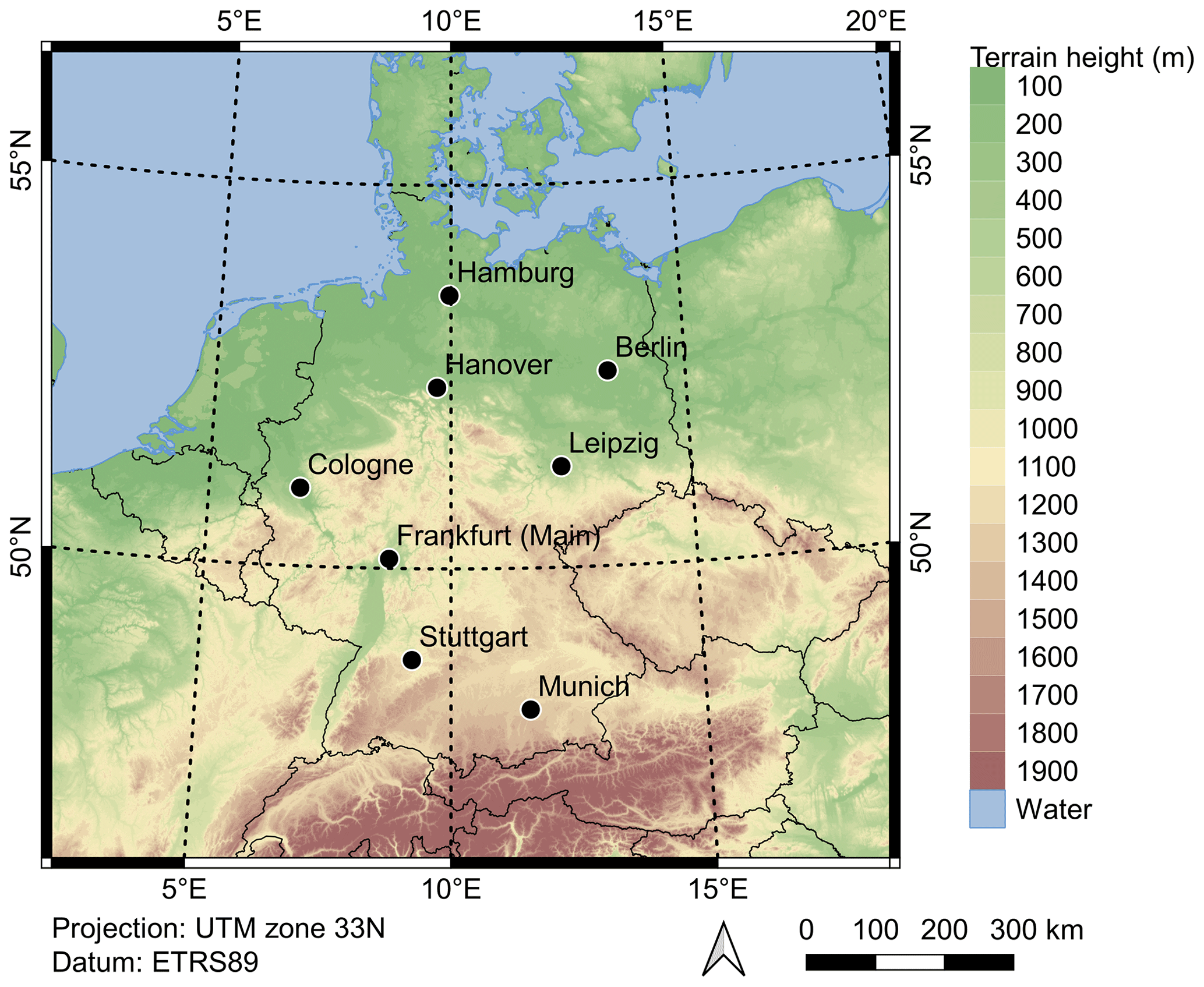
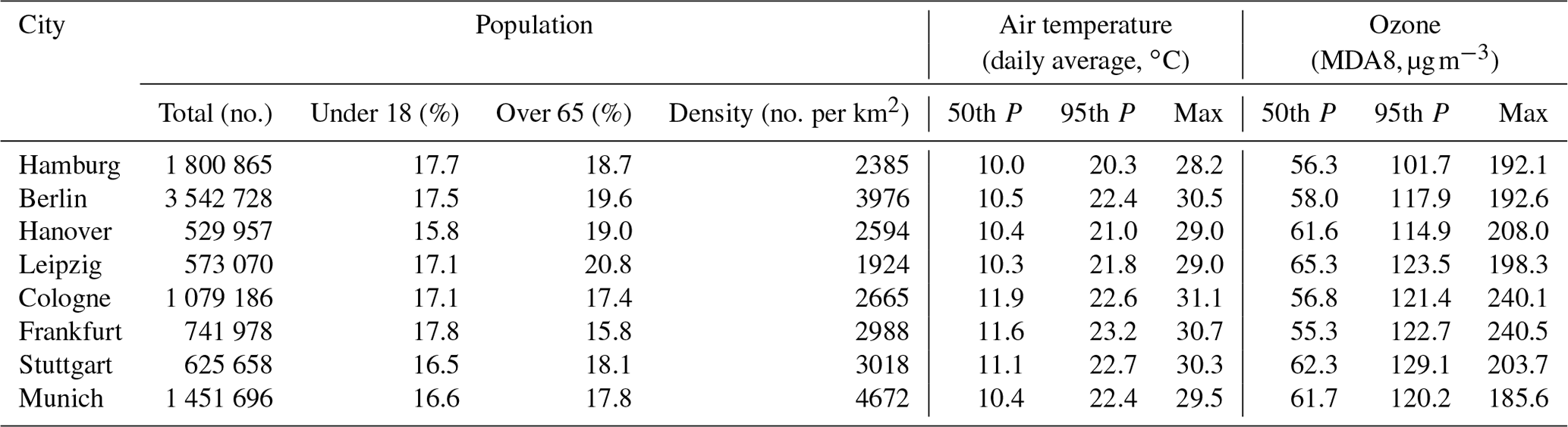
The period analyzed in this study is the 18 years from 2000 to 2017. Eight cities are investigated (in the order of their population): Berlin, Hamburg, Munich, Cologne, Frankfurt (Main), Stuttgart, Leipzig and Hanover (Fig. 1, Table 1). While the first six are the six most populous cities in Germany, the latter two were included in this study to ensure a spatially relatively homogeneous distribution of the investigated cities in Germany. The analyzed cities comprised 10.3 million inhabitants at the end of 2017, which was 12.5 % of the entire German population at this time (DESTATIS, 2019). The smallest city in terms of population (Hanover) has > 500 000 inhabitants, while the largest (Berlin) has > 3.5 million (Table 1).

Figure 1 Location of investigated cites. Topographic map is based on GTOPO30 data retrieved from European Environment Agency (EEA, 2016).

2.1.1 Air temperature

Air temperature data at daily resolution were obtained from the German Weather Service (DWD, 2019). The selection of measurement sites was based on the availability of data covering the entire analysis period. For cities with more than one measurement site, the site closest to the city center and to the co-located ozone measurement site was selected. An overview of the selected measurement sites including their metadata is given in Table A1 and Fig. A1 in the Appendix. We tested daily minimum (TN), maximum (TX) and average air temperature (TA) from each station as predictor variables for mortality rates. The results for all investigated cities are displayed in Fig. A2 in the Appendix. Considering all cities and thresholds, TN and TA performed better than TX. This confirms results of previous studies that found TA to be a suitable predictor for the air-temperature–mortality relationship and a suitable indicator for the city's diurnal thermal conditions, compared to TX or TN (Hajat et al., 2006; Anderson and Bell, 2009; Vaneckova et al., 2011; Yu et al., 2010; Scherer et al., 2013; Chen et al., 2015).

2.1.2 Ozone concentrations

Data of hourly ozone concentrations were obtained from the German Environment Agency (UBA). These data stem from the air quality monitoring networks of the German federal states. To select one ozone monitoring station per city, the same criteria as for the selection of TA measurement sites were applied (closest to city center and to TA site). Only “urban background” stations were selected, as the ozone concentrations should be “representative of the exposure of the general urban population” (EU, 2008). The daily maximum 8 h moving average (MDA8) was calculated from hourly values for all selected sites, which is the widely used metric for ozone monitoring for human health purposes (WHO, 2006; EU, 2008).

2.1.3 Population data

Time series of annual population counts were obtained for each city from the German Federal Bureau of Statistics (DESTATIS, 2019). The German census of 2011 revealed an error between 1 % and 5 % to the previously available annually updated version of the population time series for the selected cities, based on the prior census in 1990. Therefore, population time series were corrected based on the assumption that the error (a) increases over time and (b) correlates with the strength of the annual migration of each city. An error term was calculated for each year of the census period from 1990 to 2010 as the annual proportion of the total error (derived from the difference in the two census data in 2011). Each error term was further weighted by the proportion of the annual migration size from total migration size during the census period. This weighted error term was then subtracted from the annual population size. Years 2012 to 2017 were likewise corrected based on aforementioned assumptions. Annual time series were then linearly interpolated to daily values for each city.

2.1.4 Mortality data

Daily values of deaths for each city were provided by the German Federal Bureau of Statistics (DESTATIS, 2019). We intentionally consider all-cause and all-age total death counts of the whole city in this study, as the main goal is to explore the process which could have an effect (e.g., mortality) as a city-wide variable without any pre-assumption of disease-specific and heat-related health effects. For that reason, we do not want to exclude any death counts from the analysis that might be related to TA or MDA8. Mortality rates were calculated by dividing daily death counts by daily interpolated population counts.

Each time series of TA, MDA8, population and mortality rate were tested for a long-term annual trend. Whereas for TA and MDA8 no significant long-term trend could be detected over the analysis period, mortality rates in all cities showed a significant (p< 0.05, double-sided t test) negative annual trend. This trend was corrected for to avoid any misinterpretation of the variance in the time series.

2.2 Methods

The methodological approach used in this study follows the concept of risk evaluation by the Intergovernmental Panel on Climate Change (IPCC) (IPCC, 2012). This concept was adopted for an explorative event-based risk analysis, which is explained in detail by Scherer et al. (2013) and used in previous works to deduce two risk-based definitions of heat waves (Fenner et al., 2019) or to quantify heat-related risks and hazards (Jänicke et al., 2018). This approach was also used to analyze the co-occurrence of HWEs and episodes of elevated ozone concentrations in Berlin (Krug et al., 2019). The main advantage of this approach is that it explores time series without any pre-assumptions concerning threshold value, length or existing relation between potentially hazardous episodes (here described with TA) and an effect variable (here the mortality rate). In order to identify HWEs with a significant relation to mortality rates, the approach as described in Krug et al. (2019) was applied. In that prior study, time series of TA and MDA8 were explored separately and the episodes, described as “events”, were afterwards classified as temporally separated or co-occurring events of elevated TA and MDA8. Deviating from that approach, only HWEs as characterized by elevated TA and identified by various threshold values are analyzed in this study. MDA8 is treated as an additional stressor during HWEs and analyzed as described in Sect. 2.2.2.

2.2.1 Detection of HWEs

Time series of TA for each city were searched for HWEs as the occurrence of at least three consecutive days exceeding a certain TA threshold value (TA_Thres). TA_Thres was iteratively increased in 0.5 ^∘C steps within the range 10 to 30 ^∘C. Secondly, at each TA_Thres TA magnitude (TA_Mag) was calculated for each HWE as the accumulated sum of the difference of daily TA and respective TA_Thres over the whole length of the HWE (sum of degree days above TA_Thres). Thirdly, univariate linear regressions were calculated between TA_Mag as predictor variable (logarithmized) and mean mortality rates during the HWE plus a maximum number of lag days (to account for possible lag effects in mortality rates after HWEs) as the dependent variable over the whole study period. Regression models thus consist of a unique combination of TA_Thres and maximum lag days. Models for each TA_Thres were tested for a lag effect of maximum 0 to 7 d. Afterwards, the lag effect was fixed to 4 d, which was the mean lag effect across the analyzed cities. All presented results are based on this number (four). Episode-specific mean mortality rates of each model were tested for normal distribution (not shown). Results indicate inconclusive findings of normal and significant non-normal tested distributions dependent on city and model-specific TA_Thres. In conclusion, we keep the assumption of a quasi-normal distribution of mean mortality rates during HWEs, acknowledging that our method is not the one ideal approach, or better than others, for any investigations using mortality data. However, in terms of our research questions it delivers sufficient information about detection and characterization of HWEs as aimed in this study. The base mortality rate for each model is provided as the mortality rate for zero TA_Mag (y intercept of the regression model), indicating conditions of no thermal stress. This approach was also sensitivity-tested for seasonal variances in the mortality rate by the use of a seasonal de-trended, LOESS-smoothed (Cleveland, 1979) mortality time series instead of the crude mortality rate. Differences are negligible, which shows that the original approach chosen is insensitive to seasonal variances. In addition, HWEs occur usually during summer months when mortality rates are low. For each regression model, the explained variance (r²) was calculated. Error probabilities were calculated with a double-sided t test. Regression models which were not statistically significant (p> 0.05) or comprised fewer than five HWEs over the study period were discarded from further analyses. Error estimates for each regression model were calculated as the standard error of the regression coefficient (RE_RC) and of the base mortality rate (RE_BR). Regressions were also calculated for HWEs with a minimum duration of consecutive days different from three (1 to 5 d). The chosen minimum duration of three days yielded best results in terms of r², RE_BR and RE_RC.

2.2.2 Multiple linear regressions

After detection of HWEs, mean MDA8 (MDA8_M) values were calculated for the total duration of each HWE. Multiple linear regressions (MLRs) were then calculated using the ordinary least square error method with TA_Mag and MDA8_M of each HWE as predictor variables for mean mortality rates (as described in Sect. 2.2.1). The overall explained variance (r²) and adjusted explained variance ($r_{\mathrm{adj}}^{\mathrm{2}}$) as well as the explained variance for each single variable ($r_{{\text{TA}}_{\text{Mag}}}^{\mathrm{2}}$ and $r_{{\text{MDA8}}_{\text{M}}}^{\mathrm{2}}$) were calculated. An interaction term ($r_{{\text{TA}}_{\text{Mag}},{\text{MDA8}}_{\text{M}}}^{\mathrm{2}}$) was also estimated as a cross-product effect of both predictor variables. Overall statistical significance is assumed for an error probability of p< 0.05, calculated with a F test.

3 Results

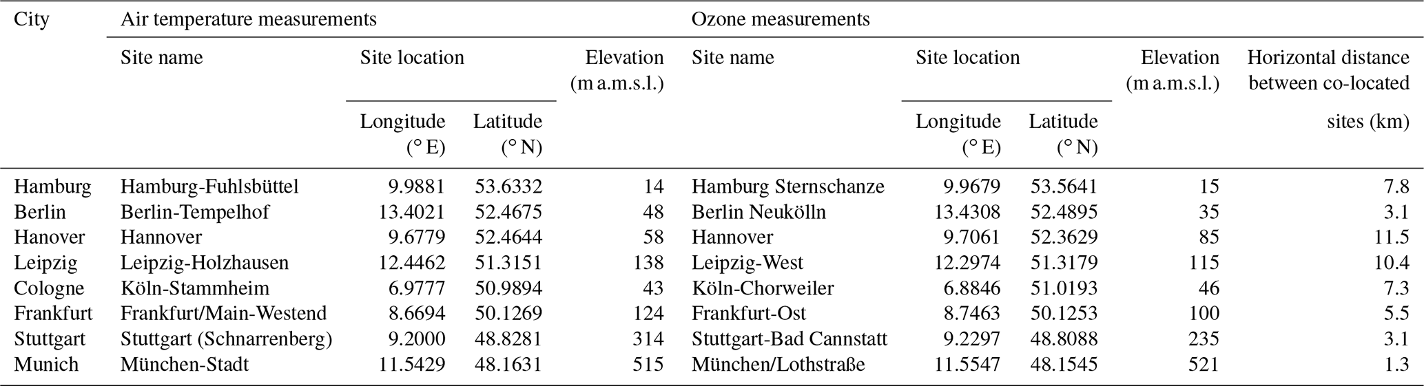
Table 1 shows statistics for TA and MDA8 during the analysis period for each city. The 50th percentile of TA ranges from 10.0 ^∘C in Hamburg to 11.9 ^∘C in Cologne. For the analyzed cities, the highest recorded maximum TA is 31.1 ^∘C in Cologne and the lowest 28.2 ^∘C in Hamburg. The 50th percentile of the MDA8 concentration varies between 55.3 µg m⁻³ in Frankfurt and 65.3 µg m⁻³ in Leipzig. In two cities, Frankfurt and Cologne, by far the absolute highest MDA8 concentrations were recorded during the study period (> 240 µg m⁻³, Table 1).

Table 1 Overview of city-specific statistics of the population (census corrected) on 31 December 2017. Statistics of air temperature and ozone concentrations are based on data from selected measurement sites during the years 2000 to 2017 (Table A1, Fig. A1). Cities are sorted from north to south; P refers to percentile. Sources are as follows: population data from DESTATIS (2019), air temperature from DWD (2019), and ozone concentrations from the German Environment Agency (UBA), based on original data from air quality monitoring networks of the German federal states.

3.1 Regression analysis

Figure 2 presents results of the univariate regression analysis. For all cities, the analysis yields statistically significant results between TA_Mag and mean mortality rates during HWEs for a variety of TA_Thres. In all cities, statistically significant models are characterized by a minimum absolute TA_Thres between 16 and 18 ^∘C (Fig. 2, left panel). Results of all cities show generally increasing r² with increasing TA_Thres. Yet, differences across cities can be seen in the range of TA_Thres and r² of the regression models. The highest values for r² are obtained for Berlin, Cologne, Frankfurt and Stuttgart with values of more than 60 % for HWEs of high TA_Thres. Cities with generally high TA (Table 1) also yield the highest values of r². This may be a result of the absence of HWEs identified by higher TA_Thres in cities like Hamburg, Hanover, Leipzig and Munich compared to the others. For all cities, increased mortality rates during HWEs with TA_Thres ≤ 22 ^∘C can be explained by around 20 % of TA_Mag. Values of RE_BR are low for each city (< 0.2) but show an increase towards higher TA_Thres. Values of RE_RC are heterogeneous across different models as well as across different cities.

Whereas the range of absolute TA_Thres of significant models varies across the cities, a percentile-based order reveals a more similar pattern in terms of threshold–r² relationship across the cities (Fig. 2, right panel). For HWEs with TA_Thres > 95th percentile of the year-round TA distribution in 2000 to 2017, at least 20 % of the mortality rate can be explained by TA_Mag across all cities. An increase in r² can be observed for all cities for HWEs with TA_Thres > 94th percentile.

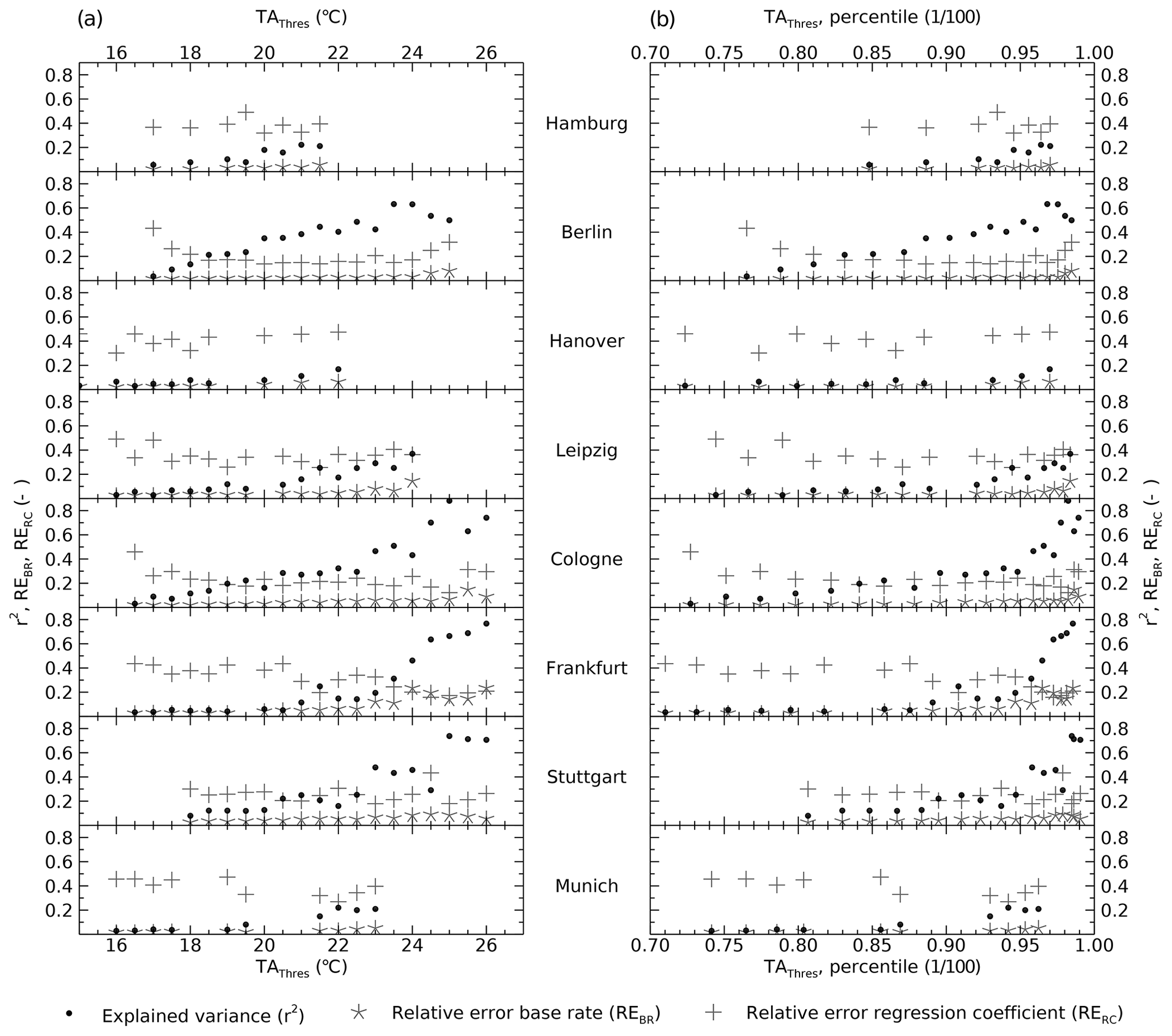
Figure 2 Statistically significant results (p< 0.05, t test) from the univariate regression analysis with TA_Mag as predictor variable for each city: (a) x axis: absolute threshold value for HWE detection (TA_Thres) and (b) x axis: percentile of TA_Thres referring to the whole analysis period 2000 to 2017. y axis: explained variance of the models (r²), relative errors of the base rate (RE_BR) and the regression coefficient (RE_RC), respectively.

3.2 Multiple linear regression analysis

Results of the multiple linear regression and partitioning of r² are shown in Fig. 3. Generally, the highest values are obtained for $r_{{\text{TA}}_{\text{Mag}}}^{\mathrm{2}}$, increasing with increasing TA_Thres. This can be observed for almost all cities, while $r_{{\text{TA}}_{\text{Mag}}}^{\mathrm{2}}$ values vary between cities. In particular, for HWEs identified by higher TA_Thres values, variance in TA_Mag alone explains at least 20 % up to 60 % of the mortality rates in Berlin, Cologne, Frankfurt and Stuttgart. Other cities show overall lower values of $r_{{\text{TA}}_{\text{Mag}}}^{\mathrm{2}}$. Results also reveal that in all cities the variance of mortality rates during these HWEs can partly be explained by the variance of MDA8_M, independently of TA_Mag. Particularly in Berlin, but also in Hanover and Stuttgart, mortality rates during HWEs identified by high TA_Thres cannot solely be explained by MDA8_M. However, this does not apply to Frankfurt, where $r_{{\text{MDA8}}_{\text{M}}}^{\mathrm{2}}$ values reach higher values compared to $r_{{\text{TA}}_{\text{Mag}}}^{\mathrm{2}}$ and, in addition, increase with increasing TA_Thres (Fig. 3f). Differences between cities are also observable for the interaction term between both variables ($r_{{\text{TA}}_{\text{Mag}},{\text{MDA8}}_{\text{M}}}^{\mathrm{2}}$). Whereas some cities show only marginal values (Hamburg, Hanover, Munich), the others show an increasing interaction term with increasing TA_Thres, reaching up to 60 % in Frankfurt. A different pattern for the interaction term is visible for Berlin. The highest values of $r_{{\text{TA}}_{\text{Mag}},{\text{MDA8}}_{\text{M}}}^{\mathrm{2}}$ are obtained for medium TA_Thres with declining trend towards higher TA_Thres.

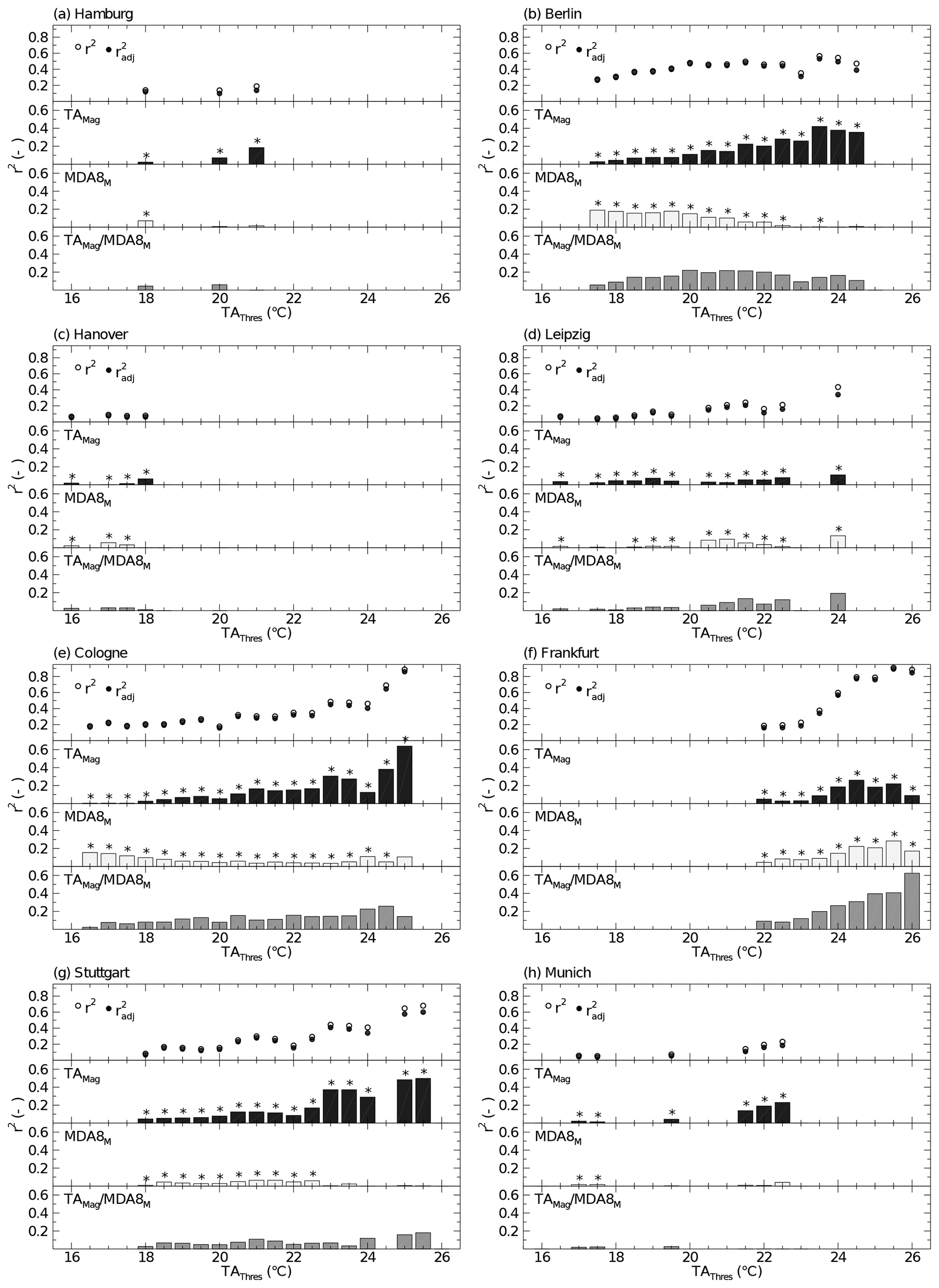
Figure 3 Results of the multiple linear regression (MLR) analysis between the predictor variables TA_Mag and MDA8_M and the mean mortality rate during HWEs as an independent variable. Each panel shows results for one city and different TA_Thres (x axis). Top row of each panel shows overall r² (empty circles) and $r_{\mathrm{adj}}^{\mathrm{2}}$ (filled circles) of MLR models. Partitioned r² (y axis) is shown in the lower three rows for the predictors TA_Mag (top, black), MDA8_M (middle, light gray) as well as the interaction term of TA_Mag and MDA8_M (bottom, dark gray). Only results of overall statistically significant (F test, p< 0.05) MLR models are displayed. Statistical significance of each predictor variable (p< 0.05) is marked with a star above each bar.

4 Discussion

4.1 Relationship between TA_Mag and mortality rates

The method used in this study allowed for an explorative identification and investigation of HWEs, associated with an effect on mortality. In contrast to other investigations in the field of environmental epidemiology, the aim of this study was not to estimate air-temperature- or ozone-related deaths. One of the main goals of this study was to identify HWEs in multiple German cities that are associated with increased mortality. In all cities, the strength of this association (r²) increases with increasing TA_Thres. This is generally comparable with results from other investigations that show greater impact on mortality for more intense HWEs (e.g., Anderson and Bell, 2011; Tong et al., 2015). However, the specific relationship between an absolute TA_Thres and associated r² is affected by the specific TA distribution of each city and selected measurement site. Regression analyses were undertaken based on data of one selected measurement site per city, representing the atmospheric conditions of each city. Yet, it must be noted that data at these sites are influenced not only by city-wide characteristics but also by characteristics of the closest environment at each site. Therefore, TA_Thres is affected by the distinct air temperature distribution of the selected measurement site and might differ for other locations. The usage of absolute TA_Thres might thus be ambiguous for an inter-city comparison.

Across the investigated cities, an increase of r² was obtained around the 95th percentile of each city-specific TA distribution. This is also reported by the multi-city risk evaluation of various heat wave definitions for Australian cities (Tong et al., 2015). The use of relative TA_Thres to identify HWEs is thus suggested for studies investigating multiple cities to take into account possible differences in TA distributions and acclimatization of the population to the local-specific air temperature distribution (Anderson and Bell, 2009, 2011; Tong et al., 2015). The use of the 95th percentile could thus be interpreted as one possibility to identify HWEs that capture most of the mortality effect. It has to be stressed, though, that results also reveal statistically significant regression models for HWEs identified with TA_Thres lower than the 95th percentile. Such HWEs, identified via TA_Thres < 95th percentile, should thus likewise be considered as health relevant.

4.2 Relative contribution of TA_Mag and MDA8_M to mortality rates

Similar aspects as discussed above for the local dependence of air temperature measurements have to be noted also for ozone measurements. A comparison of regression analyses with the same method and based on data from different ozone measurement sites in Berlin was executed in Krug et al. (2019). The ozone measurement site that was used in this study differs from that prior study. Yet, the data used here (Berlin Neukölln) revealed similar performance in terms of r² (Krug et al., 2019), but it is the closest to the co-located TA measurement site (Berlin-Tempelhof).

The second goal of this study was to investigate how ozone concentration contributes to mortality rates during HWEs. MLR results between the predictors TA_Mag, MDA8_M and mean mortality rates show that the latter is explained across all cities by up to 60 % by the variance of TA_Mag. MDA8_M alone partly explains mortality rates during HWEs by up to 20 % in the investigated cities. This is in agreement with results of other studies which show that the effect of air temperature on mortality plays a major role in comparison to the effect of ozone (e.g., Scortichini et al., 2018; Krug et al., 2019). Yet, it also underlines that besides air temperature, also ozone is a highly important factor explaining mortality rates during HWEs. Figure 4 shows that during HWEs, MDA8 (per day) can reach values of up to 190 µg m⁻³ (e.g., Fig. 4e, Cologne). This exceeds the target value of 120 µg m⁻³ set by the European Union to protect human health (EU, 2008). More than 50 % of the days during HWEs identified via TA_Thres < 20 ^∘C or even lower (depending on respective city) even fall below the ozone guideline value recommended by the World Health Organization (WHO) of 100 µg m⁻³ (WHO, 2006). Associated adverse mortality effects during days with MDA8 values lower than the WHO guideline value for ozone were also found in the prior study focusing on Berlin (Krug et al., 2019) and in other studies and for other regions, e.g., Spain (Díaz et al., 2018) or cities in the United Kingdom (Atkinson et al., 2012; Powell et al., 2012).

However, the relative contribution of both MDA8_M and TA_Mag varies between cities and different TA_Thres. Particularly, in Berlin and Cologne (Fig. 3), MDA8_M explains more of the mortality rate at low TA_Thres than TA_Mag. This may be due to the fact that, in general, lower TA_Thres captures more HWEs in which air temperature is relatively low, but ozone concentrations can reach high values. This may occur during dry, sunny days in early summer with high photo-oxidative production rate, which promote the formation of ozone (Monks, 2000; Otero et al., 2016). This is also shown and discussed in Krug et al. (2019). The reason why the high contribution of MDA8_M to mortality rates at low TA_Thres can only be observed in Berlin and Cologne remains hypothetical. We suspect that differences between cities regarding meteorological factors such as wind or humidity, topography, the emission rate of precursors through vegetation as well as population-specific factors (e.g., demography, socio-economy) may lead to this finding. Further in-depth investigations to understand these differences would allow for a better understanding and would thus be of high value, yet go beyond the scope of this study.

With increasing TA_Thres a declining contribution of MDA8_M to the mortality rate is observable (particularly visible in Berlin and Cologne, except for Frankfurt, Fig. 3b, e and f, respectively). But besides this decreasing contribution of MDA8_M, an increasing contribution of ozone as reflected in the interaction term ($r_{{\text{TA}}_{\text{Mag}},{\text{MDA8}}_{\text{M}}}^{\mathrm{2}}$) can be observed in all cities. This interaction is most pronounced in Berlin, Cologne, Frankfurt, Stuttgart and Leipzig. It indicates that, during HWEs identified by higher TA_Thres, ozone contributes to mortality rates mostly as a statistically inseparable part of the air temperature effect. Similar conclusions were drawn by Burkart et al. (2013), and they are basically comparable to results that the mortality effect of ozone is strengthened during days of elevated air temperature and HWEs (Vanos et al., 2015; Analitis et al., 2018; Scortichini et al., 2018).

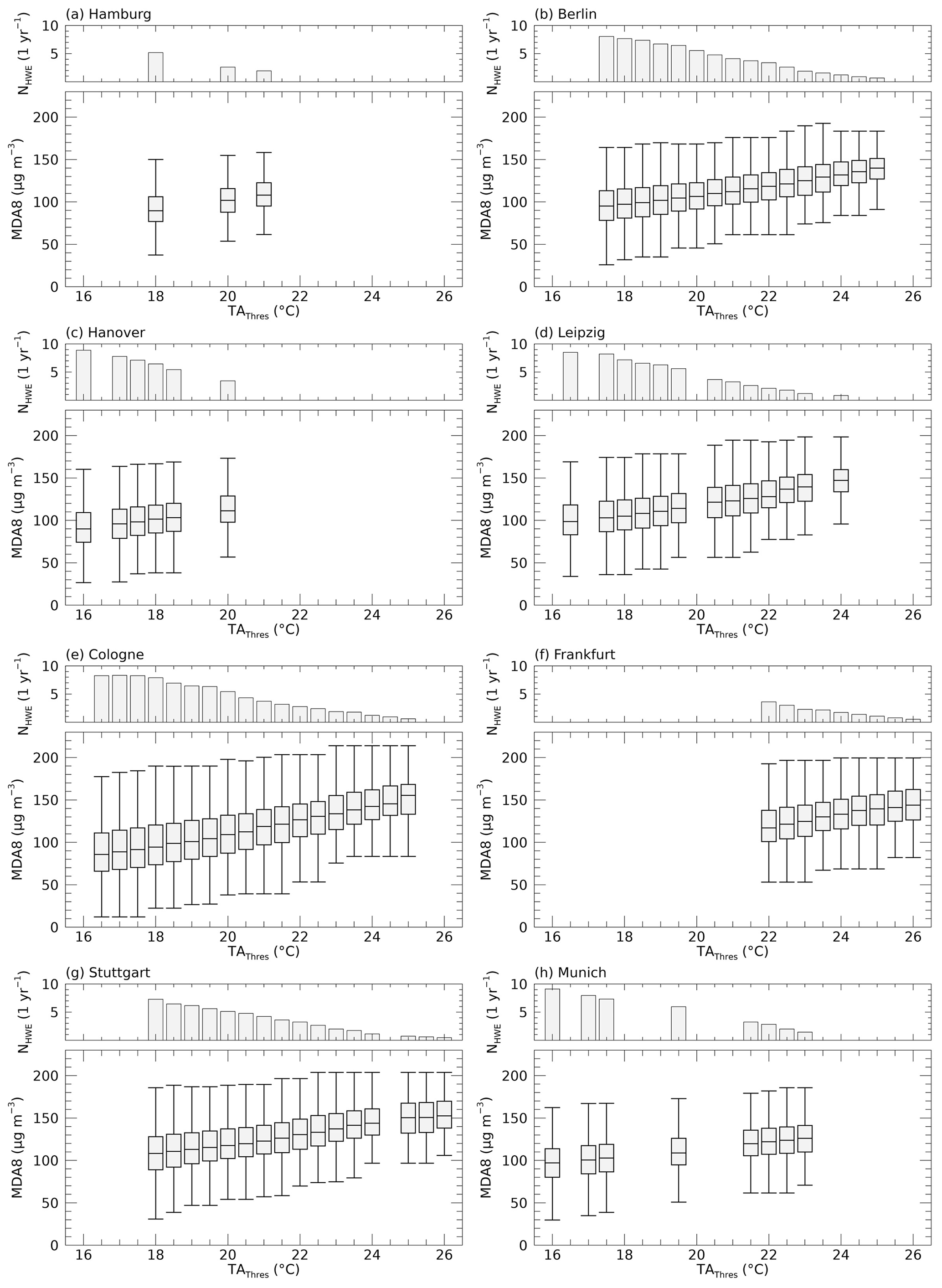
Figure 4 Top row of each panel: average number of HWEs per year (y axis), detected per TA_Thres (x axis). Box-and-whisker plots display daily values of MDA8 during detected HWEs. Boxes refer to the range between the 25th and 75th percentile (inter quartile range IQR), median values are given as solid lines, and whiskers are the minimum and maximum values excluding outliers (less than $Q\mathrm{1}-\mathrm{1.5}\cdot$ IQR, greater than $Q\mathrm{3}+\mathrm{1.5}\cdot$ IQR). Only results of overall statistically significant (F test, p< 0.05) MLR models are shown.

4.3 Inter-city differences

The strongest associations between TA_Mag as well as MDA8_M and mortality rates were found for Berlin, Cologne, Frankfurt and Stuttgart. These cities are also those in which the highest values of the 50th and 95th percentile and the maximum TA are recorded (Table 1). Based on absolute TA_Thres, it is not clear whether the lower effect observed in Hamburg, Hanover, Leipzig and Munich is reasoned by the absence of HWEs with TA_Thres > 24 ^∘C (Leipzig, Munich) or TA_Thres > 22 ^∘C (Hamburg, Hanover), which occur in other cities and show the strongest relationships to mortality rates.

Heterogeneities across cities were obtained not only for city-specific absolute TA_Thres but also for their respective values of r², which is also reported in other studies investigating other cities across Europe (e.g., Filleul et al., 2006; Baccini et al., 2011; Burkart et al., 2013; Breitner et al., 2014; Analitis et al., 2018; Scortichini et al., 2018). City-specific peculiarities such as demographic or socio-economic characteristics at the community level may cause these differences (Stafoggia et al., 2006; Anderson and Bell, 2011; Baccini et al., 2011). For instance, differences in age structure may influence the results. Elderly people were shown to be more vulnerable to heat (Yu et al., 2010; Scherer et al., 2013; Benmarhnia et al., 2015). Thus, a higher ratio of elderly people may strengthen the mortality rate during HWEs. The ratio of the elderly over 65 years is in fact heterogeneous among the involved cities (Table 1). Yet, a linkage to city-specific relation to the effect on mortality rates cannot be deduced. Heterogeneities across cities may also be caused by local-specific geographical characteristics. The close distance to the North Sea and Baltic Sea, associated with a maritime climate, may prevent Hamburg from air temperatures that lead to higher impacts on mortality rates as observed for other cities. Similarly, Munich is the city not only situated at the highest altitude in this study but also closest to the Alps, which may influence local weather conditions and lead to weather characteristics resulting in weaker relations between high air temperature and mortality rates. However, these reasons remain hypothetical and do not explain the low impacts in Hanover and Leipzig. To sum up, differences between cities are conceivable to be an overlap of city-specific characteristics, such as demographic and geographic factors.

Results of this study underline the complexity to find similarities across different cities to determine appropriate criteria to identify hazardous episodes in terms of a health-related adverse effect, if there was such an effort. Some cities show a strong relationship between TA_Mag and mortality rates, but these are also the cities experiencing the highest air temperatures in this study (Table 1). Moreover, the strength of this relationship also varies across cities for equal TA_Thres values. However, most similarities arise by comparing results based on their local-specific percentile of the air temperature distribution rather than using absolute thresholds. Further, this also includes the interactive contribution of ozone.

Further research is needed to investigate local characteristics in more detail such as geographic drivers, socio-economic or socio-demographic factors which may affect the air-temperature–ozone–mortality relationship. These may cause local heterogeneities. Further, some studies also identified other air pollutants that affect mortality during HWEs. Especially, concentrations of particulate matter were also found to be increased during episodes of hot and dry weather (Tai et al., 2010; Schnell and Prather, 2017; Kalisa et al., 2018). Enhanced emission of secondary fine particles during hot weather conditions accompanied with reduced air movement may lead to this increased concentration especially in urban areas. Further, particulate matter is also associated with adverse mortality effect and is thus additionally relevant to human health during HWEs (Burkart et al., 2013; Analitis et al., 2014; Schnell and Prather, 2017; Analitis et al., 2018).

5 Conclusions

This study investigated mortality rates during HWEs in eight cities in Germany from 2000 to 2017. HWEs were identified with a risk-based approach as a result of regressions between daily average air temperature above a threshold and mean mortality rates during these episodes. HWEs and thereby statistically significant regressions were detected in all selected cities for various air temperature thresholds. Results reveal a strong increase in the association around the 95th percentile of the local-specific air temperature distribution. Apart from air temperature, ozone concentrations were shown to contribute to mortality rates during HWEs. While air temperature was identified to be the dominant factor for elevated mortality rates, ozone concentrations alone contribute to those by up to 20 %. Additionally, results reveal that the effect of both stressors on mortality cannot be separated in many cases, highlighting their strong interaction. Especially for HWEs identified via higher threshold values of air temperature, ozone mostly contributes to mortality rates statistically inseparable from air temperature. To which extend air temperature and ozone explain mortality rates differs across cities and for various air temperature thresholds. Some cities show weak associations, while the contributions of both stressors to mortality rates are more pronounced in others. This study underlines the complexity to deduce one universal threshold value in order to identify potentially hazardous HWEs in terms of a health effect. Yet, it also emphasizes that besides air temperature ozone contributes to mortality during HWEs in German cities. Future research should focus on city-specific characteristics such as population characteristics or geographical peculiarities, which are likely leading to heterogeneities across cities and which may influence the respective air-temperature–ozone–mortality relationship.

Appendix A

Figure A1 Location of selected air temperature and ozone measurement sites in the investigated cities. Land cover classification is based on CORINE 2018, v20 (EEA, 2019b).

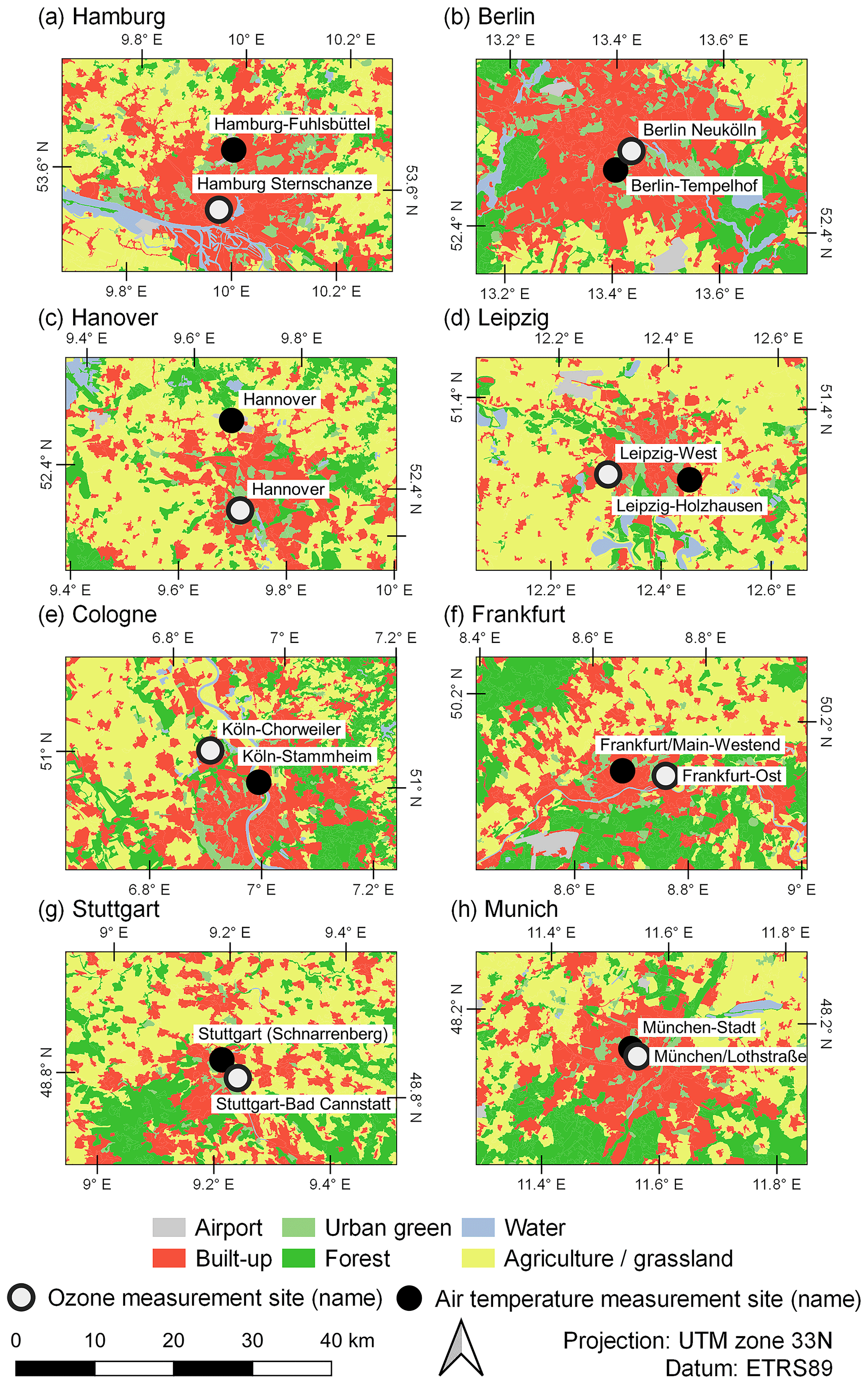
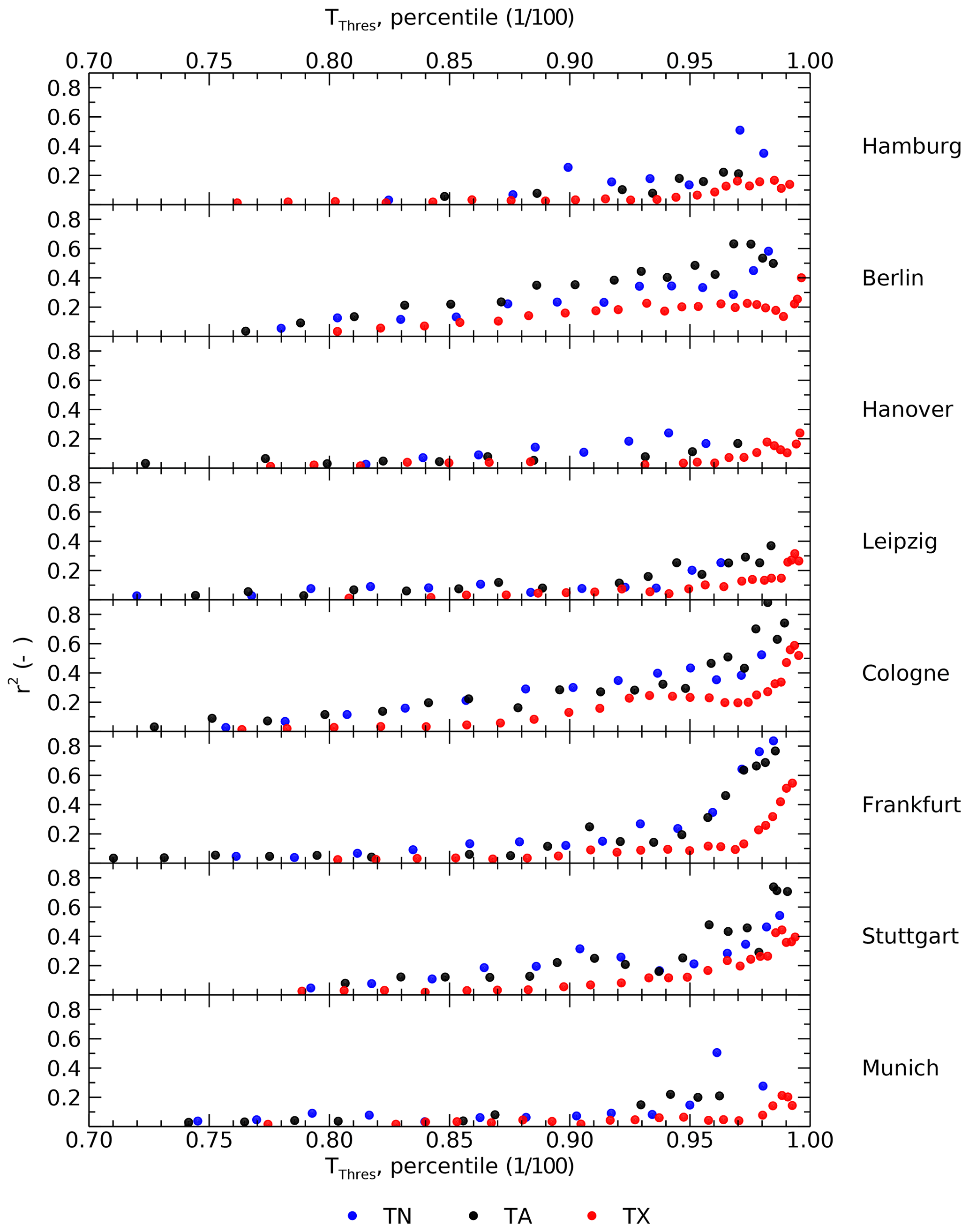
Figure A2 Comparison of regression analysis based on different predictor variables daily minimum air temperature (TN, blue), daily average air temperature (TA, black) and daily maximum air temperature (TX, red). Each panel displays results for one city. x axis: percentile of the respective air temperature distribution, y axis: explained variance (r²) of regression models.

Table A1 Selected air temperature and ozone measurement sites of each city. Air temperature data were obtained from the German Weather Service (DWD) (DWD, 2019); data of ozone concentrations were obtained by the German Environment Agency (UBA), based on originally measured data of air quality networks of the German federal states.