the Creative Commons Attribution 4.0 License.
the Creative Commons Attribution 4.0 License.
 | 12 Oct 2020
A novel approach to assessing nuisance risk from seismicity induced by UK shale gas development, with implications for future policy design
Maximilian J. Werner
We propose a novel framework for assessing the risk associated with seismicity induced by hydraulic fracturing, which has been a notable source of recent public concern. The framework combines statistical forecast models for injection-induced seismicity, ground motion prediction equations, and exposure models for affected areas, to quantitatively link the volume of fluid injected during operations with the potential for nuisance felt ground motions. Such (relatively small) motions are expected to be more aligned with the public tolerance threshold for induced seismicity than larger ground shaking that could cause structural damage. This proactive type of framework, which facilitates control of the injection volume ahead of time for risk mitigation, has significant advantages over reactive-type magnitude and ground-motion-based systems typically used for induced seismicity management. The framework is applied to the region surrounding the Preston New Road shale gas site in North West England. A notable finding is that the calculations are particularly sensitive to assumptions of the seismicity forecast model used, i.e. whether it limits the cumulative seismic moment released for a given volume or assumes seismicity is consistent with the Gutenberg–Richter distribution for tectonic events. Finally, we discuss how the framework can be used to inform relevant policy.
- Article
(4584 KB) - Full-text XML
- BibTeX
- EndNote


Awareness and concern regarding the impacts of seismicity induced by hydraulic fracturing have grown significantly in recent years (e.g Ellsworth, 2013; Davies et al., 2013; Cotton et al., 2014; Whitmarsh et al., 2015; Williams et al., 2017; Atkinson et al., 2020), which may pose a threat to the future development of unconventional gas resources (Kraft et al., 2009). There is evidence that tolerance of such operations will be increased if the public is made aware of the potential consequences of the resulting ground shaking (Giardini, 2009; Bommer et al., 2015). In addition, understanding these consequences is critical for responsible decision-making by relevant political authorities (e.g. MacRae, 2006). It is therefore essential to develop methodologies for quantifying and managing the hazard and risk posed by hydraulic-fracture-induced seismicity.
Several hazard and risk assessment procedures have already been proposed in the literature for various types of induced seismicity. For example, Douglas and Aochi (2014) developed a conceptual model for assessing the risk of generating felt or damaging ground motions from enhanced geothermal systems (EGSs), based on fluid injection rate. The model used information on recent seismicity and ground shaking predictions from a ground motion prediction equation (GMPE) to obtain a real-time hazard curve, which was combined with a fragility curve to quantify risk. Gupta and Baker (2019) developed a probabilistic framework for estimating regional risk due to induced seismicity related to wastewater injection in Oklahoma that extends conventional probabilistic seismic hazard analysis to account for spatiotemporally varying seismicity rates. Walters et al. (2015) developed a qualitative risk assessment framework for triggered seismicity related to saltwater disposal and hydraulic fracturing that included risk tolerance matrices to be considered by different stakeholders.
This paper proposes a novel risk assessment framework for hydraulic-fracture-induced seismicity that directly links the volume of fluid injected during an operation to its potential for causing nuisance ground motions, i.e. shaking that is an inconvenience to society and may raise annoyance or distress among the public (Foulger et al., 2018). This type of shaking is expected to be more in line with public tolerances for induced seismicity than larger ground motions that have the potential to cause structural damage (Bommer et al., 2015). The framework integrates, in a mathematically rigorous manner, statistical forecast models for injection-induced seismicity, ground motion prediction equations for hydraulic fracturing, and exposure models for nearby areas.
The framework is applied to the region surrounding the Preston New Road (PNR) shale gas site in Lancashire, North West England, where recent (2018/2019) hydraulic fracture operations resulted in 29 seismic events with local magnitude (ML) greater than 0 (e.g. Clarke et al., 2019), including eight that were felt by the local population (Baptie, 2019). We demonstrate how the risk calculations can accommodate numerous styles of potential decision-making related to the regulation of hydraulic-fracture-induced seismicity, and we investigate the sensitivity of the calculations to certain model assumptions. The paper ends with a discussion on ways in which the proposed framework could be used to design future policies related to the management of hydraulic-fracture-induced risk in the UK.
The proposed framework is a modified version of conventional probabilistic seismic hazard analysis (Cornell, 1968), where the rate of earthquake occurrence, the distribution of magnitudes, and therefore the rate of exceedance for a given intensity measure (IM) are conditioned on the total volume of fluid injected during a hydraulic fracture operation (Vt). It may be expressed as follows:
where ns is the number of earthquake sources, is the rate at which a exceeds b given the occurrence of c, Mi is the magnitude distribution for the ith source, p(k|j) is the probability of k given j, mmin is the minimum magnitude considered, is the maximum magnitude considered for a given injection volume, fY(y) is the probability density function of Y evaluated at y, and Ri is the distance distribution of distances from the ith source to the location of interest. The “” and “” terms are characterized by a statistical forecast model for injection-induced seismicity, the “” term is derived from ground shaking estimations by a GMPE designed for hydraulic fracturing events, and the “” term is obtained from an exposure model of the affected region. While the framework is sufficiently flexible to cater for any intensity measure, we specifically use peak ground velocity (PGV) as the measure of ground shaking in this study (i.e. IM is equal to PGV in Eq. 1) because of its close correlation with seismic intensity (Van Eck et al., 2006) and its ability to indicate damage for the small, shallow earthquakes of interest in this study (Bommer and Alarcon, 2006; Crowley et al., 2018).
The framework is based on the assumption of a one-to-one relationship between the exceedance of tolerable ground shaking thresholds and nuisance risk, i.e.
where NRi is the nuisance risk associated with the ith tolerable ground shaking threshold, xi. Tolerance for potential ground shaking may be dependent on the culture of those affected (Foulger et al., 2018), and a discussion with local stakeholders is therefore necessary to decide exactly what risk is acceptable (Giardini, 2009). However, our methodology provides a number of suggested tolerable ground shaking thresholds, based on previous studies associated with discomfort due to ground shaking (Bommer et al., 2006) and nuisance limits adopted for other types of vibration. These are (1) PGV=0.9 mm s−1, which approximately corresponds with the velocity at which pile driving becomes “barely perceptible” (Athanasopoulos and Pelekis, 2000); (2) PGV=3 mm s−1, which is the velocity at which traffic-induced vibration becomes “barely noticeable” (Barneich, 1985); (3) PGV=15 mm s−1, which is the lowest threshold of cosmetic damage for weak (i.e. unreinforced or light framed) structures, according to BSI (1993), and has been used in previous risk calculations for induced seismicity (Ader et al., 2020); and (4) PGV=50 mm s−1, which is the BSI (1993) threshold of cosmetic damage for strong (i.e. reinforced or framed) structures.
We apply the proposed framework to the region surrounding the Preston New Road (PNR) shale gas site in Lancashire, North West England, where hydraulic fracturing operations in late 2018 (at PNR-1z well) and mid-2019 (at PNR-2 well) resulted in 29 ML>0 events with maximum magnitude ML=2.9, eight of which were felt nearby (e.g. Baptie, 2019; Cremen et al., 2019a, b; Clarke et al., 2019; Kettlety et al., 2020). Shale gas development is a relatively new source of induced seismicity in the UK (Clarke et al., 2014), and the PNR activities are the only hydraulic fracturing operations to take place onshore in the country between a 2012 government-ordered investigation into the related risks (Mair et al., 2012) and the hydraulic fracturing moratorium imposed in England in November 2019. For the purposes of this application, we assume that seismicity is produced from a point source 2 km deep (i.e. ns=1 in Eq. 1), at a respective latitude and longitude of 53.7873∘ N and 2.9511∘ W. This location corresponds to the approximate depth of the Bowland shale targeted by the operation and the surface coordinates of the PNR-1z well, according to the 2018 hydraulic fracture plan of the operator (Cuadrilla, 2017).
3.1 Source and ground motion modelling
We use the Hallo et al. (2014) injection-volume-based statistical model of event magnitudes, as it was used for real-time seismicity forecasting by the operator during hydraulic fracturing at PNR (Clarke et al., 2019). This model assumes that the cumulative seismic moment released (∑Mo) is related to the total volume of fluid injected (Vt) as follows:
where μ is the rock shear modulus. SEFF depends on the medium type and the nature of the injected material and represents the ratio of ∑Mo to its theoretical maximum (μVt) if there was no aseismic deformation (Hallo et al., 2012). For this formulation,
where Mjo is the seismic moment equivalent of the jth earthquake and n is the number of earthquakes that occur, which is a random variable that follows a Poisson probability mass function with mean from Eq. (1). in Eq. (1) for the ith event is defined as
where αi−1 is the fraction of ∑Mo,w, the total seismic moment in moment magnitude terms, still to be released after the occurrence of the (i−1)th event.
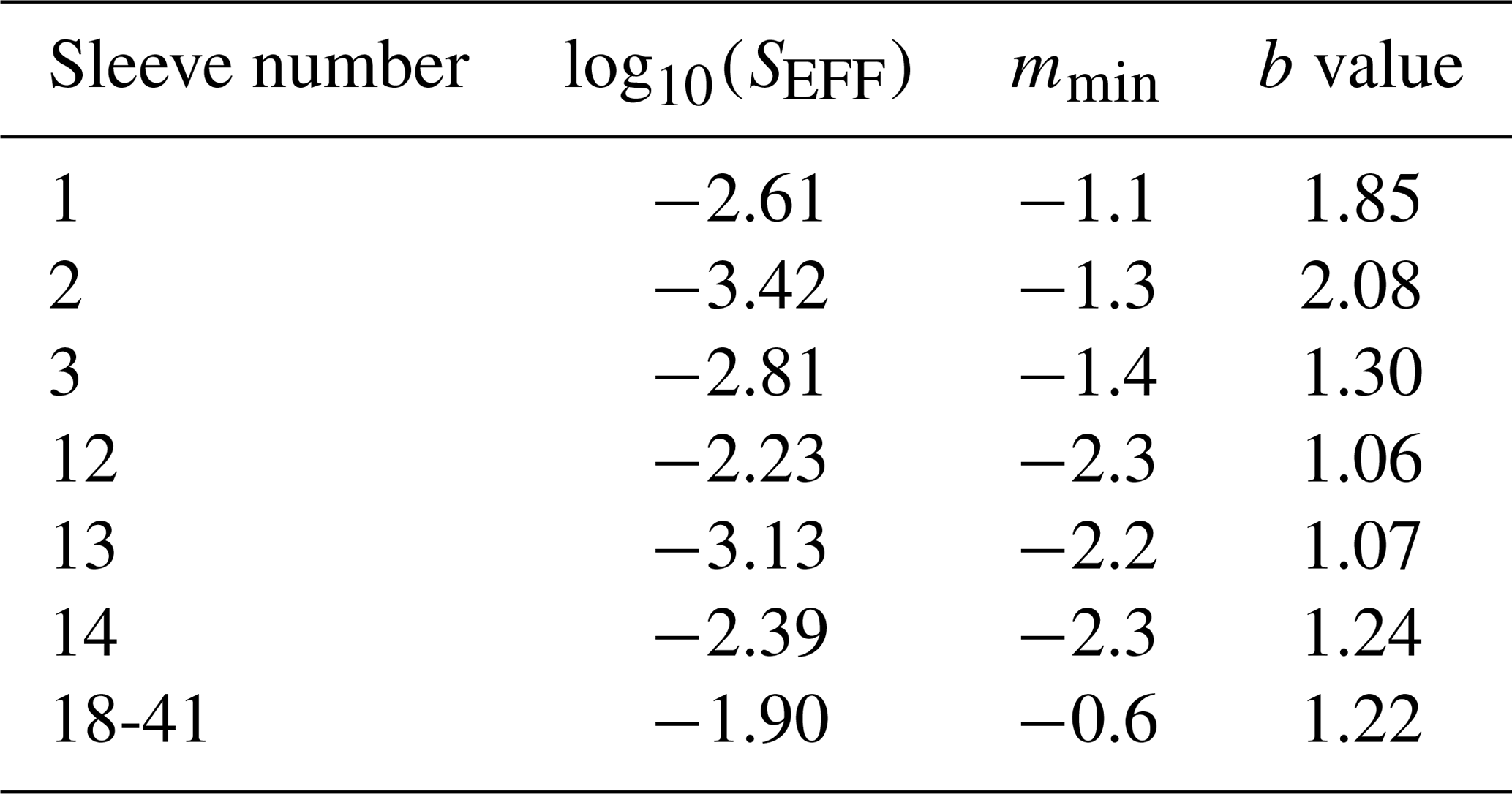
μ is assumed to be 20 GPa, from previous work on PNR seismicity (Clarke et al., 2019). The sets of SEFF, mmin, and b values used are those fit by Clarke et al. (2019) for seismicity produced during PNR-1z operations, where 17 sleeves were stimulated with a total injection volume of approximately 4200 m3 (see Table 1). We treat the stimulated sleeves before sleeve 18 (i.e. sleeves 1, 2, 3, 12, 13, and 14) as independent, and we use the relevant set of sleeve-specific seismicity parameters for each. For the 11 remaining stimulated sleeves, we use the set of seismicity parameters fit over their cumulative injected volume, as they were found to intersect the same fault (Clarke et al., 2019). It should be noted that some sets of seismicity parameters used were fit using a mixture of event magnitudes reported on moment and local scales (Clarke et al., 2019), yet the size of forecasted events is always measured on the moment magnitude scale. This discrepancy is deemed acceptable, however, given that the precise relationship between the scales is yet to be established (Mancini et al., 2019).
Table 1Seismicity parameters used in this study, from Clarke et al. (2019).
Ground shaking ( in Eq. 1) is predicted using the ground motion prediction equation of Cremen et al. (2019b), which was specifically designed for hydraulic-fracture-induced seismicity in the UK. This equation characterizes ground motion intensity in terms of moment magnitude and hypocentral distance at the location of interest. It is intended to model ground motion amplitudes for events with Mw<3 at hypocentral distances < 6 km.
3.2 Exposure database
The considered exposure database (fR(r) in Eq. 1) comprises buildings located within a 5 km hypocentral distance of the event location (Fig. 1). Building data are obtained from Ordnance Survey (OS) mapping, accessed through the Edina Digimap service (Morris et al., 2000). Building footprint information is acquired from the “Buildings” layer of the OS VectorMap Local product, and building height information is acquired from the OS MasterMap “Building Height Attribute” database. Height and footprint data are matched via their geographic coordinates; we consider the corresponding building height for a given building footprint to be the closest located within 10 m. To exclude small uninhabitable structures, we neglect buildings with footprint areas < 40 m2 and/or known building heights < 3.5 m. This results in a final exposure database of 4195 buildings.
We also separately consider important buildings, or critical sites in which the occupants (or equipment) may be more sensitive to the effects of vibrations from ground shaking than those of conventional residential or commercial buildings (Walters et al., 2015; Ader et al., 2020). We exclusively focus on educational and medical facilities within 5 km of the event, which are identified from the “Important Buildings” layer of the OS VectorMap Local. We neglect all important buildings with footprint areas < 100 m2, which is the typical size of a classroom (Haylock, 2001). This results in a final database of six important buildings.
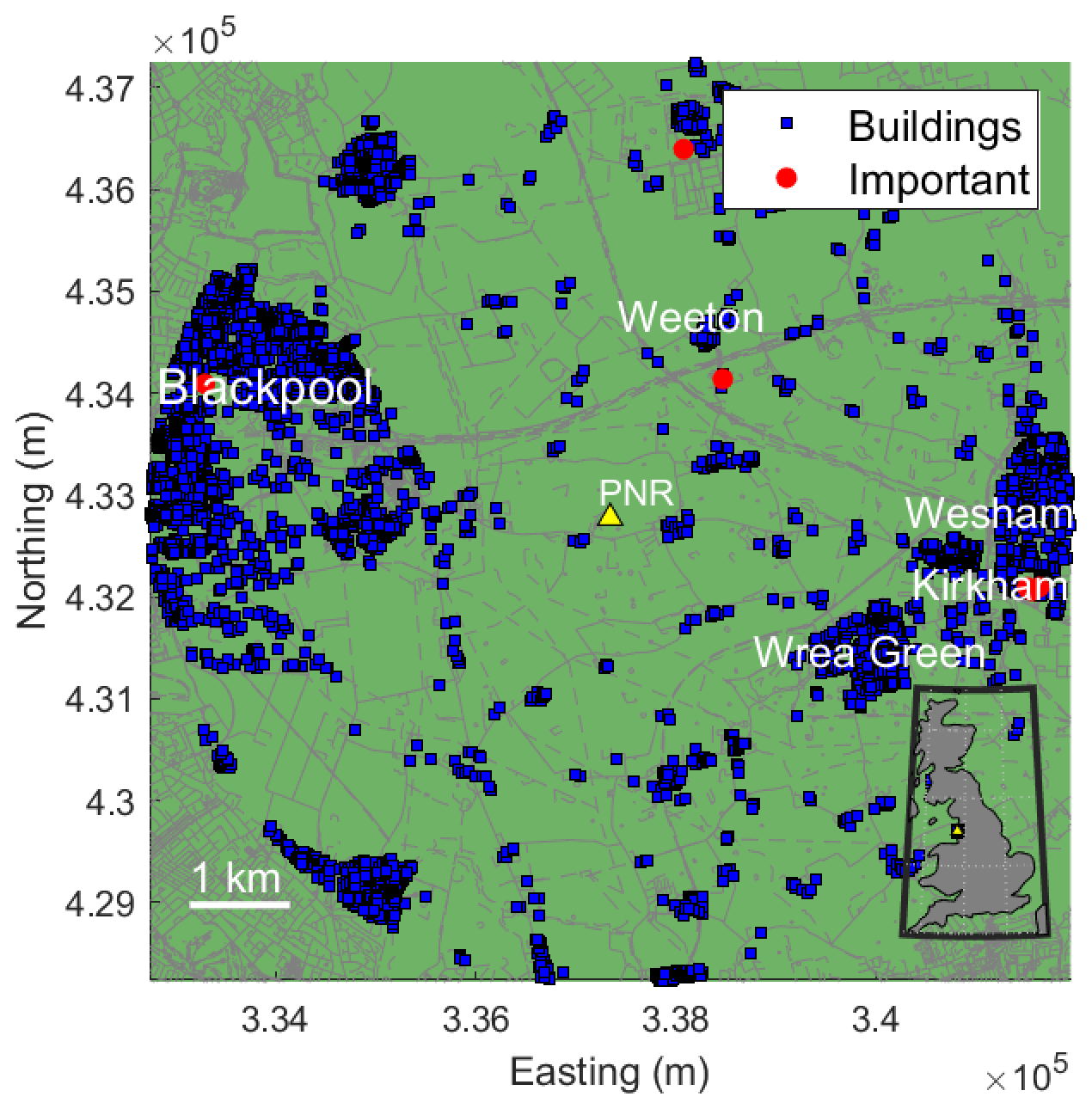
Figure 1All buildings and important (i.e. educational and medical) buildings considered within 5 km hypocentral distance of the case study event location at the Preston New Road (PNR) hydraulic fracture site (inset highlights location relative to all of Great Britain). ©OpenStreetMap contributors 2019 (https://www.openstreetmap.org/copyright, last access: September 2020).
3.3 Monte Carlo sampling procedure
Equation (1) describes ground motion exceedance at a single site. To capture the risk across the multiple buildings of interest in this study and correctly account for ground motion variability (Bourne et al., 2015), we employ a Monte Carlo sampling approach (e.g. Musson, 1999; Assatourians and Atkinson, 2013). This procedure involves the following steps for a given injection volume:
-
calculate the corresponding total seismic moment, using Eq. (3);
-
choose a single random event from the magnitude distribution of Eq. (1), which is truncated on the left by mmin and on the right by (as defined in Eq. 5);
-
use the Cremen et al. (2019b) GMPE to simulate a random inter-event variability and random intra-event variabilities for each site;
-
calculate median ground motion predictions from the GMPE at each site for the given combination of {m,r}, and add the inter- and intra-event variabilities generated in step 3 to simulate ground motion intensities;
-
repeat steps 2–4 until the total seismic moment of the sampled events is equal to that calculated in step 1 to within a small tolerance;
-
repeat steps 2–5 1000 times to generate 1000 potential catalogues corresponding to the given injected volume.
3.4 Modelling validation
The proposed risk modelling approach is validated using data observed during the 2018 hydraulic fracturing operations at the PNR-1z well. We complete the Monte Carlo sampling procedure for the actual volumes of fluid injected during those operations, using the UK Oil and Gas Authority's database on PNR operations (https://www.ogauthority.co.uk/onshore/onshore-reports-and-data/preston-new-road-pnr-1z-hydraulic-fracturing-operations-data/, last access: September 2020). Figure 2a–c compare the predicted numbers of earthquakes with those observed across selected sleeves (similar results are obtained for the remaining sleeves). It is seen that the observations almost always lie within the first and 99th percentile predictions of the model; thus we can conclude that the source model used is appropriate for forecasting the seismicity of interest.
Figure 2d compares ground shaking predictions at locations in the exposure model with observed ground motion amplitudes, for all forecasted/recorded events of , within a 2–3 km hypocentral distance range. This distance range is chosen since it corresponds to (1) a similar number of predictions (229 per synthetic catalogue) and observations (173) and (2) an almost identical mean hypocentral distance for predictions (2.66 km per synthetic catalogue) and observations (2.69 km). It is seen that the observed ground shaking amplitudes generally lie within the first and 99th percentile predictions, and therefore it is clear that the proposed model is adequately capturing the shaking intensity (risk) of interest. This confirms that the slight magnitude scale discrepancy in the source model (see Sect. 3.1) does not inhibit the overall performance of the calculations.
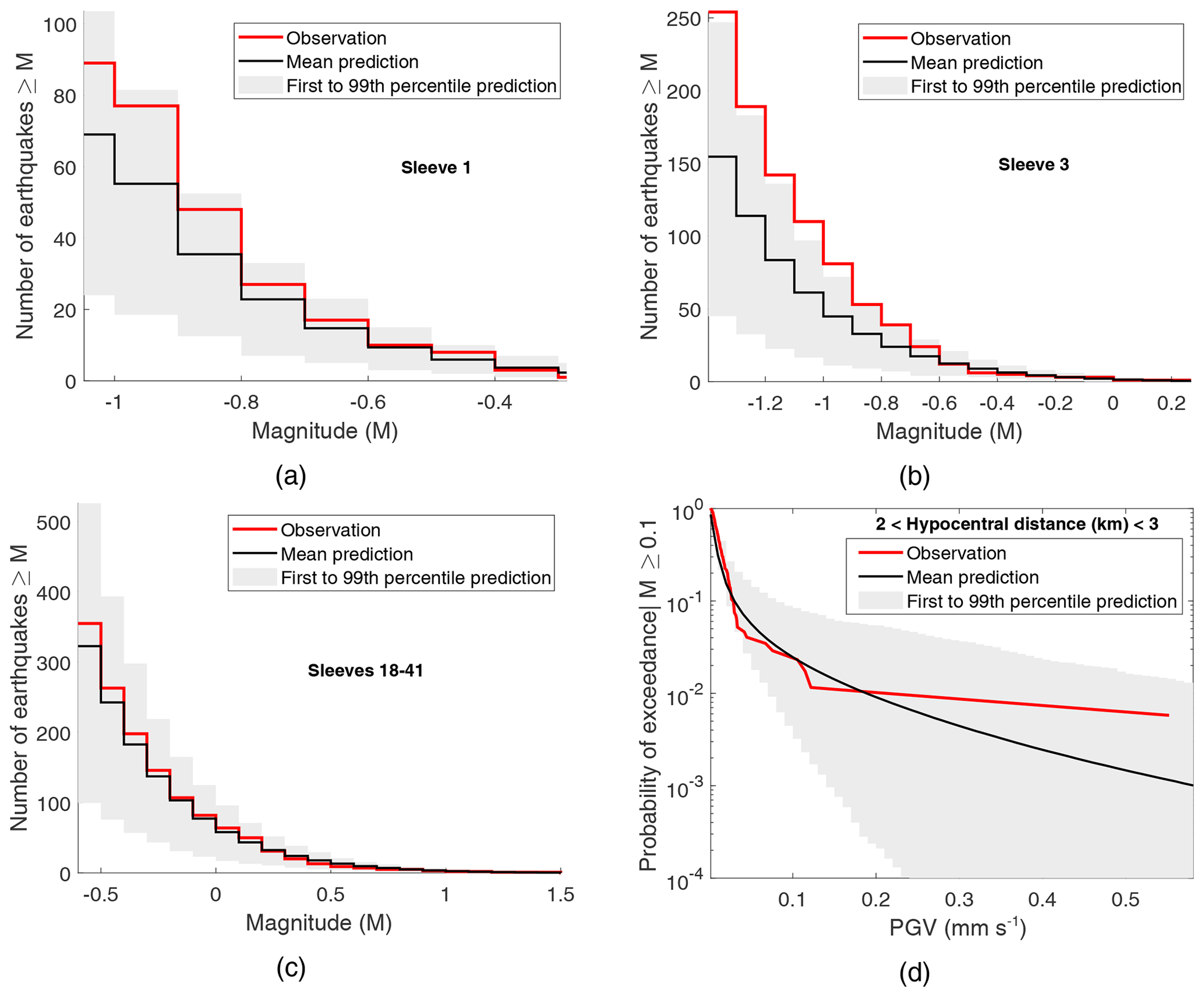
Figure 2Validating the risk modelling approach of this study, using data observed during hydraulic fracturing of the PNR-1z well. (a–c) Comparing forecasted numbers of earthquakes with those observed and (d) comparing predicted ground shaking with observed ground motion amplitudes.
4.1 Magnitude-specific calculations
We first examine the risk associated with the occurrence of specific moment magnitudes (Mw) up to Mw=3, which is the maximum applicable magnitude for the Cremen et al. (2019b) GMPE. We repeat steps 3 and 4 of Sect. 3.3 1000 times for Mw between 0.1 and 3, in increments of 0.1. Results of the calculations are found in Fig. 3, where they are presented three different ways to accommodate various potential styles of decision-making. Figure 3a–d summarize the probability of exceeding the prescribed risk thresholds at least once across different magnitude–distance bins, considering all buildings. As expected, the probability of exceeding the thresholds increases for increasing magnitude and decreasing hypocentral distance. It is observed that the PGV=0.9 mm s−1 (pile-driving perceptibility) threshold exceedance probability becomes non-negligible () for at close distances, and for at all examined distances. The PGV=3 mm s−1 (traffic noticeable) threshold exceedance probability becomes non-negligible () for and non-negligible at all examined distances for . The PGV=15 mm s−1 (cosmetic damage for weak structures) threshold exceedance probability becomes non-negligible () for and for at all distances of interest. The PGV=50 mm s−1 (cosmetic damage for strong structures) threshold exceedance probability becomes non-negligible () for but does not become non-negligible across all examined distances for any magnitude of interest in this study. Figure 3e and f examine the risk associated with three specific magnitudes: (1) ML=0.5, which is the current red light (“stop injection”) threshold for hydraulic-fracture-induced seismicity in the UK; (2) ML=2.1, which was the second-largest event that occurred during 2018/2019 PNR operations; and (3) ML=2.9, which was the largest event that occurred during 2018/2019 PNR operations. These magnitudes are converted to moment magnitude for input to the Cremen et al. (2019b) GMPE, using the empirical relationship derived by Butcher et al. (2019) for small magnitudes in a similar geologic setting; this is an approximate conversion, since the relationship between the scales is uncertain (Mancini et al., 2019). For this relationship, (1) ML=0.5 is equivalent to Mw=1.1, (2) ML=2.1 is equivalent to Mw=2.2, and (3) ML=2.9 is equivalent to Mw=2.7.

Figure 3Magnitude-specific risk calculations. Panels (a–d) summarize the probability of PGV exceeding the prescribed risk thresholds (0.9, 3, 15, and 50 mm s−1, respectively) at least once across different magnitude–distance bins; (e) highlights, for three specific magnitudes (i.e. Mw=1.1, Mw=2.2, and Mw=2.7), the probability of exceeding various PGV levels for at least one building (blue curves) and one important building (red curves); and (f) shows, for three specific magnitudes (i.e. Mw=1.1, Mw=2.2, and Mw=2.7), the average number of buildings (blue curves) and important buildings (red curves) at which various PGV levels are exceeded.
Figure 3e shows the probability of exceeding different PGV levels at least once, across all considered buildings (blue curves) and important buildings (red curves). It is seen that the current “red light” event for UK hydraulic fracturing has only a negligible (≈ 0.2 %) probability of exceeding the lowest of the four considered tolerable risk thresholds at the location of at least one building in the exposure model. An event equivalent in size to the second largest 2019 event will almost certainly exceed both the pile-driving and traffic thresholds and has a 2 % chance of causing cosmetic damage in a worst-case scenario (i.e. weak structure). An event equivalent in size to the largest 2019 event exceeds the first three considered tolerable risk thresholds with certainty, and there is an approximate 10 % chance that it will result in ground motions that cause cosmetic damage of at least one building in a best-case scenario (i.e. strong structure). The predicted occurrence of cosmetic damage for Mw=2.7 is consistent with actual observations (despite the hypothetical event being located approximately 0.8 km to the east of where the actual event occurred, at a 0.5 km shallower depth); the British Geological Survey assigned the event an intensity of 6 on the European Macroseismic Intensity scale (Grünthal, 1998), meaning “slightly damaging”, based on data from more than 2000 felt reports (British Geological Survey, 2019a).
It is also seen in Fig. 3e that the curves associated with important buildings are positioned to the left of those associated with all buildings, for the same magnitude event. This implies that the risk for important buildings is lower than that for all buildings. For example in the worst-case scenario, there is only approximately 10 % probability of cosmetic damage occurring in at least one important building vs. near certainty of this type of damage occurring in at least one building, for an event equivalent to the largest that occurred in 2019. The smaller risk associated with important buildings makes sense, since they are located further away from the hydraulic fracture site than the closest of all considered buildings (see Fig. 1).
Figure 3f shows the average number of all buildings (blue curves) and important buildings (red curves) at which different PGV levels are exceeded for the three specific magnitudes examined. Less than one building is expected to experience shaking that exceeds the lowest of the four considered tolerable risk thresholds, for an event equal in size to the current UK red light event. Approximately 30 buildings are expected to experience ground motions that exceed the traffic threshold for an event equivalent in size to the second largest that occurred in 2019, and approximately 20 buildings are expected to experience cosmetic damage in a worst-case scenario for an event equivalent in size to the largest in 2019. In the case of important buildings, fewer than one is expected to experience exceedance of the pile-driving threshold for either Mw=1.1 or Mw=2.2, and approximately one is expected to experience exceedance of the traffic threshold for Mw=2.7.
4.2 Injection-volume-based calculations
We use the procedure outlined in Sect. 3.3 to examine the risk associated with the following injection volumes: 500, 1000, 5000, 10 000, 15 000, 20 000, 30 000, 40 000, and 50 000 m3. These values capture the typical range of injection volumes planned/used for hydraulic fracturing operations in both the UK (Westaway, 2016; Cuadrilla, 2017, 2019; Third Energy, 2017; Clarke et al., 2019) and North America (Ground Water Protection Council, 2009; Johnson and Johnson, 2012; Precht and Dempster, 2012; Gallegos et al., 2015). We assume that each volume is divided evenly among the 17 stimulated sleeves of the PNR-1z operation, and we simulate seismicity according to the sleeve-dependent parameters discussed in Sect. 3. Results of the calculations are summarized in Fig. 4, using similar presentation methods as those introduced in Sect. 4.1.
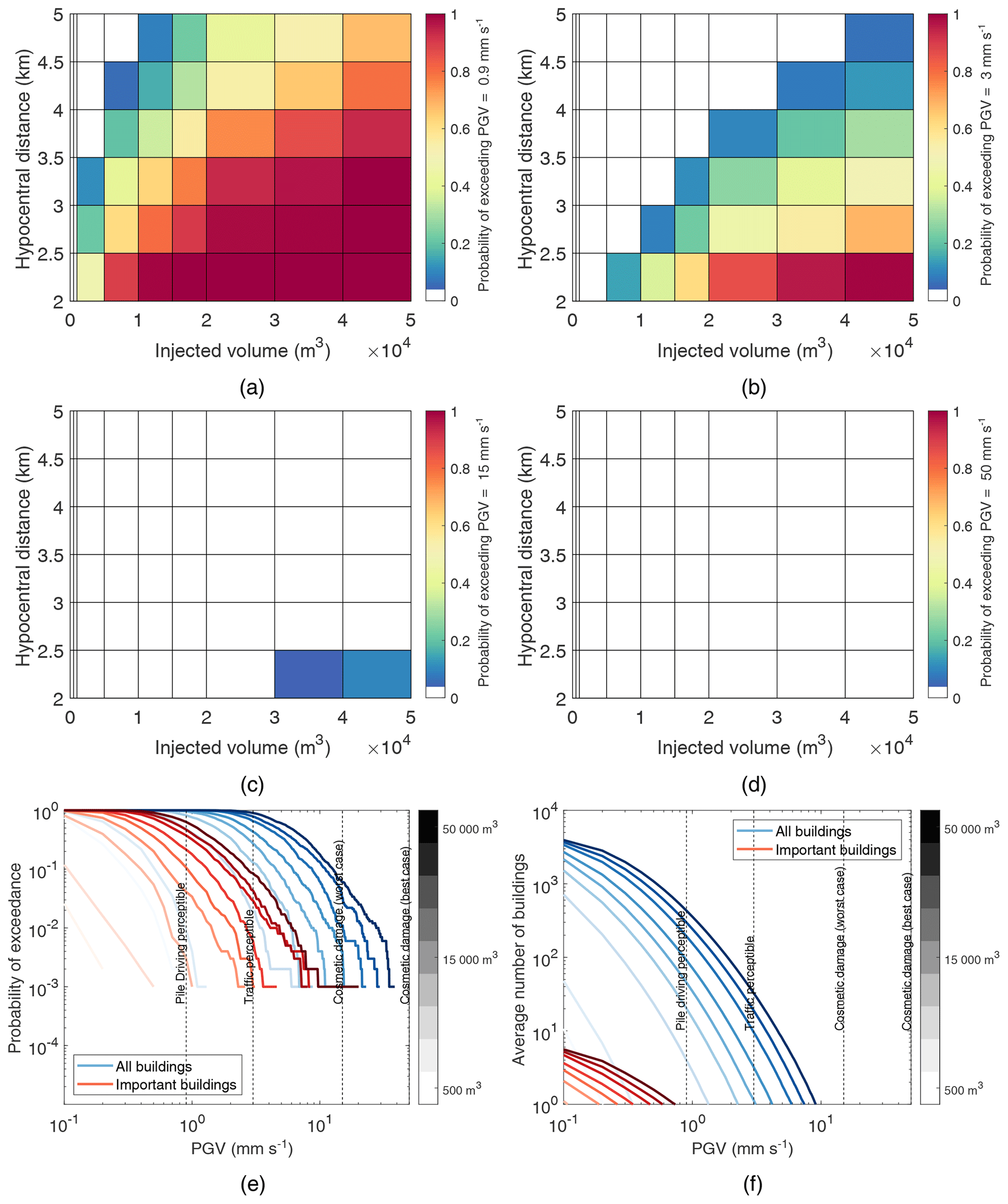
Figure 4Injection-volume-based risk calculations. Panels (a–d) summarize the probability of PGV exceeding the prescribed risk thresholds (0.9, 3, 15, and 50 mm s−1, respectively) across different volume–distance bins; (e) highlights, for specific volumes (i.e. 500, 1000, 5000, 10 000, 15 000, 20 000, 30 000, 40 000, and 50 000 m3), the probability of exceeding various PGV levels for at least one building (blue curves) and one important building (red curves); and (f) shows, for specific volumes (i.e. 500, 1000, 5000, 10 000, 15 000, 20 000, 30 000, 40 000, and 50 000 m3), the average number of buildings (blue curves) and important buildings (red curves) at which various PGV levels are exceeded.
Figure 4a–d show the probability of exceeding the prescribed risk thresholds at least once across different volume–distance bins, considering all buildings. The probability of exceeding the thresholds clearly increases as injection volume increases and hypocentral distance decreases, in line with expectations. The PGV=0.9 mm s−1 (pile-driving) threshold exceedance probability becomes non-negligible () at close distances for 1000 m3 of injected volume and at all examined distances for 10 000 m3. The PGV=3 mm s−1 (traffic) threshold exceedance probability becomes non-negligible () for 5000 m3 and non-negligible at all examined distances for 40 000 m3. The PGV=15 mm s−1 (cosmetic damage for weak structures) threshold exceedance probability becomes non-negligible () for 40 000 m3 but does not become non-zero across all examined distances for any injection volume of interest. The PGV=50 mm s−1 (cosmetic damage for strong structures) threshold is not exceeded for the examined injection volumes.
Figure 4e and f examine the risk associated with the specific injection volumes of interest, across different PGV levels. Figure 4e shows the probability of exceeding a given value of PGV at least once, across all considered buildings (blue curves) and important buildings (red curves). It is seen that there is no chance of exceeding any of the considered tolerable risk thresholds for 500 m3 injected volume, and there is approximately a 1 % probability of exceeding the lowest of the four considered thresholds at least once for 1000 m3. 5000, 10 000, 15 000, 20 000, and 30 000 m3 have approximately a 2 %, 10 %, 30 %, 50 %, and 80 % chance, respectively, of generating ground motions that exceed the traffic threshold at the location of at least one building in the exposure model. The largest two injection volumes considered (i.e. 40 000 and 50 000 m3) will almost certainly result in shaking that exceeds the traffic threshold, but will only result in cosmetic damage in a worst-case scenario (weak structure) with less than 10 % probability. It appears that no injected volumes examined have any chance of causing cosmetic damage in a best-case scenario (strong structure) (preliminary calculations suggest that approximately 80 000 m3 is required for a non-zero probability of this damage occurring). Curves associated with important buildings are positioned to the left of those associated with all buildings in Fig. 4e, implying lower risk for important buildings as discussed in Sect. 4.1. For example in the worst-case scenario, there is negligible (≈0.1 %) chance of cosmetic damage occurring in at least one important building vs. approximately 9 % probability of this type of damage occurring in at least one building, for the largest considered injected volume.
Figure 4f shows the average number of all buildings (blue curves) and important buildings (red curves) at which different PGV levels are exceeded for the injection volumes examined. Fewer than one important building is expected to experience shaking that exceeds the lowest of the four considered tolerable risk thresholds for any injected volume analysed, and fewer than one building of any type is expected to experience exceedance of this threshold for both 500 and 1000 m3 injected volumes. Fewer than 10 buildings are expected to experience exceedance of the lowest threshold for 5000 m3, and between 10 and 100 buildings are expected to experience shaking above this threshold for 10 000, 15 000, and 20 000 m3. Between 10 and 100 buildings are expected to experience exceedance of the traffic threshold for the 30 000, 40 000, and 50 000 m3. Fewer than one building is expected to experience cosmetic damage in a worst-case scenario, for any injected volume examined.
We disaggregate the results shown in Fig. 4 and examine the risk associated with each injection volume in terms of the frequency of risk threshold exceedances attributable to different event magnitudes (Bazzurro and Allin Cornell, 1999). Frequencies of exceedance are important to consider, given that the number of shaking episodes people experience is expected to directly influence their tolerance limit (Bommer et al., 2006); a single occurrence of ground shaking with relatively high intensity may be significantly less concerning to local populations than a continuous series of weaker felt ground motions (Bourne et al., 2015).
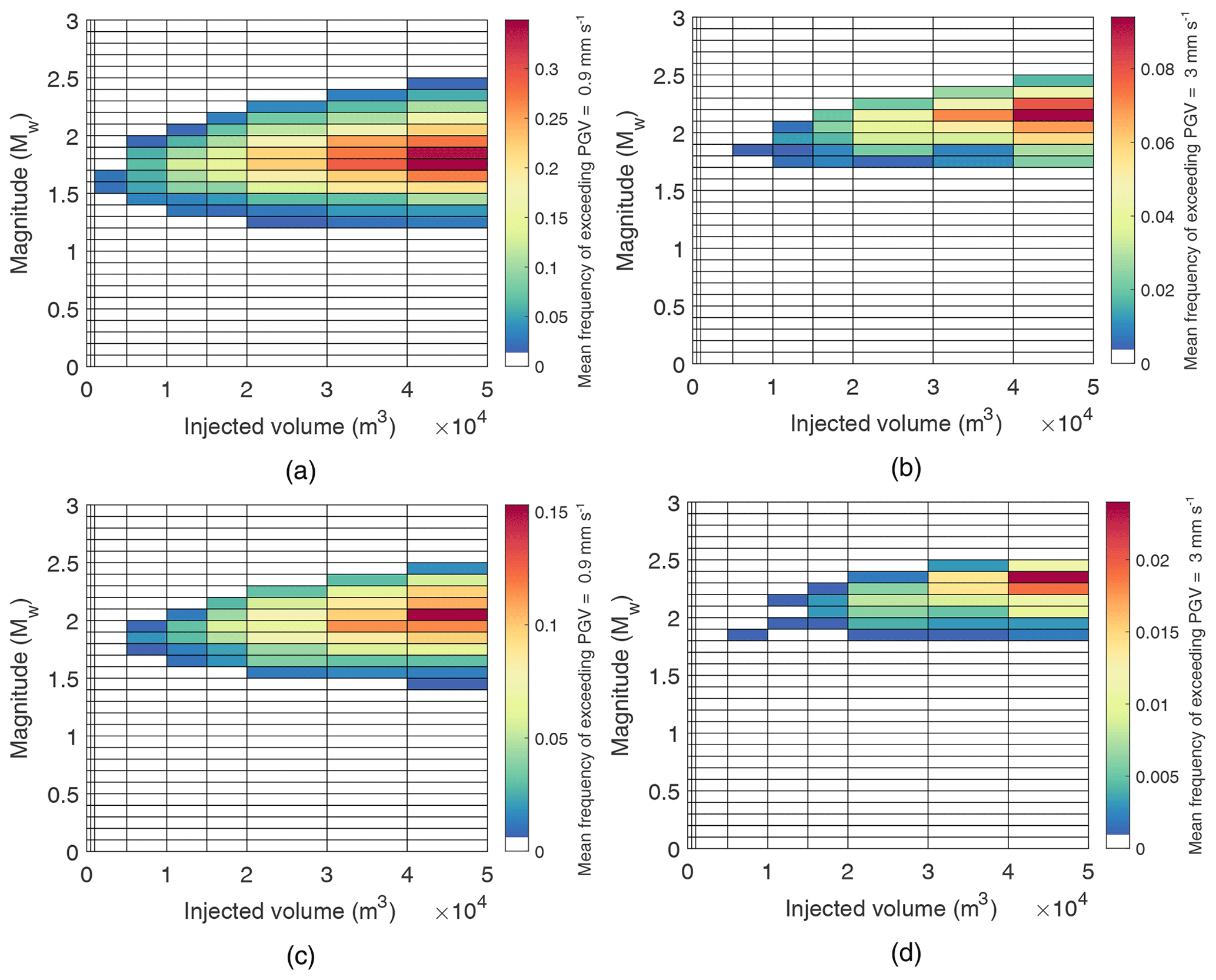
Figure 5Ground motion disaggregation for PGV=0.9 mm s−1 (a, c) and PGV=3 mm s−1(b, d) risk thresholds, across (a, b) all buildings and (c, d) important buildings.
We provide the results of the disaggregation in Fig. 5 for the PGV=0.9 mm s−1 and the PGV=3 mm s−1 thresholds. These plots show, for each injected volume of interest across different magnitudes, the average number of events per catalogue associated with ground shaking that exceeds the risk threshold of interest at the closest building (or important building) in the exposure model to the location of seismicity. It is clear that the largest contributor to exceeding either threshold is not always the maximum magnitude experienced, particularly for larger volumes of injected fluid. For example, for all considered buildings and an injected volume of 50 000 m3, Mw2.2 events result in approximately 4 times the number of traffic threshold exceedances than Mw2.5 earthquakes. Intermediate magnitudes govern the hazard and risk because they occur more frequently than larger magnitudes. In line with previous studies (Bourne et al., 2015), the findings of the disaggregation underline the fact that it is not always useful to focus exclusively on the maximum magnitude parameter (e.g. McGarr, 2014) when assessing the risk due to induced seismicity.
The application of the proposed risk framework presented in Sects. 3 and 4 made use of a number of assumptions related to the source modelling and prediction of ground motion. For example, we assumed that all seismicity was co-located and that there were no spatial correlations in the ground motions from a given event. Alternative assumptions may also be valid however, depending on the level of information available at the time a risk analysis is being conducted. This section explores the impact of some of these assumptions on the risk calculations. We first discuss the alternative assumptions of interest, and we present the results of their impact for all considered buildings in the exposure model across 5000, 20 000, and 50 000 m3 of injected fluid in Fig. 9. In all cases, injection volume is divided evenly between sleeves as in Sect. 4.2.
5.1 Uncertain seismicity parameters
The analysis conducted in Sect. 4.2 relied on after-the-fact observation-based estimates of b and SEFF and the value of μ used in a previous study of the same seismicity. In reality however, there is likely to be a large degree of uncertainty in these parameters before operations are carried out (e.g. Bommer et al., 2015; Mignan et al., 2017), when we expect the proposed risk assessment procedure to be at its most valuable in forecasting nuisance risk associated with planned injection volumes. It is therefore important to understand how uncertainties in these parameters affect the calculations of the framework. To do this, we conduct a hypothetical a priori risk assessment, in which rational uncertainties in the seismicity parameters are introduced.
We assume a uniform distribution of b values between 1 and 2. This is a sensible approach, given that the bounds of the distribution approximately represent the two opposite conditions of fault reactivation within a seismically active region (i.e. b=1) and hydraulic fracture interaction with natural fractures (i.e. b=2) (Eaton et al., 2014; Chen et al., 2018). We assume a uniform distribution of log 10(SEFF) values between −4 and −1. The chosen bounds are within the limits of those expected for hydraulic fracturing and enhanced geothermal systems (Hallo et al., 2014), which the values for hydraulic fracturing may reach in extreme cases (Hallo et al., 2012). They are also in line with the range of values observed during the hydraulic fracturing operation studied in Verdon and Budge (2018). Finally, we assume a uniform distribution for μ between 10 and 20 GPa, in accordance with the sample of shear moduli values obtained in a geomechanical study of Bowland shale (De Pater and Baisch, 2011).
Uncertainty in the seismicity parameters affects steps 1, 2, and 6 of the Monte Carlo sampling procedure (Sect. 3.3). In step 1, single random SEFF, b, and μ values are chosen from their respective distributions. The chosen SEFF and μ values are used to calculate the total seismic moment for the given injection volume, and the sampled b value is used to characterize the distribution used in step 2. In step 6, steps 1–5 are instead repeated, such that each synthetic catalogue is generated from different seismicity parameter values.
5.2 Uncertain event locations
We have thus far assumed that the location of seismicity is known and that all events are co-located in space. In realistic scenarios however, there will be some uncertainty on event locations (e.g. Bao and Eaton, 2016; Verdon et al., 2019). To explore the impact of this uncertainty on the risk calculations, we repeat the analyses for random event locations.
We assume events are produced from point sources that are uniformly distributed within 1.4 km of the surface coordinates of the PNR-1z well, where 1.4 km corresponds to the lateral length of the PNR-1z well (1 km) (Cuadrilla, 2017) plus the distance of the largest event from the injection point (400 m) during previous hydraulic fracturing at a nearby shale gas site (Clarke et al., 2014). (The maximum distance between the surface coordinates of the PNR-1z well and the 57 events detected by the British Geological Survey (BGS) surface array during 2018 hydraulic fracture operations was 1.38 km, which further confirms that 1.4 km is a sensible distance cap to assume.) A uniform distribution is chosen to accommodate hypothetical cases in which the direction of the intended well path is still unknown.
Event depths are assumed to be uniformly distributed between 1.5 and 3 km. This is a reasonable approach, given that the bounds of the distribution approximately correspond to the maximum and minimum depths of shale at the PNR site (Cuadrilla, 2017). Note that the Cremen et al. (2019b) GMPE is not strictly intended for hypocentral distances < 2 km; however we deem its use in such cases acceptable here in the absence of an appropriate alternative model that has been calibrated for such shallow depths and given that these distances comprise less than 0.3 % of all those simulated within 5 km.
Accounting for event location uncertainty requires an additional task in the Sect. 3.3 Monte Carlo risk procedure between steps 1 and 2, in which single distance-to-well and depth values are sampled from their respective assumed distributions to generate a random earthquake location. The exposure database examined also varies for each event; assessed buildings are selected according to the same hypocentral distance, height, and footprint criteria discussed in Sect. 3.2.
5.3 Different rupture behaviour
The statistical earthquake forecast model used in our analysis assumed a deterministic limit on earthquake magnitudes, based on the volume of fluid injected (see Eq. 5). While this model performed well for forecasting events during 2018 operations at PNR (see Sect. 3.4; Clarke et al., 2019) and closely aligned with observations when applied in a pseudo-prospective manner for hydraulic fracture operations at Horn River in Canada (Verdon and Budge, 2018), there is ample evidence in the literature to suggest that earthquakes may not be limited in size by the associated industrial activity (e.g. Gischig, 2015; Atkinson et al., 2016; Mignan et al., 2019; Lee et al., 2019).
We now test the implications on the risk calculations of instead using the van der Elst et al. (2016) source model for simulating events during fluid injection, which assumes that the largest magnitudes that occur for a given injection volume are consistent with the sampling statistics of the Gutenberg–Richter distribution for tectonic events. This approach was found to correspond well with magnitude–volume observations for recent fluid-induced seismicity during a geothermal stimulation in Finland (Kwiatek et al., 2019).
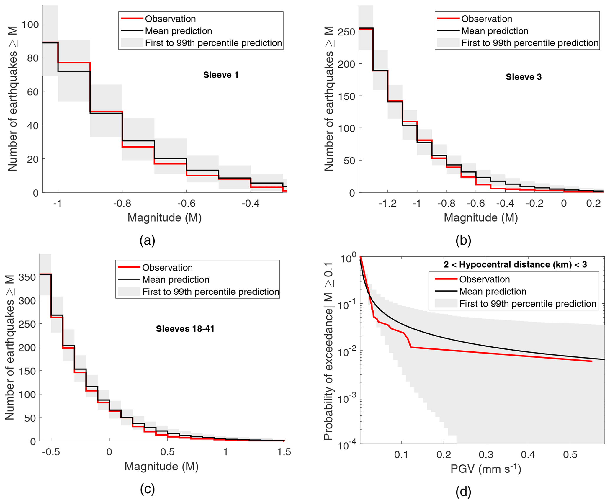
Figure 6Validating the van der Elst et al. (2016) approach as an alternative assumption about rupture behaviour for the case study. (a–c) Comparing forecasted numbers of earthquakes with those observed and (d) comparing predicted ground shaking with observed ground motion amplitudes.
The van der Elst et al. (2016) model is based on the Shapiro et al. (2010) seismogenic index (Si) equation, which is expressed as follows:
where N is the expected number of earthquakes larger than magnitude m that occur due to injected fluid volume Vt, and the Si parameter depends on the seismotectonic features of the region of interest. For this modelling approach, the “” term of Eq. (1) becomes
In the following calculations, we use the Si parameters that correspond to the sets of SEFF, mmin, and b values detailed in Sect. 3.1. All other parameters used are as defined previously. We first test the validity of the model (Fig. 6), using observed seismicity data for 2018 PNR fracture operations as outlined in Sect. 3.4. The observed data generally lie within the first and 99th percentile bounds of model predictions for both seismicity (similar results are found for sleeves not shown) and ground shaking. We thus conclude that the van der Elst et al. (2016) model is a reasonable alternative assumption about rupture behaviour for this case.
This assumption affects all steps of the Monte Carlo procedure in Sect. 3.3. In step 1 (which is now also repeated in step 6), the total number of earthquakes above mmin is simulated from a Poisson probability mass function with mean N (Eq. 6), which is the number of times steps 2–4 are repeated in step 5. In step 2, , which is the most likely maximum magnitude of UK tectonic earthquakes (Woessner et al., 2015). Steps 3 and 4 remain the same as in Sect. 3.3 if the sampled magnitude is less than 3, which is the maximum applicable magnitude for the Cremen et al. (2019b) GMPE. The Douglas et al. (2013) model 1 is used for Mw>3, as it was fit using some data above this magnitude and was found to be a promising candidate model for predicting ground motions due to UK hydraulic-fracture-induced seismicity (e.g. Cremen et al., 2019b). It does overestimate variability in these ground motions however (Cremen et al., 2019a), so we adjust the inter- and intra-event standard deviations (SDs) of the model for this case, through mixed-effect regression of the data used to fit the Cremen et al. (2019b) GMPE (Scasserra et al., 2009). The modified values of inter- and intra-event variability used for the Douglas et al. (2013) equation are 0.337 and 0.778, respectively.
5.4 Spatial correlation in ground motions
The modelling approach of Sect. 3.3 assumes that the ground motion intensities generated at each site by a given event are independent. However, it is well documented that this assumption may not be valid if the sites are located closely in space (e.g. Boore et al., 2003; Wang and Takada, 2005), and neglecting spatial dependency in ground motion amplitudes may have a notable impact on the corresponding hazard and risk calculations (e.g. Park et al., 2007).
To understand the effect of accounting for ground motion spatial correlation in our risk calculations, we implement the model of Esposito and Iervolino (2012) for PGV, which accounts for dependencies in the corresponding intra-event term (ϵ) of the GMPE at n locations in space. Intra-event variabilities are sampled from a multivariate normal distribution, following Jayaram and Baker (2008), with 0 mean and the following covariance matrix:
where Σϵ denotes the covariance matrix of ϵ, σintra is the intra-event SD from the GMPE, and ρ(xi,j) is the correlation between the ith and jth PGV intra-event residuals separated by distance x km, defined as follows:
We test the validity of assuming the above spatial correlation model in our ground motion predictions (Fig. 7), using observed ground motion data for 2018 PNR fracture operations as outlined in Sect. 3.4. The observed data generally lie within the first and 99th percentile bounds of model predictions that account for spatial correlation, and we thus conclude that the Esposito and Iervolino (2012) model is a reasonable alternative assumption about ground motion spatial dependence for this case. The introduction of spatial correlation affects step 3 of the Sect. 3.3 Monte Carlo procedure, where intra-event variabilities are instead sampled using the zero-mean multivariate normal distribution defined in Eqs. (8) and (9).
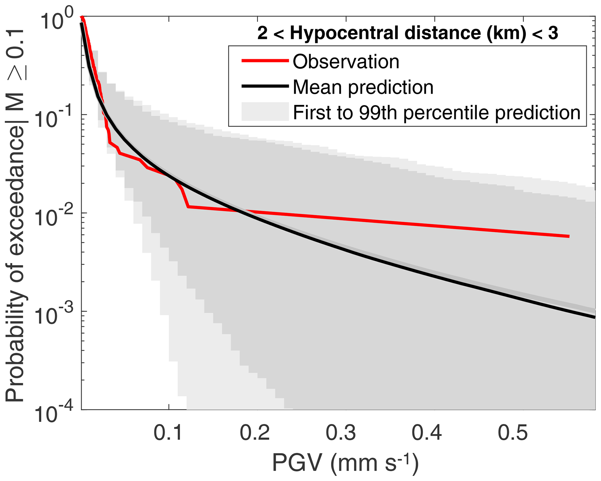
Figure 7Validating the assumption of spatial correlation in the ground motions of the case study: comparing predicted ground shaking with observed ground motion amplitudes. Also shown in dark grey are the mean (solid line) and first to 99th percentile predictions (shaded area) for the base (uncorrelated) case.
5.5 Different GMPE
The Cremen et al. (2019b) GMPE used in our assessment was specifically fit using data observed during both hydraulic fracturing operations at PNR and is therefore a particularly appropriate choice of ground motion model for the risk calculations of interest. On the other hand, pre-planning hazard calculations for PNR (Arup, 2014) employed the hypocentral distance model of Akkar et al. (2014) for predicting ground motion amplitudes, which is intended for application to crustal seismicity with much larger magnitudes than those that actually occurred at the site (Mw>4). As expected for extrapolation of a GMPE to smaller magnitudes (e.g. Bommer et al., 2007), this equation was consequently found to significantly overpredict the resulting ground motions (Cremen et al., 2019a, b). We examine the effect on the risk calculations of using this GMPE instead, which requires the Cremen et al. (2019b) GMPE to be substituted for the Akkar et al. (2014) equation in steps 3 and 4 of the procedure in Sect. 3.3. We assume a Vs30 value of 200 m s−1 for the GMPE, in line with Arup (2014).
5.6 Impacts of modelling assumptions
Figure 9 highlights the impact of the alternative modelling assumptions on the probability of exceeding PGV at least once in the exposure model, for specific volumes of injected fluid. Panels (b), (d), and (f) (right-hand side) present the ratio of the risk curves in the corresponding left-hand panel. For a given value of PGV, this ratio may be calculated as follows:
where Qi is the value of the risk curve for the ith alternative modelling assumption and Qb is its value in the base case (i.e. the original modelling approach outlined in Sect. 3). The stability of the results in both plots of Fig. 9 were assessed by simulating 100 bootstrap samples of the event catalogues and their associated PGV values and then recomputing the values on the y axes. Transparent regions of the curves indicate low stability, where the bootstrapped y values have coefficients of variation greater than 0.5. The following discussion focuses on the stable portions of the results.
The effect of the assumptions varies across different tolerable risk thresholds and volumes of injected fluid. Assuming the van der Elst et al. (2016) approach to rupture behaviour and using the Akkar et al. (2014) GMPE have the largest effect on the calculations, with both assumptions resulting in significant increases to the risk by a factor of 10 or 100, as well as an extension in the number of tolerable risk thresholds exceeded for a given injection volume. The increase in risk observed by assuming the van der Elst et al. (2016) approach to rupture behaviour is explained by the fact that it leads to larger magnitudes than the base case approach, since it does not constrain the magnitudes of events in line with the volume of fluid injected. The impact of this assumption is most significant for larger volumes, where the effect of removing the magnitude cap becomes most pronounced. For example, the maximum, 99th percentile, and 95th percentile Mw>0 event simulated for the van der Elst et al. (2016) approach in the case of 50 000 m3 injected volume were Mw=4.6, Mw=1.7, and Mw=1.1, respectively, whereas the corresponding events simulated for the base case approach were Mw=2.5, Mw=1.5, and Mw=1.1 (see Fig. 8 for a comparison of the maximum magnitudes simulated using both source models). Using the Akkar et al. (2014) GMPE leads to increased risk because it overestimates the ground shaking at PNR and therefore leads to higher PGV estimates than the Cremen et al. (2019b) GMPE.
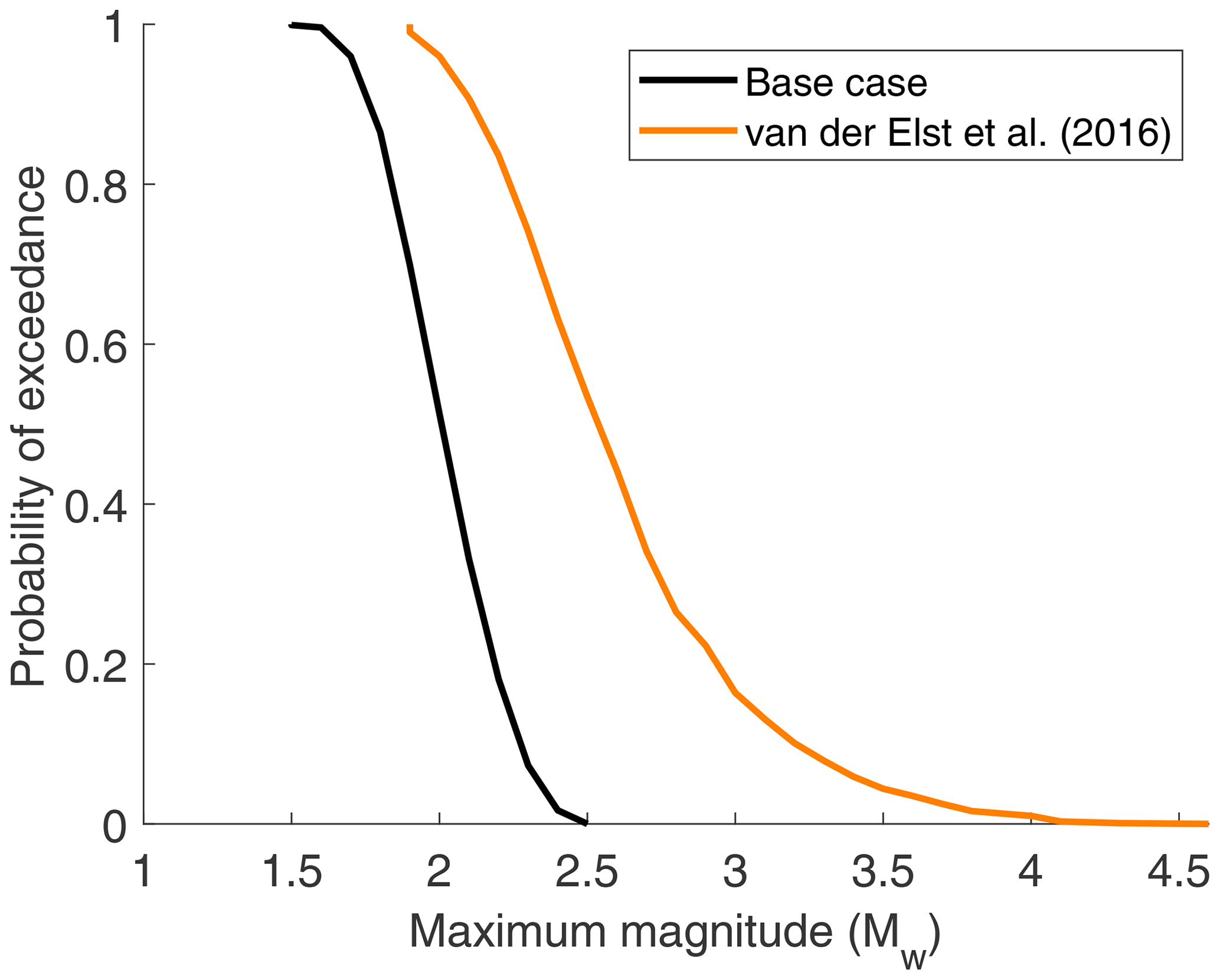
Figure 8Comparing the distribution of maximum magnitudes simulated using the base case approach to rupture behaviour (i.e. magnitudes are capped in proportion to volume injected) and that of van der Elst et al. (2016) (i.e. magnitudes follow a tectonic Gutenberg–Richter distribution), for 50 000 m3 injected volume.
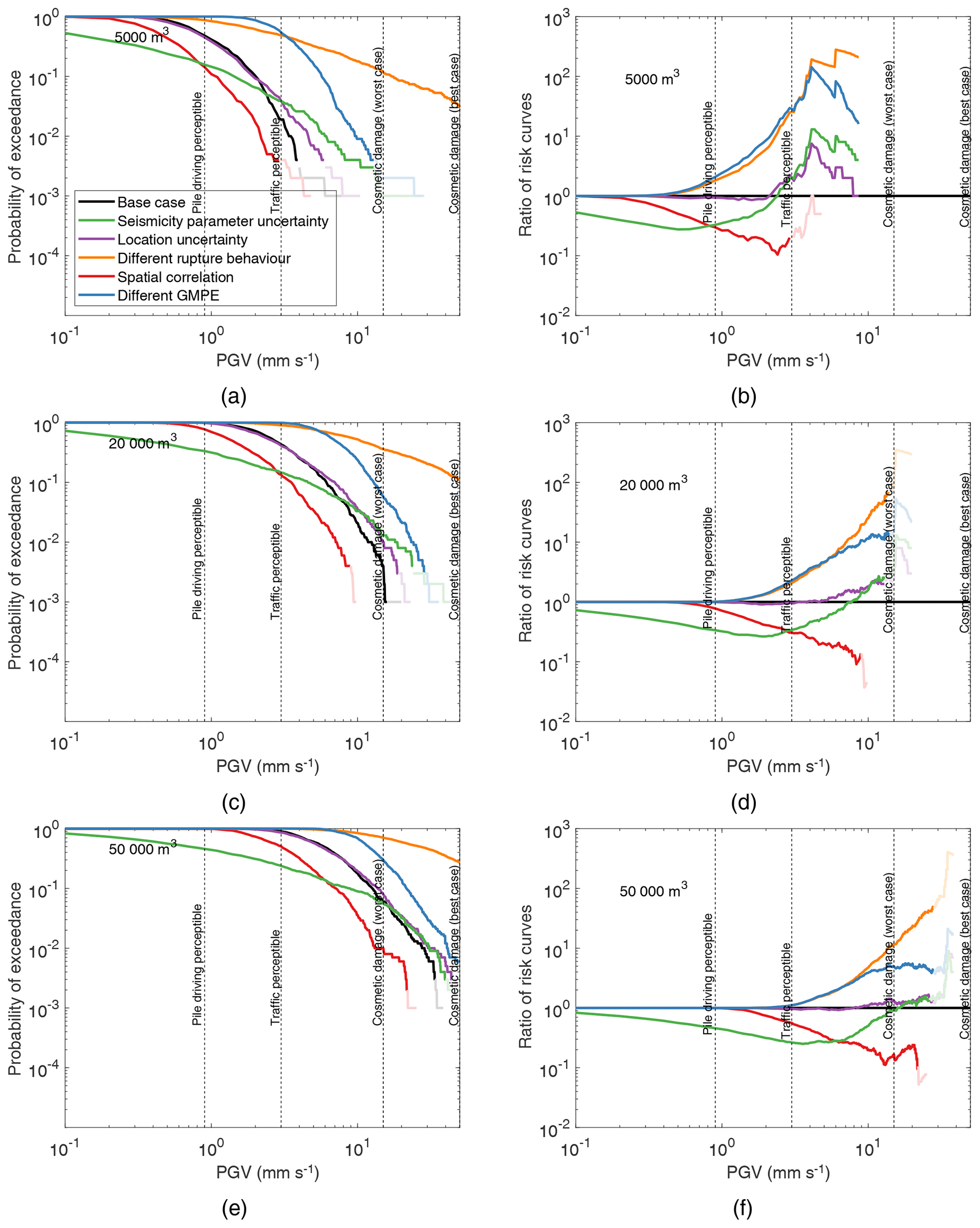
Figure 9Quantifying the impact of alternative modelling assumptions on the probability of exceeding various PGV levels at least once across all considered buildings in the exposure model.
Accounting for spatial correlation in the ground motions leads to lower probabilities of exceeding most tolerable risk thresholds, across all injection volumes examined. This finding is consistent with previous studies of the effect of spatial dependence on risk (e.g Weatherill et al., 2015). It is explained by the fact that spatial correlation widens the tails of the PGV distribution for a given event, such that small values have a higher probability of being sampled. Note that large PGV values also have a higher probability of being sampled in a spatially correlated portfolio, which should increase the chance of exceeding more severe risk thresholds. However, this is not observed for the exposure model of interest since the effect of spatial clustering (and therefore correlation) is most pronounced for the farthest distances examined (see Fig. 1).
Seismicity parameter uncertainty and location uncertainty lead to smaller probabilities of exceeding smaller PGV values and larger probabilities of exceeding higher PGV values. This implies that the probability distribution of potential ground shaking values widens for both assumptions, which is consistent with expectations for the introduction of uncertainty. The effect of seismicity parameter uncertainty is particularly notable for smaller PGV values. For example, it substantially underpredicts pile-driving exceedance probabilities relative to the base case where the parameters are known after the fact, which may pose a problem if this threshold is implemented in policies for managing the induced seismicity. Location uncertainty is the least impactful of all assumptions examined. It is most noticeable for larger PGV values and can lead to slight increases in the probabilities of exceeding the highest thresholds observed for a given injection volume.
The calculations of this section help to increase our understanding of the type of knowledge required to conduct an accurate risk assessment with the proposed framework. We have found that rupture behaviour and event locations are respectively the most and least important pieces of information to constrain for the calculations (at least in the case study of interest).
Based on the recommendations of a hydraulic fracturing review by the Royal Society (Mair et al., 2012), the UK Oil and Gas Authority has implemented a magnitude-based traffic light system (TLS) for the management of induced seismicity related to onshore shale gas development in the country. This TLS allows operations to continue as planned (“green light”) when the related induced seismicity is below ML=0, requires operations to proceed with caution (“amber light”) when the seismicity reaches ML=0 to ML=0.5, and stipulates a halt in operations (red light) when seismicity with ML≥0.5 occurs.
However, such magnitude-based systems have limited connection to the actual risks associated with the induced seismicity; it is instead the intensity of the ground motions (Bommer et al., 2015), in combination with an exposure model of the surrounding region (Lee et al., 2019), which determine the probability for nuisance or more damaging consequences. The results presented in Sect. 4.1 of this study could be used to design a more risk-orientated TLS for induced seismicity related to UK hydraulic fracturing, in which the magnitudes corresponding to each level of the system are chosen based on their potential to lead to ground motions that may cause nuisance consequences in the nearby area. For example, an amber light may correspond to the lowest magnitude for which there is a non-negligible probability of the pile-driving threshold being exceeded at any building (Mw≈1.2 for PNR from Sect. 4.1), and a red light may correspond to a magnitude just below that for which there is a non-negligible chance of cosmetic damage occurring at any building in a worst-case scenario (Mw≈2.1 for PNR). Similar approaches have been adopted for enhanced-geothermal-induced seismicity (e.g. Ader et al., 2020; Bommer et al., 2006; Häring et al., 2008), although our study has been informed by a more comprehensive analysis of the nearby exposure.
Alternatively, the proposed framework in Eq. (1) and the results of Sect. 4.2 could be used to design an injection-volume-based TLS for managing the risk associated with UK hydraulic-fracture-induced seismicity, where each level of the system corresponds to volumes of injected fluid with certain probabilities of causing ground motions that have nuisance potential. For example, an amber light could correspond to the first volume for which there is a non-negligible probability of the pile-driving threshold being exceeded, i.e. 1000 m3 for PNR from Sect. 4.2, which is roughly equivalent to a quarter of the actual volume injected during PNR-1z operations (Clarke et al., 2019), and a red light could correspond to a volume just less than that for which there is a non-negligible chance of cosmetic damage occurring in a worst-case scenario, i.e. 40 000 m3 for PNR, which is approximately equal to the planned injection volume for PNR-2 (Cuadrilla, 2019).
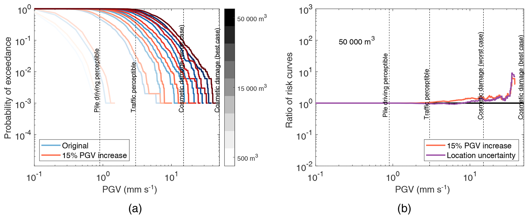
Figure 10Quantifying the impact of increasing PGV predictions by 15 % on the probability of exceeding various PGV levels at least once across all considered buildings in the exposure model, for the following injected volumes: 500, 1000, 5000, 10 000, 15 000, 20 000, 30 000, 40 000, and 50 000 m3.
A significant advantage of this approach over conventional magnitude- or ground-motion-based TLSs is that it is proactive rather than reactive, since the injection volume can be controlled ahead of time to avoid a red light ever occurring. The findings of Sect. 5 suggest that a notable amount of a priori information would be needed for such a system to perform accurately, however, particularly related to the rupture behaviour, the seismicity parameters (which can vary greatly even between stages), and the appropriate GMPE for modelling ground motions. The most effective means of implementing the proposed framework would therefore involve real-time updating of the seismicity forecast and the ground motion prediction based on a suite of preselected candidate models, following previously proposed approaches for EGS-related seismicity (e.g. Bachmann et al., 2011; Mena et al., 2013; Mignan et al., 2017; Broccardo et al., 2017).
7.1 Compatibility of GMPE predictions with vibration thresholds
Values of PGV predicted by a given GMPE may not be strictly compatible with the suggested nuisance vibration thresholds of the proposed framework. This is because GMPEs generally predict either horizontal or vertical amplitude, whereas the thresholds refer to the maximum amplitude across all three orthogonal components.
The Cremen et al. (2019b) GMPE used for the framework's application in Sect. 3 predicts horizontal PGV in terms of the geometric mean across both orthogonal directions. Previous work by Beyer and Bommer (2006) suggests that the maximum horizontal amplitude – which is expected to be the maximum of all three components (e.g. Ghofrani and Atkinson, 2014) – is 15 % larger than this value on average. We now investigate the implications on the risk calculations of the expected discrepancy between the GMPE ground shaking amplitudes and the maximum amplitudes. Maximum amplitudes are obtained by scaling the simulated ground motion intensities of step 4 in the Monte Carlo procedure (Sect. 3.3) by 1.15.
Figure 10a compares the probability of exceeding PGV values for ground shaking predicted by the GMPE (blue lines) and the equivalent maximum expected amplitude (red lines), across various injection volumes: 500, 1000, 5000, 10 000, 15 000, 20 000, 30 000, 40 000, and 50 000 m3. It is seen that differences between the two sets of curves are negligible. Figure 10b plots, for 50 000 m3 injected volume, the ratio of the risk curve for the maximum shaking amplitude to that for the shaking predicted by the GMPE (Eq. 10) and compares it to the equivalent ratio obtained for location uncertainty in Fig. 9, which was found to have the least impact on the risk calculations in Sect. 5. The two sets of ratios are broadly in line across the PGV values examined, which further confirms the insignificant effect of substituting the GMPE's ground shaking predictions with the maximum ground motion amplitudes expected. We therefore conclude that while there is a discrepancy between the velocities predicted by the GMPE and the definitions of the nuisance risk thresholds implemented, it does not have a significant impact on the risk calculations for the case study of interest.
7.2 Adequacy of source model assumption
This study has assumed that the rate of earthquakes during hydraulic fracturing is related to the volume of injected fluid, which has two main limitations: (1) there is no explicit temporal description of seismicity; i.e. the time period of event occurrence is not considered, and (2) the relationship only applies during the fluid injection phase, such that additional models are needed to describe post-injection seismicity, e.g. the decay law proposed by Langenbruch and Shapiro (2010). Many other types of forecast models have been proposed in the literature for injection-induced seismicity that may be more suitable for modelling earthquake occurrence in our case. These include models in which seismicity is instead proportional to the injection rate (e.g. Gischig and Wiemer, 2013) and so-called epidemic-type aftershock sequence (ETAS) models (e.g. Hainzl and Ogata, 2005). Evaluating the performance of various forecast models is outside the scope of this work. The proposed risk framework is capable of incorporating different types of source models in future studies if necessary however, by appropriately substituting the “Vt” term in Eq. (1).
This study has presented a novel framework for assessing some of the consequences of hydraulic-fracture-induced seismicity. The framework explicitly links the volume of fluid injected during operations to the risk of nuisance ground shaking, by combining statistical forecast models for injection-related seismicity, ground motion prediction equations for hydraulic fracturing, exposure models for affected regions, and suggested nuisance risk thresholds adopted from previous studies on human discomfort to vibrations.
We have demonstrated and validated the proposed modelling approach, using the UK Preston New Road (PNR) shale gas site and its surrounding area as a test bed. In particular, we showed how the framework can be used to determine event magnitudes and injection volumes for which prescribed nuisance risk thresholds may be exceeded at buildings near the site. For the specific case study examined, in which seismic events were deterministically located close to the surface projection of the PNR well stimulated in late 2018, we found that ground motions equivalent in amplitude to that at which pile driving becomes perceptible may be exceeded in the location of at least one building for event magnitudes exceeding the current UK induced seismicity traffic light system red light event (i.e. Mw=1.1), or injection volumes ≥ 1000 m3, while cosmetic damage may occur in at least one building for or injection volumes ≥ 40 000 m3.
We have also examined the sensitivity of the calculations to various modelling assumptions, to better understand the type of information required for conducting accurate risk assessments with the proposed framework. Implementing two different models for rupture behaviour (that both aligned reasonably well with observed source data) led to significantly varied risk estimates in particular. This work therefore highlights the importance of better understanding the physics to quantify likelihoods of different types of volume-related rupture, i.e. volume-capped moment release vs. seismicity that follows a tectonic Gutenberg–Richter distribution. Use of an appropriate GMPE is also essential for obtaining accurate risk estimates. On the other hand, we found that constraining event locations would not have a significant effect on the calculations (at least for the test bed considered in this study).
Finally, we discussed ways in which the proposed modelling approach could contribute to developing risk-informed policies for the management of induced seismicity related to UK shale gas development. For example, we suggested that the framework could be used to design an injection-volume-based traffic light system for induced seismicity based on real-time updating of the model parameters, which would enable injection volumes to be controlled ahead of time to mitigate the probabilities of causing ground motions with nuisance risk potential. This proactive system could replace the reactive magnitude-based traffic light system currently used in the UK, in which the thresholds do not explicitly account for the associated risks. We expect the findings of this study to be helpful as a decision support tool for stakeholders involved in the regulation of shale gas development in the UK.
No new data were created as part of this study. Fluid injection volumes at the PNR-1z well and some related seismicity data were respectively obtained from the “Pumping Data” and “Microseismic” sections of the UK Oil and Gas Authority's database on PNR operations (https://www.ogauthority.co.uk/exploration-production/onshore/onshore-reports-and-data/preston-new-road-pnr-1z-hydraulic-fracturing-operations-data/, last access: September 2020) (UK Oil & Gas Authority, 2020). Additional PNR-1z and all PNR-2 seismicity data were retrieved from the BGS earthquake database (http://www.earthquakes.bgs.ac.uk/earthquakes/dataSearch.html, last access: December 2019) (British Geological Survey, 2019b). Some ground motion information for PNR-1z seismicity was obtained from the “Waveform Data” portal of the BGS data archive (ftp://seiswav.bgs.ac.uk/, last access: September 2020) (British Geological Survey, 2020). The remaining ground motion data used are available from the UK Oil and Gas Authority on request. Building data were acquired from OS mapping, accessed through the Edina Digimap service (Morris et al., 2000). All other underlying data to support the conclusions are provided in this paper. Code used in this research is available from the authors on request.
Both authors conceived and designed the research. GC drafted the written content of the manuscript, which both authors reviewed. GC performed the calculations. Both authors developed the figures.
The authors declare that they have no conflict of interest.
The authors are grateful to the UK Oil and Gas Authority and the British Geological Survey for making necessary data available. The authors thank James Verdon and Tom Kettlety (University of Bristol) for helpful feedback on seismicity source modelling. They thank Brian Baptie (BGS) and Antony Butcher (University of Bristol) for fruitful discussions on the ground motion data. Finally, the authors acknowledge the constructive comments of the two anonymous reviewers that improved the quality of this manuscript.
This work has been funded by the Natural Environment Research Council (NERC; grant no. NE/R017956/1) “Evaluation, Quantification and Identification of Pathways and Targets for the assessment of Shale Gas RISK (EQUIPT4RISK)” and the Bristol University Microseismic Projects (BUMPS).
This paper was edited by Filippos Vallianatos and reviewed by two anonymous referees.
Ader, T., Chendorain, M., Free, M., Saarno, T., Heikkinen, P., Malin, P. E., Leary, P., Kwiatek, G., Dresen, G., Bluemle, F., and Vuorinen, T.: Design and implementation of a traffic light system for deep geothermal well stimulation in Finland, J. Seismol., 24, 991–1014, 2020. a, b, c
Akkar, S., Sandıkkaya, M., and Bommer, J.: Empirical ground-motion models for point-and extended-source crustal earthquake scenarios in Europe and the Middle East, B. Earthq. Eng., 12, 359–387, 2014. a, b, c, d
Arup: Temporary shale gas exploration, Environmental Statement, Preston New Road, Lancashire, 2014. a, b
Assatourians, K. and Atkinson, G. M.: EqHaz: An open-source probabilistic seismic-hazard code based on the Monte Carlo simulation approach, Seismol. Res. Lett., 84, 516–524, 2013. a
Athanasopoulos, G. and Pelekis, P.: Ground vibrations from sheetpile driving in urban environment: measurements, analysis and effects on buildings and occupants, Soil Dynam. Earthq. Eng., 19, 371–387, 2000. a
Atkinson, G. M., Eaton, D. W., Ghofrani, H., Walker, D., Cheadle, B., Schultz, R., Shcherbakov, R., Tiampo, K., Gu, J., Harrington, R. M., Liu, Y., van der Baan, M., and Kao, H.: Hydraulic fracturing and seismicity in the western Canada sedimentary basin, Seismol. Res. Lett., 87, 631–647, 2016. a
Atkinson, G. M., Eaton, D. W., and Igonin, N.: Developments in understanding seismicity triggered by hydraulic fracturing, Nat. Rev. Earth Environ., 1, 264–277, 2020. a
Bachmann, C. E., Wiemer, S., Woessner, J., and Hainzl, S.: Statistical analysis of the induced Basel 2006 earthquake sequence: introducing a probability-based monitoring approach for Enhanced Geothermal Systems, Geophys. J. Int., 186, 793–807, 2011. a
Bao, X. and Eaton, D. W.: Fault activation by hydraulic fracturing in western Canada, Science, 354, 1406–1409, 2016. a
Baptie, B.: Earthquake Seismology 2018/2019, British Geological Survey Open Report OR/19/039, British Geological Survey, Edinburgh, UK, 2019. a, b
Barneich, J.: Vehicle induced ground motion, in: Vibration Problems in Geotechnical Engineering, edited by: Gazetas, G. and Selig, E., Proceedings of Symposium Held by the Geotechnical Engineering Division in conjunction with the ASCE Convention, 22 October 1985, Detroit, MI, USA, 187–202, 1985. a
Bazzurro, P. and Allin Cornell, C.: Disaggregation of seismic hazard, B. Seismol. Soc. Am., 89, 501–520, 1999. a
Beyer, K. and Bommer, J. J.: Relationships between median values and between aleatory variabilities for different definitions of the horizontal component of motion, B. Seismol. Soc. Am., 96, 1512–1522, 2006. a
Bommer, J. J. and Alarcon, J. E.: The prediction and use of peak ground velocity, J. Earthq. Eng., 10, 1–31, 2006. a
Bommer, J. J., Oates, S., Cepeda, J. M., Lindholm, C., Bird, J., Torres, R., Marroquin, G., and Rivas, J.: Control of hazard due to seismicity induced by a hot fractured rock geothermal project, Eng. Geol., 83, 287–306, 2006. a, b, c
Bommer, J. J., Stafford, P. J., Alarcón, J. E., and Akkar, S.: The influence of magnitude range on empirical ground-motion prediction, B. Seismol. Soc. Am., 97, 2152–2170, 2007. a
Bommer, J. J., Crowley, H., and Pinho, R.: A risk-mitigation approach to the management of induced seismicity, J. Seismol., 19, 623–646, 2015. a, b, c, d
Boore, D. M., Gibbs, J. F., Joyner, W. B., Tinsley, J. C., and Ponti, D. J.: Estimated ground motion from the 1994 Northridge, California, earthquake at the site of the Interstate 10 and La Cienega Boulevard bridge collapse, West Los Angeles, California, B. Seismol. Soc. Am., 93, 2737–2751, 2003. a
Bourne, S., Oates, S., Bommer, J., Dost, B., Van Elk, J., and Doornhof, D.: A Monte Carlo method for probabilistic hazard assessment of induced seismicity due to conventional natural gas production, B. Seismol. Soc. Am., 105, 1721–1738, 2015. a, b, c
British Geological Survey: Statement on seismic activity at Preston New Road, Lancashire on 28/8/19, available at: https://www.bgs.ac.uk/news/docs/BGS Statement on seismic_activity_28_8_19.pdf (last access: March 2020), 2019a. a
British Geological Survey: BGS earthquake database search, available at: http://www.earthquakes.bgs.ac.uk/earthquakes/dataSearch.html (last access: December 2019), 2019b. a
British Geological Survey: BGS ftp site, available at: ftp://seiswav.bgs.ac.uk/, last access: September 2020. a
Broccardo, M., Mignan, A., Wiemer, S., Stojadinovic, B., and Giardini, D.: Hierarchical Bayesian Modeling of Fluid-Induced Seismicity, Geophys. Res. Lett., 44, 11–357, 2017. a
BSI: Evaluation and measurement for vibration in buildings: Guide to damage levels from groundborne vibration, BS7385-2, British Standards Institute, London, UK, 1993. a, b
Butcher, A., Luckett, R., Kendall, J.-M., and Baptie, B.: Seismic Magnitudes, Corner Frequencies, and Microseismicity: Using Ambient Noise to Correct for High‐Frequency Attenuation, B. Seismol. Soc. Am., 110, 1260–1275, https://doi.org/10.1785/0120190032, 2019. a
Chen, H., Meng, X., Niu, F., Tang, Y., Yin, C., and Wu, F.: Microseismic monitoring of stimulating shale gas reservoir in SW China: 2. Spatial clustering controlled by the preexisting faults and fractures, J. Geophys. Res.-Solid, 123, 1659–1672, 2018. a
Clarke, H., Eisner, L., Styles, P., and Turner, P.: Felt seismicity associated with shale gas hydraulic fracturing: The first documented example in Europe, Geophys. Res. Lett., 41, 8308–8314, 2014. a, b
Clarke, H., Verdon, J. P., Kettlety, T., Baird, A., and Kendall, J.-M.: Real-time imaging, forecasting, and management of human-induced seismicity at Preston New Road, Lancashire, England, Seismol. Res. Lett., 90, 1902–1915, 2019. a, b, c, d, e, f, g, h, i, j, k
Cornell, C. A.: Engineering seismic risk analysis, B. Seismol. Soc. Am., 58, 1583–1606, 1968. a
Cotton, M., Rattle, I., and Van Alstine, J.: Shale gas policy in the United Kingdom: An argumentative discourse analysis, Energ. Policy, 73, 427–438, 2014. a
Cremen, G., Werner, M. J., and Baptie, B.: Understanding induced seismicity hazard related to shale gas exploration in the UK, in: SECED 2019 Conference: Earthquake Risk and Engineering towards a Resilient World, September 2019, London, UK, 2019a. a, b, c
Cremen, G., Werner, M. J., and Baptie, B.: A New Procedure for Evaluating Ground-Motion Models, with Application to Hydraulic-Fracture-Induced Seismicity in the United Kingdom, B. Seismol. Soc. Am., 110, 2380–2397, https://doi.org/10.1785/0120190238, 2019b. a, b, c, d, e, f, g, h, i, j, k, l, m, n
Crowley, H., Pinho, R., van Elk, J., and Uilenreef, J.: Probabilistic damage assessment of buildings due to induced seismicity, B. Earthq. Eng., 17, 4495–4516, 2018. a
Cuadrilla: Preston New Road 1z Hydraulic Fracture Plan, Cuadrilla Resources Ltd., Bamber Bridge, Preston, UK, 2017. a, b, c, d
Cuadrilla: Hydraulic Fracture Plan PNR 2, Cuadrilla Resources Ltd., Bamber Bridge, Preston, UK, 2019. a, b
Davies, R., Foulger, G., Bindley, A., and Styles, P.: Induced seismicity and hydraulic fracturing for the recovery of hydrocarbons, Mar. Petrol. Geol., 45, 171–185, 2013. a
De Pater, C. and Baisch, S.: Geomechanical study of Bowland Shale seismicity, Synthesis report, Cuadrilla Resources Ltd., Lichfield, Staffordshire, UK, 57 pp., 2011. a
Douglas, J. and Aochi, H.: Using estimated risk to develop stimulation strategies for enhanced geothermal systems, Pure Appl. Geophys., 171, 1847–1858, 2014. a
Douglas, J., Edwards, B., Convertito, V., Sharma, N., Tramelli, A., Kraaijpoel, D., Cabrera, B. M., Maercklin, N., and Troise, C.: Predicting ground motion from induced earthquakes in geothermal areas, B. Seismol. Soc. Am., 103, 1875–1897, 2013. a, b
Eaton, D. W., Davidsen, J., Pedersen, P. K., and Boroumand, N.: Breakdown of the Gutenberg-Richter relation for microearthquakes induced by hydraulic fracturing: Influence of stratabound fractures, Geophys. Prospect., 62, 806–818, 2014. a
Ellsworth, W. L.: Injection-induced earthquakes, Science, 341, 1225942, https://doi.org/10.1126/science.1225942, 2013. a
Esposito, S. and Iervolino, I.: Spatial correlation of spectral acceleration in European data, B. Seismol. Soc. Am., 102, 2781–2788, 2012. a, b
Foulger, G. R., Wilson, M. P., Gluyas, J. G., Julian, B. R., and Davies, R. J.: Global review of human-induced earthquakes, Earth-Sci. Rev., 178, 438–514, 2018. a, b
Gallegos, T. J., Varela, B. A., Haines, S. S., and Engle, M. A.: Hydraulic fracturing water use variability in the United States and potential environmental implications, Water Resour. Res., 51, 5839–5845, 2015. a
Ghofrani, H. and Atkinson, G. M.: Site condition evaluation using horizontal-to-vertical response spectral ratios of earthquakes in the NGA-West 2 and Japanese databases, Soil Dynam. Earthq. Eng., 67, 30–43, 2014. a
Giardini, D.: Geothermal quake risks must be faced, Nature, 462, 848–849, 2009. a, b
Gischig, V. S.: Rupture propagation behavior and the largest possible earthquake induced by fluid injection into deep reservoirs, Geophys. Res. Lett., 42, 7420–7428, 2015. a
Gischig, V. S. and Wiemer, S.: A stochastic model for induced seismicity based on non-linear pressure diffusion and irreversible permeability enhancement, Geophys. J. Int., 194, 1229–1249, 2013. a
Ground Water Protection Council: Modern shale gas development in the United States: A primer, US Department of Energy, Office of Fossil Energy, Washington, D.C., USA, 2009. a
Grünthal, G.: European macroseismic scale 1998, Tech. rep., European Seismological Commission (ESC), Luxembourg, 1998. a
Gupta, A. and Baker, J. W.: A framework for time-varying induced seismicity risk assessment, with application in Oklahoma, B. Earthq. Eng., 17, 4475–4493, 2019. a
Hainzl, S. and Ogata, Y.: Detecting fluid signals in seismicity data through statistical earthquake modeling, J. Geophys. Res.-Sol. Ea., 110, B05S07, https://doi.org/10.1029/2004JB003247, 2005. a
Hallo, M., Eisner, L., and Ali, M.: Expected level of seismic activity caused by volumetric changes, First Break, 30, 97–100, 2012. a, b
Hallo, M., Oprsal, I., Eisner, L., and Ali, M. Y.: Prediction of magnitude of the largest potentially induced seismic event, J. Seismol., 18, 421–431, 2014. a, b
Häring, M. O., Schanz, U., Ladner, F., and Dyer, B. C.: Characterisation of the Basel 1 enhanced geothermal system, Geothermics, 37, 469–495, 2008. a
Haylock, D.: Numeracy for teaching, Sage, London, UK, 2001. a
Jayaram, N. and Baker, J. W.: Statistical tests of the joint distribution of spectral acceleration values, B. Seismol. Soc. Am., 98, 2231–2243, 2008. a
Johnson, E. G. and Johnson, L. A.: Hydraulic fracture water usage in northeast British Columbia: locations, volumes and trends, in: Geoscience Reports 2012, British Columbia Ministry of Energy and Mines, Victoria, British Columbia, Canada, 41–63, 2012. a
Kettlety, T., Verdon, J., Werner, M., and Kendall, J.: Stress transfer from opening hydraulic fractures controls the distribution of induced seismicity, J. Geophys. Res.-Solid, 125, e2019JB018794, https://doi.org/10.1029/2019JB018794, 2020. a
Kraft, T., Mai, P. M., Wiemer, S., Deichmann, N., Ripperger, J., Kästli, P., Bachmann, C., Fäh, D., Wössner, J., and Giardini, D.: Enhanced geothermal systems: Mitigating risk in urban areas, Eos T. Am. Geophys. Un., 90, 273–274, 2009. a
Kwiatek, G., Saarno, T., Ader, T., Bluemle, F., Bohnhoff, M., Chendorain, M., Dresen, G., Heikkinen, P., Kukkonen, I., Leary, P., Leonhardt, M., Malin, P., Martínez-Garzón, P., Passmore, K., Passmore, P., Valenzuela, S., and Wollin, C.: Controlling fluid-induced seismicity during a 6.1-km-deep geothermal stimulation in Finland, Sci. Adv., 5, eaav7224, https://doi.org/10.1126/sciadv.aav7224, 2019. a
Langenbruch, C. and Shapiro, S. A.: Decay rate of fluid-induced seismicity after termination of reservoir stimulations, Geophysics, 75, MA53–MA62, 2010. a
Lee, K.-K., Ellsworth, W. L., Giardini, D., Townend, J., Ge, S., Shimamoto, T., Yeo, I.-W., Kang, T.-S., Rhie, J., Sheen, D.-H., Chang, C., Woo, J.-U., and Langenbruch, C.: Managing injection-induced seismic risks, Science, 364, 730–732, 2019. a, b
MacRae, G. A.: Decision making tools for seismic risk, in: vol. 28, Proceedings of the New Zealand Society of Earthquake Engineering Annual Conference Paper, March 2006, Napier, New Zealand, 2006. a
Mair, R., Bickle, M., Goodman, D., Koppelman, B., Roberts, J., Selley, R., Shipton, Z., Thomas, H., Walker, A., Woods, E., et al.: Shale gas extraction in the UK: a review of hydraulic fracturing, Royal Society and Royal Academy of Engineering, London, UK, 2012. a, b
Mancini, S., Segou, M., Werner, M. J., and Baptie, B. J.: Statistical modelling of the Preston New Road seismicity: Towards probabilistic forecasting tools, Report No. CR/19/068 Commissioned by the Oil and Gas Authority, available at: https://www.ogauthority.co.uk/media/6147/bgs-innovations-in-forecasting.pdf (last access: September 2020), 2019. a, b
McGarr, A.: Maximum magnitude earthquakes induced by fluid injection, J. Geophys. Res.-Solid, 119, 1008–1019, 2014. a
Mena, B., Wiemer, S., and Bachmann, C.: Building robust models to forecast the induced seismicity related to geothermal reservoir enhancement, B. Seismol. Soc. Am., 103, 383–393, 2013. a
Mignan, A., Broccardo, M., Wiemer, S., and Giardini, D.: Induced seismicity closed-form traffic light system for actuarial decision-making during deep fluid injections, Sci. Rep.-UK, 7, 13607, https://doi.org/10.1038/s41598-017-13585-9, 2017. a, b
Mignan, A., Karvounis, D., Broccardo, M., Wiemer, S., and Giardini, D.: Including seismic risk mitigation measures into the Levelized Cost of Electricity in enhanced geothermal systems for optimal siting, Appl. Energ., 238, 831–850, 2019. a
Morris, B., Medyckyj-Scott, D., and Burnhill, P.: EDINA Digimap: new developments in the Internet Mapping and Data Service for the UK Higher Education community, Liber Quart., 10, 445–453, 2000. a
Musson, R.: Determination of design earthquakes in seismic hazard analysis through Monte Carlo simulation, J. Earthq. Eng., 3, 463–474, 1999. a
Park, J., Bazzurro, P., and Baker, J. W.: Modeling spatial correlation of ground motion intensity measures for regional seismic hazard and portfolio loss estimation, in: 10th International Conference on Application of Statistic and Probability in Civil Engineering (ICASP10), Tokyo, Japan, 8 pp., 2007. a
Precht, P. and Dempster, D.: Jurisdictional review of hydraulic fracturing regulation, Final report for Nova Scotia Hydraulic Fracturing Review Committee, Nova Scotia Department of Energy and Nova Scotia Environment, available at: https://novascotia.ca/nse/pollutionprevention/docs/Consultation.Hydraulic.Fracturing-Jurisdictional.Review.pdf (last access: September 2020), 2012. a
Scasserra, G., Stewart, J. P., Bazzurro, P., Lanzo, G., and Mollaioli, F.: A comparison of NGA ground-motion prediction equations to Italian data, B. Seismol. Soc. Am., 99, 2961–2978, 2009. a
Shapiro, S. A., Dinske, C., Langenbruch, C., and Wenzel, F.: Seismogenic index and magnitude probability of earthquakes induced during reservoir fluid stimulations, Leading Edge, 29, 304–309, 2010. a
Third Energy: Hydraulic Fracture Plan for well KM-8, Third Energy UK Gas Ltd., Malton, North Yorkshire, UK, 2017. a
UK Oil & Gas Authority: Preston New Road – PNR 1Z – Hydraulic Fracturing Operations Data, available at: https://www.ogauthority.co.uk/exploration-production/onshore/onshore-reports-and-data/preston-new-road-pnr-1z-hydraulic-fracturing-operations-data/, last access: September 2020. a
van der Elst, N. J., Page, M. T., Weiser, D. A., Goebel, T. H., and Hosseini, S. M.: Induced earthquake magnitudes are as large as (statistically) expected, J. Geophys. Res.-Solid, 121, 4575–4590, 2016. a, b, c, d, e, f, g, h
Van Eck, T., Goutbeek, F., Haak, H., and Dost, B.: Seismic hazard due to small-magnitude, shallow-source, induced earthquakes in The Netherlands, Eng. Geol., 87, 105–121, 2006. a
Verdon, J. P. and Budge, J.: Examining the capability of statistical models to mitigate induced seismicity during hydraulic fracturing of shale gas reservoirs, B. Seismol. Soc. Am., 108, 690–701, 2018. a, b
Verdon, J. P., Baptie, B. J., and Bommer, J. J.: An improved framework for discriminating seismicity induced by industrial activities from natural earthquakes, Seismol. Res. Lett., 90, 1592–1611, https://doi.org/10.1785/0220190030, 2019. a
Walters, R. J., Zoback, M. D., Baker, J. W., and Beroza, G. C.: Characterizing and responding to seismic risk associated with earthquakes potentially triggered by fluid disposal and hydraulic fracturing, Seismol. Res. Lett., 86, 1110–1118, 2015. a, b
Wang, M. and Takada, T.: Macrospatial correlation model of seismic ground motions, Earthq. Spectra, 21, 1137–1156, 2005. a
Weatherill, G., Silva, V., Crowley, H., and Bazzurro, P.: Exploring the impact of spatial correlations and uncertainties for portfolio analysis in probabilistic seismic loss estimation, B. Earthq. Eng., 13, 957–981, 2015. a
Westaway, R.: The importance of characterizing uncertainty in controversial geoscience applications: induced seismicity associated with hydraulic fracturing for shale gas in northwest England, P. Geologist. Assoc., 127, 1–17, 2016. a
Whitmarsh, L., Nash, N., Upham, P., Lloyd, A., Verdon, J. P., and Kendall, J.-M.: UK public perceptions of shale gas hydraulic fracturing: The role of audience, message and contextual factors on risk perceptions and policy support, Appl. Energ., 160, 419–430, 2015. a
Williams, L., Macnaghten, P., Davies, R., and Curtis, S.: Framing `fracking': Exploring public perceptions of hydraulic fracturing in the United Kingdom, Publ.Underst. Sci., 26, 89–104, 2017. a
Woessner, J., Laurentiu, D., Giardini, D., Crowley, H., Cotton, F., Grünthal, G., Valensise, G., Arvidsson, R., Basili, R., Demircioglu, M. B., Hiemer, S., Meletti, C., Musson, R. W., Rovida, A. N., Sesetyan, K., Stucchi, M., and The SHARE Consortium: The 2013 European seismic hazard model: key components and results, B. Earthq. Eng., 13, 3553–3596, 2015. a
- Abstract
- Introduction
- Framework outline
- Case study framework application
- Case study results
- Exploring the impacts of modelling assumptions
- Implications for future policy design
- Possible limitations
- Conclusions
- Code and data availability
- Author contributions
- Competing interests
- Acknowledgements
- Financial support
- Review statement
- References