Brief communication: The role of using precipitation or river discharge data when assessing global coastal compound flooding

Interacting storm surges and high water runoff can cause compound flooding (CF) in low-lying coasts and river estuaries. The large-scale CF hazard has been typically studied using proxies such as the concurrence of storm surge extremes either with precipitation or with river discharge extremes. Here the impact of the choice of such proxies is addressed employing state-of-the-art global datasets. Although they are proxies of diverse physical mechanisms, we find that the two approaches show similar CF spatial patterns. On average, deviations are smaller in regions where assessing the actual CF is more relevant, i.e. where the CF potential is high. Differences between the two assessments increase with the catchment size, and our findings indicate that CF in long rivers (catchment ≳5–10×10³ km²) should be analysed using river discharge data. The precipitation-based assessment allows for considering local-rainfall-driven CF and CF in small rivers not resolved by large-scale datasets.

1 Introduction

Compound flooding (CF) happens in low-lying coastal areas due to the interaction of high precipitation runoff and high sea level. The combination of the two hazards can cause larger damages than those caused by either of the hazards in isolation, and recent events have occurred in e.g. Mozambique (2019), Texas (USA, 2017), the Shoalhaven estuary (Australia, 2016), Ravenna (Italy, 2015), Cork (Ireland, 2009), and Lymington (UK, 1999) (Couasnon et al., 2020; Zscheischler et al., 2018; Kumbier et al., 2018; Bevacqua et al., 2017; Olbert et al., 2017; Hendry et al., 2019). Practitioners and the scientific community are becoming more aware of CF risk, and there were several recent studies addressing the phenomenon at local (Bevacqua et al., 2017; Kumbier et al., 2018; van den Hurk et al., 2015; Ridder et al., 2018) or larger scales (Wahl et al., 2015; Bevacqua et al., 2019; Couasnon et al., 2020; Ward et al., 2018; Ganguli and Merz, 2019a, b; Wu and Leonard, 2019; Wu et al., 2018; Moftakhari et al., 2017). Recent advances in large-scale sea level and river discharge modelling allowed for the generation of sub-daily time series of water levels along the global coastline (Vousdoukas et al., 2018; Muis et al., 2016), thus enabling continental CF assessments (Ward et al., 2018; Bevacqua et al., 2019; Couasnon et al., 2020).

CF can be the result of different mechanisms depending on the local topography and meteorology. According to Wahl et al. (2015), CF is possible to occur when (1) the joint occurrence of high river discharge and storm surge in estuarine regions may elevate water levels to a point where flooding is initiated or its impacts are exacerbated; (2) a destructive storm surge, which already caused widespread flooding, is followed by rainfall, as the latter can drive additional flooding, even if it is not an extreme event on its own; and (3) a moderate storm surge occurs which does not directly cause flooding but is high enough to fully block or slow down gravity-fed storm water drainage, and as a result precipitation causes flooding. In addition, CF may occur if (4) precipitation falls on wet soil that is saturated by a preceding storm surge (Bevacqua et al., 2019).

Quantifying the actual CF, i.e. the water level resulting from the combination of pluvial or fluvial flooding and high sea level, is challenging. For example, quantifying and interpreting CF in the vicinity of rivers (mechanism 1) requires water level measurements in the river mouth, which are rare, probably because most gauges are installed to monitor either riverine or marine processes (Bevacqua et al., 2017; Paprotny et al., 2018). Model-based data are also limited because only recently have modellers started considering CF. Statistical and hydrodynamic modelling approaches integrating fluvial and sea level flooding have been developed and applied recently at the local scale (Bevacqua et al., 2017; van den Hurk et al., 2015; Kumbier et al., 2018; Khanal et al., 2019); however, at a large scale, these approaches are only now being developed. Similarly, the explicit study of the actual CF water level due to pluvial flooding and storm surges (mechanisms 2-4) has not received much attention so far, to our knowledge, which may also be due to the scarcity of data. Thus, to gain information on the CF hazard at the regional, continental, or global scales, scientists usually employ proxies of flood hazard, e.g. the probability of potential CF (Bevacqua et al., 2019; Ward et al., 2018; Wahl et al., 2015; Couasnon et al., 2020; Paprotny et al., 2018). Quantifying potential CF, under the present or future climate, is useful, as it allows for identifying potential hotspots of CF hazard. Then, more detailed assessments of the local CF risk can be carried out at such hotspots, using computationally intensive methodologies that integrate all the hydrological and meteorological sources of flooding and their physical interaction (Wahl et al., 2015).

The large-scale assessment of potential CF includes the analysis of the probability (or return periods) of concurring extreme values of CF drivers. Two main approaches exist, focussing, respectively, on the analysis of the probability of concurring high values of sea level and river discharge or of sea level and precipitation. Through considering river discharge, the first approach takes into account CF in estuaries and deltas, i.e. serving as a proxy of CF mechanism 1. The second approach, based on the analysis of accumulated precipitation around the coast when the high sea levels occur, can represent CF due to local precipitation extremes, i.e. related to mechanisms 2, 3, and 4. Given that precipitation is among the main drivers of river discharge, the two proxies are correlated to a certain extent, and the use of precipitation can thereby allow for quantifying CF potential also in certain river estuaries. However, the correlation between the two proxies can be sometimes poor, especially in locations where river discharge is strongly influenced by other factors such as snowmelt, evaporation, and accumulated precipitation over previous weeks or months (Blöschl et al., 2019).

Given the scarcity and heterogeneous distribution of in situ data (Ward et al., 2018; Couasnon et al., 2020; Wu et al., 2018), scientists have started to employ model data – of river discharge, storm surge, and precipitation – to assess the large-scale potential CF hazard (Ward et al., 2018; Bevacqua et al., 2019; Wu et al., 2018; Couasnon et al., 2020; Wu et al., 2018; Paprotny et al., 2018; Bevacqua et al., 2020). Against the foregoing background, the present study aims to assess whether a precipitation-based large-scale CF assessment can be used as a surrogate for potential CF in estuaries at the large-scale. To that end we use coherent global model datasets of storms surges (including wave effects; Vousdoukas et al., 2018), precipitation (Beck et al., 2017b), and river discharge (Couasnon et al., 2020; Eilander, 2019) and conduct a first global comparison of the results obtained through the two approaches, keeping all the other methodological aspects identical.

2 Data

We analyse the period 1979–2015. We consider river discharge daily maxima from a publicly available global dataset (Eilander, 2019; Couasnon et al., 2020), which includes coastal catchments larger than 1000 km². The dataset was the result of hydrological model simulations forced with temperature and potential evaporation derived from ERA-Interim (European Centre for Medium-Range Weather Forecasts Reanalysis) and with precipitation from the MSWEPv1.2 dataset (Multi-Source Weighted-Ensemble Precipitation; Couasnon et al., 2020). The latter is obtained by merging gauge, satellite, and reanalysis data (including ERA-Interim); more information can be found in Beck et al. (2017b).

Precipitation is taken from the same MSWEPv1.2 dataset used to simulated river discharges and consists of daily data over a 0.25^∘ grid. On each day we consider accumulated precipitation amounts within a 3 d centred window. This enables us to account for precipitation occurring just before and after midnight of the storm surge day (Bevacqua et al., 2019; Martius et al., 2016) and to consider different mechanisms causing CF (Wahl et al., 2015; Bevacqua et al., 2019).

Storm surges and waves were simulated with the hydrodynamic model D-Flow Flexible Mesh (D-Flow FM; Vousdoukas et al., 2017, 2018) and the wave model Wavewatch III (Mentaschi et al., 2017; Vousdoukas et al., 2017, 2018). The wave model was forced by 6-hourly wind, while D-Flow FM was also forced by sea level pressure fields, both available from the ERA-Interim reanalysis (Dee et al., 2011). The effects of tropical cyclones (TCs) were considered in the reanalysis through storm surge simulations forced by downscaled atmospheric fields from all recorded TCs and by considering satellite-observed TC wave extremes (Vousdoukas et al., 2018). Astronomical tides are not considered in this analysis in order to focus on the meteorological component of the sea level, excluding the stochastic coupling with tide induced water level variations. We consider daily water level maxima from the combined result of storm surges and wave setup (hereinafter mentioned as storm surges) according to Vousdoukas et al. (2018).

We analyse CF only around river mouth locations whose nearest precipitation and storm surge grid points lie within a distance of 75 km (Couasnon et al., 2020). This results in considering locations at river mouths of catchments with a size of between about 1000 and 3 690 000 km² (95 % having a size smaller than 50 000 km²; Fig. 3f).

2.1 Methods

We assess the potential CF hazard via bivariate return periods of concurring extreme events (Vandenberghe et al., 2011; Manning et al., 2019) of the variables X and Y, i.e. storm surge and precipitation (CF_prec) or storm surge and river discharge (CF_river). Extremes of the individual variables (x_ext and y_ext) are defined as the associated α-year return levels. We use different α values in the following, though we present the main results for α=5; images for α=2 are shown in the Appendix. Return levels are obtained through fitting a generalised-extreme-value distribution to the annual maxima of the individual variables (Coles et al., 2001). Annual maxima are defined based on adjacent windows centred on the month where the climatological river discharge average is the highest, rather than from January–December windows (such a window definition reduces the chance of selecting two consecutive annual maxima belonging to the same river discharge extreme event and therefore leads to a more robust definition of the return levels). Overall, given the definition of the extremes based on α-year return levels, the bivariate return period is inherently linked to the dependence of the pairs in the tail of the distribution.

CF bivariate return periods are computed following the methodology presented by Bevacqua et al. (2019). The CF return period computation is based on the bivariate distribution of the variables of interest (X and Y), which is estimated semi-empirically to allow for robust estimation. For a given location, we select pairs whose individual values are simultaneously larger than the individual 95th percentiles (x_sel and y_sel), and we model these pairs via a copula-based distribution. If the defined thresholds result in a small group of selected pairs, we lower the 95th percentile selection threshold to guarantee having at least 20 pairs. The choice of 20 pairs is a trade off between having a sufficient amount of selected pairs and employing a reasonably high threshold for the fit of extreme-value parametric distributions in the tail. Furthermore, the return periods are largely insensitive to changes in the threshold (results are similar based on 20, 30, and 40 pairs; not shown). The selection thresholds are generally high: 75 % of the locations have a selected threshold larger than or equal to the 95th and 94th percentile for the precipitation- and river-based analysis, respectively. And 95 % (99 %) of the locations have a selected threshold above the 93rd (88.5th) and 89th (85th) percentile for the precipitation- and river-based analysis, respectively.

Once pairs are selected, clusters of pairs separated by less than 3 d were considered as part of the same event represented by the maximum X and Y values observed in the cluster. Note that while this choice has the drawback of not fully respecting the assumptions of independent realisations of the extreme events, which is necessary to apply extreme-value theory in its generic form, it allows for considering multiple storm surges that may occur during a sustained period of high river discharge and that could lead to multiple compound floods.

The return period is defined as

$$\begin{array}{}\text{(1)}& \begin{array}{rl}& T\left(x_{\mathrm{ext}},y_{\mathrm{ext}}\right)\\ & ={\displaystyle \frac{\mathit{\mu }}{P\left(\left(x>x_{\mathrm{ext}}\mathrm{and}y>y_{\mathrm{ext}}\right)|\left(x>x_{\mathrm{sel}}\mathrm{and}y>y_{\mathrm{sel}}\right)\right)}}\\ & ={\displaystyle \frac{\mathit{\mu }}{\mathrm{1}-u_{X_{\mathrm{ext}}}-u_{Y_{\mathrm{ext}}}+C_{XY}\left(u_{X_{\mathrm{ext}}},u_{Y_{\mathrm{ext}}}\right)}},\end{array}\end{array}$$

where μ is the average time elapsing between the selected pairs, $u_{X_{\mathrm{ext}}}=F_X\left(x_{\mathrm{ext}}\right)$, F_X is the marginal cumulative distribution of the excesses over the selection threshold (accordingly for Y), and C_XY is the copula modelling the dependence between the selected pairs (see Fig. A1 for the dependence associated with the fitted copulas in the two assessments). Note that, as the return period is obtained as a combination of the average elapsing time μ and the parametric probability density function of the data in the tail, an exact correspondence between the dependence of the copula and the return period is not expected. We model the marginal distributions of X and Y beyond the selection thresholds by a generalised Pareto distribution (GPD). We fit copulas from the families Gaussian, t, Clayton, Gumbel, Frank, Joe, Clayton–Gumbel, Joe–Gumbel, Joe–Clayton, and Joe–Frank to the pair (u_X, u_Y) (obtained via empirical marginal cumulative distribution function; Vandenberghe et al., 2011; Manning et al., 2018); then we select the best ranked family according to the Akaike information criterion. In general, the physical processes captured by the two assessments can differ (even at the same location); therefore we allow for the selection of different copulas in the two assessments. We fit copulas and marginal distributions via a maximum likelihood estimator (“VineCopula” R package of Schepsmeier et al., 2016; “ismev” R package of Heffernan et al., 2016). We test the goodness of fit of copulas and marginals via the Cramér–von Mises criterion (“eva” R package of Bader and Yan, 2016; VineCopula R package).

When referring to the assessment of whether the CF return periods based on river discharge (T_river) are statistically different from those based on precipitation (T_prec) or not, we use the concept of statistical compatibility, recently introduced by Amrhein et al. (2019). We compute the centred 95 % (2.5 %–97.5 %) confidence interval of T_prec on the basis of 600 resampled bivariate time series of precipitation and storm surge (each of them built randomly combining observed 1-calendar-year bivariate time series; Bevacqua et al., 2020). T_river is regarded as being statistically compatible with T_prec if T_river lies within the 95 % confidence interval of T_prec and incompatible otherwise.

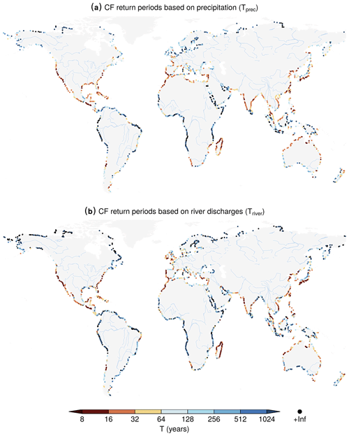
Figure 1 Present-day (1980–2014) potential compound-flooding probability based on precipitation and on river discharge. Return periods of CF defined as co-occurring extremes (5-year return levels) of the CF drivers. Return period of co-occurring (a) storm surge (including waves) and precipitation (accumulated 3 d centred) extremes and (b) storm surge (including waves) and river discharge extremes. Major rivers are shown in light blue. Infinite values are shown in black.

We qualitatively investigate how the two assessments compare for different classes of catchment size. To do so, we rank the rivers based on their catchment size and divide them into groups having the same sample size; for each group we compute different statistics to compare the two assessments: the Spearman correlation of T_river and T_prec, the ratio of T_river∕T_prec, and the percentage of locations with T_river compatible to T_prec. This binning procedure provides equally robust statistics for each bin and shows similar results for small variations in the bin size.

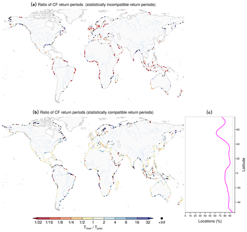
Figure 2 Difference between the present-day (1980–2014) potential compound-flooding probability based on precipitation and on river discharge. Ratio (T_river∕T_prec) of CF return period of concurring river discharge and storm surge extremes (T_river) to CF return period of concurring precipitation (accumulated 3 d centred) and storm surge extremes (T_prec). (a) The ratio where T_river is statistically incompatible (at 95 % confidence level; see Methods) with T_prec. (b) The ratio where T_river is statistically compatible with T_prec, while (c) shows the coastline fraction where this happens (binned every 5^∘ of latitude and smoothed using a spline function). In (c), the dashed grey line shows the 95 % level.

2.1.1 Results and discussion

The spatial patterns of the potential CF return periods based on either precipitation (T_prec) or river discharge (T_river) are very similar (Fig. 1; Fig. A2 is identical but shows results based on extremes defined considering 2-year return levels). The results for clusters of locations with the 5 % lowest CF return periods are also similar in the two assessments (Figs. A3 and A4). These hotspot regions are mainly found along the US, Central American, and southern North Atlantic coasts and in central Chile, Madagascar, and southern Japan.

While the spatial patterns of the CF return periods obtained from the two approaches are very similar, their relative differences can be substantial, especially at certain locations (Figs. 2 and A5). Given that the return period computation procedure involves several uncertainty factors (e.g. bivariate model fitting and the definition of the return levels), we test the hypothesis that the return period based on the river discharge is statistically compatible (at a 95 % confidence level) with that based on precipitation. When defining extremes based on the 5-year return levels, the river-based return period is compatible with the precipitation-based value in about 82 % of the locations (Fig. 2c; 76 % for 2-year return levels; Fig. A5c). The spatial distribution of locations where T_river is not statistically compatible with T_prec does not seem to follow a clear spatial pattern, though it appears that T_river is lower than T_prec in northern Europe and in the tropics. The latter are areas where CF is unlikely. T_river is higher than T_prec along the Gulf of Mexico (Figs. 2c and A5c). Compatible T_river and T_prec values are found but with large discrepancies in the tropics and above 60^∘ N (Fig. 2b), consistent with the high uncertainty of these large CF return periods that do not allow for detecting potential differences between T_river and T_prec.

In areas with a tendency towards high CF return periods, e.g. the tropics, neighbour locations show divergent values in the ratio between the return periods of the two assessments (dark-blue and red dots in Fig. 2). Further tests showed that this behaviour is not related to the goodness of fit of the bivariate distributions; rather it appears associated with the large uncertainties of high return periods and potentially with different catchment characteristics.

We find that there is a tendency towards higher differences in the two assessments at locations where either or both T_prec and T_river are high (i.e. where T approaches the value expected under the independence of the CF drivers; Fig. A6). (This appears consistent with the high uncertainty associated with large CF return periods.) Such a finding has relevant implications, as it indicates that the two assessments tend to be similar, on average, where assessing the actual CF is more important, i.e. where there is a relatively high CF potential (Fig. A6).

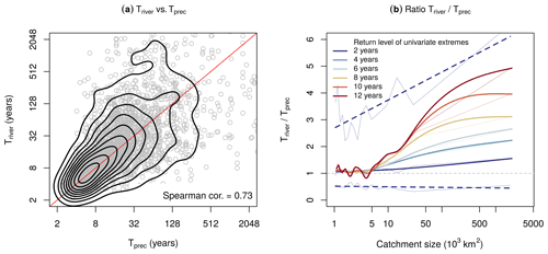
The spatial association of the return period map obtained from the two assessments is shown in Figs. 3a and A7a. The Spearman correlation between T_river and T_prec is ∼0.7 and increases as the return level threshold employed to define the extremes decreases, e.g. 0.66 and 0.73 for the 5- and 2-year return level, respectively (Figs. 3a and A7a). This trend in the correlation is consistent with the higher uncertainties characterising larger return periods.

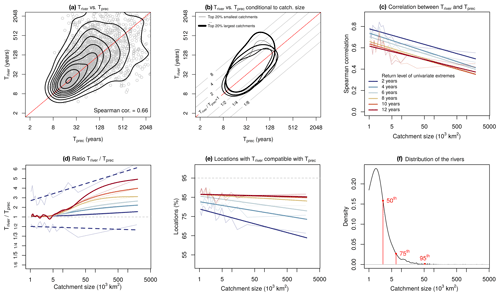
Figure 3 Comparison of the potential compound-flooding probability based on precipitation and on river discharge. (a) Scatterplot (based on Fig. A2) of CF return periods based on river discharge (T_river) and on precipitation (T_prec) for extremes defined based on 5-year return levels. Black contours represent the isolines of the kernel density containing from 10 % to 90 % of the (T_river, T_prec) pairs. The identity line is shown in red. (b) Empirical probability density function of the variables (T_river, T_prec) conditioned on the catchment size; the thickness of the isolines increases with the catchment size such that each bin considers one fifth of the total number of analysed rivers (3178). Each contour line (isolines of the kernel density) contains about 50 % of the (T_river, T_prec) pairs. (c-e) Statistics comparing T_river and T_prec as a function of the catchment size and of the return levels used to define the CF univariate extremes (see legend in a). (c) Spearman correlation between the maps of T_river and T_prec. (d) T_river∕T_prec ratio. The dashed line is the centred 68 % (16th–84th percentiles) confidence interval of the ratio based on the 2-year return levels. A non-linear y axis for values below 1 is plotted such that the specular cases, e.g. ratio r=2 ($T_{\mathrm{river}}=\mathrm{2}\cdot T_{\mathrm{prec}}$) and $r=\mathrm{1}/\mathrm{2}$ ($T_{\mathrm{prec}}=\mathrm{2}\cdot T_{\mathrm{river}}$) (see b), appear symmetric with respect to r=1 (T_river=T_prec). (To obtain the plot, the ratio is defined as $r=T_{\mathrm{river}}/T_{\mathrm{prec}}$; then if r<1, r is transformed to $r=-T_{\mathrm{prec}}/T_{\mathrm{river}}+\mathrm{2}$. Now e.g. r=2 and r=0 represent specular cases; therefore, where the y axis is r=0, 1, 2, …, we can write $r=\mathrm{1}/\mathrm{2}$, 1∕3, 1∕4, ….) See Fig. A7b for the plot with a standard axis. (e) Percentage of locations where T_river is statistically compatible with T_prec at the 95% confidence level. (f) Probability density function of the catchment size of the analysed rivers; 50th, 75th, and 95th percentiles of the distribution are shown in red. In (c–e), thick lines are obtained through regressing the obtained statistical values per bin (thin lines) to the natural logarithm of the mean size of the catchment bins. All lines are regressed using linear regression, except from the median of the ratio in (d), where a spline function is used. The slopes of the linear regressions are all significant in (c) (p value < 0.0024) and significant up to the 6-year return level in (e) (p value < 0.022).

Although some of the differences between the two assessments can be driven by uncertainties in the return period estimation, also several physical processes, e.g. topography-dependent ones, may be involved. The Spearman correlation between the two assessments decreases (p value < 0.0024) as the catchment size increases (Fig. 3c). The latter suggests that – for larger catchments – different processes may cause either positive or negative deviations between T_river and T_prec.

Water levels in the mouth of small rivers are expected to be largely influenced by the precipitation around the coast (Hendry et al., 2019; van den Hurk et al., 2015; Bevacqua et al., 2017), while around large rivers, inland hydrological processes are usually dominant. Therefore, we qualitatively investigate whether the actual difference between the two assessments (quantified as T_river∕T_prec) depends on the size of the catchment (Hendry et al., 2019). For example, the T_river∕T_prec ratio, defined using the 5-year return level, tends to increase with the catchment size (Fig. 3b; see the deviation of the scatterplot of T_river vs. T_prec from the identity line emerging with the increasing dimension of the catchment). For CF return periods defined based on 2-year return level extremes, the median T_river∕T_prec ratio is near unity for most of the catchments, even though the T_river∕T_prec ratio increases slightly for larger catchments (blue line in Fig. 3d). For higher return levels, the median T_river∕T_prec ratio increases with the size of the catchment (Fig. 3d), indicating that the CF assessments based on precipitation and river discharge differ largely for large rivers. For all return levels, the median T_river∕T_prec ratio is near unity for rivers whose catchment size is up to about 5–10×10³ km² (Fig. 3d), i.e. about 75 % of the rivers presently analysed (Fig. 3f). Binning the rivers per catchment size, we find that the variance of the T_river∕T_prec ratio within each bin tends to be smaller for small rivers than for large rivers (Fig. 3d, shown by the dashed line for the 2-year return level). However, it is important to highlight that there is substantial variance (Fig. 3d for the 2-year return level extremes), and that for a river of any catchment size the associated T_river∕T_prec ratio can be either small or large. Overall, the similarity of T_river and T_prec for small rivers is highlighted by the fact that for small rivers it is more likely that T_river is statistically compatible with T_prec (Fig. 3e). For example, Fig. 3e (4-year return level curve) shows that T_river is statistically compatible with T_prec for ∼82 % of the small rivers (catchment size < 5000 km²) and for ∼75 % of large rivers (catchment size > 50 000 km²). The decrease in the compatibility of T_river and T_prec with the catchment size (Fig. 3e) is statistically significant for return levels smaller than the 6-year return level (p value < 0.022). However, for high return levels this decrease is not prominent, most likely due to the large uncertainty associated with longer return periods. Figure 3e indicates the discrepancy for large catchments in the T_river∕T_prec ratio being greater for low return levels, whereas Fig. 3d indicates the opposite; this is also likely caused by the larger uncertainty of return periods of higher return levels, which does not allow for detecting potential differences between large values of T_river and T_prec.

The differences between T_river and T_prec are not only controlled by the catchment size but can be the result of several other factors. During the hydrological modelling, input data artefacts or model inaccuracies, among other factors, introduce uncertainty which may contribute to the observed differences. Another important contribution should arise from the uncertainties in the bivariate return period estimation (Bevacqua et al., 2019; Wahl et al., 2015), which can contribute to both positive and negative deviations between T_river and T_prec. Moreover, the catchment response time to precipitation depends also on rock and soil catchment permeability (Hendry et al., 2019). Finally, river discharge is influenced not only by local coastal precipitation but also by the weather over the previous weeks or months over the catchment, including evaporation and potentially snowmelt (Couasnon et al., 2020; Bevacqua et al., 2017).

Clearly, the diversity of the physical processes leading to CF_prec and CF_river is very relevant and can cause both positive and negative differences between T_river and T_prec (Blöschl et al., 2019). For example, for any given catchment, a slow catchment response time may either increase or decrease the T_river∕T_prec ratio. In locations where cyclones cause frequent concurring storm surge and widespread coastal precipitation, it is not guaranteed that CF_river probability will be also high. For example, if the rainfall in the catchment upstream needs time to reach the coast long enough for the storm surge to recede, then CF_river will be unlikely, and in this case the T_river∕T_prec ratio will be high (Klerk et al., 2015; Ward et al., 2018). In contrast, where the CF_prec is unlikely because different weather systems cause precipitation and storm surge extremes, a relatively slow catchment response time may sometimes allow for high river discharge and storm surge to concur if e.g. a first cyclone causes precipitation driving high river discharge reaching the coast when a second cyclone drives a storm surge (contributing to a low T_river∕T_prec ratio; Bevacqua et al., 2019).

In addition the presence of a pronounced annual cycle in river discharge can modulate the river-discharge-driven CF hazard and thus the T_river∕T_prec ratio. In regions where CF_prec is likely, CF_river may be unlikely if the storm surge season does not coincide with the season of the high river discharge (high T_river∕T_prec ratio;  Ward et al., 2018). In contrast, where the CF_prec is unlikely, CF_river may be more likely if the storm surge season coincides with the high-river-discharge season (low T_river∕T_prec ratio). In addition, precipitation extremes are typically short in duration, while river discharge extremes are less dynamic. Although events exceeding the α-year return level threshold occur both for precipitation and river discharge on average every α years, the number of days with high river discharge can be larger than the number of days with a high precipitation amount. From a statistical point of view, the above mechanism alone would make CF_river more likely than CF_prec (low T_river∕T_prec ratio; this effect is even more pronounced in catchments with a slow response time and especially in areas where different weather systems cause precipitation and storm surge extremes; Bevacqua et al., 2020). The above effect is weakened as the return level threshold used to define extremes increases due to the shorter duration of river discharge extremes. The above considerations justify the T_river∕T_prec ratio increasing with the return level choice (Fig. 3d).

While the relevance of the mechanisms discussed above may depend on the local climate, they are expected to be less relevant in very small rivers where the catchment response time is small, and thus autocorrelation in the river time series is smaller. Consistently, we find that T_river and T_prec tend to match more in smaller catchments. However, a higher agreement for small rivers might also arise from the relatively coarse spatial resolution of the data which would attenuate differences between precipitation and river discharges in small rivers. Overall, we find that independent of the catchment size, T_river tends to be higher than T_prec on average (Fig. 3d), suggesting that the mechanisms causing T_river>T_prec may be more likely or relevant. Apparently this is a general remark and not a universal law, since there are also several locations where T_prec exceeds T_river.

The presented results are based on state-of-the-art model data which have been validated and discussed in previous papers (Vousdoukas et al., 2018; Beck et al., 2017a; Couasnon et al., 2020; Bevacqua et al., 2019; Muis et al., 2016). However, the above-mentioned validation efforts did not include areas where field measurements are scarce, like parts of South America, Africa, and Asia (Ward et al., 2018). At high latitudes, ice and snow dynamics apply a certain control to both river hydrology (Yamazaki et al., 2014) and wave and storm surge dynamics (Vousdoukas et al., 2017). However, such processes are not resolved by the global models used to generate the forcing datasets used in the present study. For these reasons, the present findings should be interpreted with care, especially in northern regions (Couasnon et al., 2020).

The two approaches investigated here provide information only on the potential for CF. The actual CF occurrence depends also on the local topography which can favour or not favour the interaction between the CF drivers; also, concurrent but not hydrologically interacting storm surges and pluvial or fluvial flooding are relevant as they can e.g. limit the ability to respond to emergency and amplify the impacts that the two hazards would have caused if they occurred in isolation (Martius et al., 2016; Barton et al., 2016; Zscheischler et al., 2019). Moreover, while the two approaches investigated here are supposed to represent different CF mechanisms, separating the CF mechanisms in this way could be misleading, as CF may happen due to a combination of river discharge, local rainfall and associated surface runoff, and high sea level. For example, in July 2019, New Orleans (Louisiana, USA; Vahedifard et al., 2016) was simultaneously threatened by Hurricane Barry causing local rainfall and a storm surge around the coast and by extremely high water discharge from the Mississippi River which lasted from March to July. CF risk assessment at the local scale should be carried out via complex hydrological modelling that can take into account the complex mechanisms causing CF, including storm surges, waves, astronomical tides, and when necessary not only fluvial or pluvial flooding but also their combination.

3 Conclusions

We conduct two global-scale potential CF hazard assessments, using either storm surge and precipitation or storm surge and river discharge model data, and we then compare how the choice of precipitation vs. river discharge as a covariate with storm surge affects the results. We find that the two approaches result in similar spatial CF hazard patterns, which tend to deviate as the river catchment size increases. In addition, on average, the deviations between the two assessments are smaller in regions where assessing the actual CF is more relevant, i.e. where the CF potential is high.

Due to data scarcity, current large-scale CF assessments rely on approaches and model-based datasets similar to those used here. This study indicates that for these large-scale assessments, a precipitation-based CF analysis can provide satisfactory information on the CF potential in estuaries of small- and medium-sized rivers (catchment smaller than about 5–10×10³ km²). Moreover, a precipitation-based CF analysis allows for assessing the CF hazard arising from the interaction of local coastal rainfall and storm surges where no rivers exist or along the mouths of small rivers often not represented in global river datasets. Naturally, employing river discharge data should always be preferred to using precipitation when studying both the large- and local-scale CF in estuaries, when data are available, especially in areas where we detected large differences between the two approaches. The importance of using river discharge data is even greater in estuaries of long rivers.

Appendix A: Supporting figures

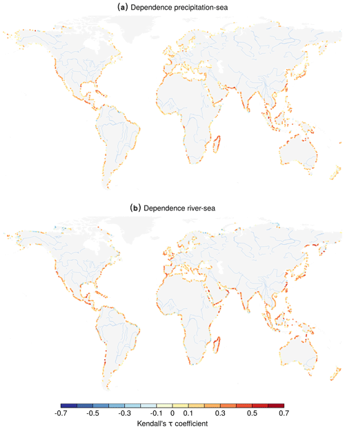
Figure A1 Kendall's τ correlation associated with the copulas fitted to the selected pairs of (a) precipitation and sea level and (b) river discharge and sea level.

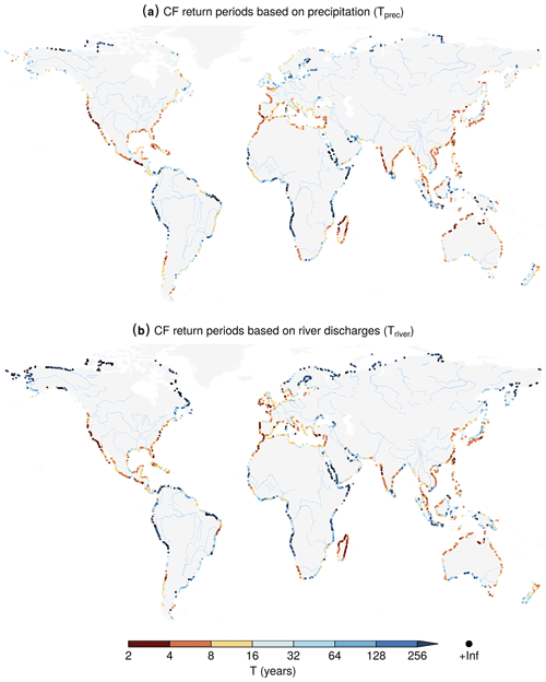
Figure A2 The same as Fig. 1, but the extremes are defined as 2-year return levels.

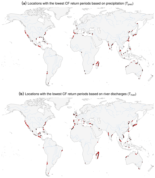
Figure A3 Locations with the lowest potential compound-flooding probability based on precipitation and on river discharge. Locations with return periods below the 10th and 5th percentile are shown in black and red, respectively. The extremes are defined considering 5-year return levels. CF return periods are based on precipitation in (a) and on river discharge in (b).

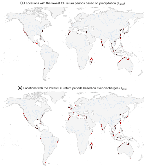
Figure A4 The same as Fig. A3, but the results are based on extremes defined considering 2-year return levels.

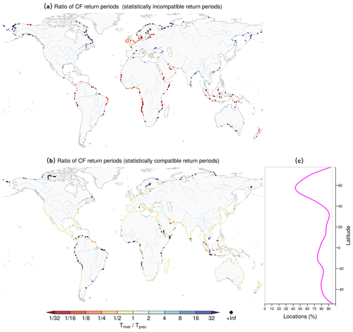
Figure A5 The same as Fig. 2, but the results are based on extremes defined considering 2-year return levels.

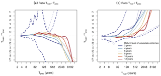
Figure A6 (a) Ratio between the CF return periods based on river discharge (T_river) and on precipitation (T_prec) as a function of T_prec (and of the return levels used to define the CF univariate extremes; see legend in b). The dashed line is the centred 68 % (16th–84th percentiles) confidence interval of the ratio based on the 2-year return levels. Thick lines are obtained through regressing the investigated statistical values to the natural logarithm of the mean return period of the bins via a spline function. (b) The same as (a), but the ratio is conditioned on T_river. As in Fig. 3d of the original paper, a non-linear y axis for values below 1 is employed such that the specular cases, e.g. ratio r=2 ($T_{\mathrm{river}}=\mathrm{2}\cdot T_{\mathrm{prec}}$) and $r=\mathrm{1}/\mathrm{2}$ ($T_{\mathrm{prec}}=\mathrm{2}\cdot T_{\mathrm{river}}$) (see Fig. 3b), appear symmetric with respect to r=1 (T_river=T_prec).

Figure A7 (a) The same as Fig. 3a, but the results are based on extremes defined considering 2-year return levels (the figure is based on Fig. A2). (b) As Fig. 3d but with a linear y axis.