Estimation of tropical cyclone wind hazards in coastal regions of China

Coastal regions of China feature high population densities as well as wind-sensitive structures and are therefore vulnerable to tropical cyclones (TCs) with approximately six to eight landfalls annually. This study predicts TC wind hazard curves in terms of design wind speed versus return periods for major coastal cities of China to facilitate TC-wind-resistant design and disaster mitigation as well as insurance-related risk assessment. The 10 min wind information provided by the Japan Meteorological Agency (JMA) from 1977 to 2015 is employed to rebuild TC wind field parameters (radius of maximum winds R_max,s and shape parameter of radial pressure profile B_s) at surface level using a height-resolving boundary layer model. These parameters will be documented to develop an improved JMA dataset. The probabilistic behaviors of historical tracks and wind field parameters at the first time step within a 500 km radius subregion centered at a site of interest are examined to determine preferable probability distribution models before stochastically generating correlated genesis parameters utilizing the Cholesky decomposition method. Recursive models are applied for translation speed, R_max,s and B_s during the TC track and wind field simulations. Site-specific TC wind hazards are studied using 10 000-year Monte Carlo simulations and compared with code suggestions as well as other studies. The resulting estimated wind speeds for northern cities (Ningbo and Wenzhou) under a TC climate are higher than code recommendations, while those for southern cities (Zhanjiang and Haikou) are lower. Other cities show a satisfactory agreement with code provisions at the height of 10 m. Some potential reasons for these findings are discussed to emphasize the importance of independently developing hazard curves of TC winds.

1 Introduction

Tropical cyclones (TCs) are rapidly rotating storms characterized by strong winds, heavy rain, high storm surges and even devastating tornadoes. They inflict tremendous damage on property and considerable loss of human life and pose threats to flexible structures in coastal areas (Done et al., 2020). In the western Pacific basin, TCs form throughout the year. It is the most active TC basin in the world, producing more than 30 storms annually, accounting for almost one-third of the global total (Knapp et al., 2010; Yang and Chen, 2019). The southeast China coastal area has long coastlines and numerous islands, which feature high population densities as well as many wind-sensitive structures including high-rise buildings and long-span bridges (Tao et al., 2018; Tao and Wang, 2019). It is a TC-prone region, with an average of six to eight TC landfalls per year. It has been estimated that more than 1600 fatalities and CNY 80 billion of direct economic loss can be attributed to TCs and subsequent floods in 2006 alone in coastal regions of China (Liu et al., 2009), demonstrating that this area is extremely vulnerable to TC damage. Accordingly, it is an issue of great importance to analyze TC wind hazards to support wind-resistant design as well as disaster mitigation and insurance-related risk assessment.

Unlike non-TC winds such as monsoons, TCs are moving rotating storms with a small occurrence rate at a specific location. Moreover, wind anemometers are usually vulnerable to damage during strong typhoon events, making the record of historically observed winds an unreliable predictor for design wind speed based on statistical distribution models. The largest yearly wind speed dataset derived from both non-TC and TC winds is considered to be not well behaved because the contribution of each wind speed to describe the probabilistic behavior of the extreme winds is inhomogeneous (Simiu and Scanlan, 1996). An alternative approach, called stochastic simulation or Monte Carlo simulation, introduced in the 1970s by some pioneering studies (e.g., Russell and Schueller, 1974; Batts et al., 1980), has been widely adopted to stochastically generate a large number of wind speed samples using historical data-based probability distributions of several key field parameters. In order to achieve TC hazard assessment by Monte Carlo simulation, the circular subregion method (CSM) was developed by Georgiou (1985) and later employed by Vickery and Twisdale (1995), Xiao et al. (2011), and Li and Hong (2015). The CSM uses the circled historical track information centered on the site of interest to characterize the statistics of some TC parameters before conducting storm simulation and wind speed prediction. This is a site-specific approach. The state-of-the-art empirical full-track technique was first developed by Vickery et al. (2000b) and followed by FEMA (Federal Emergency Management Agency, 2015) as well as the ASCE 7-16 loads standard (ASCE STANDARD, 2017) and Li and Hong (2016), which simulates the TC tracks as well as the intensity in terms of a relative intensity index from genesis to lysis, facilitating the TC risk assessments for the whole coastal region. Although the full-track model is preferable for modeling the TC hazards along the whole coastline, the CSM is widely used for some site-specific TC risk studies and can be easily updated and improved by supplementary observations. This is also adopted in this study.

During TC wind estimation, the parametric TC wind field model has been commonly adopted and has been continuously improved over the past several decades based on the ever increasing number of observation data. This model is considered to be more economical with time and even more accurate in predicting TC wind velocity compared with some meteorological models. Some pioneering studies on parametric TC wind field modeling have been performed since the 1980s (Batts et al., 1980; Georgiou, 1985; Vickery et al., 2000a, 2009; Nederhoff et al., 2019; Arthur, 2019). These studies employed a gradient wind speed model solved by the atmospheric balance equation of a stationary storm coupled with a depth-averaged (Vickery et al., 2000a) or a semiempirical observation-based boundary layer vertical profile model (Vickery et al., 2009). In recent years, with advances in computing capacity, another more sophisticated physical model has received intensive attention. This is the so-called height-resolving model, in which the boundary layer wind field is solved semianalytically based on 3D Navier–Stokes equations (Meng et al., 1995; Kepert, 2010; Snaiki and Wu, 2017; Fang et al., 2018a). This is of great help in interpreting the underlying physics of the TC boundary layer.

Conventionally, wind field parameters such as the radius of maximum wind speed R_max and shape parameter of radial pressure profile B were statistically modeled as functions of surface central pressure deficit, TC eye center latitude and sea surface temperature (Vickery et al., 2000b; Vickery and Wadhera, 2008; Xiao et al., 2011; Zhao et al., 2013; FEMA, 2015; Fang et al., 2018b). This facilitated TC-related hazard assessment by carrying out a large number of scenarios using a Monte Carlo algorithm since the historical track information is readily available in each best-track dataset. However, the correlations between these parameters were not very strong, as shown by Vickery et al. (2000b), with all coefficients of determination less than 0.30. The auto correlations of R_max as well as B between different time steps in these studies were usually propagated from surface pressure deficit and sea surface temperature, which were integrated with a term of relative intensity and modeled by a recursive model. Moreover, the cross-adoption of these parameter models in different basins could cause some undesired results since they are always region dependent due to differences among macroscopic atmospheric thermodynamic environments.

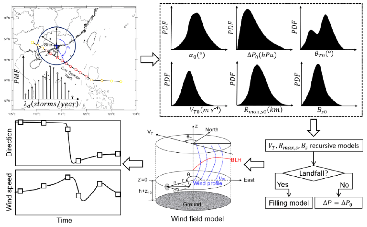
Figure 1 Overview of circular subregion method used in this study.

In this study, wind field information of a 10 min time duration provided by the best-track dataset of the Japan Meteorological Agency (JMA) was adopted to develop a dataset of R_max and B at surface level (R_max,s and B_s) using a height-resolving wind field model. Then the TC design wind speed was predicted by following the procedures illustrated in Fig. 1. Based on the historical track information extracted from the JMA dataset within a circular subregion with a radius of 500 km centered at the site of interest, the preferable probabilistic distributions of six genesis parameters at the first time step, the position of the first track dot (α₀), heading direction (θ_T0), central pressure difference (ΔP₀), translation speed (V_T0), R_max,s0 and B_s0 were determined before performing the correlation analyses. Site-specific recursive models of translation speed as well as of R_max,s0 and B_s0 were developed using the track information within the circular subregion. Finally, 10 000-year Monte Carlo simulations were conducted to investigate the TC wind hazard for 10 coastal cities of China.

2 Statistical characteristics of TC tracks

2.1 JMA best-track dataset

In the western Pacific basin (0–60^∘ N, 100–180^∘ E), the Japan Meteorological Agency (JMA) serves as the Regional Specialized Meteorological Center (RSMC Tokyo-Typhoon Center, 2018), as specified by the World Meteorological Organization (WMO). As such, it is responsible for forecasting, naming, tracking, distributing warnings of and issuing advisories on TCs. Accordingly, the JMA has been publicly releasing best-track datasets of TCs in the western Pacific basin since 1951. These datasets contain not only some basic track information of TCs in terms of latitude and longitude of TC eye centers as well as dates and times but also some wind speed information including minimum surface central pressure (P_cs), maximum sustained surface wind speed (V_max,s) and 50- or 30-knot (1 knot =0.514 m s⁻¹) wind radii estimated from surface observation, ASCAT observation and low-level cloud motion satellite images. Although some other organizations issue their own track dataset of TCs for the western Pacific basin (Ying et al., 2014), such as the China Meteorological Administration (CMA), Joint Typhoon Warning Center (JTWC), Hong Kong Observatory (HKO) and International Best Track Archive for Climate Stewardship (IBTrACS) project, there are some inconsistencies among these datasets that should be carefully considered. In addition to differences in TC track information and annual TC frequencies, two typical TC intensity representations, i.e. P_cs and V_max,s, show inconsistency from agency to agency, as discussed by Song et al. (2010). Generally, a remarkable difference was found, i.e., that $V_{\max ,\mathrm{s}}\left(\mathrm{JTWC}\right)>V_{\max ,\mathrm{s}}\left(\mathrm{CMA}\right)>V_{\max ,\mathrm{s}}\left(\mathrm{JMA}\right)$ and $P_{\mathrm{c}}\left(\mathrm{JTWC}\right)<P_{\mathrm{c}}\left(\mathrm{CMA}\right)<P_{\mathrm{c}}\left(\mathrm{JMA}\right)$ when TCs reach typhoon level, and this trend becomes apparent along with storm intensification (Song et al., 2010). It could be attributed to time interval differences since the JMA uses 10 min and the CMA uses 2 min, while the JTWC uses 1 min. The differences among estimation techniques and algorithms for determining V_max,s and P_cs based on the Dvorak technique (Dvorak, 1984; Velden et al., 2006) with satellite cloud images could also contribute to this inconsistency. However, the 10 min time duration employed by the JMA is consistent with most design codes or standards and is also suggested by the WMO (Fang et al., 2019a). Furthermore, the 50-knot or 30-knot radii information provided by the JMA dataset is a supplement of great importance in facilitating the estimation of TC wind field parameters. As a result, the JMA best-track dataset was selected as the basic information for the following TC hazards studies in the southeast China region.

2.2 Statistical correlations

In order to examine the statistical characteristics of historical track information around a site of interest, track segments that intersect and are within a circular subregion entered at the target location are usually extracted from the best-track dataset. The size of the subregion directly affects the data sampling as well as the final design wind speed prediction (Georgiou, 1985; Xiao et al., 2011; Li and Hong, 2015). A suitable circle size should enable the TC tracks and wind field parameters to be less sensitive and to cover as many high-wind-speed samples as possible. Three radii, 500, 1000 and 250 km, were employed by Vickery and Twisdale (1995), Xiao et al. (2011), and Li and Hong (2015), respectively. The use of 1000 km could overestimate the effects of high winds on a site of interest since some extremely violent typhoons over distant sea would be circled and used to model the central pressure before landfall. However, these typhoons have little chance of maintaining an extremely high intensity until landfall on mainland China. Based on the JMA dataset from 1951 to 2015, only seven violent typhoons (P_cs≤935 hPa or $V_{\max ,\mathrm{s}}\ge \mathrm{54}$ m s⁻¹, 105 knots), Nina (195307), Wanda (195606), Grace (195819), Saomai (200608), Hagupit (200814), Usagi (201319) and Rammasun (201409) directly landed on mainland China. Moreover, the largest R_max,s0, illustrated in Figs. 8 and 16, range from 500 to 600 km if the size of subregion R=500 km is employed. And as mentioned by Yuan et al. (2007), about 50 % of the radii of historical storms associated with a wind speed of 15.4 m s⁻¹ range from 222 to 463 km and only 10 % are larger than 555 km. In fact, we can show experimentally that at the outer regions of a typhoon, 500 km or more away from the storm center, there is only a slight influence on the specific region. Accordingly, R=500 km, which is consistent with Vickery and Twisdale (1995) and will be used in this study, allows as many high wind speeds as possible to be considered and avoids the overuse of some extremely violent typhoons.

Taking the example of the Hong Kong region (centered on 22.3186^∘ N, 114.1678^∘ E), which is severely affected by TCs, 412 segments of track data within a circle of R=500 km were captured from the JMA dataset (1951–2015), as shown in Fig. 2. Although few TCs originate in this circular region, they only reach the strongest level of a severe tropical storm, with P_cs larger than 980 hPa belonging to a normal-intensity storm. Their genesis locations are also close to the circular boundary. Accordingly, all simulated tracks can be assumed to originate from the circular boundary by considering the location distribution of historical tracks in terms of origin angle α₀, which is the direction relative to the site of interest and clockwise positive from the north.

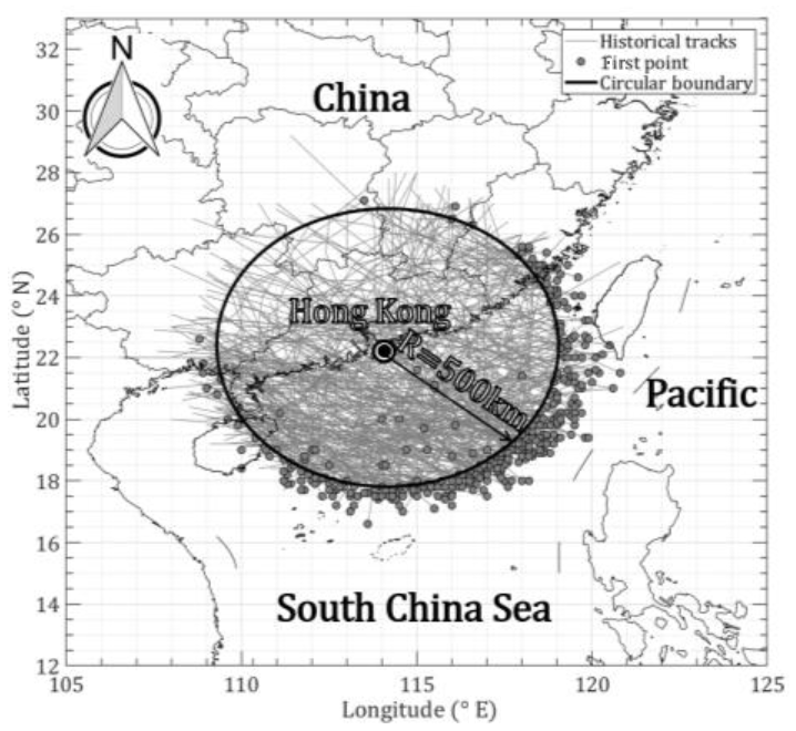
Figure 2 Track segments within a circular region centered on Hong Kong with a radius of 500 km.

Table 1 Distribution models and coefficients for TC track genesis parameters.

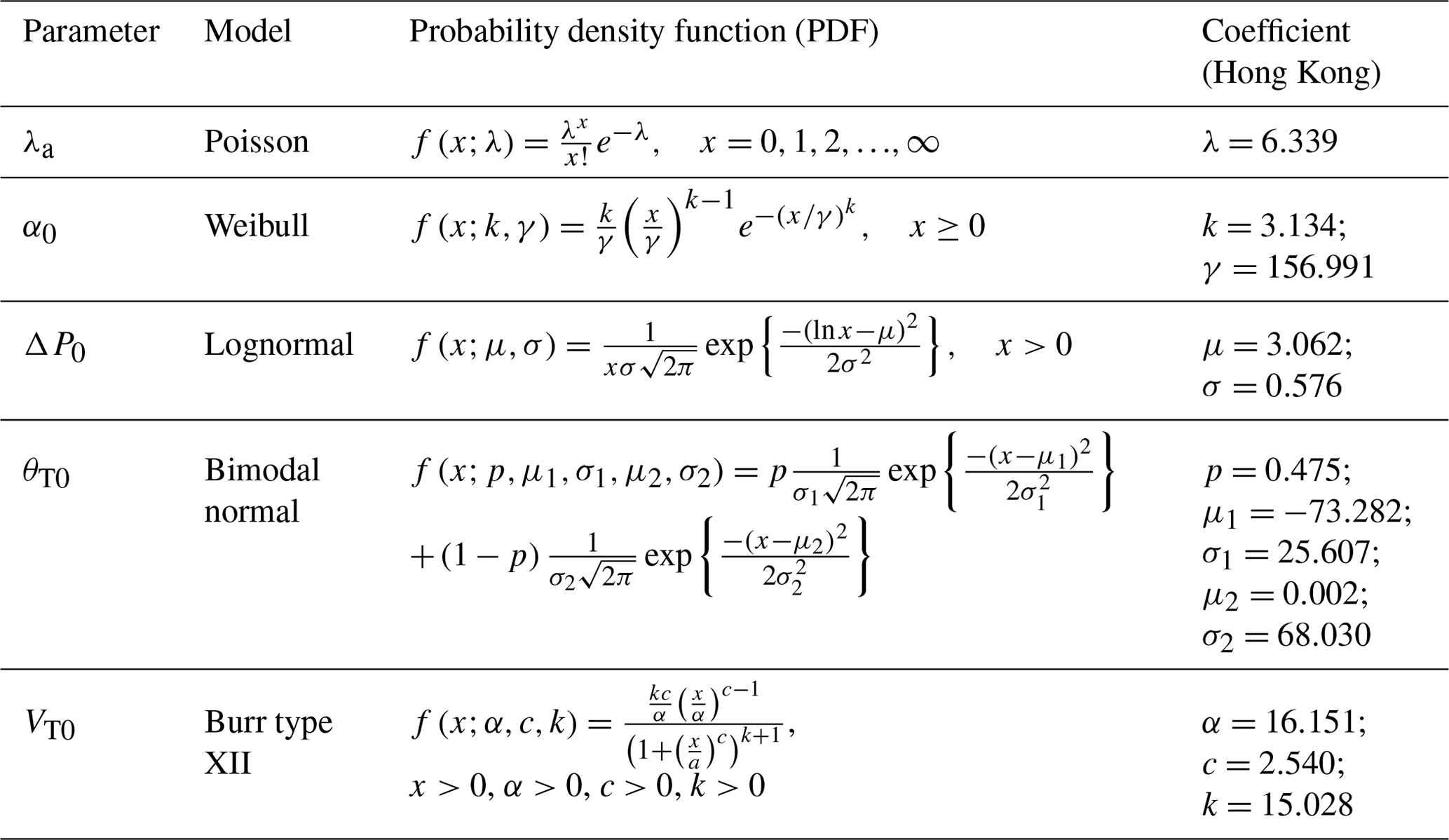
Note that x denotes the argument or the input of the function.

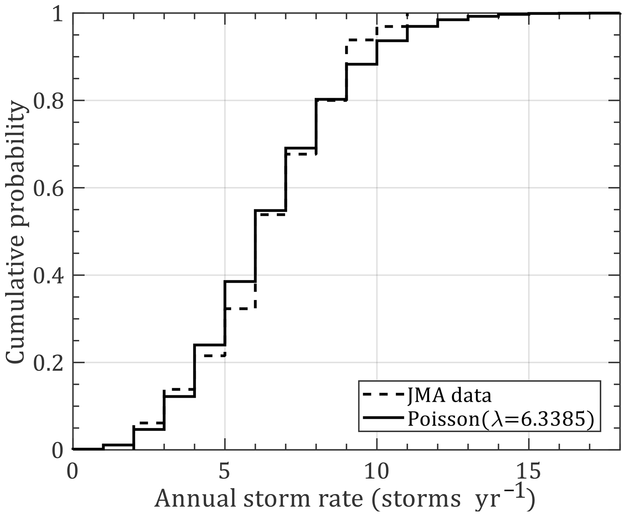
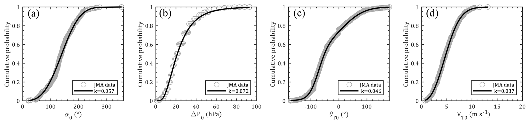
The annual storm rate (storms per year) is usually modeled by negative binomial (Li and Hong, 2016) or Poisson (Xiao et al., 2011; Li and Hong, 2015) distributions. However, the mean of the storm genesis within the circular region around Hong Kong is 6.339, which is larger than the variance of 2.280. It does not satisfy the prerequisite of the negative binomial distribution. The Poisson distribution was employed to model the annual storm rate (λ_a), as shown in Fig. 3. Based on the circular subregion method, the position of the first track dot (α₀) and its heading direction (θ_T0) determine the location of the simulated track line, while the translation speed (V_T0) is used to estimate the TC center location at each time step. First values of the central pressure difference (ΔP₀) for each segment are applied for the TC intensity modeling before landfall. Based on the statistical characteristics of historical data, the probabilistic distributions of these four parameters are fitted with several commonly used models using a maximum likelihood method before achieving the most suitable choices by the K–S (Kolmogorov–Smirnov) distribution test. The preferable distribution models, i.e., Weibull, lognormal, bimodal normal and Burr type XII, for all genesis parameters and their probability density functions (PDFs) together with fitted coefficients are listed in Table 1. Correspondingly, Fig. 4 compares the observed and modeled cumulative distribution functions (CDFs) for these parameters. The critical value of the K–S test for the historical data sample (n=204) is 0.0952 at a 5 % significance level larger than all the modeled results (values of k in Fig. 4), which proves that we have enough evidence to simulate the virtual TC tracks by adopting these distribution models. It noteworthy that all observed ΔP and θ_T values within the circle of interest are employed to model the distribution of ΔP₀ and θ_T0 due to the inherent drawback of the circular subregion method, which assumes for simplicity in the simulation that ΔP remains unchanged before the storm's landfall and θ_T is a constant for each TC track. All information of ΔP and θ_T can be taken into account to some extent when it is applied for modeling the distribution of ΔP₀ and θ_T0.

Figure 3 CDF of annual storm rate.

Figure 4 CDFs of track genesis parameters: (a) α₀; (b) ΔP₀; (c) θ_T0; (d) V_T0.

2.3 Translation speed

The translation speed is used for determining the TC eye locations at every time step and contributes slightly to the TC wind speed field. Traditionally, it was randomly sampled from a historical data-based probability distribution (Xiao et al., 2011; Li and Hong, 2015). In reality, the translation speed of the next step should be correlated with previous steps, which is also the statistical basis for empirical full-track modeling (Vickery et al., 2000b; Li and Hong, 2016). As the real data (historical observations) illustrate in Fig. 6a–c, the TC translation speed in the Hong Kong region is strongly dependent on the previous two steps with correlation coefficients of 0.7729 and 0.6281, while a weak correlation is observed with the heading angles. Accordingly, given the initial storm forward speed, the new speed for next steps can be modeled as a recursive formula

$$\begin{array}{}\text{(1)}& \begin{array}{rl}\ln V_{\mathrm{T}}\left(i+\mathrm{1}\right)& =v_{\mathrm{1}}+v_{\mathrm{2}}\cdot \ln V_{\mathrm{T}}\left(i\right)+v_{\mathrm{3}}\cdot \ln V_{\mathrm{T}}\left(i-\mathrm{1}\right)\\ & +v_{\mathrm{4}}\cdot {\mathit{\theta }}_{\mathrm{T}}\left(i+\mathrm{1}\right)+{\mathit{\epsilon }}_{\ln V_{\mathrm{T}}},\end{array}\end{array}$$

in which v_j (j=1–4) are model coefficients obtained from the least-squares regression analysis for historical data, V_T(i) is the translation speed at time step i, and ${\mathit{\epsilon }}_{\ln V_{\mathrm{T}}}$ is the error term accounting for modeling differences between the regression models and the real observations.

Figure 5 Logarithmic modeling errors for translation speed: (a) scatterplot; (b) CDF.

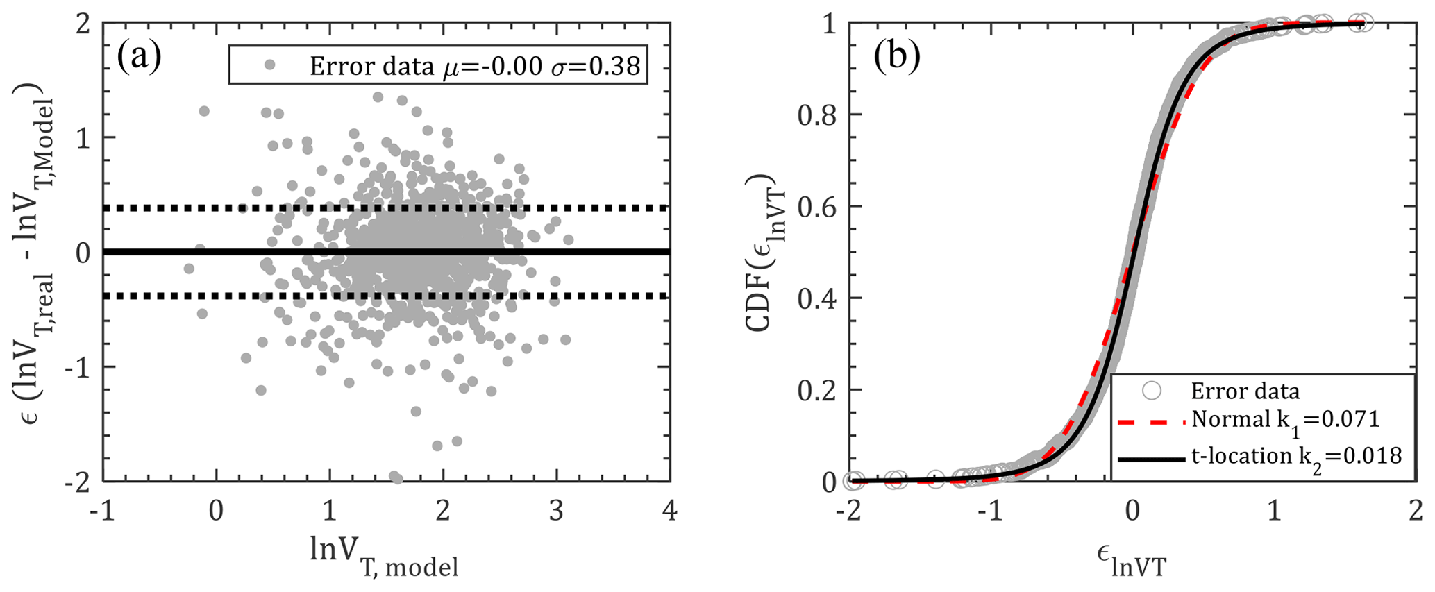
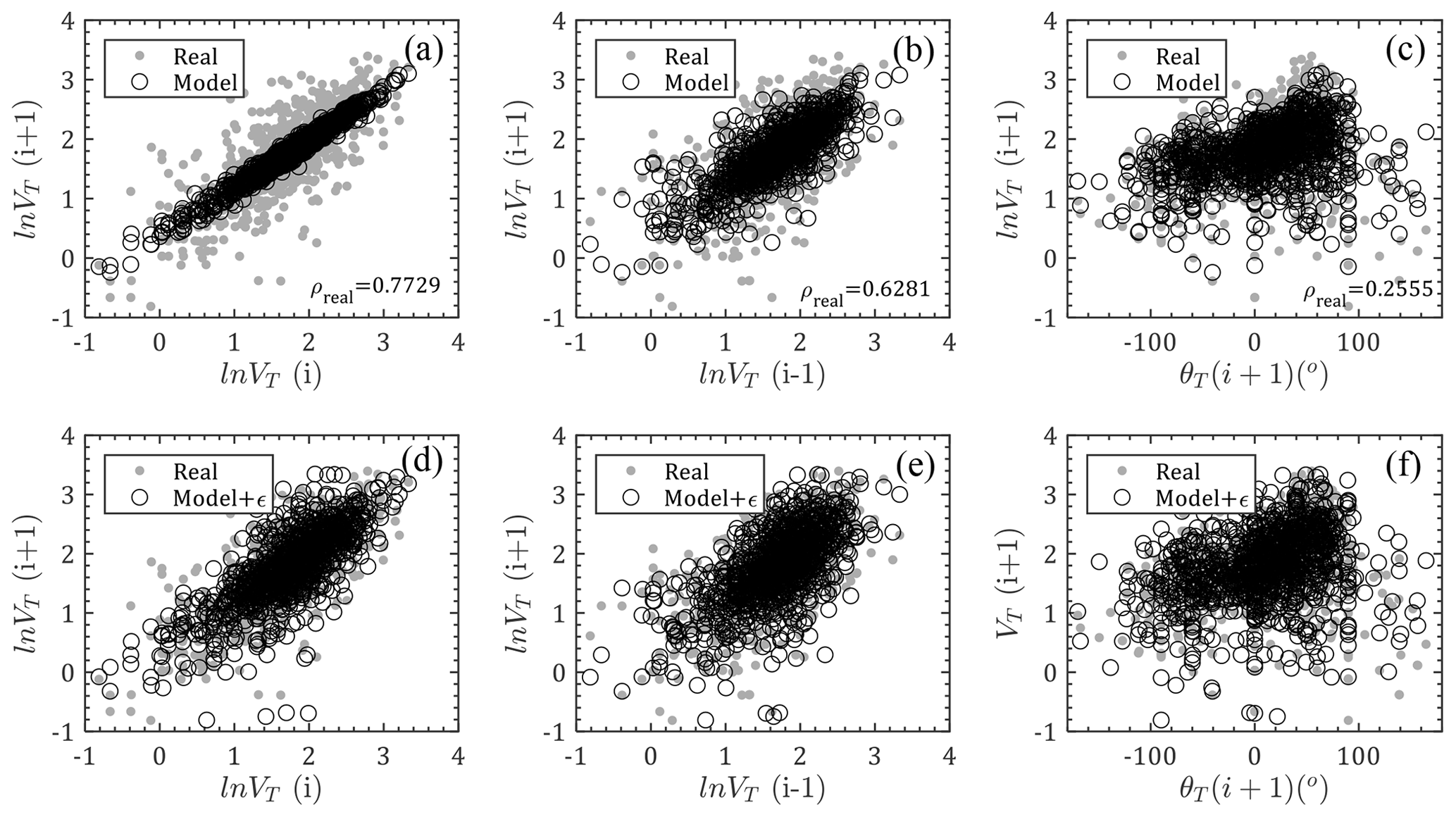
Figure 6 Comparison of translation speed between model and real observations: (a–c) relations between ln V_T(i), ln V_T(i−1), θ(i+1) and ln V_T(i+1) without errors; (d–f) relations between ln V_T(i), ln V_T(i−1), θ(i+1) and ln V_T(i+1) with errors; (ρ_real is the correlation coefficient for real observation data).

Based on the JMA dataset, the values of v_j (j=1–4) are extracted as 0.3089, 0.6338, 0.1504 and 0.0001 for the circular Hong Kong region. Model errors, as illustrated in Fig. 5a, are randomly distributed with a mean and standard deviation of 0 and 0.38, respectively, which indicates that the model is unbiased and has no obvious trend. These errors are then statistically fitted with two types of probability distribution models, i.e., normal distribution and t location-scale distribution, which are formulated by the PDFs as

$$\begin{array}{}\text{(2)}& {\displaystyle }f\left(x;\mathit{\mu },\mathit{\sigma }\right)={\displaystyle \frac{\mathrm{1}}{\mathit{\sigma }\sqrt{\mathrm{2}\mathit{\pi }}}}\exp \left\{{\displaystyle \frac{-{\left(x-\mathit{\mu }\right)}^{\mathrm{2}}}{\mathrm{2}{\mathit{\sigma }}^{\mathrm{2}}}}\right\},\text{(3)}& {\displaystyle }f\left(x;\mathit{\mu },\mathit{\sigma },\mathit{\nu }\right)={\displaystyle \frac{\mathrm{\Gamma }\left(\frac{\mathit{\nu }+\mathrm{1}}{\mathrm{2}}\right)}{\mathit{\sigma }\sqrt{\mathit{\nu }\mathit{\pi }}\mathrm{\Gamma }\left(\frac{\mathit{\nu }}{\mathrm{2}}\right)}}{\left[{\displaystyle \frac{\mathit{\nu }+{\left(\frac{x-\mathit{\mu }}{\mathit{\sigma }}\right)}^{\mathrm{2}}}{\mathit{\nu }}}\right]}^{-\frac{\mathit{\nu }+\mathrm{1}}{\mathrm{2}}},\end{array}$$

in which μσ and ν are location, scale and shape parameters. Γ(⋅) is the gamma function. As shown in Fig. 5b, the normal and t location-scale distributions are separately applied to fit the model errors using the maximum likelihood method. Although the fitting results for both distributions look good, the critical value of the K–S test for the observation data sample (n=1060) is 0.0418 at the 5 % significance level, which is smaller than the K–S value fitted by normal distribution (μ=0, σ=0.38) but larger than that fitted by t location-scale distribution (μ=0.0105, σ=0.2686, ν=3.5871). Consequently, t location-scale distribution is the preferable distribution for this case and will be used for error sampling.

As shown in Fig. 6, the forward speeds for next steps are modeled by Eq. (1) by introducing the historical track information and compared with observations. The first row (Fig. 6a–c) only considers the mean terms of Eq. (1), which indicates that the forward speed significantly depends on the previous steps using the linearly concentrated modeled mean values. The modeled mean values are more scattered with variation in translation speeds than with the previous second step and heading directions, but they are still within the scatter range of historical data. The second row, i.e., Fig. 6d–f, introduces the error term (${\mathit{\epsilon }}_{\ln V_{\mathrm{T}}}$) modeled by t location-scale distribution (Eq. 3) as mentioned before, which shows good agreement with the JMA observations. That is, the translation wind speeds can be well generated using the recursive model of Eq. (1).

3 Wind field model

3.1 TC wind field solutions

A height-resolving TC boundary layer model developed by Meng et al. (1995) and enhanced by Fang et al. (2018a) is adopted in this study. It is also used to extract two typical TC wind field parameters: radius of maximum wind speed (R_max,s) and radial pressure profile shape parameter (B_s) at surface level. It is then used to estimate the TC wind speed. Like most parametric TC wind field models, the surface pressure distribution in the radial direction is always prescribed and formulated by the Holland (1980) model, which is empirically determined by the location parameter (R_max,s) and the shape parameter (B_s) to solve the air pressure term in the Navier–Stokes equation. By extending the Holland pressure model in the vertical direction using the gas state equation, accounting for the effects of temperature and moisture, a height-resolving parametric TC pressure field model (Fang et al., 2018a) is developed as

$$\begin{array}{}\text{(4)}& \begin{array}{rl}{P}_{rz}& =\left\{P_{\mathrm{cs}}+\mathrm{\Delta }{P}_{\mathrm{s}}\cdot \exp \left[-{\left({\displaystyle \frac{R_{\max ,\mathrm{s}}}{r}}\right)}^{B_{\mathrm{s}}}\right]\right\}\\ & \cdot {\left(\mathrm{1}-{\displaystyle \frac{gkz}{R_{\mathrm{d}}{\mathit{\theta }}_{\mathrm{v}}}}\right)}^{\frac{\mathrm{1}}{k}},\end{array}\end{array}$$

in which subscripts r, z and s denote values at radius r, height z and surface (nominal height 10 m), respectively. P_rz= air pressure at height z and radius r from the TC's axis (hPa); P_cs= surface central pressure (hPa); $\mathrm{\Delta }{P}_{\mathrm{s}}=P_{\mathrm{ns}}-P_{\mathrm{cs}}$ is the central pressure difference (hPa), where P_ns is the peripheral pressure (usually taken as the pressure associated with the outermost closed isobar, 1013 hPa in this study); g=9.8 N kg⁻¹ is gravitational acceleration; R_d=287 J (kg K)⁻¹ is the specific gas constant of dry air; θ_v= virtual potential temperature (K), and $k=R/c_p$ is the ratio of the gas constant of moist air (R) to specific heat at constant pressure (c_p). After that, the wind speed in free atmospheric air can be readily solved. The wind field solutions in the TC boundary layer based on the linearization of Navier–Stokes equations can be expressed as the sum of gradient wind speed (V_g) and decay wind speeds (u_dv_d) due to frictional effects. More details regarding the wind field solutions are available in Fang et al. (2018a), which are omitted herein for brevity. One improvement is that the mixing length for determining the eddy viscosity is no longer a linear equation with height, but an upper bound l_∞ of one-third of the boundary layer depth is introduced as suggested by Apsley (1995). That is, the mixing length is modeled as

$$\begin{array}{}\text{(5)}& l_{\mathrm{v}}={\left[{\displaystyle \frac{\mathrm{1}}{\mathit{\kappa }\left(z+z_{\mathrm{0}}\right)}}+{\displaystyle \frac{\mathrm{1}}{l_{\mathrm{\infty }}}}\right]}^{-\mathrm{1}},\end{array}$$

in which z₀ is the equivalent roughness length (m) and κ≈0.4 is the von Kármán constant.

3.2 Wind field parameters

Two typical parameters, R_max,s and B_s, are always predefined to model the surface pressure field before solving the wind speed. The JMA best-track dataset is a preferable option for TC hazard assessments in the western Pacific. Its wind speed information in terms of maximum sustained surface wind speed (V_max,s) and 50 or 30-knot wind radii is of great help in extracting R_max,s and B_s. Although the JTWC also provides information on V_max,s as well as the wind radii with respect to 34, 50 and 64 knots and radius of maximum winds, the time-averaging issue should be carefully taken into account. Moreover, this wind information in the JTWC dataset is only available from 2001, while JMA documents extend over a longer record from 1977, so they are more reliable for developing the parent distribution for use in a Monte Carlo simulation. Accordingly, R_max,s and B_s used in this study were extracted from the JMA best-track dataset (from 1977 to present) by using 50- or 30-knot radii information as well as the maximum sustained surface wind speeds. These wind data are applied to the aforementioned wind speed model to derive optimal pairs of R_max,s and B_s by minimizing errors between the model and observations. For example, in Fig. 7, three radial wind profiles modeled by the optimally fitted R_max,s and B_s closely match the JMA observation winds. It is noteworthy that the fitted values of B_s are slightly higher than traditional results, i.e., Vickery et al. (2000b) and Vickery and Wadhera (2008), while those of R_max,s are almost unchanged. This is mainly attributed to the use of surface wind data and an analytical wind field model in this study (Fang et al., 2018a, 2019b). To fit a specific real wind speed, a higher value of B_s is required due to the decrease in central pressure difference from the surface to gradient layer when compared to no consideration of height-resolving characteristics of pressure field. Moreover, the analytical boundary layer model disregards some nonlinear terms and neglects the nonaxisymmetric effects (Fang et al., 2018a); a larger B_s is usually fitted to compensate for the deficiency of the model.

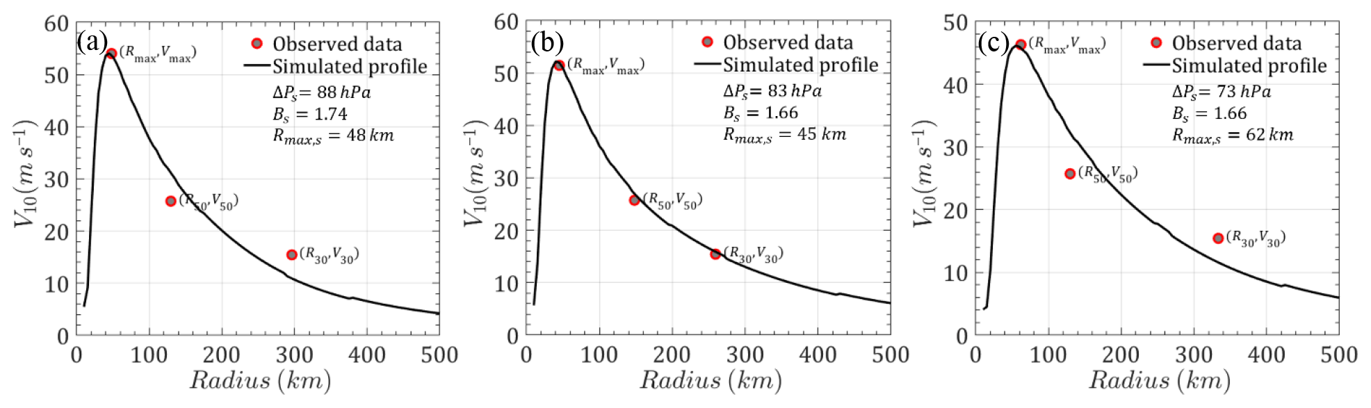
Figure 7 Radial wind speed profiles (a) Saomai (9 August 2006, 15:00 UTC), (b) Parma (1 October 2009, 06:00 UTC) and (c) Rammasun (18 July 2014, 12:00 UTC).

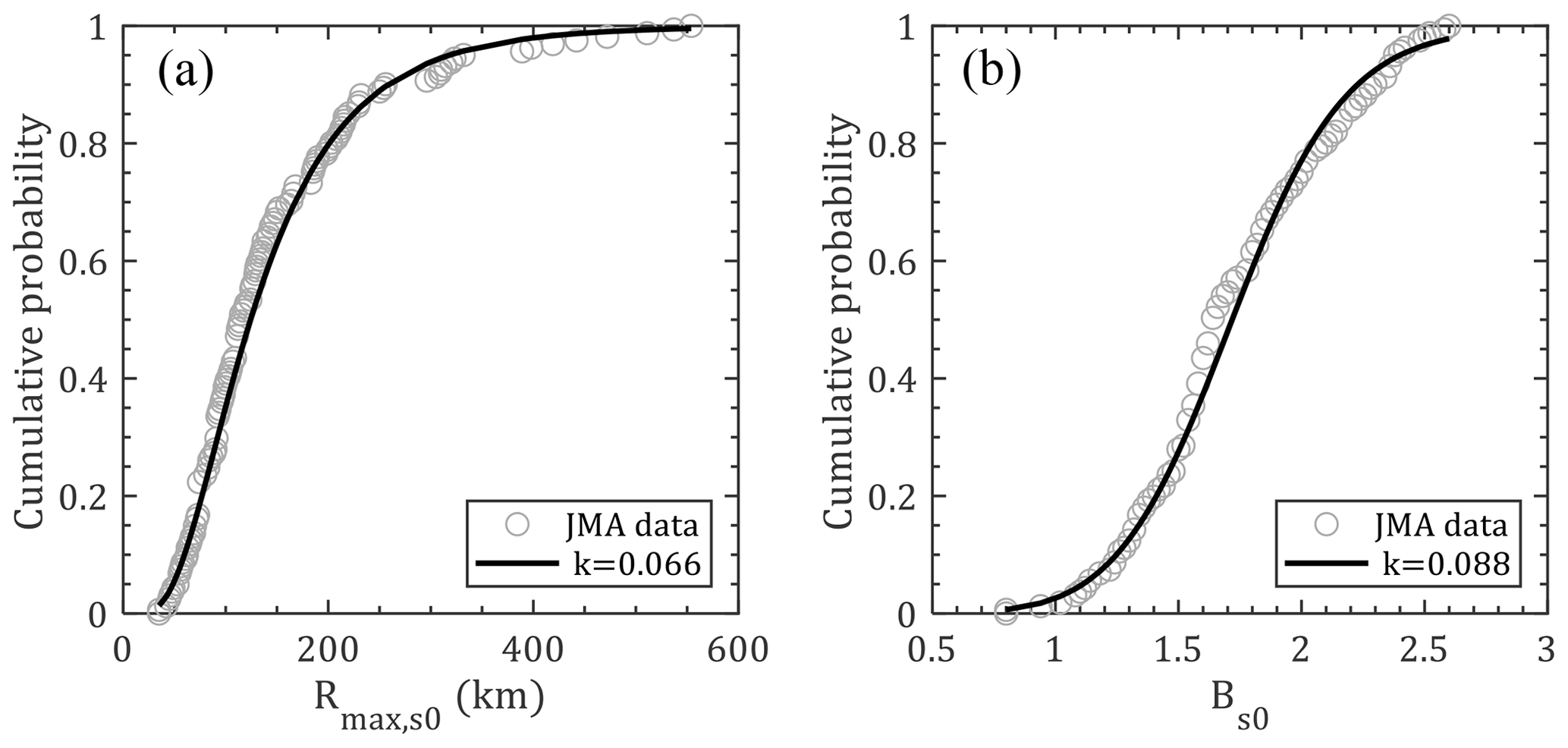
Then, the values of R_max,s0 and B_s0 associated with the track genesis are determined from their probability distributions considering correlations with other parameters. As shown in Fig. 8, R_max,s0 and B_s0 are modeled by lognormal (μ=4.822; σ=0.571) and Burr type XII (α=1.974, c=6.362, k=2.001) distributions, respectively. The critical value of the K–S test (n=161) at a 5 % significance level, say 0.1059, is larger than the test statistics (k values in Fig. 8), which fails to reject the null hypothesis. The correlations of R_max,s0 and B_s0 with other parameters are also introduced and discussed in the next section.

Figure 8 CDFs of wind field parameters at first step: (a) R_max,s0; (b) B_s0.

By using the fitted results from the JMA dataset, the autocorrelations of R_max,s as well as B_s between different time steps are simply taken into account using the recursive models as

$$\begin{array}{}\text{(6)}& {\displaystyle }\begin{array}{rl}\ln R_{\max ,\mathrm{s}}\left(i+\mathrm{1}\right)& =r_{\mathrm{1}}+r_{\mathrm{2}}\cdot \ln R_{\max ,\mathrm{s}}\left(i\right)\\ & +r_{\mathrm{3}}\cdot \ln R_{\max ,\mathrm{s}}\left(i-\mathrm{1}\right)+r_{\mathrm{4}}\cdot \mathrm{\Delta }{P}_{\mathrm{s}}\left(i+\mathrm{1}\right)\\ & +{\mathit{\epsilon }}_{\ln R_{\max ,\mathrm{s}}},\end{array}\text{(7)}& {\displaystyle }\begin{array}{rl}{B}_{\mathrm{s}}\left(i+\mathrm{1}\right)& =b_{\mathrm{1}}+b_{\mathrm{2}}\cdot B_{\mathrm{s}}\left(i\right)+b_{\mathrm{3}}\cdot B_{\mathrm{s}}\left(i-\mathrm{1}\right)\\ & +b_{\mathrm{4}}\cdot \ln R_{\max ,\mathrm{s}}\left(i+\mathrm{1}\right)+b_{\mathrm{5}}\cdot \mathrm{\Delta }{P}_{\mathrm{s}}\left(i+\mathrm{1}\right)\\ & +{\mathit{\epsilon }}_{B_{\mathrm{s}}},\end{array}\end{array}$$

in which r_j (j=1–4) and b_j (j=1–5) are model coefficients that can be fitted with the least-squares regression method, ln R_max,s(i) and B_s(i) are values at time step i, and ${\mathit{\epsilon }}_{\ln R_{\max }}$ and ${\mathit{\epsilon }}_{B_{\mathrm{s}}}$ are error terms accounting for modeling differences between the models and observations. Using the data within the Hong Kong region from 1977 to 2015, the values of r_j (j=1–4) and b_j (j=1–5) are extracted as 0.7039, 0.8341, 0.0282 and −0.0016 and −0.6647, 0.5432, −0.0112, 0.2950 and 0.0013. As illustrated in Fig. 9a and c, there is no obvious bias or potential trend for the error terms of ln R_max,s and B_s with a mean (μ) and standard deviation (σ) of 0 and 0 and 0.29 and 0.20, respectively. Like the translation speed modeled in Sect. 2.3, the error terms of ln R_max,s and B_s are both fitted with normal and t location-scale distributions (Fig. 9b, d). It can be noted that both distributions are good candidates for reconstructing the errors, but t location-scale distribution performs better with smaller K–S values (0.029 and 0.028 for ${\mathit{\epsilon }}_{\ln R_{\max ,\mathrm{s}}}$ and ${\mathit{\epsilon }}_{B_{\mathrm{s}}}$), while the critical value of the K–S test for the observation data sample (n=799) is 0.0478 at a 5 % significance level. The fitted parameters for ${\mathit{\epsilon }}_{\ln R_{\max ,\mathrm{s}}}$ and ${\mathit{\epsilon }}_{B_{\mathrm{s}}}$ with t location-scale distribution are μ=0.0107, σ=0.1470 and ν=2.0340 and μ=0.0054, σ=0.1461 and ν=4.1558, respectively.

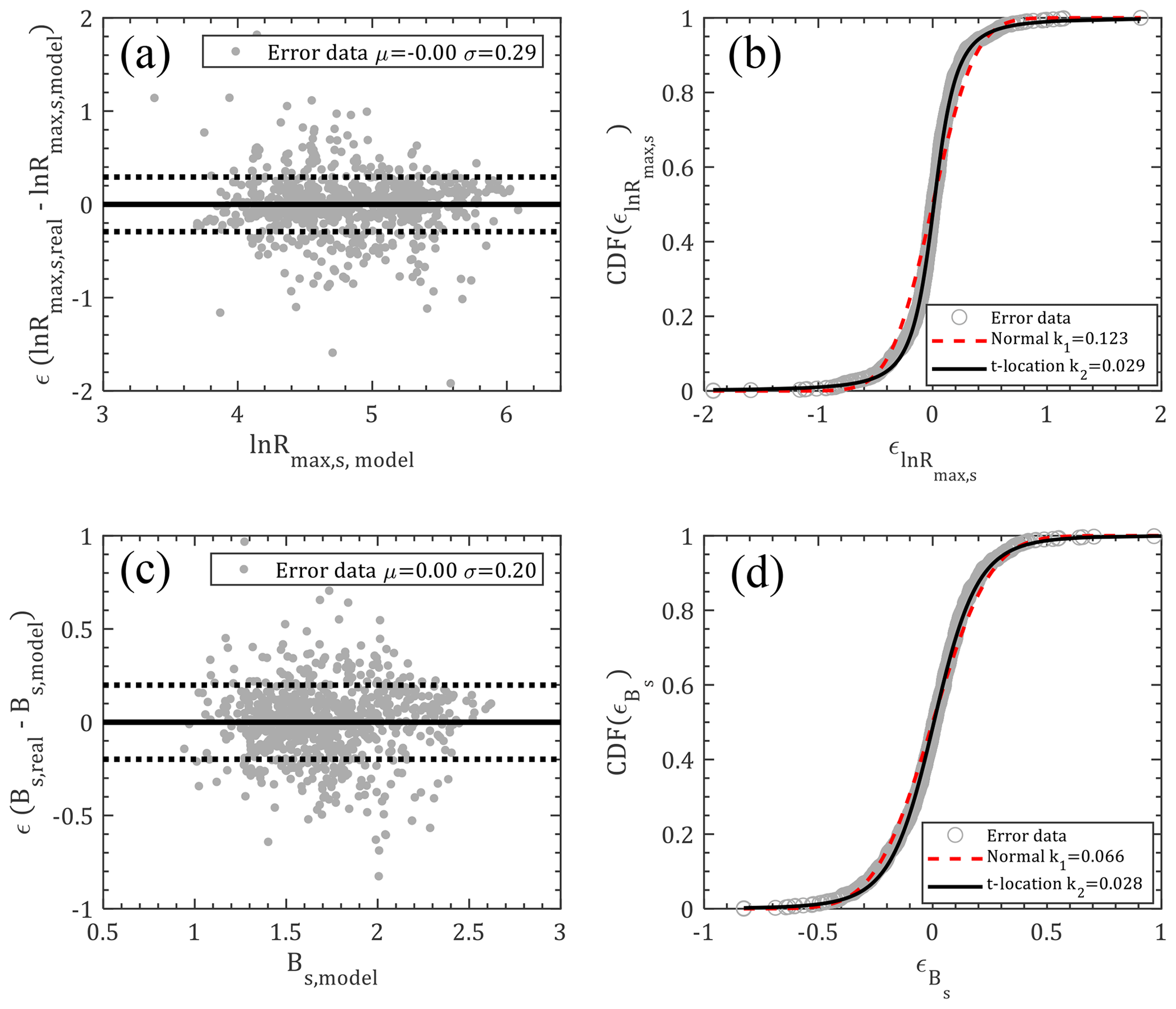
Figure 9 Model errors for ln R_max,s and B_s: (a) scatterplot (${\mathit{\epsilon }}_{\ln R_{\max ,\mathrm{s}}}$); (b) CDF (${\mathit{\epsilon }}_{\ln R_{\max ,\mathrm{s}}}$); (c) scatterplot (${\mathit{\epsilon }}_{B_{\mathrm{s}}}$); (d) CDF (${\mathit{\epsilon }}_{B_{\mathrm{s}}}$).

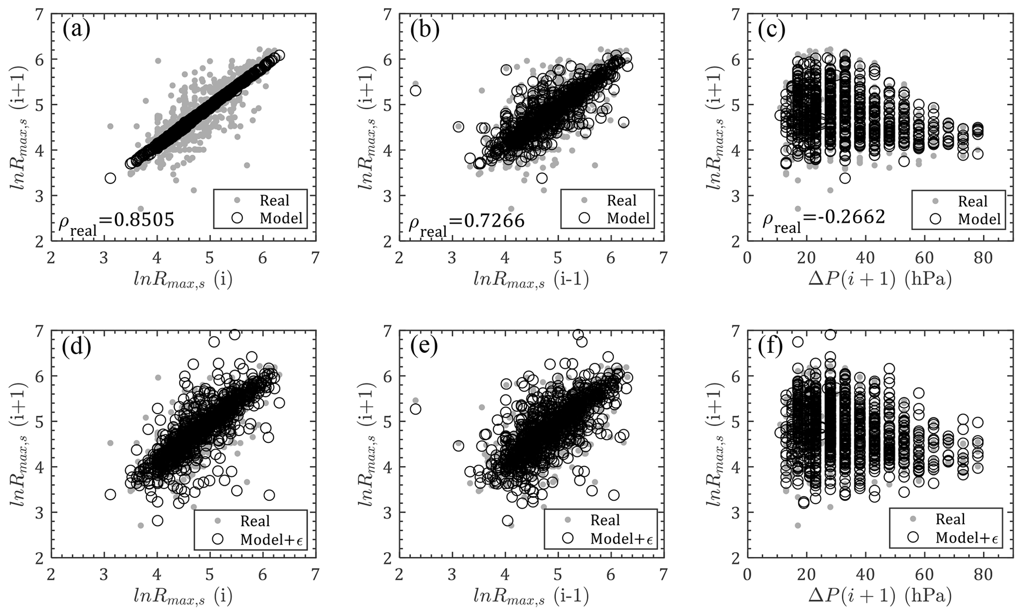
Figure 10 Comparison of ln R_max,s between model and real observations: (a–c) relations between ln R_max,s(i), $\ln R_{\max ,\mathrm{s}}(i-\mathrm{1})$, ΔP(i+1) and $\ln R_{\max ,\mathrm{s}}(i+\mathrm{1})$ without errors; (d–f) relations between ln R_max,s(i), $\ln R_{\max ,\mathrm{s}}(i-\mathrm{1})$, ΔP(i+1) and $\ln R_{\max ,\mathrm{s}}(i+\mathrm{1})$ with errors (ρ_real is the correlation coefficient for real observation data).

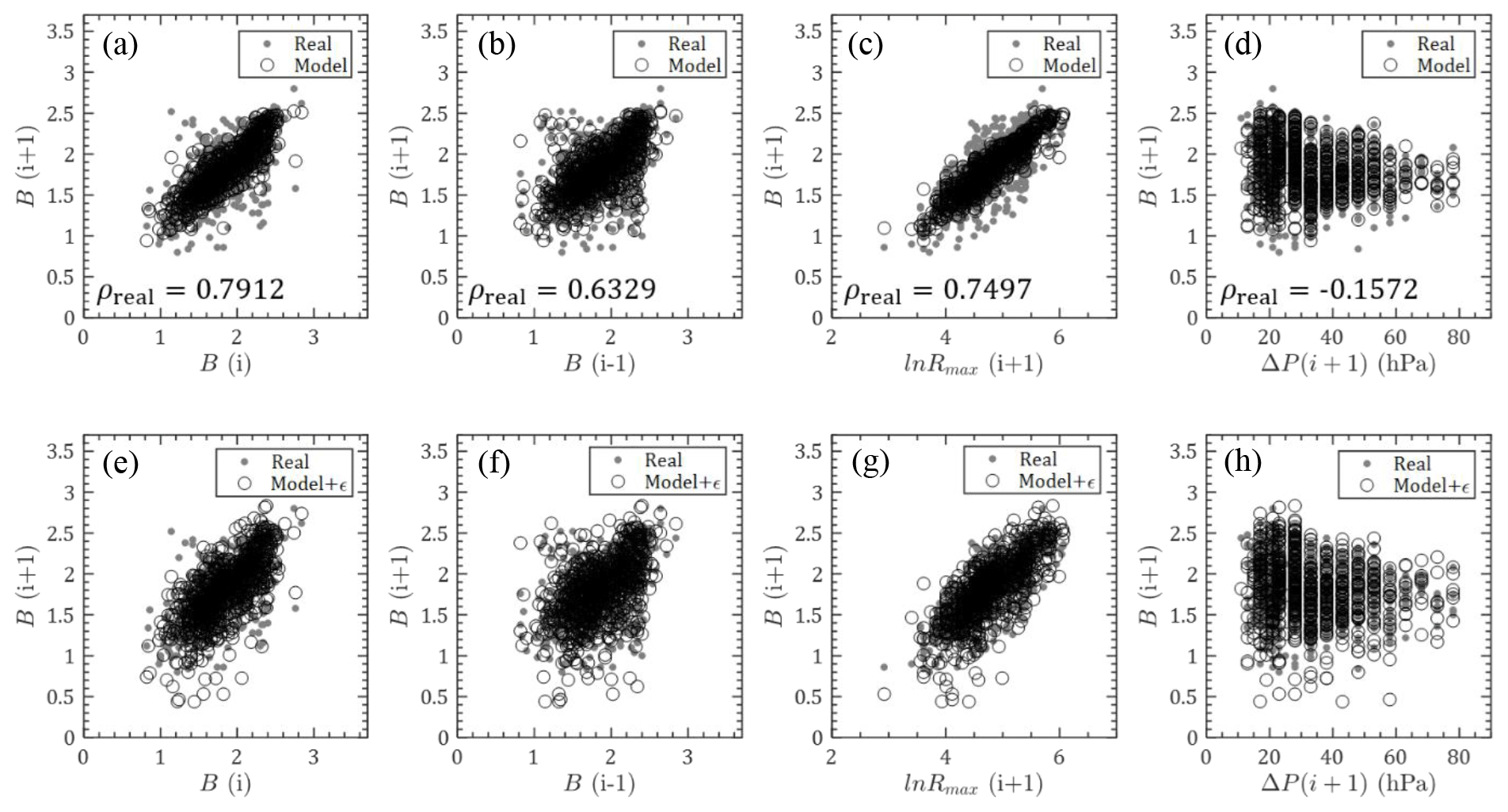
Figure 11 Comparison of B_s between model and real observations: (a–d) relations between B_s(i), B_s(i−1), $\ln R_{\max ,\mathrm{s}}(i+\mathrm{1})$, ΔP(i+1) and B_s(i+1) without errors; (e–h) relations between B_s(i), B_s(i−1), $\ln R_{\max ,\mathrm{s}}(i+\mathrm{1})$, ΔP(i+1) and B_s(i+1) with errors (ρ_real is the correlation coefficient for real observation data).

As shown in Figs. 10–11, R_max,s0 and B_s0 modeled by Eqs. (6) and (7) using the JMA historical data for previous steps are also compared with real observations for next steps. Similarly, the first rows in these two figures ignore the error terms, which are taken into account in the second rows. The values of previous first steps are observed to dominate the model results with linearly concentrated predictions, while previous second steps and other parameters have weaker effects with more scattered model values. After introducing the error terms, model values are able to successfully capture the historical data.

3.3 Decay model

Once the storm makes landfall, the central pressure deficit will witness a sudden decrease due to the cutoff of warm and moist air from the underlying oceanic environment, after which the TC intensity decay model or filling-rate model is adopted. The modeling of storm decay is of great importance for accurately estimating the TC design wind speed at the site of interest since the maximum winds normally occur during storm landfall in most cases. Georgiou (1985) modeled the decay of central pressure as a function of distance after landfall for four regions of the United States based on historical data. The other commonly used filling-rate model (Vickery, 2005) assumes that the central pressure deficit decays exponentially with time after landfall in the form of

$$\begin{array}{}\text{(8)}& \mathrm{\Delta }P\left(t\right)=\mathrm{\Delta }{P}_{\mathrm{0}}\cdot \exp \left(-at\right),\end{array}$$

in which t is the time after landfall (hour), ΔP₀ is the central pressure difference at landfall (hPa), and a is called the decay rate, which is correlated with ΔP₀ and modeled as

$$\begin{array}{}\text{(9)}& a=a_{\mathrm{1}}+a_{\mathrm{2}}\mathrm{\Delta }{P}_{\mathrm{0}}+{\mathit{\epsilon }}_a,\end{array}$$

where a₁ and a₂ are two region- and topographic-dependent coefficients, and ε_a is a zero-mean normally distributed error term. As shown in Fig. 12a, the decay information of the ratio of central pressure deficit was extracted from the landfall TCs in the circular region around Hong Kong (Fig. 2) and fitted with the decay model of Eq. (8) using a least-squares analysis. Generally, the decay model is well behaved although it is unable to capture the unchanged central pressures with time after landfall. This is also discussed in detail by Vickery (2005). Furthermore, the correlation between decay rate and central pressure difference at landfall is plotted in Fig. 12b with the correlation coefficient ρ=0.3019, which is also modeled by the linear function of Eq. (9). Then the residual error is unbiased and can be modeled by a normal distribution with a mean and standard deviation of 0 and 0.0227, respectively.

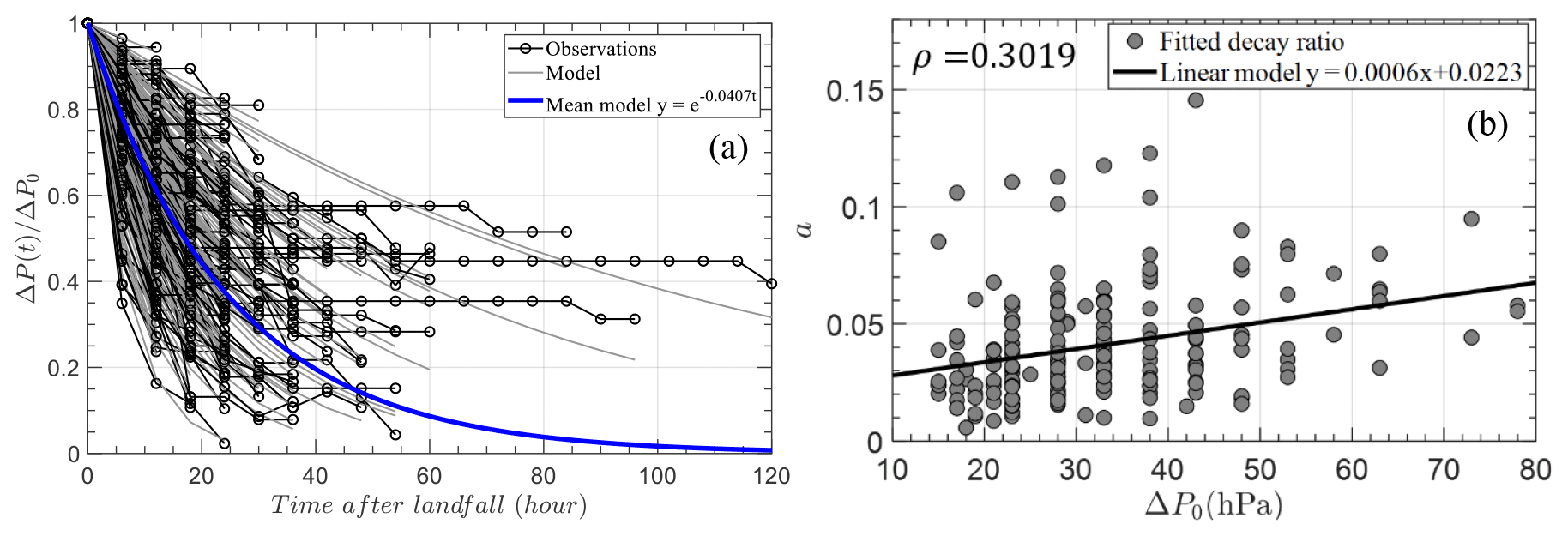
Figure 12 Decay model in circular subregion around Hong Kong: (a) curve fitting of decay model; (b) decay rate versus ΔP₀.

4 TC design wind speed prediction

4.1 Parameter correlations

As shown by the scatterplots in Fig. 13, the observed (red triangles) genesis (at first time step) parameters show some correlations, especially between θ₀ and α₀ and between R_max,s0 and B_s0 with correlation coefficients larger than 0.5. This means that the heading direction at the first time step is dependent on genesis location and two wind field parameters are strongly correlated with each other. Accordingly, the correlations between these genesis parameters, i.e., α₀, ΔP₀, θ₀, V_T0, R_max,s0 and B_s0, should be considered when utilizing the Cholesky decomposition method, which is a distribution-free approach introduced by Iman and Conover (1982). The randomly generated independent variables can be written into a matrix of size N×6 (N is the number of simulation samples) as

$$\begin{array}{}\text{(10)}& \mathbf{X}=\left[{\mathit{\alpha }}_{\mathrm{0}},\mathrm{\Delta }{P}_{\mathrm{0}},{\mathit{\theta }}_{\mathrm{0}},V_{\mathrm{T}\mathrm{0}},R_{\max ,\mathrm{s}\mathrm{0}},B_{\mathrm{s}\mathrm{0}}\right].\end{array}$$

The correlation coefficients of real data are assembled into a positive definite and symmetric matrix of C. It can be alternatively expressed as C=AA^T using the Cholesky decomposition method, in which A is a lower triangular matrix. If the correlation matrix of X is Q, it can also be decomposed into the product of a lower triangular matrix P and its transpose P^T; i.e., Q=PP^T. A matrix $\mathbf{S}={\mathbf{AP}}^{-\mathrm{1}}$ can be determined such that SQS^T=C. After that, the final transformed correlated matrix X_c=XS^T can be obtained, which has the desired correlation matrix C. It is noteworthy that the values in each column of the input N×6 matrix X can be rearranged to have the same rank order as the target matrix.

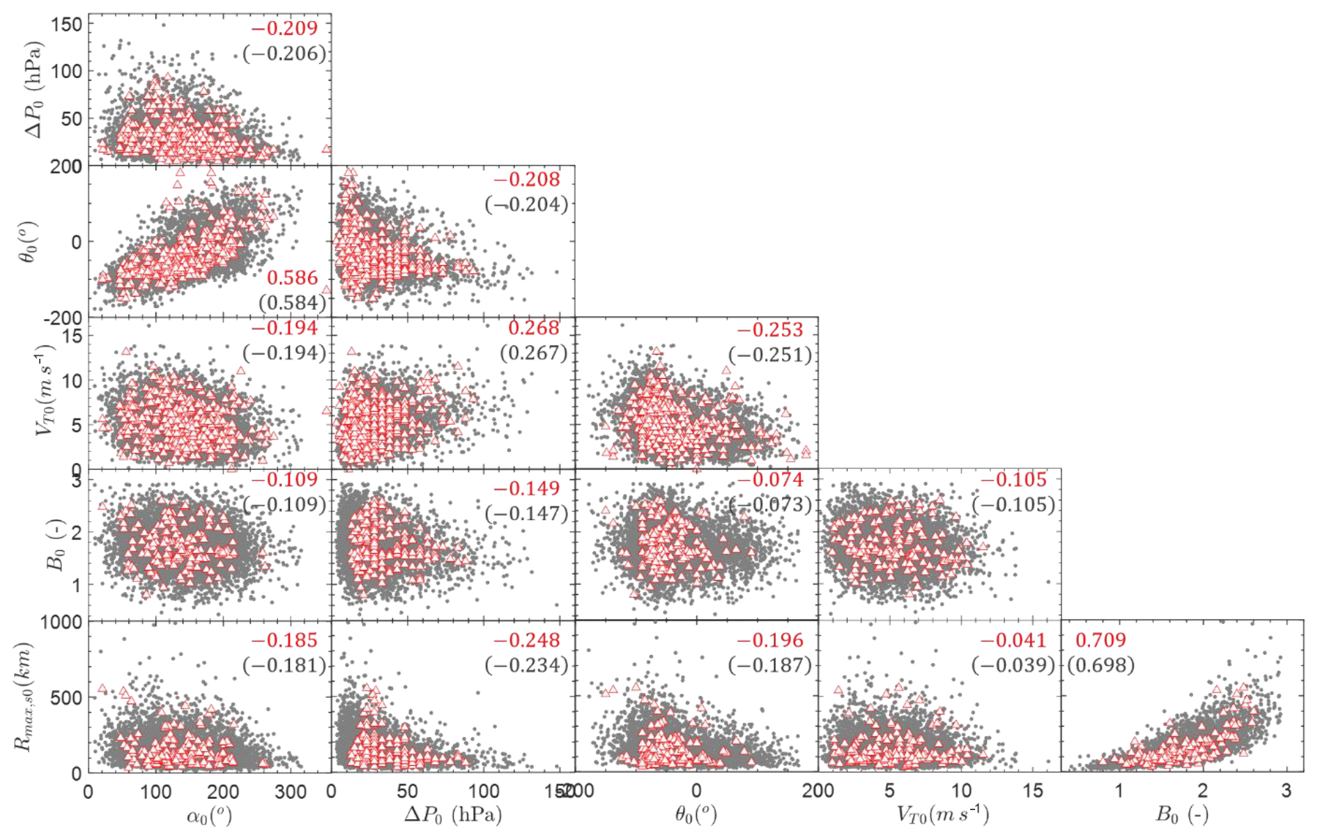
Figure 13 Simulated and observed genesis parameters (red triangles: observations; grey dots: simulations; upper numbers: ρ_sim; lower numbers in parentheses: ρ_obs).

The correlated genesis samples for 100 years for Hong Kong are generated by Monte Carlo simulations coupled with parameter correlation analysis, as shown in Fig. 13. As can been seen, the observed JMA data points are scattered around the simulated results. And the correlation coefficients of the simulated variables (ρ_sim) are almost identical to those of the original observations (ρ_obs). It is worth mentioning that the historical data for α₀, ΔP₀, θ₀ and V_T0 are more than those for R_max,s0 and B_s0 since the wind speed information is only available from 1977 and the wind data estimations are usually not provided during the first and last several time steps of a TC track due to its weak intensity. As a result, the scatterplots for historical observations in Fig. 13 associated with R_max,s0 and B_s0 contain fewer data than others. Correspondingly, the correlation coefficients associated with these two parameters would also be derived from fewer data.

4.2 Design wind speed prediction

After generating the virtual tracks as well as the wind field parameters, the TC wind speed at the site of interest can be readily solved using the wind speed field model. Then, our final objective is to investigate the design wind speeds with various return intervals or TC wind hazard curves for the site of interest. For each site, 10 000-year simulations should be conducted to achieve adequate TC samples. The underlying terrain exposure is assumed to be consistent with the standard condition specified by the Load Code for the Design of Building Structures (GB-50009 2012; China National Standard, 2012), i.e., flat, open and low-density residential area of terrain category B with equivalent roughness length z₀=0.05 m. These simulated tracks can also be employed to estimate the wind speed with respect to other underlying exposures by simply using a desired input of z₀. And all simulated tracks can be interpolated into 15 min so as to capture every potential maximum wind speed.

By assuming that the number of TCs occurring in a given season is independent of any other season, the occurrence probability P_T(n) of n TCs over the time period T can be assumed to follow the Poisson distribution. Then, the probability that the extreme wind speed v_i is larger than a certain wind speed V within a time period T can be determined as

$$\begin{array}{}\text{(11)}& \begin{array}{rl}{P}_{\mathrm{T}}\left(v_i>V\right)& =\mathrm{1}-\sum _{n=\mathrm{0}}^{\mathrm{\infty }}P\left(v_i\le V\mathrm{|}n\right)P_{\mathrm{T}}\left(n\right)\\ & =\mathrm{1}-\exp \left(-{\displaystyle \frac{N}{Y}}T\right),\end{array}\end{array}$$

in which P(v_i≤V|n) is the probability that the peak wind speed v_i of a given TC is less than or equal to V, N is the total number of TCs of which each has a peak wind v_i larger than V, and Y is total simulation years. Defining T=1 year, the annual probability of exceeding a given wind speed V is

$$\begin{array}{}\text{(12)}& \begin{array}{rl}{P}_{\mathrm{T}}& =\mathrm{1}\mathrm{year}\left(v_i>V\right)=\mathrm{1}-\exp \left[-\mathit{\lambda }P\left(v_i>V\right)\right]\\ & =\mathrm{1}-\exp \left(-{\displaystyle \frac{N}{Y}}\right),\end{array}\end{array}$$

in which λ is the annual storm occurrence rate within the region of interest. The mean recurrence interval (MRI) or return period (RP) of a given wind speed V at a specific site can be estimated using the inverse of the result of Eq. (12) with the form

$$\begin{array}{}\text{(13)}& \mathrm{RP}\left(v_i>V\right)={\displaystyle \frac{\mathrm{1}}{\mathit{\lambda }P\left(v_i>V\right)}}={\displaystyle \frac{Y}{N}}.\end{array}$$

Figure 14 illustrates the empirical distribution of the annual maximum TC mean wind speeds (10 min duration at 10 m height) curve as well as the return period curve of design mean wind speed in Hong Kong. Although the lognormal distribution is adopted for ΔP₀ in this study, a similar distribution trend of annual maximum TC mean wind speed can be observed in this study and Li and Hong (2015) when ΔP is modeled by a Weibull distribution (Fig. 14a). A Weibull distribution was also preferred to the lognormal distribution in their study. However, the lognormal distribution is the preferred distribution in this study. This is mainly attributed to the use of different historical track datasets and a different subregion size. Li and Hong (2015) adopted the best-track dataset from the China Meteorological Agency and a radius of 250 km for the subregion circle. Thus, modeling the historical data with preferable probabilistic distributions is essentially important before the estimation of TC design wind speed can be regarded as a site-specific issue.

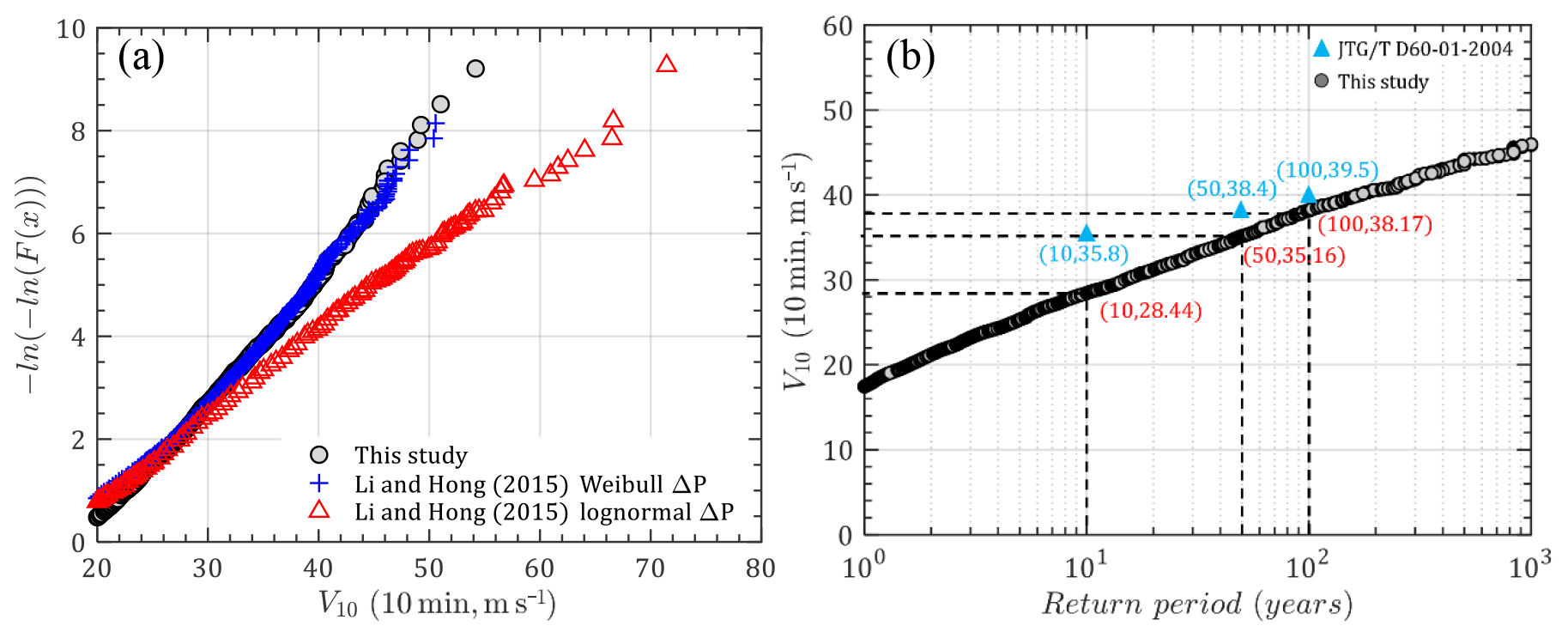
Figure 14 Design mean wind speed in Hong Kong: (a) empirical distribution; (b) mean wind speed versus return periods.

Moreover, Fig. 14b compares the predicted design mean wind speeds with the recommended values in Wind-resistant Design Specification for Highway Bridges (JTG/T D60-01-2004, code hereafter; China Trade Standard, 2004) for different return periods. It can be noted that the code's values are larger than those obtained in this study and the difference seems to decrease with an increase in return period. This is because the values recommended in the code are developed by statistical approaches based on both TC and non-TC observations over 30–40 years. Some strong non-TC winds captured by meteorological stations could dominate the design values for short return periods, while strong TC winds would control the higher design wind speed corresponding to longer return periods.

As mentioned in the explanatory materials to the Hong Kong Code (Buildings Department, 2004a, b), the 50-year MRI hourly mean wind speed of 46.9 m s⁻¹ at 90 m above mean sea level with the underlying exposure of open sea was selected as the reference. In this case, the 10 m wind speed is estimated as 36.83 m s⁻¹ using the power wind profile with the suggested exponent of 0.11 (0.12 for terrain exposure A in the Chinese code, 1∕9 for terrain exposure D in ASCE 7-16). The estimated 10 min mean wind speed is roughly 39.04 m s⁻¹ if the conversion factor is 1.06 from 1 h to 10 min. However, in order to be consistent with the reference exposure in this study (z₀=0.05), the gradient wind speed can be determined as 56.64 m s⁻¹ at 500 m and is assumed to be the same as other exposures. Then, the 10 min wind speed at a height of 10 m associated with open flat terrain can be calculated as 33.39 m s⁻¹ if the power exponent is 0.15 (0.16 for terrain exposure B in the Chinese code, 1∕6.5 for terrain exposure C in ASCE 7-16) and the same gradient height is employed. This value is about 2 m s⁻¹ smaller than the result of this study (35.16 m s⁻¹). Similar results can be found from Kwok et al. (2006), who summarized that the over-sea wind speed at a height of 500 m with an MRI of 50 years was within the range of 54–57 m s⁻¹ based on the historical TC records and recommended a slightly higher value of 59.5 m s⁻¹ for design purposes. The corresponding 10 min mean wind speed associated with z₀=0.05 is estimated to be 35.07 m s⁻¹ by following the same algorithm, which compares favorably to the result in the present study. Accordingly, the predicted design wind speed in Hong Kong in this study has an expected level of confidence for engineering applications.

4.3 TC wind hazards at selected coastal cities in China

For comparison with other studies (Xiao et al., 2011; Li and Hong, 2015), nine other coastal cities (Fig. 15), i.e., Shanghai, Ningbo, Wenzhou, Fuzhou, Xiamen, Guangzhou, Shenzhen, Zhanjiang and Haikou, were selected for Monte Carlo simulations following the aforementioned algorithm. Because the Burr distribution fails to fit the empirical B_s0 in Shanghai, Ningbo and Wenzhou, the generalized extreme value (GEV) distribution was employed to model B_s0 of these three cities. GEV distribution is a commonly used distribution developed from extreme value theory to combine the Gumbel, Fréchet and Weibull function families, also known as types I, II and III extreme value distributions. Its PDF can be expressed as

$$\begin{array}{}\text{(14)}& {\displaystyle }\begin{array}{rl}f\left(x;\mathit{\mu },\mathit{\sigma },\mathit{\gamma }\right)& ={\displaystyle \frac{\mathrm{1}}{\mathit{\sigma }}}\exp \left[-{\left(\mathrm{1}+\mathit{\gamma }\cdot {\displaystyle \frac{x-\mathit{\mu }}{\mathit{\sigma }}}\right)}^{-\frac{\mathrm{1}}{\mathit{\gamma }}}\right]\\ & {\left(\mathrm{1}+\mathit{\gamma }\cdot {\displaystyle \frac{x-\mathit{\mu }}{\mathit{\sigma }}}\right)}^{-\mathrm{1}-\frac{\mathrm{1}}{\mathit{\gamma }}},\mathit{\gamma }\ne \mathrm{0},\end{array}\text{(15)}& {\displaystyle }\begin{array}{rl}f\left(x;\mathit{\mu },\mathit{\sigma },\mathrm{0}\right)& ={\displaystyle \frac{\mathrm{1}}{\mathit{\sigma }}}\exp [-\exp \left(-{\displaystyle \frac{x-\mathit{\mu }}{\mathit{\sigma }}}\right)\\ & -{\displaystyle \frac{x-\mathit{\mu }}{\mathit{\sigma }}}],\mathit{\gamma }=\mathrm{0},\end{array}\end{array}$$

in which γ, σ and μ are called shape, scale and location parameters, respectively, and $\mathrm{1}+\mathit{\gamma }(x-\mathit{\mu })/\mathit{\sigma }>\mathrm{0}$. Correspondingly, for γ=0, γ>0 and γ<0 conditions, GEV distributions can be reduced to types I, II and III extreme value distributions. As shown in Tables 2–3, coefficients of each distribution for various input parameters in another nine coastal cities of China were estimated using a maximum likelihood method based on historical observation around the site of interest within a radius of 500 km. The annual storm rate was observed to gradually increase from north to south. The fitted coefficients of recursive models of V_T, R_max,s and B_s as well as the decay model coefficients are also listed in Table 3. Correspondingly, the empirical and fitted preferred CDFs for each parameter in nine cities are illustrated in Fig. 16 together with the K–S test statistics. It can be seen that the distribution models successfully matched the empirical historical samples.

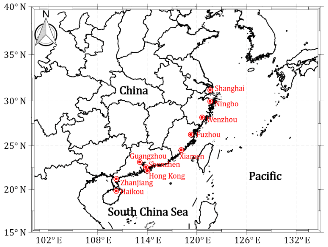
Figure 15 Locations of 10 selected coastal cities in China.

Table 2 Coefficients of PDFs for TC track genesis parameters.

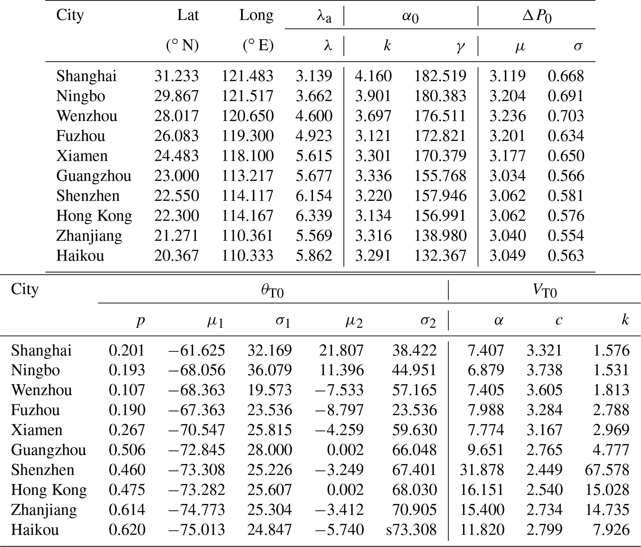
Table 3 Coefficients of PDFs and recursive models for wind field parameters.

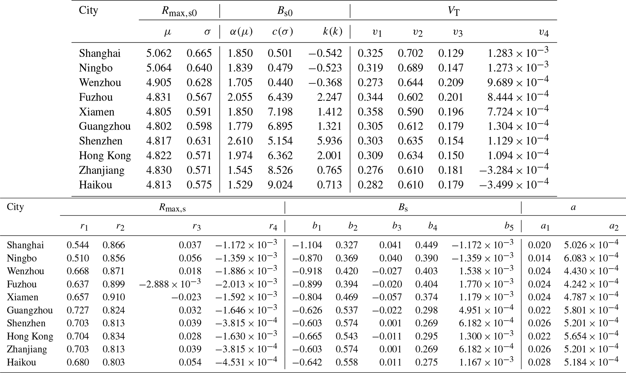
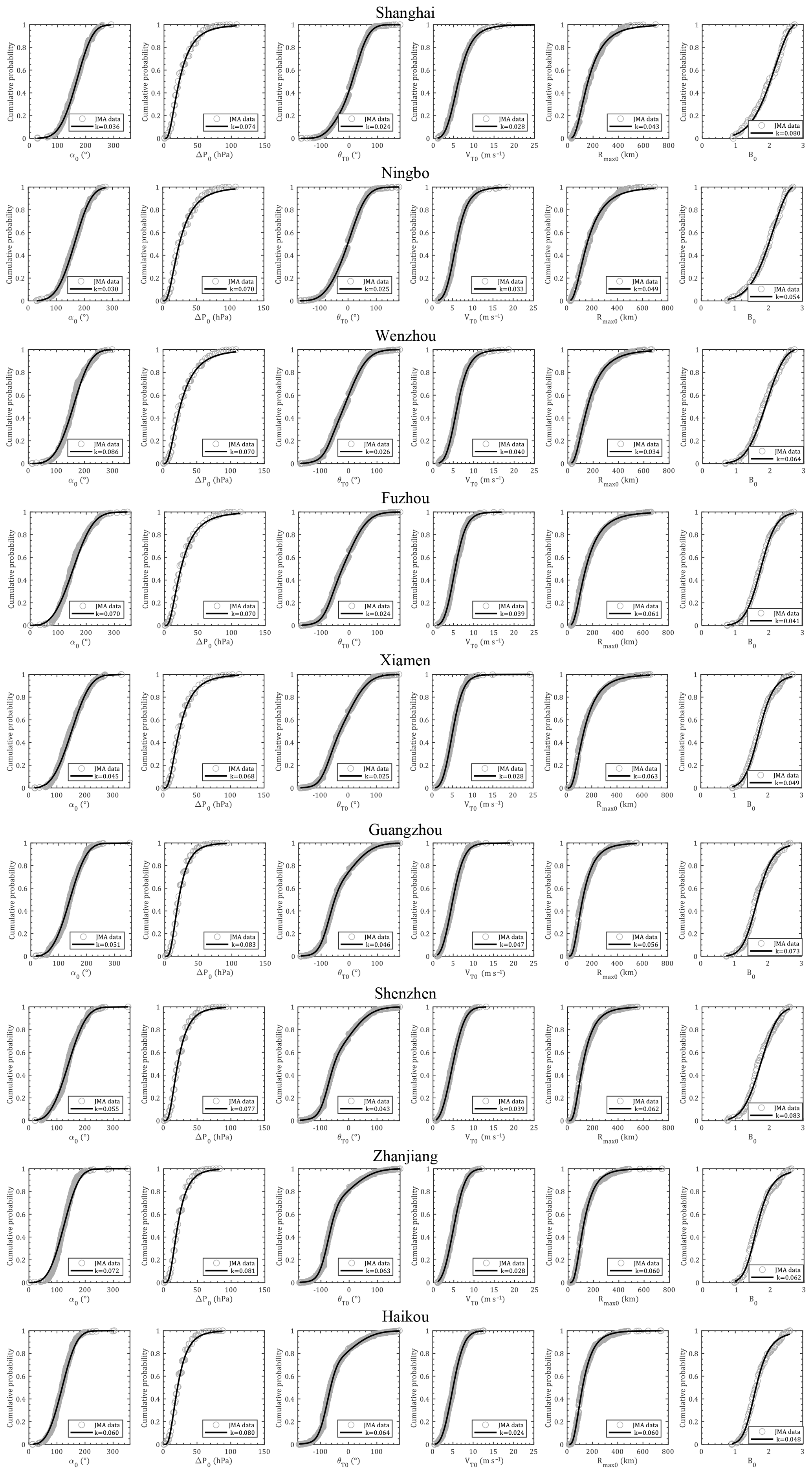
Figure 16 Empirical and preferable cumulative probability distributions for α₀, ΔP₀, θ₀, V_T0, R_max,s0 and B_s0.

Like Hong Kong, the 10 min mean design wind speeds at a height of 10 m above the ground with a surface roughness of 0.05 m with respect to various return periods were developed based on 10 000-year Monte Carlo simulations. Table 4 lists the simulation results for TC design wind speed at selected cities with an MRI of 100 years and compares them with two Chinese codes (JTG/T D60-01-2004; GB 50009-2012) as well as other pioneering studies. The design wind speeds in the two codes are consistent with each other, except for a 2.5 m s⁻¹ difference in Shanghai. It can be seen that the predicted wind speeds in this study are close to the code-recommended values, except for in Ningbo, Wenzhou, Zhanjiang and Haikou. The estimated values for Ningbo and Wenzhou are more than 4 m s⁻¹ higher than those in the codes, while those for Zhanjiang and Haikou are more than about 4 m s⁻¹ smaller. A similar trend can also be observed from the differences between Li and Hong (2016), Chen and Duan (2018), Wu and Huang (2019), and the codes. This is mainly attributed to the limitations of the statistically short-term data-based method used in the code development. As mentioned before, the design wind speeds in the Chinese codes are developed from short-term observations utilizing both TC and non-TC winds (30–40 years). However, the series of largest annual wind speeds are, in most cases, not well behaved (Simiu and Scanlan, 1996) when used for modeling the probabilistic behavior of the extreme winds since most of the largest annual winds are remarkably smaller than the extreme winds associated with TCs. That is, the contribution of each group of data used for characterizing the probabilistic behavior of the largest annual winds is uneven, resulting in some unrealistically high or low predictions (Simiu and Scanlan, 1996). Although some alternative approaches can be adopted to better consider TC winds, such as the use of maximum average monthly speed or mixed distributions of TC and non-TC winds, to the authors' knowledge, no published literature clearly discusses the development of design wind speed in the Chinese codes. Furthermore, the correction of averaging time, height, station migration and surrounding roughness to make the wind speed records meteorologically homogeneous would introduce some unpredictable errors.

Table 4 Comparison of TC design wind speed at selected cities (MRI =100 years; T=10 min; z=10 m, z₀=0.05 m; m s⁻¹).

Figure 17 Strong typhoon tracks affect Ningbo, Wenzhou, Hong Kong and Zhanjiang: (a) violent typhoons (P_c<935 hPa or V_max>57 m s⁻¹); (b) strong typhoons (P_c<960 hPa or V_max>43 m s⁻¹).

Moreover, as shown in Fig. 17, violent typhoons (P_cs≤935 hPa or $V_{\max ,\mathrm{s}}\ge \mathrm{54}$ m s⁻¹, 105 knots) as well as strong typhoons (P_cs≤960 hPa or $V_{\max ,\mathrm{s}}\ge \mathrm{44}$ m s⁻¹, 85 knots), that affect Zhanjiang (close to Haikou), Hong Kong (close to Shenzhen), Wenzhou and Ningbo within 500 km are extracted from the 65-year JMA dataset. It turns out that only two TCs (200814 Hagupit and 201409 Rammasun) around Zhanjiang (or Haikou) and six TCs (195408 Ida, 197909 Hope, 200814 Hagupit, 201013 Megi, 201319 Usagi and 201409 Rammasun) around Hong Kong (or Shenzhen) reached the violent level. Comparatively, 25 and 13 violent typhoons were observed around Wenzhou and Ningbo, respectively. Moreover, 40 and 52 strong typhoons affected Zhanjiang and Hong Kong, respectively, while Wenzhou and Ningbo suffered 89 and 55 strong typhoons over the past half a century. This is thanks to the obstacle effects of several high mountains in the Philippines so that the violent typhoons making landfall in Hainan and Guangdong provinces usually need to reintensify in the South China Sea or directly pass through the Bashi Channel between Taiwan and the Philippines, so not many violent typhoons were observed to affect these two provinces. In addition, the maximum wind of the rotating storm in the Northern Hemisphere always occurs on its right side with respect to the heading direction due to the Coriolis effect. Thus, westward-heading violent typhoons seldom occur in Zhanjiang and Haikou before their intensities decay due to the effect of Hainan island. Instead, Hong Kong, Wenzhou or Ningbo have greater chances of being swept by a storm's maximum wind. Accordingly, the prediction results should be more reasonable with higher design wind speeds in Wenzhou and Ningbo than in Zhanjiang and Haikou. It is suggested that this trend should be validated in a future study using more TC observation data.

The results in Xiao et al. (2011) are higher than those in other studies or codes. There are three possible reasons for this. The first is the use of the Holland (2008) method in determining B values. This method was developed from semiempirical relationships between the gradient and surface layer as discussed by Fang et al. (2018a). Another reason is the use of a 1000 km radius subregion, which would take into account many extremely violent typhoons over the distant sea before they are used for TC intensity modeling. The third one is the use of a surface roughness of 0.02 m, which is smaller than the code-specified value associated with the terrain exposure B of 0.05 m.

The estimated wind speeds in Shanghai, Ningbo and Wenzhou are 2–3 m s⁻¹ higher than the equivalents in Li and Hong (2016), while Zhanjiang showed about a 7 m s⁻¹ smaller result. The other five cities show a satisfactory comparison between results of this study and those of Li and Hong (2016). When they are compared with Chen and Duan (2018), who used an improved full-track model, the present estimations in Zhanjiang and Haikou are also about 4 m s⁻¹ smaller, while the other cities show 1–4 m s⁻¹ higher values. Except for the potential reasons analyzed above, it is worth mentioning that Li and Hong (2016) adopted CMA track data with a 2 min duration while Chen and Duan (2018) used a JTWC dataset with a 1 min duration. Some errors could be introduced by the time duration gaps for different datasets. The wind speeds predicted by Wu and Huang (2019) are similar to those estimated by Li and Hong (2016), which is mainly attributed to the use of the same best-track dataset as well as R_max and B models.

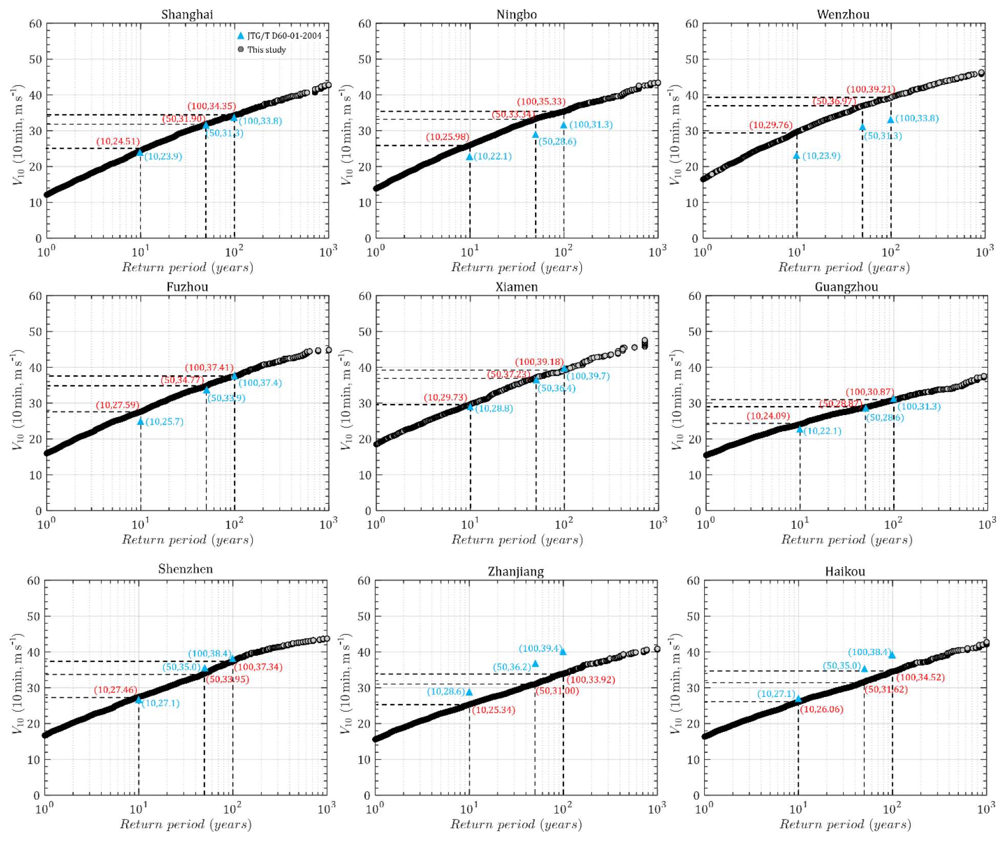
Figure 18 Predicted and code-suggested TC design wind speed versus return period of nine coastal cities in China.

Figure 18 illustrates design wind speed versus return period plots (hazard curves) based on simulations together with the suggested values in Chinese codes (JTG/T D60-01-2004) for nine coastal cities. It can be seen that the predicted curves for Shanghai, Fuzhou, Xiamen, Guangzhou and Shenzhen are in satisfactory agreement with code suggestions. But, consistent with previous findings, this study shows higher estimations for Ningbo and Wenzhou, while it shows smaller estimations for Zhanjiang and Haikou than the code. It is also found that the estimated hazard curves for Ningbo and Wenzhou have a similar trend to the code, but the design wind speeds for Zhanjiang and Haikou increase more gently with return period than the code provisions. This is closely related to the portion of TC wind samples as well as their contributions to the description of the probabilistic distribution of extreme winds in a series of largest observed annual winds as discussed above. The TC winds in Ningbo and Wenzhou could dominate the probabilistic behavior of the yearly highest wind speed, while Zhanjiang and Haikou have lower portions of TC winds compared to non-TC winds. However, the contributions of strong TC winds will be overused in modeling the hazard curve when they are combined with smaller non-TC winds in the yearly largest wind series. More observations on TC winds and unique descriptions of the probabilistic behavior of TC winds are necessary to model site-specific TC hazards and validate the long-term hazard predictions in this study.

5 Conclusions

The statistical characteristics of TC track as well as wind field parameters within a site-specific circular subregion extracted from the JMA best-track dataset were examined before developing TC wind speed hazard curves for 10 coastal cities in China using a height-resolving wind field model and a Monte Carlo technique. Some improvements and new findings are summarized as follows:

1. Recursive models are applied for both track (translation speed) and wind field (R_max,s and B_s) parameters, which enable the movement as well as the size and wind field scale of a TC to vary smoothly. R_max,s and B_s of the historical dataset are determined from the present height-resolving wind field model coupled with 10 min duration wind information provided by the JMA. Thus, the present study is self-adaptive, and no other statistical models of wind field parameters, which are commonly used in combination in other studies, are adopted. Meanwhile, the documented R_max,s and B_s dataset facilitates the completeness of correlation studies between various parameters at first time steps before generating statistically correlated parameters using the Cholesky decomposition method.

2. The probabilistic behavior of TC track and wind model parameters of the first time steps (genesis parameters) within a 500 km circular subregion of 10 coastal cities is investigated and modeled with some preferable probability distribution models. Then the coefficients of the decay model as well as the recursive models for translation speed, R_max,s and B_s in these 10 cities are also fitted.

3. The TC design wind speed versus return period plots (hazard curve) are developed from 10 000-year Monte Carlo simulations and compared with code suggestions as well as other studies. It is found that the predicted wind speeds in northern cities (Ningbo and Wenzhou) are higher than code suggestions, while those of southern cities (Zhanjiang and Haikou) are smaller. The other six cities show satisfactory agreement with code provisions. Some potential reasons for this are discussed to emphasize the importance of independently developing hazard curves of TC and non-TC winds.