Satellite hydrology observations as operational indicators of forecasted fire danger across the contiguous United States

Traditional methods for assessing fire danger often depend on meteorological forecasts, which have reduced reliability after ∼10 d. Recent studies have demonstrated long lead-time correlations between pre-fire-season hydrological variables such as soil moisture and later fire occurrence or area burned, yet the potential value of these relationships for operational forecasting has not been studied. Here, we use soil moisture data refined by remote sensing observations of terrestrial water storage from NASA's Gravity Recovery and Climate Experiment (GRACE) mission and vapor pressure deficit from NASA's Atmospheric Infrared Sounder (AIRS) mission to generate monthly predictions of fire danger at scales commensurate with regional management. We test the viability of predictors within nine US geographic area coordination centers (GACCs) using regression models specific to each GACC. Results show that the model framework improves interannual wildfire-burned-area prediction relative to climatology for all GACCs. This demonstrates the importance of hydrological information to extend operational forecast ability into the months preceding wildfire activity.

1 Introduction

Fires are a key disturbance globally, acting as a catalyst for terrestrial ecosystem change and contributing significantly to both carbon emissions (Page et al., 2002) and changes in surface albedo (Randerson et al., 2006). Furthermore, the socioeconomic impact of fires includes human casualties as tremendous economic loss across the United States. For example, the year 2018 was the largest fire year on record, resulting in approximately USD 3 billion in suppression costs (https://www.nifc.gov/fireInfo/fireInfo_documents/SuppCosts.pdf; last access: 17 April 2020). Several studies have shown that in the western United States, fires have demonstrated a positive trend in annual area burned that will likely continue into the future (Littell et al., 2010; Stavros et al., 2014b). In response to increasing annual area burned and detrimental losses, the US Forest Service has increased funding for active fire management from 16 % to 52 % of their total budget that would have otherwise been spent on land management and research (USFS, 2015). These increased costs translate directly to increased USFS (United States Forest Service) information needs because any intra- or interannual early warning helps decrease the cost of preparing for, managing and, when necessary, suppressing fires that occur.

The severe consequences of wildfires motivate the need for capabilities to map fire potential on timescales ranging from days to months. Operational fire management agencies rely on two primary sources of information to predict fire danger: meteorological forecasts and expert judgment (e.g., https://www.predictiveservices.nifc.gov/outlooks/outlooks.htm; last access: 17 April 2020). Fire danger forecasts are generally reported in the form of qualitative categories (e.g., normal, below-normal and above-normal). Such categories are used by the US National Interagency Fire Center (NIFC) to allocate fire management resources across jurisdictional boundaries (e.g., state or national) when local response capabilities are exhausted. These qualitative metrics are derived from many information layers including fire danger indices.

Fire danger indices (e.g., the US National Fire Danger Rating System – NFDRS; Bradshaw et al., 1984) typically use meteorological input (Abatzoglou and Brown, 2012; Holden and Jolly, 2011) that is sometimes not available with the long lead time needed for regional, transboundary fire management planning. Gridded meteorological data often have several limitations. The data are interpolated between weather stations (Daly et al., 2008); developed by combing spatial and temporal attributes of different climate data and validated with weather stations (Abatzoglou, 2013; Abatzoglou and Brown, 2012); or provided by meteorological reanalysis, i.e., numerical weather prediction models that assimilate weather station data (Kalnay et al., 1996; Roads et al., 1999). These weather stations are sometimes far away from the location of interest and do not always provide good estimates of local climate, especially in complex topography. Moreover, forecasts beyond 10 d for a given landscape location have low skill (Bauer et al., 2015). The mentioned limitations of current operational fire danger systems result in the need for additional information that could help improve predictions of fire danger at monthly intervals and help allocate resources across the country as the active fire season progresses and resources become strained. This added information could result in less subjective and more accurate fire danger forecasts for larger areas and for timescales of a month or longer.

A number of previous studies have demonstrated relationships between fire and hydrological indicators (Parks et al., 2014; Shabbar et al., 2011; Westerling et al., 2002; Xiao and Zhuang, 2007). Vapor pressure deficit (VPD), specifically, has been shown as an indicator of fire danger (Abatzoglou and Williams, 2016; Seager et al., 2015; Williams et al., 2014) and is considered a viable proxy for evapotranspiration demand and plant water stress during drought (Behrangi et al., 2016; Weiss et al., 2012). VPD is defined as the amount of moisture in the air compared to the amount of moisture the air can hold. Behrangi et al. (2016) show that VPD on a monthly timescale has the advantage of capturing onsets of meteorological droughts earlier than other variables such as precipitation. This advantage could be helpful in developing fire danger forecast models. More recently, a study using model-assimilated observations of terrestrial water storage from NASA's Gravity Recovery and Climate Experiment (GRACE) mission to assess pre-fire-season surface soil moisture conditions (January–April) demonstrated skill in predicting both the number of fires and fire-burned area in the following May–April period (Jensen et al., 2017).

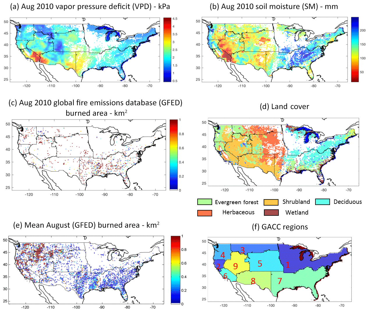
Figure 1 Snapshot of August 2010 of the datasets used in relation to the geographic area coordination centers (GACCs). Panel (e) shows the long-term mean of August GFED burned area. GACC regions are (1) Eastern, (2) Northern California (CA), (3) Northern Rockies, (4) Northwest, (5) Rocky Mountain, (6) Southern CA, (7) Southern, (8) Southwest and (9) Great Basin.

The goal of this work is to investigate the utility of remotely sensed hydrology observations for predicting fire danger, defined as the amount of area likely to burn, at spatial and temporal scales commensurate with regional and global fire management decision-making. Specifically, the objective is to investigate the utility of remotely sensed satellite-observed vapor pressure deficit (VPD) from NASA's Atmospheric Infrared Sounder (AIRS) mission and surface soil moisture (SSM) from a numerical data assimilation of terrestrial water storage from NASA's GRACE mission as indicators for predicting monthly fire danger across the United States from 2002 until 2016 at the scale of the geographic area coordination centers (GACCs; Fig. 1). To meet the objective, we test the hypothesis that burned area varies monthly as a function of previous months' water availability in the soil (SSM) and evaporative demand (i.e., previous months' VPD).

2 Methods

2.1 Datasets

For the purpose of this study, four input datasets were used (Fig. 1). First, monthly VPD (Fig. 1a) was generated from the AIRS near-surface air temperature (T_mean) and relative humidity (RH) version 6 (Aumann et al., 2003; Goldberg et al., 2003). Please refer to Behrangi et al. (2016) for the formulation based on monthly air temperature (T_mean) and dew point temperature (Td_mean) as well as the reliability of this formulation for monthly VPD derivation. The data are at a 0.5^∘ spatial resolution and have been available since September 2002. The second input to the model was monthly surface soil moisture data (Fig. 1b), produced at the NASA Goddard Space Flight Center (GSFC) using the catchment land surface model (CLSM; a physically based land surface model) and assimilated ground- and space-based meteorological observations (Houborg et al., 2012; Reager et al., 2015; Tapley et al., 2004; Zaitchik et al., 2008). The SSM data have been available since April 2004 and are at a 0.25^∘ spatial resolution. The third dataset was the Global Fire Emissions Database version 4 (GFED-4s), which provided wildfire-burned area, generated at a 0.25^∘ spatial resolution. GFED-4s is primarily derived from MODIS from 2001 to present and is reported as fraction of a cell burned for a given month (van der Werf et al., 2017). GFED data have been available since 1997. Figure 1c shows GFED burned area in August 2010, while Fig. 1e shows the long-term August burned area in square kilometers. As shown, wildfires occur all around the contiguous United States (CONUS) in August. The amount of area burned however is considerably larger in the western United States, such as in the Northern Rockies, Northwest, Rocky Mountain and Northern California GACCs. Finally, in this study, we have excluded agricultural fires by masking out agricultural regions as classified by the 2011 National Land Cover Database (Fig. 1d; Homer et al., 2015).

For consistency, all datasets were converted using linear interpolation into monthly 0.25^∘ spatial-resolution products that were then used to perform the model training and analysis for the period 2003 through 2016.

2.2 Analysis

GACCs are marked by geopolitical boundaries that also denote similar fire weather types and are used to allocate fire management resources across the contiguous United States (CONUS; Abatzoglou and Kolden, 2013; Finco et al., 2012; Fig. 1). In this study, we predict anomalous monthly burned area using a linear regression model; a separate model is developed for each GACC and for each month in a climatological sense. All fire events, for a given GACC and a month of the year, are selected as a single population for model training. For example, all fires occurring in the Northern Rockies GACC, during the months of February 2004, February 2005, February 2006, etc. through February 2016, are placed into a single population. Each monthly 0.25^∘ fire-burned area observation has a matched SSM and VPD observation at the corresponding time and grid location. These sets are then used to train the model, and various time lags are imposed between the independent variables (SSM and VPD) and the dependent variable (burned area) in order to maximize predictive skill.

Each GACC uses the best prior VPD–SSM combination for all months. The best model was identified for each GACC by selecting the model with the lagged input that represents the highest-weighted Nash–Sutcliffe efficiency (E_w):

$$\begin{array}{}\text{(1)}& E_{\mathrm{w}}={\sum }_{j=\mathrm{1}}^{\mathrm{12}}{E}_j\times {\mathrm{FAB}}_j,\end{array}$$

where FAB_j is the mean historical fraction of annual area burned in month j and E_j is the Nash–Sutcliffe (E) for any given month (j). E_j (Nash and Sutcliffe, 1970) is a metric that measures the skill of the model against the skill of the long-term mean value (i.e., persistence), defined as

$$\begin{array}{}\text{(2)}& E_j=\mathrm{1}-{\displaystyle \frac{{\sum }_{i=\mathrm{1}}^n{\left({\mathrm{AB}}_{\mathrm{obs},i}-{\mathrm{AB}}_{\mathrm{s},i}\right)}^{\mathrm{2}}}{{\sum }_{i=\mathrm{1}}^n{\left({\mathrm{AB}}_{\mathrm{obs},i}-{\mathrm{AB}}_{\mathrm{C}}\right)}^{\mathrm{2}}}},\end{array}$$

where n is total number of observations, AB_obs,i is observed area burned in month j, AB_s,i is the model-simulated area burned for month j and AB_C is the mean area burned in month j over the climatological record. E can range between −infinity and 1. An E value of zero shows that the model performance is as good as the mean of observations over the entire record. If E exceeds 0, the model performs better than the mean of observations, and if E falls below zero, the mean of observations is a better predictor than the model simulations. An E of 1 represents the perfect prediction by the model.

We constructed a forecasting method that would only rely on the model prediction of burned area, as opposed to the burned-area climatology, if the model had demonstrated skill for a given month. The estimation of E_w for each GACC and for each monthly model ensures that months with higher predictive skill are assigned a higher weight in the combined time series. Also, months exhibiting a higher amount of historical wildfire activity are assigned a higher weight.

The model is then defined as follows:

$$\begin{array}{}\text{(3)}& {\mathrm{AB}}_{\mathrm{s}}={\mathrm{AB}}_{\mathrm{C}}+{\mathrm{AB}}_{\mathrm{A}},\end{array}$$

where

$$\begin{array}{c}{\displaystyle }{\mathrm{AB}}_{\mathrm{A}}=a+b\times \left({\mathrm{VPD}}_{\mathrm{A}}\right)+c\times \left({\mathrm{SM}}_{\mathrm{A}}\right)\text{if }{E}_j>\mathrm{0}\\ {\displaystyle }{\mathrm{AB}}_{\mathrm{A}}=\mathrm{0}\text{if }{E}_j\le \mathrm{0}.\end{array}$$

AB_s is the simulated area burned for a given month; AB_c is the climatological area burned or the mean annual area burned by month; VPD_A and SSM_A are the anomalous VPD and SSM in the 1, 2 or 3 months prior to the wildfire month. Different combinations of prior VPD and SSM observations were tested to represent the reliability of a single VPD–SSM model per GACC for the entire year.

Finally, AB_S is compared to AB_C by comparing two Nash–Sutcliffe (E) values of the entire time series. The first E value is measured using the 2003–2016 monthly time series of model predictions and observations (E_{simulated,observation}). The second E value is computed by using 2003–2016 monthly time series of climatology and observations (E_{climatology,observation}). If E_{simulated,observation} exceeds E_{climatology,observation}, the model has more accuracy compared to the climatology. If E_{climatology,observation} is greater than E_{simulated,observation}, then the climatology has more accuracy in forecasting wildfire activity.

3 Results

Figure 2 shows the hydrologic-variable combination used to develop the best model of burned-area forecast using the monthly Nash–Sutcliffe coefficient (E), the weighted Nash–Sutcliffe coefficient (E_w), and the fraction of annual area burned for each month, while Table 1 shows the best variable combination for each GACC. There are some notable patterns, though few without exceptions. For example, Northern California, Northern Rockies and Northwest all have the same peak month (August) for area burned while also having significant fractions of evergreen vegetation (Fig. 1). Area burned in Great Basin also peaks in August; however it does not have substantial evergreen land cover, although at this spatial scale we can not determine if that is where fires happen. The models with the highest relative predictive ability throughout the year (denoted by weighted Nash–Sutcliffe coefficient) are generally in the GACCs with substantial land cover and dominated by fuel-limited systems (herbaceous and shrublands): Great Basin, Southern California, Rocky Mountain, Northwest and Northern Rockies; however, Southwest also has heavy herbaceous vegetation but has relatively low predictability throughout the year. To reiterate, Northern Rockies, Northwest, Rocky Mountain and Great Basin are all substantially covered by herbaceous vegetation, but they have high predictability in their peak burned-area month, unlike Southwest. One pattern that is robust is that Great Basin, Southwest, and Southern California all rely on 1-month lead-time soil moisture in their predictive model and all also have substantial shrubland cover. Notably, the Eastern, Northern Rockies, Rocky Mountain, Southern California and Southern GACCs all have bimodal burned-area distributions but no similar land cover characteristics to explain the pattern.

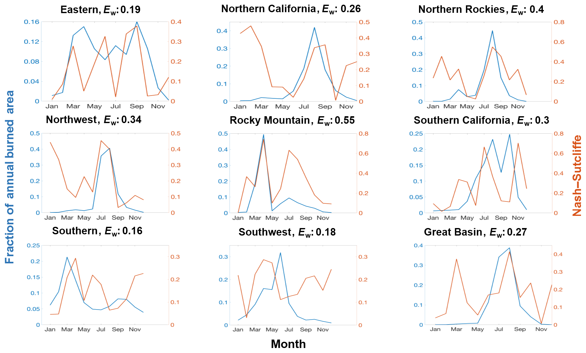
Figure 2 Best-model selection based on the monthly Nash–Sutcliffe coefficient for each GACC. The blue line shows variable peak fire month by mean annual area burned (FAB), and the orange line shows the monthly Nash–Sutcliffe coefficient for each GACC showing variable peak fire month. The weighted Nash–Sutcliffe coefficient is calculated using the different combinations of VPD and SSM. The best model was selected based on the highest E_w value, which demonstrates the relative strength of the different models by GACC.

Table 1 Overall model performance and separate influence of individual hydrologic variables. We use Nash–Sutcliffe coefficients to describe the combined surface soil moisture (SSM) and vapor pressure deficit (VPD) simulation performance (E_S), the climatology performance (E_C), and the individual predictor performance (E_S,VPD E_S,ssm) vs. the observations.

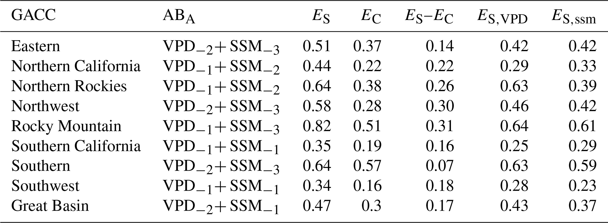
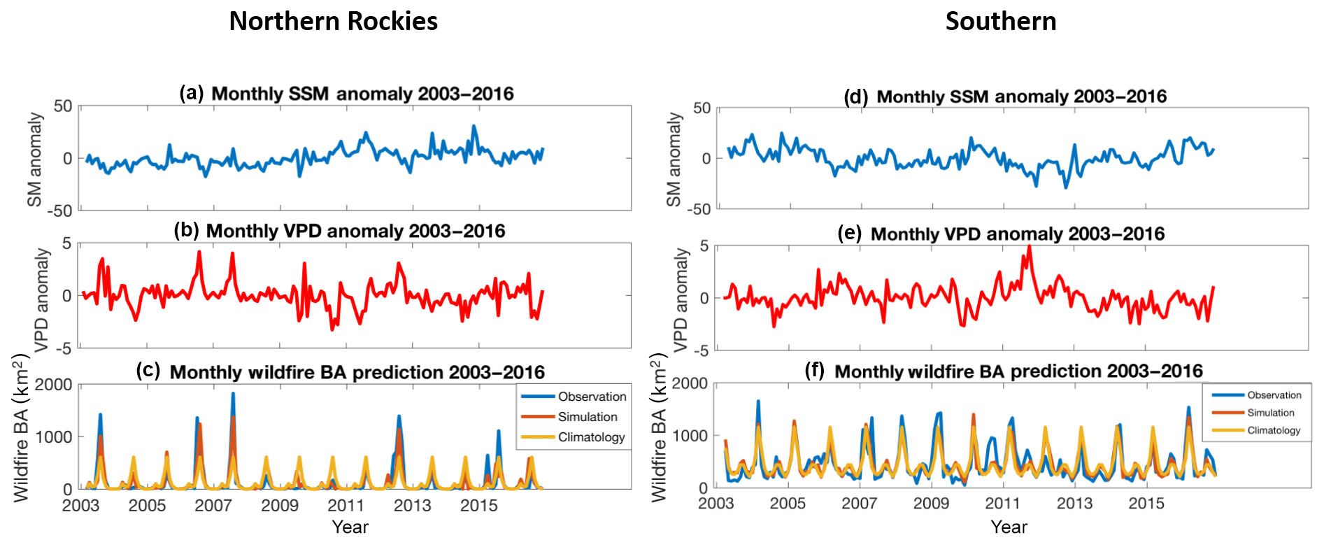
Figure 3 The impact of hydrologic predictors on best- and worst-performing Geographic Area Coordination Center (GACC) models. Monthly time series from 2003 through 2016 show the GACCs with the best (a–c) and worst (d–f) coupled response of burned area (c, f) to vapor pressure deficit anomaly (b, e) and soil moisture anomaly (a, d), thus demonstrating the respective value added by these variables in the modeled burned area (simulation in orange) compared to the climatology (yellow) and the observations (blue). BA denotes burned area.

Figure 3 shows two example cases of model predictions based on hydrological variables. We show results for our best- and worst-performing GACC in order to capture the range of model skill in different fire climate regions. For our best preforming GACC, Northern Rockies, we see consistent peaks in between the dominant hydrologic variable, VPD, and the fire area burned, suggesting the dominant role of VPD in fire-burned-area prediction for that GACC (Table 1). These strong relationships between hydrology and wildfire occurrence in Northern Rockies confirm the findings of the previous studies (Littell et al., 2009; Westerling et al., 2011). For our worst-performing GACC, Southern, two hydrologic variables are seemingly much more connected and it is less clear what drives the pattern of monthly area burned.

In order to evaluate the model predictions against the observations, we have calculated two Nash–Sutcliffe coefficients (Table 1). As shown, for all GACCs, the model forecasts the wildfire activity with higher accuracy than it does the climatology, but the improvement is variable by GACC. The results reveal that the Rocky Mountain and Northern Rockies GACCs have the best model performance (E of 0.82 and 0.64, respectively), while the Southwest and Southern CA GACCs (E of 0.34 and 0.35, respectively) show the worst model performance. Similar to the time series of the Eastern and Southern GACCs, the model has not improved the climatology to a great extent. In all other regions, the improvement of the simulated performance compared to the climatology is substantial. The key difference between the overall evaluation metric (E_S-C) and the time series is that the time series demonstrate the variability in predictive ability from month to month.

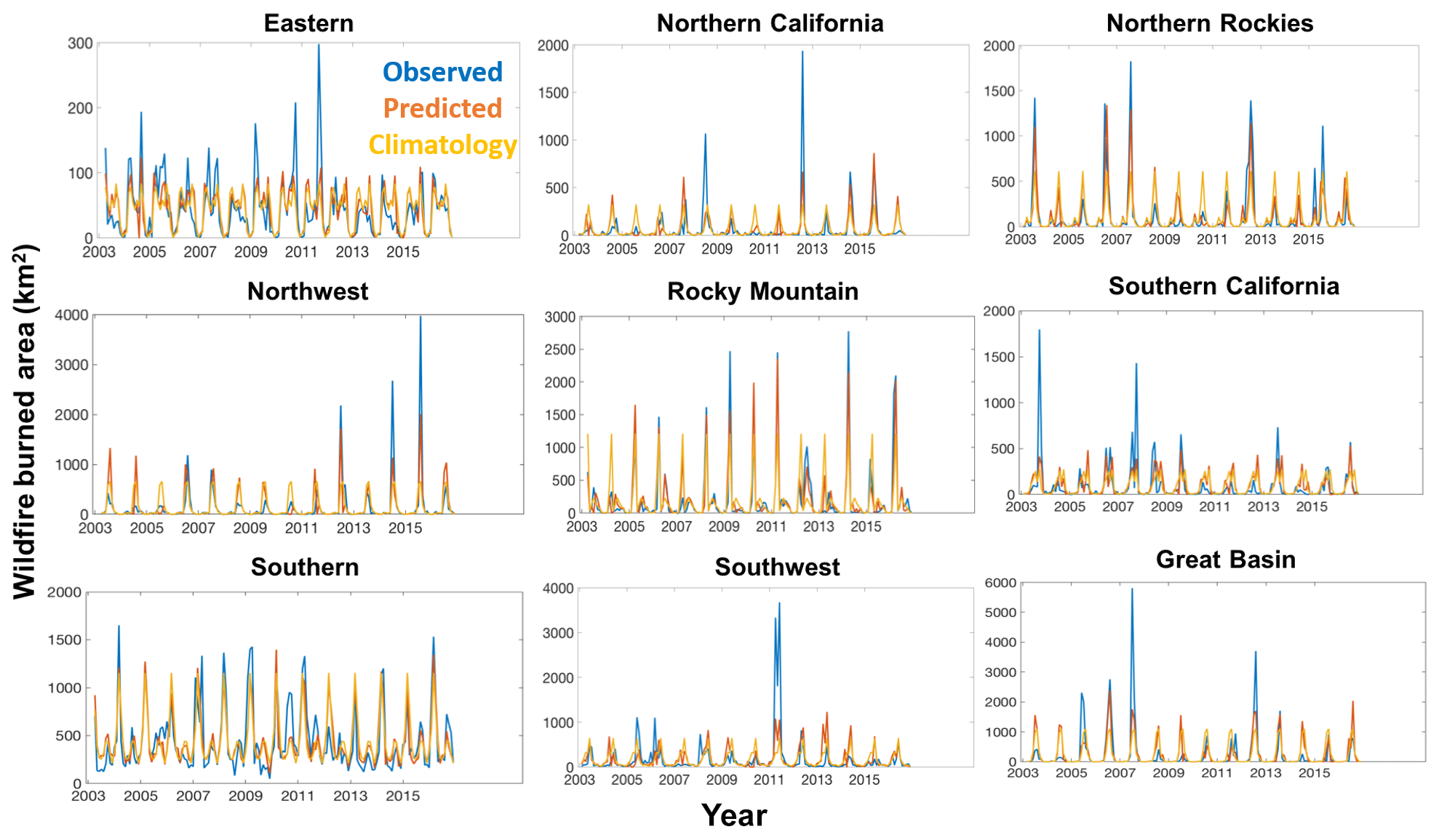
Figure 4 The ability of the regional models to predict (orange) the observed burned area (blue) is improved with the climatology (yellow), which demonstrates the ability to capture interannual variability by Geographic Area Coordination Center.

Figure 4 shows the time series of wildfire-burned-area observation (blue), simulation (red) and climatology (yellow) for nine different GACCs from 2003 through 2016. This figure shows that the performance of the models varies by location and month. In general, the models capture interannual variability for most GACCs. Notably in Fig. 4, some months show the simulation has higher agreement with the observations than the climatology does. In the southern GACCs, model performance is relatively similar to the climatology. In the Southern GACC, both the simulation and climatology indicate close agreement with the observations. Northern Rockies and Rocky Mountain show the highest agreement between model and observations in the higher-than-normal fire years. Specifically, in Northern Rockies, the model detects expected burned area for the above-normal fire activity years 2003, 2006, 2007 and 2012; and in the Rocky Mountain GACC, years 2006, 2008, 2009, 2011, 2015 and 2016 show high agreement between the simulations and the observations. The model also detects higher-than-normal fire activity in Northern California, years 2012, 2014 and 2015; Northwest, years 2006, 2007, 2012, 2014 and 2015; Great Basin, years 2006, 2007, 2012 and 2013; and Eastern for years 2004 and 2012. Lastly, the simulation outperforms the climatology slightly for Southern CA and Southwest. However, neither the model nor the climatology has detected interannual fire activity for these regions with high accuracy.

Lastly, the models were built using only either VPD or SSM to determine the relative influence of either variable on burned area within each GACC (Table 1, E_S,VPD and E_S,SSM). For some of the GACCs, the influence of the variable appears to be associated with the relative fractions of land cover influenced by that variable. For example, in Northern Rockies, it is roughly half evergreen forest and half herbaceous (Fig. 1); evergreen forest typically needs to be dry to sustain combustion (high VPD in the month prior), while herbaceous communities typically need wet conditions in the months prior to grow fuels (high SSM 2 months prior; Littell et al., 2009; Stavros et al., 2014a). Similarly, in Northwest it is roughly half evergreen (high VPD 2 months prior) and half shrub (high SSM 3 months prior). Rocky Mountain is mostly herbaceous and shrubland (high SSM 3 months prior) but has some evergreen (high VPD 1 month prior). In Northern California, land cover is mostly evergreen (high VPD 1 month prior) with some shrub (high soil moisture 2 months prior). The other GACCs have less obvious relationships between land cover and hydrology.

4 Discussion and conclusion

Wildfire activity results in billions of dollars of losses every year. Forecasting wildfire activity could therefore substantially reduce the damage associated with wildfire-burned area. Historical wildfire prediction models have limitations including the mismatch in scale between fire danger models and common application as well as the unreliability of meteorological data in remote regions. As such, current operational wildfire forecast models for forecasts >10 d are heavily based on subjective expert knowledge to predict expected area burned. Thus, the aim of this study was to predict area burned in different geographic regions (GACCs) of the United States.

There are some notable patterns in predictive-model development across GACCs largely driven by land cover fractional cover and mesoscale climate (Table 1). The Great Basin, Southwest and Southern California GACCs all have substantial shrubland cover and have the same soil moisture predictor (1-month lead time). This could be a function of the shallow rooting of shrubs. This was the only pattern by land cover that was not contradicted by mesoscale climatic influence. For example, the Great Basin, Southern California, Rocky Mountain, Northwest and Northern Rockies models have the highest predictive ability throughout the year (E_w) and have substantial land cover dominated by fuel-limited systems (grasslands and shrublands). Fuel-limited systems typically rely on pre-fire-season conditions to grow fuels that carry fire, thus influencing the total burned area (Stavros et al., 2014a; Swetnam and Betancourt, 1998). Although Southwest also has heavy grasslands, it has a relatively low predictability throughout the year but is the GACC most influenced by the southwest monsoon, which can have a variable onset that affects the fire season (Grissino Mayer and Swetnam, 2000). The southwest monsoon also explains why Northern Rockies, Northwest, Rocky Mountain and Great Basin all have high predictability in their peak burned area month, but Southwest (also substantially covered by grasslands) does not. Further substantiating the claim that mesoscale climate affects model predictability is the fact that Southern California has a bimodal distribution of fire area burned throughout the year. According to Jin et al. (2014), there are two different kinds of fire in Southern California (those in the summer driven by hot and dry conditions and those in the fall driven by Santa Ana winds), and each has different climatic conditions explaining the number of fires and burned area.

Beyond climate and land cover, humans play a significant role in the predictability of area burned (Balch et al., 2017). This explains the bimodal fire distributions found in the Eastern, Northern Rockies, Rocky Mountain and Southern GACCs. Most of the fires in the Eastern and Southern GACCs are prescribed burns, which can happen throughout the year (as denoted by the relatively flat, although slight bimodal, distributions of percent annual area burned by month – Table 1). Also, there is a notable decoupling of the relationship between hydrologic variables and burned area (Fig. 4) in the Southern GACC, which has mostly anthropogenic fire ignitions, as compared to Northern Rockies, which has mostly lightning-caused ignitions when burned area peaks in fall (Fig. 2). This also explains why the simulation performs closely to the climatology (Fig. 3), with only minor improvements in Nash–Sutcliffe coefficients as compared to other GACCs (Table 1). Notably, the GACCs that have a strong bimodal distribution perform less well than those that do not; however in all GACCs with bimodal distributions (Fig. 2), there are substantial croplands (which were excluded from the analysis) where agricultural burning occurs independent of the hydrologic conditions (Fig. 1).

Mesoscale climate (e.g., monsoons) and anthropogenic influence on fire regimes have likely less direct relationships with burned area than hydrologic variables do. Specifically, the GACCs that are more influenced by mesoscale climate (Southern California and Southwest) and by anthropogenic burning (Southern and Eastern) did not show a clear association between the relative influence of the hydrologic variable and the relative fractions of land cover, unlike Northern Rockies, Northwest, Northern California or Rocky Mountain.

In general, this work demonstrates how lead data on hydrologic variables that can be measured by satellite (i.e., not limited by proximity to in situ infrastructures) can be used to forecast fire danger 1 month before it happens. In all geographic regions, the models improved the fire danger forecast compared to the climatology (Table 1) and demonstrated the ability to capture interannual variability (Fig. 2). Future work should consider how these models are developed by land cover type and if there are different models based on how that land cover type is typically managed (e.g., cropland vs. forest).