the Creative Commons Attribution 4.0 License.
the Creative Commons Attribution 4.0 License.
 | 14 Jan 2020
Improving sub-seasonal forecast skill of meteorological drought: a weather pattern approach
Hayley J. Fowler
Christopher G. Kilsby
Robert Neal
Rutger Dankers
Dynamical model skill in forecasting extratropical precipitation is limited beyond the medium-range (around 15 d), but such models are often more skilful at predicting atmospheric variables. We explore the potential benefits of using weather pattern (WP) predictions as an intermediary step in forecasting UK precipitation and meteorological drought on sub-seasonal timescales. Mean sea-level pressure forecasts from the European Centre for Medium-Range Weather Forecasts ensemble prediction system (ECMWF-EPS) are post-processed into probabilistic WP predictions. Then we derive precipitation estimates and dichotomous drought event probabilities by sampling from the conditional distributions of precipitation given the WPs. We compare this model to the direct precipitation and drought forecasts from the ECMWF-EPS and to a baseline Markov chain WP method. A perfect-prognosis model is also tested to illustrate the potential of WPs in forecasting. Using a range of skill diagnostics, we find that the Markov model is the least skilful, while the dynamical WP model and direct precipitation forecasts have similar accuracy independent of lead time and season. However, drought forecasts are more reliable for the dynamical WP model. Forecast skill scores are generally modest (rarely above 0.4), although those for the perfect-prognosis model highlight the potential predictability of precipitation and drought using WPs, with certain situations yielding skill scores of almost 0.8 and drought event hit and false alarm rates of 70 % and 30 %, respectively.
- Article
(10039 KB) - Full-text XML
-
Supplement
(1194 KB) - BibTeX
- EndNote


Droughts are a recurrent climatic feature in the UK. Severe events, such as those in 1975–1976, 1995 and 2010–2012, had significant implications for many sectors, including agriculture, water resources and the economy, as well as for ecosystems and natural habitats (Marsh and Turton, 1996; Marsh et al., 2007; Rodda and Marsh, 2011; Kendon et al., 2013). To mitigate the effects of drought, it is crucial that relevant sectors plan ahead, and drought forecasts play an important role in designing these strategies. Despite this, there is very little published research on UK drought prediction, and studies have predominantly focussed on hydrological drought (Wedgbrow et al., 2002, 2005; Hannaford et al., 2011).
Meteorological drought is challenging to predict using dynamical ensemble prediction systems (Yoon et al., 2012; Yuan and Wood, 2013; Lavaysse et al., 2015; Dutra et al., 2013; Mwangi et al., 2014). This is primarily due to the complex processes involved in precipitation formation, making it a difficult variable to forecast beyond short lead times (Golding, 2000; Saha et al., 2014; Smith et al., 2012; Cuo et al., 2011). At longer lead times, dynamical model skill in predicting atmospheric variables tends to be much higher (Saha et al., 2014; Vitart, 2014; Scaife et al., 2014; Baker et al., 2018). This has led researchers to investigate the potential of using atmospheric forecasts as a precursor to predicting precipitation-related hazards (Baker et al., 2018; Lavers et al., 2014, 2016).
Weather pattern (WP; also called weather types, circulation patterns and circulation types) classifications are a candidate for such an application. A WP classification consists of a number of individual WPs, which are typically defined by an atmospheric variable and represent the broad-scale atmospheric circulation over a given domain (Huth et al., 2008). They can be used to make general predictions of local-scale variables such as wind speed, temperature and precipitation and are a tool for reducing atmospheric variability to a few discrete states. WP classifications have mainly been studied in the context of extreme hydro-meteorological events (Hay et al., 1991; Wilby, 1998; Bárdossy and Filiz, 2005; Richardson et al., 2018, 2019a) and as a tool for analysing historical and future changes in atmospheric circulation patterns (Hay et al., 1992; Wilby, 1994; Brigode et al., 2018). See Huth et al. (2008) for a comprehensive review of WP classifications.
Until recently, the capability of dynamical models to predict WP occurrences had been little researched. Ferranti et al. (2015) evaluated the forecast skill of the medium-range European Centre for Medium-Range Weather Forecasts ensemble prediction system (ECMWF-EPS; Buizza et al., 2007; Vitart et al., 2008) using WPs. They objectively defined four WPs according to daily 500 hPa geopotential heights over the North Atlantic–European sector. Model forecasts of this variable for October through April between 2007 and 2012 were then assigned to the closest matching WP using the root-mean-square difference. Verification scores indicated that there was superior skill for predictions initialised during negative phases of the North Atlantic Oscillation (NAO; Walker and Bliss, 1932). Similarly, WPs were used to evaluate the skill of the Antarctic Mesoscale Prediction System by Nigro et al. (2011).
To support weather forecasting in the UK in the medium to long range, the Met Office uses a WP classification, MO30, in a post-processing system named “Decider” (Neal et al., 2016). Using a range of ensemble prediction systems, forecast mean sea-level pressure (MSLP) fields over Europe and the North Atlantic Ocean are assigned to the best-matching WP according to the sum of squared differences between the forecast MSLP anomaly and WP MSLP anomaly fields. Decider therefore produces a probabilistic prediction of WP occurrences for each day in the forecast lead time. Decider has various operational applications: predicting the possibility of flow transporting volcanic ash originating in Iceland into UK airspace, highlighting potential periods of coastal flood risk around the British Isles (Neal et al., 2018), and acting as an early-forecast system for fluvial flooding (Richardson et al., 2019b).
For Japan, Vuillaume and Herath (2017) defined a set of WPs according to MSLP. These WPs were used to refine bias-correction procedures, via regression modelling, of precipitation from two global ensemble forecast systems. The authors found that improvements from the bias-correction method using WPs were strongly dependent on the WP but overall superior to the global (non-WP) method. Relevant to this study, Lavaysse et al. (2018) predicted monthly meteorological drought in Europe using a WP-based method. They aggregated ECMWF-EPS daily reforecasts of WPs to predict monthly frequency anomalies of each WP. For each 1∘ grid cell, the predictor was chosen to be the WP that corresponded to the maximum absolute temporal correlation between the monthly WP frequency-of-occurrence anomaly and the monthly standardised precipitation index (SPI; McKee et al., 1993). Using this relationship, the model predicted drought in a grid cell when 40 % of the ECMWF-EPS ensemble members forecast an SPI value below −1. Compared to direct ECMWF-EPS drought forecasts, the WP-based model was more skilful in north-eastern Europe during winter but less skilful for central and eastern Europe during spring and summer. Over the UK, the WP model appeared to be superior for north-western regions in winter but inferior in summer, although scores for the latter were of low magnitude.
The aforementioned studies have all considered daily WPs. An example of WPs defined on the seasonal timescale was presented by Baker et al. (2018). The authors analysed reforecasts of UK regional winter precipitation between the winters of 1992–1993 and 2011–2012 using GloSea5, which has little raw skill in forecasting this variable (MacLachlan et al., 2015). GloSea5 has, however, been shown to skilfully forecast the winter NAO (Scaife et al., 2014). Baker et al. (2018) exploited this by constructing two winter MSLP indices over Europe and the North Atlantic, and reforecasts of these indices were derived from the raw MSLP fields. A simple regression model then related these indices to regional precipitation and produced more skilful forecasts than the raw model output.
In this study, we explore the potential for utilising a WP classification (specifically MO30) in UK meteorological drought prediction. We predict WPs using two models, the ECMWF-EPS and a Markov chain, from which precipitation and drought forecasts are derived. These models will be compared to direct precipitation and drought forecasts from ECMWF-EPS. We also run an idealised, perfect-prognosis model that uses WP observations rather than forecasts as an “upper benchmark” to assess the upper limit of the usefulness of the WP classification. Section 2 contains details of the data sets used, including describing the creation of a WP reforecast data set. Section 3 describes the models in detail and the forecast verification procedure. In Sect. 4, we present the results, and in Sect. 5, we draw some conclusions and make recommendations for future work.
We use a Met Office WP classification called MO30 (Neal et al., 2016). WPs in MO30 were defined by using simulated annealing to cluster 154 years (1850–2003) of daily MSLP anomaly fields into 30 distinct states. The data were extracted from the European and North Atlantic daily to multidecadal climate variability (EMULATE) data set (Ansell et al., 2006) in the domain 35–70∘ N, 30∘ W–20∘ E, with a spatial resolution of 5∘ latitude and longitude. These 30 WPs are therefore representative of the 30 most common patterns of daily atmospheric circulation over Europe and the North Atlantic (Fig. 1), and they were ordered such that WP1 is the most frequently occurring WP annually, while WP30 is the least frequent. A consequence of the clustering process and ordering is that the lower-numbered WPs have lower-magnitude MSLP anomalies and are more common in the summer than in the winter and vice versa for the higher-numbered WPs (Neal et al., 2016; Richardson et al., 2018).
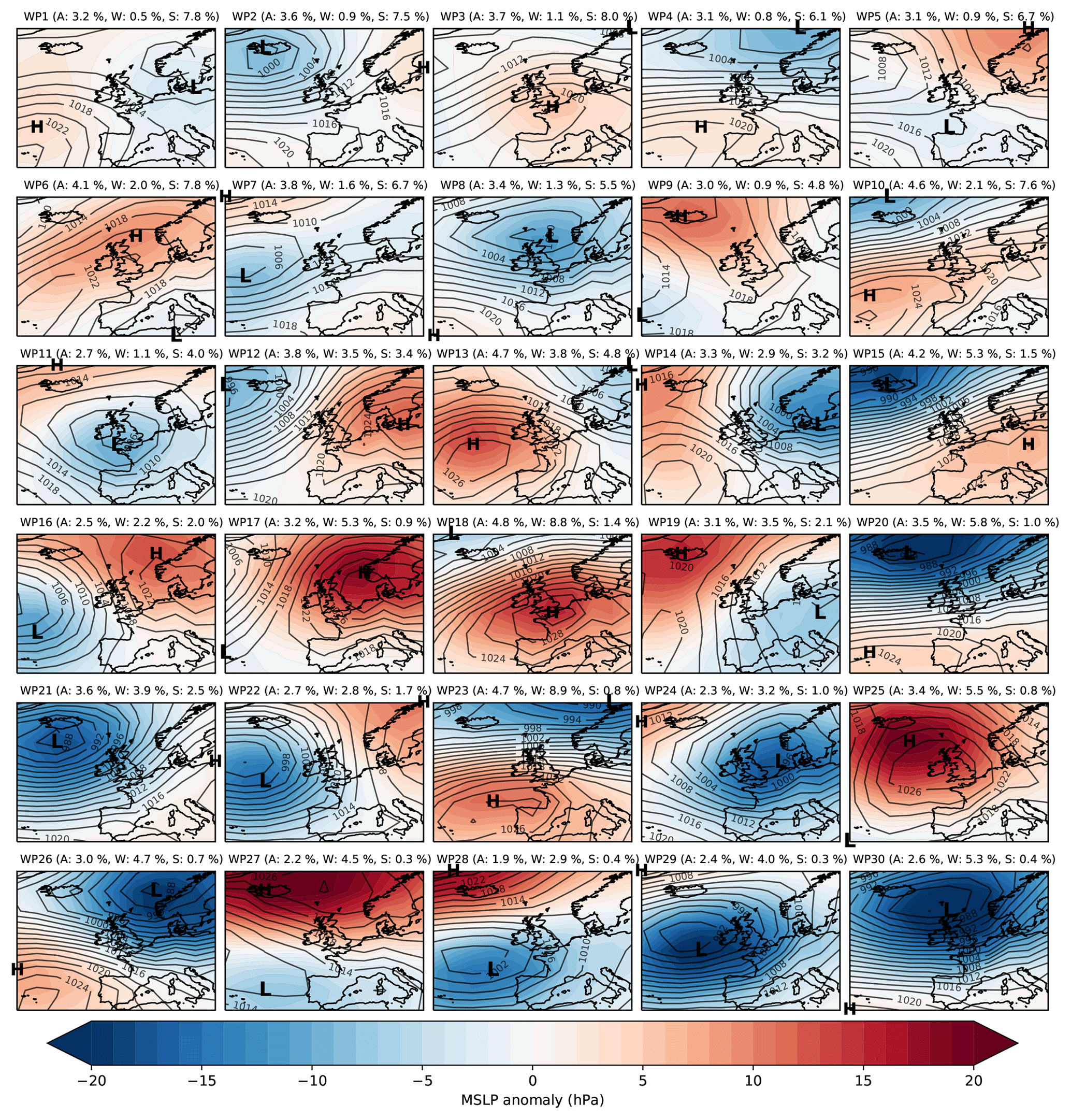
Figure 1Weather pattern (WP) definitions according to mean sea-level pressure (MSLP) anomalies (hPa). The black contours are isobars showing the absolute MSLP values associated with each weather pattern, with the centres of high and low pressure also indicated. Next to the WP labels are the annual (A), winter (W; DJF) and summer (S; JJA) relative frequencies of occurrences of each WP (%). The frequency-of-occurrence data are associated with the WPs based on ERA-Interim between 1979 and 2017, while the WP definitions were generated from a clustering process applied to EMULATE MSLP reanalysis data between 1850 and 2003. See the text for details.
For this analysis, we have created a 20-year daily WP probabilistic reforecast data set. We use the sub-seasonal to seasonal (S2S) project (Vitart et al., 2017) data archive, which, through ECMWF, hosts reforecast data for a multitude of variables and by a range of models from around the globe. In particular, we use ECMWF-EPS, which is a coupled atmosphere–ocean–sea–ice model with a lead time of 46 d. The horizontal atmospheric resolution is roughly 16 km up to day 15 and 32 km beyond this. The model is run at 00:00 Z twice weekly (Mondays and Thursdays) and has 11 ensemble members for the reforecasts (compared to 51 members for the real-time forecasts). For further details, refer to the model web page (ECMWF, 2017). We use daily reforecasts of MSLP between 2 January 1997 and 28 December 2016, inclusively, with the same domain and resolution as MO30. These fields are converted to forecast anomalies by removing a smoothed climatology and subsequently assigned to the closest matching MO30 WP via minimising the sum-of-squared differences. Both the MSLP climatology and the WP definitions are the same as those used by Neal et al. (2016) to ensure consistency. We compare this against an “observed” WP time series to measure forecast skill. For this, WPs are assigned from 00:00 Z MSLP fields from the ERA-Interim reanalysis data set (Dee et al., 2011) between 1979 and 2017. A consequence of assigning WPs using ERA-Interim compared to the EMULATE data set used in the original derivation of MO30 is that the historical frequencies of occurrence of the WPs differ. The same strongly seasonal behaviour is retained (lower-numbered WPs occurring more often in summer than higher-numbered WPs and vice versa), but the annual frequencies are more evenly distributed across the WPs – there is no clear decrease in annual frequency as the WP number is increased (Fig. 1).
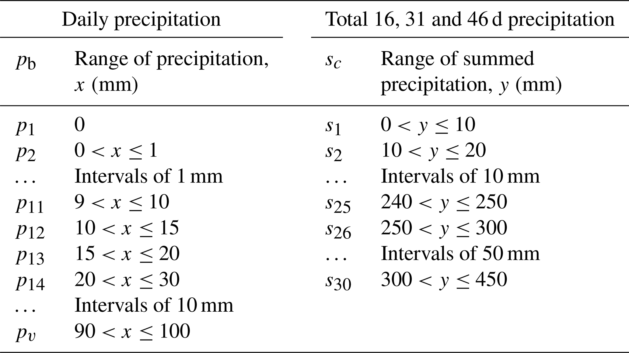
As observed precipitation, we use the Met Office Hadley Centre UK precipitation (HadUKP) data set (Alexander and Jones, 2000). HadUKP consists of nine regions covering the UK: northeastern England (NEE), central and eastern England (CEE), southeastern England (SEE), southwestern England and southern Wales (SWE), northwestern England and northern Wales (NWE), eastern Scotland (ES), northern Scotland (NS), southwestern Scotland (SS) and Northern Ireland (NI). Using daily precipitation series from 1979 to 2017, we discretise the data into precipitation intervals (“bins”) defined in Table 1; see Sect. 3.2 for further information. The large region sizes in HadUKP are suitable both for analyses of drought, which is typically considered a regional rather than localised event (Marsh et al., 2007), and for MO30 because they correspond to the large-scale circulation patterns that the WPs represent. From the S2S archive, we extract ECMWF-EPS precipitation reforecasts for the same dates as the WP reforecast data set. The data have a resolution of 0.5∘ latitude and longitude; grid cells are assigned to whichever of the nine HadUKP regions the cell centres lie in (Fig. S1 in the Supplement), and by taking the daily mean of all cells over each region, we produce a probabilistic reforecast data set of precipitation for each of the HadUKP regions. Then, we remove the 3-monthly-mean bias of the forecasts compared to the observations for each region. The bias correction is done using leave-one-year-out cross validation. Finally, these data are discretised in the same way as the HadUKP data.
Table 1Range of daily precipitation, x, for each bin pb and of 16, 31 and 46 d total precipitation, y, for each bin sc.
3.1 Weather pattern forecast models and verification procedure
For WP forecasts, we compare two models. The first is ECMWF-EPS, which we refer to as EPS-WP (in practice this is the WP reforecast data set discussed in the previous subsection). The second model is a 1000-member, first-order, nonhomogeneous Markov chain, with separate transition matrices for each month. This is similar to the Markov model used for a simulation study by Richardson et al. (2019a), who found that it was able to reasonably replicate the observed frequencies of occurrences of the MO30 WPs. Full details of the Markov model are given in the Supplement.
To evaluate WP forecast skill we use the Jensen–Shannon divergence (JSD), suitable for measuring the distance between two probability distributions (Lin, 1991). It is based on information entropy, which is used to measure uncertainty. An information-theoretic approach to verification is not widespread, although there is some published research on the topic (Leung and North, 1990; Kleeman, 2002; Roulston and Smith, 2002; Ahrens and Walser, 2008; Weijs et al., 2010; Weijs and v. d. Giesen, 2011). The JSD will be used to measure the forecast performance by quantifying the distance between distributions of the observed and forecast WP frequencies. The JSD is based on the Kullback–Leibler divergence (KLD; Kullback and Leibler, 1951). Let P and Q be two discrete probability distributions. The KLD from Q to P is given by
measured in bits (i.e. a binary unit of information). In our application I=30, the number of WPs and , …, pf,30) and , …, qf,30) are the vectors of observed and forecast WP relative frequencies, respectively. (Because these are relative frequencies, and .) As there would inevitably be some cases where the model predicts no occurrences of some WPs (i.e. when Q contains zeros), DKL(P||Q) will be undefined at times. Using the JSD avoids this problem; it is defined as
where . Unlike the KLD, the JSD is symmetric, i.e. DJSD(P||Q)≡DJSD(Q||P). Also, , with a score of zero indicating that P and Q are the same (a perfect forecast). Equation (2) gives the JSD for a single forecast–event pair; to obtain the average JSD for all forecasts, we take the mean of all forecast–event pairs. Skill is evaluated separately for each month, with the middle date of each forecast period used to assign the month. We calculate forecast skill for lead times of 16, 31 and 46 d. We use the JSD to compare WP forecast skill of EPS-WP and the Markov model, considering each lead time separately.
3.2 Precipitation and drought forecast models
We compare four models, three of which are forecast models while one model is a perfect-prognosis model. Figure 2 shows a schematic of the procedure involved in generating forecasts from each model. All models are considered at the same lead times to be the WP predictions. Two of the forecast models are driven first by a WP component: EPS-WP and the Markov model described above. The perfect-prognosis model, Perfect-WP, is used as an “upper benchmark” with (future) observed WPs as input rather than forecast WPs. It is an idealised model that cannot be used operationally, but it allows us to assess the potential usefulness of WPs in precipitation and drought forecasting. Note that from here, any reference to drought refers specifically to meteorological drought.
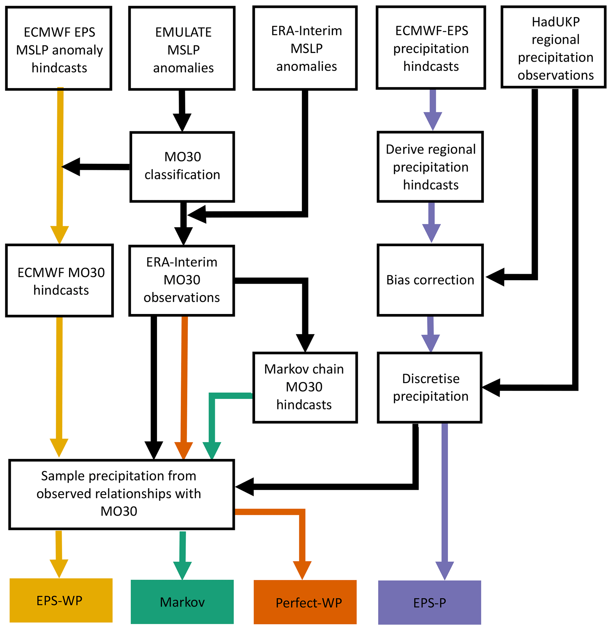
Figure 2Schematic showing the procedure for the four precipitation forecast models. The top row shows the base data sets used, and the bottom row shows the four models. Coloured arrows begin at the first stage for which forecasts are issued: EPS-WP forecasts begin with the ECMWF prediction system MSLP forecasts, Markov forecasts are produced once the ERA-Interim MO30 time series has been derived, and Perfect-WP “forecasts” are observations from the same time series, while EPS-P forecasts are the post-processed data from the ECMWF forecast system.
Precipitation is estimated from the WP predictions (or observations in the case of Perfect-WP) by sampling from the conditional distributions of precipitation given each Era-Interim WP between 1979 and 2017. We process the daily HadUKP precipitation data by discretising into v bins with historical probabilities pb for b=1, …, v. Dry days form one bin, and bin intervals increase for higher precipitation values (Table 1). This gives a discrete distribution of precipitation interval relative frequencies, D(z), with conditional distributions for each WP given by D(z|W=i), for i=1, …, 30. We also define w summed precipitation intervals sc for c=1, …, w. Forecast probabilities of these summed intervals are derived from the WP forecast models as follows.
-
Set the ensemble member …, , where Ne is the number of ensemble members, and time to t=0, the first day of the forecast. Then the predicted WP by ensemble member e at time t is We(t)=i for i=1, …, 30.
-
Set p0=0 and calculate the probabilities p1, … pm of each of the m daily precipitation bins from the discrete precipitation distribution that is conditional on We(t) and on the 91 d windows centred on t (i.e. t−45, …, t+45) from every year except the current year. This last condition is equivalent to a leave-one-year-out cross-validation procedure.
-
Define the maximum value of each bin as , b=1, …, v, with . Note that , ensuring that zero precipitation days can be simulated.
-
Generate u random variables (0, 1) for k=1, …, u.
-
For each , find the index q such that . Set and , the cumulative probabilities of the bins adjacent to .
-
Define the difference between the adjacent bins as and the difference between the random number and the lower cumulative probability as .
-
Estimate the precipitation value for each as . We now have u predicted daily precipitation values at time t, r(t)=(r1(t), …, rn(t)).
-
Set and repeat steps 3 to 6 until the final day of the forecast, tmax, is processed.
-
Sum the daily precipitation vectors and divide by the random sample size for τ=0, …, tmax.
-
Discretise according to the w summed precipitation bins s1, …, sw to obtain a distribution of relative frequencies for this ensemble member , …, fe,w).
-
Set a new ensemble member , …, , with and repeat steps 2 to 10 until every ensemble member has been processed.
-
Sum each ensemble member's distribution of summed precipitation relative frequencies (element-wise) and divide by the number of ensemble members to obtain a final forecast probability distribution: .
The number of ensemble members depends on the model. For EPS-WP, Ne=11, i.e. the number of ensemble members of the ECMWF dynamical model. For the Markov model Ne=1000. We set the number of samples drawn from each WP-precipitation conditional distribution as u=10 000. The fourth model (the third forecast model) is the direct ECMWF-EPS precipitation forecasts (EPS-P), processed to provide probabilistic predictions of regional precipitation intervals as described earlier.
3.3 Precipitation forecast verification
To evaluate precipitation forecast performance, we use the ranked probability score (RPS; Epstein, 1969; Murphy, 1971). We express the RPS as the ranked probability skill score (RPSS) using
where RPSref is the score of a climatological forecast, which in our case is the climatological event category (i.e. precipitation interval) relative frequencies (PC). A perfect score is achieved when RPSS = 1, which is also the upper limit. Negative (positive) values indicate that the forecast is performing worse (better) than RPSref.
3.4 Drought forecast verification
We evaluate model performance in predicting dichotomous drought or non-drought events. We define two classes of drought severity. The first class, mild drought, is when precipitation sums (over the length of the considered lead time: either 16, 31 or 46 d) are below the 30.9th percentile of the summed precipitation distribution. The second class is moderate drought, with such sums being below the 15.9th percentile. These percentiles are calculated for each region and month using the whole data set from 1979 to 2017 and are chosen as they correspond to SPI values of −0.5 and −1, respectively.
3.4.1 The Brier skill score
We use three verification techniques to assess skill in predicting droughts. The first is the Brier skill score (BSS). The BSS is based on the Brier score (BS; Brier, 1950), which measures the mean-square error of probability forecasts for a dichotomous event, in this case the occurrence or non-occurrence of drought. The BS is converted to a relative measure, or skill score, by setting
where BSref is the score of a reference forecast given by the quantiles associated with each drought threshold, 0.309 for mild drought and 0.159 for moderate drought. As with the RPSS, a perfect score is achieved when BSS = 1 and negative (positive) values indicate that the forecast is performing worse (better) than BSref.
3.4.2 Reliability diagrams – forecast reliability, resolution and sharpness
The BS can be decomposed into reliability, resolution and uncertainty terms (Murphy, 1973):
enabling a more in-depth assessment of forecast model performance. Reliability diagrams offer a convenient way of visualising the first two of these terms (Wilks, 2011). These diagrams consist of two parts, which together show the full joint distribution of forecasts and observations. The first element is the calibration function, g(o1|pi) for i=1, …, n, where o1 indicates the event (here, a drought) occurring, and the pi values are the forecast probabilities. The calibration function is visualised by plotting the event relative frequencies against the forecast probabilities and indicates how well calibrated the forecasts are. We split the forecast probabilities into 10 bins (subsamples) of 10 % probability, and the mean of all forecast probabilities in each bin is the value plotted on the diagrams (Bröcker and Smith, 2007). Points along the 1:1 line represent a well-calibrated, reliable, forecast, as event probabilities are equal to the forecast probabilities and suggest that we can interpret our forecasts at “face value”. If the points are to the right (left) of the diagonal, the model is over-forecasting (under-forecasting) the number of drought events.
The forecast resolution can also be deduced from the calibration function. For a forecast with poor resolution, the event relative frequencies g(o1|pi) only weakly depend on the forecast probabilities. This is reflected by a smaller difference between the calibration function and the horizontal line of the climatological event frequencies and suggests that the forecast is unable to resolve when a drought is more or less likely to occur than the climatological probability. Good resolution, on the other hand, means that the forecasts are able to distinguish different subsets of forecast occasions for which the subsequent event outcomes are different to each other.
The second element of reliability diagrams is the refinement distribution, g(pi). This expresses how confident the forecast models are by counting the number of times a forecast is issued in each probability bin. This feature is also called sharpness. A low-sharpness model would overwhelmingly predict drought at the climatological frequency, while a high-sharpness model would forecast drought at extreme high and low probabilities, reflecting its level of certainty with which a drought will or will not occur, independent of whether a drought actually does subsequently occur or not.
3.4.3 Relative operating characteristics
As a final diagnostic, we use the relative operating characteristic (ROC) curve (Mason, 1982; Wilks, 2011), which visualises a model's ability to discriminate between events and non-events. Conditioned on the observations, the ROC curve may be considered a measure of potential usefulness – it essentially asks what the forecast is given that a drought has occurred. The ROC curve plots the hit rate (when the model forecasts a drought and a drought subsequently occurs) against the false alarm rate (when the model forecasts a drought but a drought does not then occur). We compute the hit rate and false alarm rate for cumulative probabilities between 0 % and 100 % at intervals of 10 %. A skilful forecast model will have a hit rate greater than a false alarm rate, and the ROC curve would therefore bow towards the top-left corner of the plot. The ROC curve of a forecast system with no skill would lie along the diagonal, as the hit rate and false alarm rate would be equal, meaning that the forecast is no better than a random guess. The area under the ROC curve (AUC) is a useful scalar summary. The AUC ranges between zero and 1, with higher scores indicating greater skill.

To reduce information overload, we do not show results for every combination of region, lead time and drought class. Key results not shown will be conveyed via the text. We aggregate the precipitation results from monthly to 3-month seasons for visual clarity and combine regional results for the ROC and reliability diagrams for the same reason.
4.1 WP forecasts
We find that EPS-WP is more skilful at predicting the WPs than the Markov model for every month and every lead time, although the difference in skill between the two models decreases as the lead time increases. The skill difference between models is much larger for a lead time of 16 d compared to a lead time of 46 d (Fig. 3). For a 46 d lead time, the difference in skill is negligible for May through October; in fact, these months have the smallest differences in JSD for all lead times. This is presumably because the summer months are associated with fewer WPs compared to winter (Richardson et al., 2018), resulting in a more skilful Markov model due to higher transition probabilities.
An interesting result is how JSD scores for Markov decrease as the lead time increases (Fig. 3), suggesting an improvement in skill with lead time. This is the opposite of the expected (and usual) effect. The Markov model predicts WPs using the 1 d transition probabilities, and its ensemble members therefore diverge very quickly, resulting in a distribution of predicted WPs that looks similar to the climatological WP distribution for all lead times. For a 16 d forecast, the observed WP distribution of the corresponding 16 d will generally be less similar to the climatological WP distribution than for 31 d forecasts and less similar still than for 46 d forecasts. For instance, at a 16 d lead, only 16 unique WPs could form the observed distribution, whereas Markov is capable of predicting all possible WPs across its 1000 members at this lead. As the JSD measures the distance between these probability distributions, it tends to score the differences between these distributions as more similar (a smaller divergence) for longer lead times. This means that the JSD is perhaps not appropriate as a verification metric in an operational sense but is noteworthy for highlighting the behaviour of the Markov model.
We could have assessed model skill in predicting the WPs using more common metrics such as the BS, which could measure the hit ∕ miss ratio for each WP at each lead time. However, the focus of this paper is on multi-week precipitation (and drought) totals, so we are not particularly interested in the models' ability to predict the timing of a WP, only whether they are able to capture the distribution of the WP frequencies of occurrence. It is likely that using the BS would show that EPS-WP and Markov skill decreases with lead time, as was the case for a WP classification derived from MO30 by Neal et al. (2016).
4.2 Precipitation forecasts
We first discuss the skill of the three true forecast models, EPS-WP, EPS-P and Markov. For the most part, all three models are more skilful than climatology independent of season and lead time, with greater skill in autumn and winter compared to spring and summer (Figs. 4 and 5). For a 16 d lead time, there is little to choose between EPS-WP and EPS-P, except in ES, for which the latter model is less skilful than climatology in winter and spring (Fig. 4). Markov is the least skilful model at this lead, offering only a marginal improvement on climatology (Fig. 4). The skill of EPS-WP and EPS-P reduces when a 31 d lead is considered, bringing their skill more into line with Markov (Fig. S2). At a 46 d lead the differences are starker, with EPS-P being notably less skilful than EPS-WP, Markov and climatology for many regions in summer and, especially, spring (Fig. 5). These results are, however, still only marginally superior to climatology. EPS-WP has greater skill than EPS-P at this lead time in winter and autumn for NS, NI, CEE and SWE, although the magnitudes of these differences are small (Fig. 5). There is little evidence of coherent regional variability in model skill, except perhaps a tendency for EPS-P to score more highly for western regions in spring and summer at a 16 d lead time (Fig. 4). Despite low skill relative to climatology at longer lead times, there is clearly some benefit to using the WP-based models (particularly EPS-WP) for certain regions and seasons.
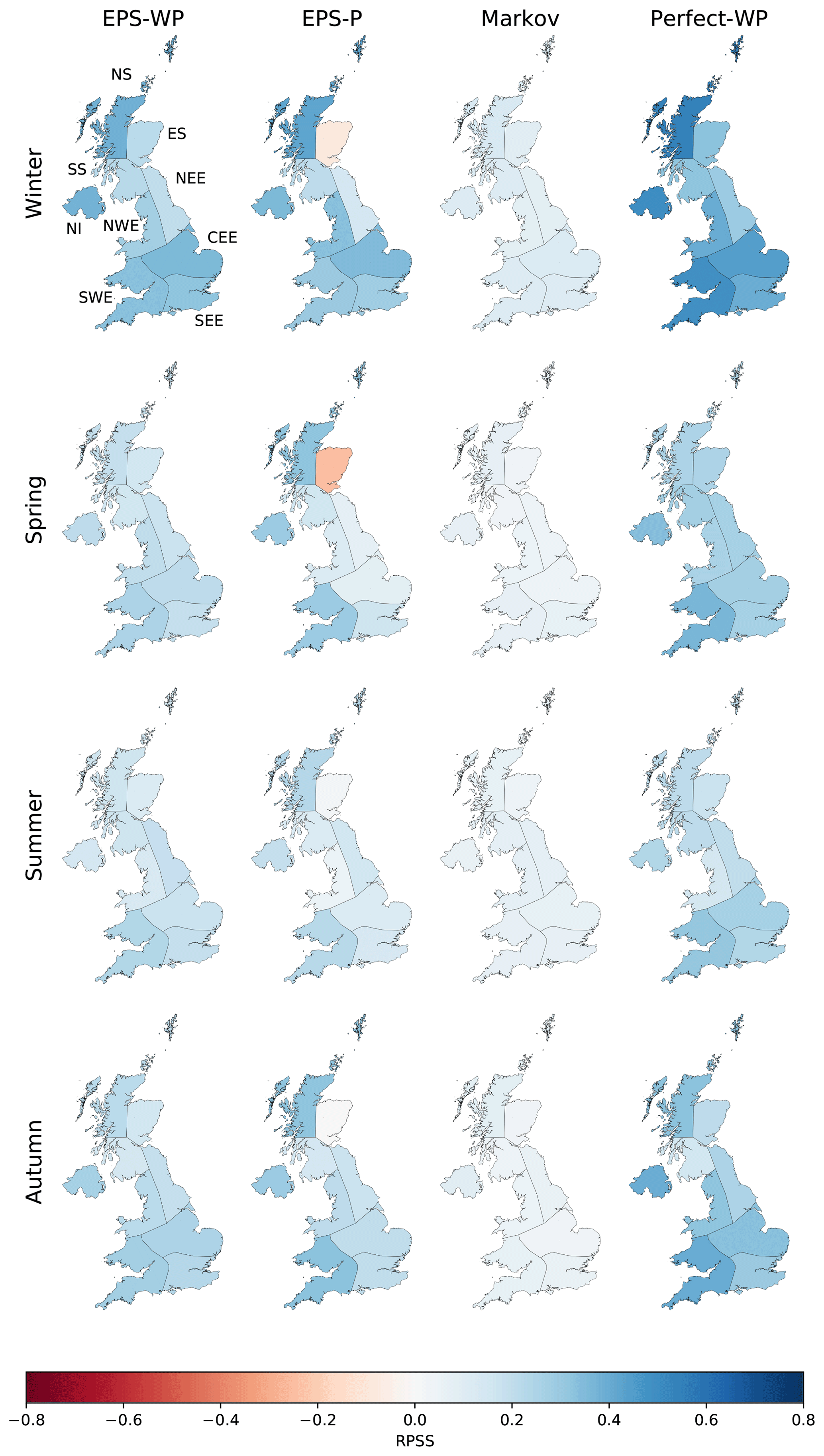
Figure 4The ranked probability skill score (RPSS) for precipitation forecasts at a 16 d lead for each model and season.
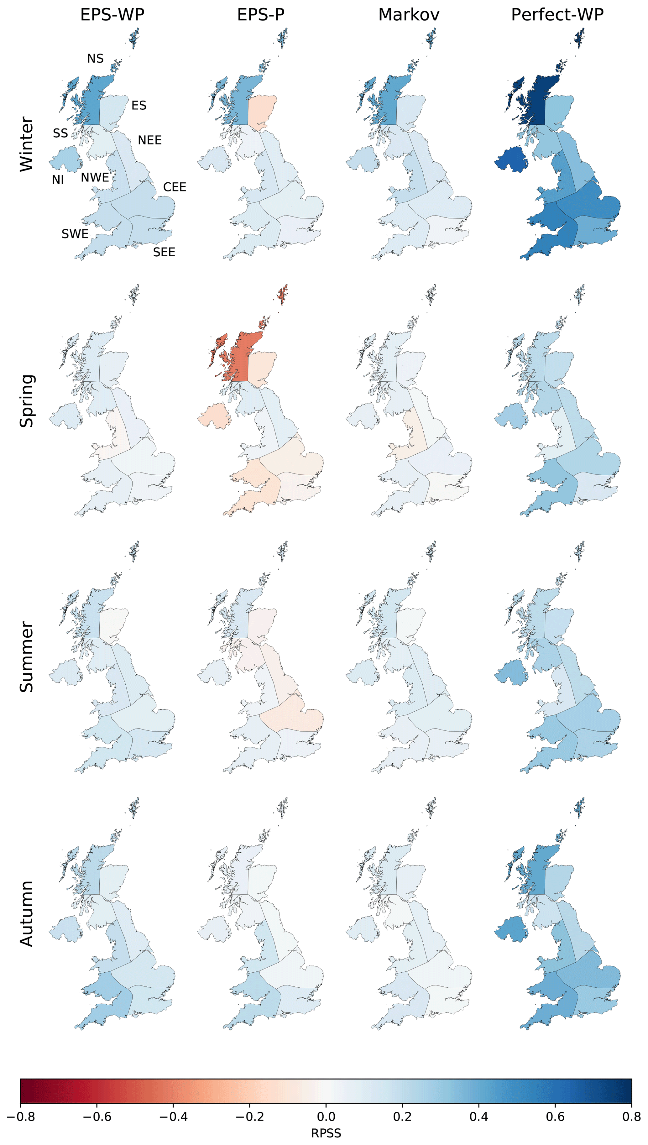
Figure 5As Fig. 4 but for a 46 d lead.
The potential usefulness of such approaches is highlighted by the performance of Perfect-WP. Unsurprisingly, this model is almost uniformly the most skilful model for all regions, seasons and lead times (Figs. 4, 5 and S2). The gains in skill for this model over the other three models are most pronounced during winter and autumn and especially for longer lead times. Skill is greatest for most western regions (NS, NI, NWE and SWE) and lowest for eastern regions ES, NEE and SEE, together with SS (Fig. 5). Perfect-WP is obviously not practical, but the results serve to show that WPs are a potentially useful tool in medium-range precipitation forecasting.
4.3 Meteorological drought forecasts
4.3.1 Forecast accuracy
Forecast accuracy is typically lower for mild drought (total precipitation over 16, 31, or 46 d below the 30.9th percentile) than for precipitation and lower still for moderate drought (total precipitation below the 15.9th percentile). The regional and lead-time differences in precipitation skill are also evident for drought, with higher skill at shorter leads and during winter and autumn (Figs. 6, 7 and S3). Results for mild drought are not shown, as they generally lie in between those for precipitation (Figs. 4, 5 and S2) and moderate drought (Figs. 6, 7 and S3). Markov again has the poorest skill, with a climatology forecast preferable for many combinations of region and lead time. EPS-P is either equal to or more skilful than EPS-WP at a 16 d lead (Fig. 6) and during spring for longer leads (Figs. 7 and S3). Conversely, EPS-WP outperforms EPS-P during summer at the longer two lead times, although a climatology forecast would be just as, if not more, skilful. As with precipitation forecasts, any gain in skill using EPS-WP over EPS-P in winter and autumn at longer leads is marginal, with both models showing more skill than climatology (Figs. 7 and S3).
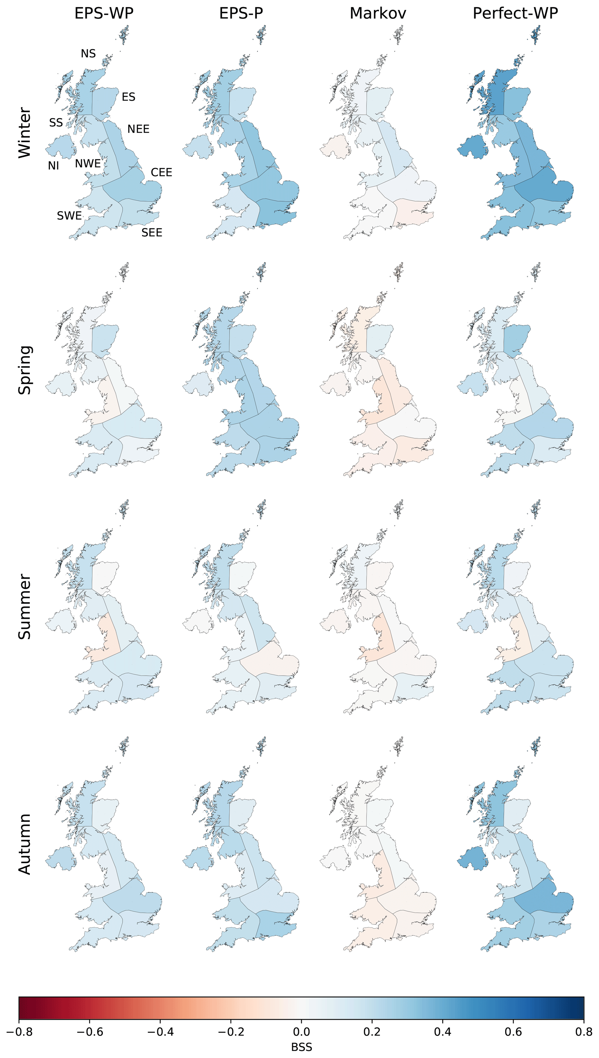
Figure 6The Brier skill score (BSS) for mild drought (total precipitation below the 30.9th percentile) for a 16 d lead time for each model and season.
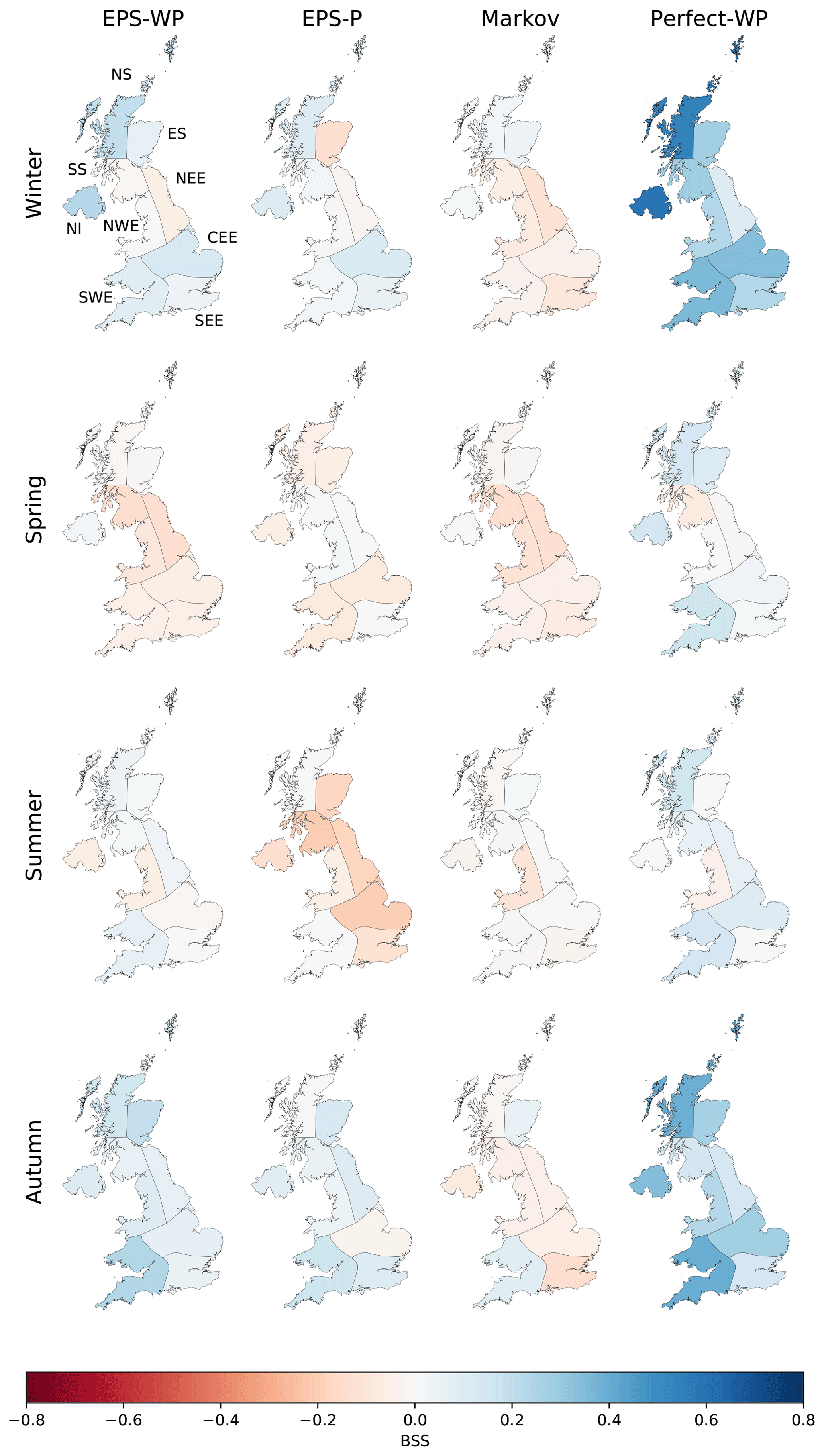
Figure 7As Fig. 6 but for a 46 d lead.
Skill, where present, is undeniably modest, but the relatively high skill of Perfect-WP in some regions and seasons again shows the potential predictability of drought using WP methods. Compared to precipitation forecasts, skill for Perfect-WP is notably lower for spring and summer, with climatology often being a competitive forecast method at a 46 d lead time (Fig. 7). For winter and autumn, however, the skill is reasonable UK-wide and particularly high during winter in NS and NI (Fig. 7). The same east–west skill split is present for moderate drought as it was for precipitation, with some western regions benefitting from higher skill than eastern regions (Fig. 7).

Figure 8Relative operating characteristic (ROC) curves and area under ROC curve (AUC) for mild drought with a 46 d lead time. Annotated values indicate drought forecast probability thresholds.
4.3.2 Relative operating characteristics
All models are better able to discriminate between drought and non-drought events than random chance, with Perfect-WP being the most able and Markov the least able, subject to similar caveats regarding lead time and season as for the BSS and RPSS results. During summer and spring, EPS-P has the highest AUC of any of the three forecast models (Figs. 8 and 9) and for a 16 d lead-time scores similarly to Perfect-WP (not shown). On the other hand, EPS-WP is the best discriminator during winter and autumn at a 46 d lead time, although the magnitude of the differences is small (Figs. 8 and 9). Markov is consistently the least suitable model for predicting drought according to the ROC curve, although it still represents a better method of doing so than random chance.
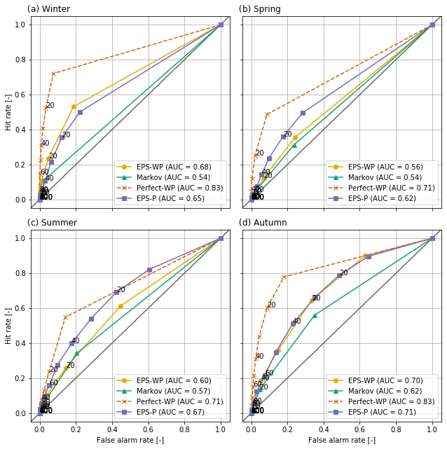
A use of the ROC curve is to provide end users with information on how to apply the considered forecast models. As the plotted points on each curve indicate the hit rate and false alarm rate associated with predicting droughts at each probability interval, they can be used to make an informed decision in selecting a probability threshold for issuing a drought forecast. For example, should a forecaster choose to issue a moderate drought warning in winter at a 10 % probability level and 46 d lead time (Fig. 9), then they would expect EPS-WP to achieve a hit rate over double that of the false alarm rate (∼55 % and ∼20 %, respectively). EPS-P, meanwhile, shows a slightly lower hit rate and similar false alarm rate (∼50 % and ∼20 %). The idealised benchmark model (Perfect-WP) achieves an outstanding score – an over 70 % hit rate compared to a less than 10 % false alarm rate. For mild drought, a 20 % probability threshold for EPS-WP and EPS-P achieves at least 60 % hit rates at all lead times, whereas for moderate drought, this threshold will only achieve such hit rates at a 16 d lead time during winter and autumn (EPS-P also achieves this rate for spring and summer; not shown) and during autumn for all lead times. In general, it appears that these low probability thresholds yield the best compromise between hits and false alarms, although in practice, the costs (e.g. financial) associated with false alarms and missed events will determine how responders use these probabilities.
4.3.3 Forecast reliability, resolution and sharpness
EPS-WP is the most reliable forecast model (i.e. excluding Perfect-WP), and while all three WP-driven forecast models tend to under-forecast droughts, EPS-P only does so for lower probability thresholds, with the higher thresholds resulting in this model over-forecasting. This is particularly true for shorter lead times and during winter, although it is still clear for 31 d lead times in some seasons (Figs. 10 and 11). Sometimes EPS-WP follows the same pattern as EPS-P and over-forecasts drought occurrence for higher predicted probabilities (e.g. Figs. 10c, e and g and 11c). However, the total number of forecasts issued in these intervals is generally smaller than for EPS-P, as the refinement distributions show most clearly for mild drought (Fig. 10). This means that the corresponding points of the calibration function are less reliable for EPS-WP (and Markov) due to smaller sample sizes (Bröcker and Smith, 2007). In fact, all three WP-based models have occasions when there are no issued forecasts with certain probabilities. These are high probabilities for Perfect-WP and EPS-WP (Fig. 11c and e) but can be as low as between 30 % and 40 % for Markov (Fig. 11e and g). As such, although EPS-WP appears to be the most reliable model from looking only at the calibration function, there is less certainty of this fact for moderate drought and for higher forecast probabilities. This erratic behaviour of the conditional event relative frequencies is most obvious in Fig. 11c and is explained by the very low sample sizes of forecasts issued with anything but a small probability (Fig. 11e; Wilks, 1995). An interesting result is that forecasts from EPS-WP are more reliable than from Perfect-WP when the predicted drought probabilities are below 80 % for mild drought (Fig. 10) and 60 % for moderate drought (except in spring; Fig. 11), despite having lower accuracy (e.g. Fig. 6). As a more skilful BSS is composed of smaller reliability and larger resolution terms (Kharin and Zwiers, 2003), it follows that the resolution of Perfect-WP is sufficiently large to overcome the larger reliability term compared to EPS-WP and yield an overall more accurate forecast model. However, for drought forecasts issued with higher probabilities, EPS-WP is the less reliable model, under- or over-forecasting drought (depending on the season) more than Perfect-WP. These under- or over-forecasting biases must be taken into account by an operational forecaster using these models.

Figure 10Calibration functions (first column) and refinement distributions (second column) for mild drought with a 31 d lead time. For the calibration function diagrams, the solid diagonal line indicates perfect reliability and the dashed horizontal line is the event relative frequency for mild drought (0.309).
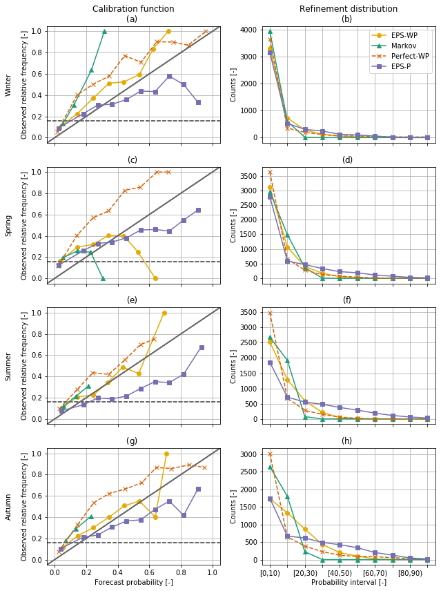
A key difference apparent from the calibration function relates to the ability of the models to identify subsets of forecast situations where the subsequent event relative frequencies are different, i.e. the forecast resolution. A fairly consistent feature across all lead times and drought classes is the poorer resolution of EPS-P, particularly obvious in summer (Figs. 10e and 11e), with the conditional event relative frequencies quite clearly closer to the climatological average compared to the other models. This should be considered in conjunction with the sharpness of the forecast, which is relatively high for this model as shown by the numbers of issued extreme probabilities, particularly those in the upper tail (Figs. 10f and 11f). This combination of poor resolution and high sharpness indicates “overconfidence” (Wilks, 2011) – on the occasions that EPS-P issues a forecast indicating the likelihood of a drought is very high, the actual likelihood of a drought subsequently occurring is lower. To compensate for this overconfidence, a user would adjust the probabilities to be less extreme to make the forecasts more reliable.
We can compare these refinement distributions to those of the Markov model, which exhibits low sharpness, overwhelmingly predicting droughts at the climatological frequency (second column of Figs. 10 and 11). This means that the Markov model is not a useful operational tool in these situations, as similar forecasts could be obtained simply by using the climatological drought frequency. The refinement distributions for EPS-WP show that for mild drought in winter and spring and for moderate drought in all seasons, the model predicts droughts with low probabilities the majority of the time (Figs. 10b and d and 11b, d, f and h). For mild drought in summer and autumn, however, this model mostly issues forecasts close to the climatological frequency, although not nearly as regularly as the Markov model (Fig. 10f and h). As with adjusting for bias, a forecaster can use model resolution and sharpness when assessing drought forecast probabilities output by a model.
We have compared the performance of a dynamical forecast system (EPS-WP) and a first-order Markov model in predicting WP occurrences over a range of lead times, showing that the dynamical model is always more skilful, although the difference in skill reduces with lead time. From these WP predictions, we derived precipitation and meteorological drought forecasts and compared them to direct precipitation and drought predictions from the dynamical system (EPS-P). We compared two levels of drought: mild drought, when the total precipitation over the lead time (16, 31 or 46 d) was below the 30.9th percentile climatology, and moderate drought, when the total precipitation over the lead time was below the 15.9th percentile. Overall, forecast models were found to be more skilful during winter and autumn, particularly for longer lead times. The Markov model tended to be the least skilful, especially when predicting drought. Differences in skill between EPS-P and EPS-WP were typically small, with RPSS, BSS and ROC results not highlighting a clear winner. However, we demonstrated the potential in improving WP forecasts further by showing that an idealised, perfect-prognosis model (Perfect-WP) would provide much more skilful precipitation and drought forecasts, with high hit rates and low false alarm rates.
From assessing reliability diagrams, we found that WP-based models only issue binary drought forecasts with either very low probabilities or probabilities close to the climatological average. In particular, there is little to gain in using the Markov model in mild drought prediction over the climatological frequency, as it tends to issue drought forecasts with this probability anyway. EPS-P has the highest sharpness, predicting drought occurrence with a wide range of probabilities. In particular, it issues greater numbers of high-probability drought forecasts compared to WP-based methods. However, this model also has poor resolution, indicating that it is an overconfident forecast model. Overall, drought forecasts issued by EPS-WP are the most reliable, i.e. the forecast probabilities are most similar to the subsequent event probabilities (they “mean what they say”; Wilks, 2011). Perfect-WP tends to under-forecast the number of drought events, while EPS-P over-forecasts drought events, particularly for moderate drought. These reliability diagrams are therefore useful for aiding users in adjusting for an over- or under-forecasting bias.
The higher skill of EPS-WP during winter (and possibly autumn) is probably due to the typically higher skill that medium- to long-range dynamical forecast systems have in predicting atmospheric variables in this season compared to other seasons (Scaife et al., 2014; MacLachlan et al., 2015; Neal et al., 2016; Arnal et al., 2018). In fact, by forecasting a set of eight WPs derived from MO30, Neal et al. (2016) found that ECMWF-EPS exhibited greater skill in winter than summer. Furthermore, the relationship between the NAO (which is the primary mode of North Atlantic–European atmospheric circulation) and precipitation is stronger in this season (Hurrell and Deser, 2009; Lavers et al., 2010; Svensson et al., 2015). This is particularly true for western regions (Jones et al., 2013; van Oldenborgh et al., 2015; Svensson et al., 2015; Hall and Hanna, 2018), which potentially explains the greater skill of precipitation and drought forecasting using observed WPs (Perfect-WP). The regional variations in skill of this model imply that MO30 is not as suited for representing precipitation in the east. Perhaps this is because the WPs are more closely related to the NAO in this season compared to other teleconnection patterns. As Hall and Hanna (2018) showed, the NAO is not the only important teleconnection pattern influencing UK precipitation.
By analysing the skill of an idealised “forecast” model that assumes perfect WP predictions, we have demonstrated the potential for using WP forecasts to derive precipitation and drought predictions. The skill of this model during winter and autumn suggests that the processes between the WPs and precipitation are well represented in these seasons. The lesser skill of EPS-WP and Markov, then, is a result of poor prediction of the WPs. A focus on improving the skill of the WP forecasts could be the most useful route to improving precipitation and drought predicting skill. Currently, dynamical models such as the ECMWF system used here represent the best method of predicting WPs. Moreover, the ECMWF reforecast data used here had 11 ensemble members, whereas the operational forecasts are run with 51 members. Therefore, an operationalised version of the models might improve forecast skill or better represent uncertainty, although this is also true for precipitation forecasts direct from the model. A useful piece of further research would be to assess the forecast skill of other models, and multi-model ensembles, at predicting MO30 WPs or other WP classification systems. Another potential method to improve precipitation and drought forecast skill would be to alter the process by which precipitation is estimated from the WPs. Here we sampled from the entire conditional distribution of precipitation given the WP and season, but this may not be the optimal way of estimation. It is possible that other factors influence the precipitation from WPs, such as slowly varying atmospheric and oceanic processes. For example, it would be interesting to see if conditioning the distributions further on the state of the NAO index, or some North Atlantic SST index, and sampling precipitation from these, would improve forecast skill. This is potentially most useful in predicting moderate drought, for which skill from current models is lower than for mild drought.
The code is only available locally with DR. Please contact the corresponding author for any queries regarding sharing the code.
Met Office EMULATE MSLP data (Ansell et al., 2006) can be found at https://www.metoffice.gov.uk/hadobs/emslp/data/download.html (last access: January 2020), ERA-Interim data at https://apps.ecmwf.int/datasets/data/interim-full-daily/levtype=sfc/ (last access: January 2020), ECMWF EPS hindcast data at https://apps.ecmwf.int/datasets/data/s2s-reforecasts-instantaneous-accum-ecmf/levtype=sfc/type=cf/ (last access: January 2020) and Met Office HadUKP data at https://www.metoffice.gov.uk/hadobs/hadukp/data/download.html (last access: January 2020).
The supplement related to this article is available online at: https://doi.org/10.5194/nhess-20-107-2020-supplement.
DR was the primary designer of the experiment, developed the model code, produced the figures and wrote the paper. HJF, CGK, RN and RD contributed to the design of the experiment and provided input to figure and text editing.
The authors declare that they have no conflict of interest.
This article is part of the special issue “Recent advances in drought and water scarcity monitoring, modelling, and forecasting (EGU2019, session HS4.1.1/NH1.31)”. It is a result of the European Geosciences Union General Assembly 2019, Vienna, Austria, 7–12 April 2019.
We thank two reviewers for their insightful comments and suggestions that improved the quality of this article. This work was part of a NERC-funded Postgraduate Research Student Studentship NE/L010518/1. Hayley J. Fowler is funded by the Wolfson Foundation and the Royal Society as a Royal Society Wolfson Research Merit Award (WM140025) holder. Hayley J. Fowler acknowledges support from the INTENSE project supported by the European Research Council (grant ERC-2013-CoG-617329).
This research has been supported by the Natural Environment Research Council (grant no. NE/L010518/1), the European Research Council (grant no. ERC‐2013‐CoG‐617329) and the Wolfson Foundation (grant no. WM140025).
This paper was edited by Brunella Bonaccorso and reviewed by Christophe Lavaysse and Massimiliano Zappa.
Ahrens, B. and Walser, A.: Information-Based Skill Scores for Probabilistic Forecasts, Mon. Weather Rev., 136, 352–363, https://doi.org/10.1175/2007mwr1931.1, 2008.
Alexander, L. V. and Jones, P. D.: Updated Precipitation Series for the U.K. and Discussion of Recent Extremes, Atmos. Sci. Lett., 1, 142–150, 2000.
Ansell, T. J., Jones, P. D., Allan, R. J., Lister, D., Parker, D. E., Brunet, M., Moberg, A., Jacobeit, J., Brohan, P., Rayner, N. A., Aguilar, E., Alexandersson, H., Barriendos, M., Brandsma, T., Cox, N. J., Della-Marta, P. M., Drebs, A., Founda, D., Gerstengarbe, F., Hickey, K., Jónsson, T., Luterbacher, J. Ø. N., Oesterle, H., Petrakis, M., Philipp, A., Rodwell, M. J., Saladie, O., Sigro, J., Slonosky, V., Srnec, L., Swail, V., García-Suárez, A. M., Tuomenvirta, H., Wang, X., Wanner, H., Werner, P., Wheeler, D., and Xoplaki, E.: Daily Mean Sea Level Pressure Reconstructions for the European–North Atlantic Region for the Period 1850–2003, J. Climate, 19, 2717–2742, https://doi.org/10.1175/jcli3775.1, 2006.
Arnal, L., Cloke, H. L., Stephens, E., Wetterhall, F., Prudhomme, C., Neumann, J., Krzeminski, B., and Pappenberger, F.: Skilful seasonal forecasts of streamflow over Europe?, Hydrol. Earth Syst. Sci., 22, 2057–2072, https://doi.org/10.5194/hess-22-2057-2018, 2018.
Baker, L. H., Shaffrey, L. C., and Scaife, A. A.: Improved seasonal prediction of UK regional precipitation using atmospheric circulation, Int. J. Climatol., 38, 437–453, https://doi.org/10.1002/joc.5382, 2018.
Bárdossy, A. and Filiz, F.: Identification of flood producing atmospheric circulation patterns, J. Hydrol., 313, 48–57, https://doi.org/10.1016/j.jhydrol.2005.02.006, 2005.
Brier, G. W.: Verification of forecasts expressed in terms of probability, Mon. Weather Rev., 78, 1–3, https://doi.org/10.1175/1520-0493(1950)078<0001:vofeit>2.0.co;2, 1950.
Brigode, P., Gérardin, M., Bernardara, P., Gailhard, J., and Ribstein, P.: Changes in French weather pattern seasonal frequencies projected by a CMIP5 ensemble, Int. J. Climatol., 38, 3991–4006, https://doi.org/10.1002/joc.5549, 2018.
Bröcker, J. and Smith, L., A.: Increasing the Reliability of Reliability Diagrams, Weather Forecast., 22, 651–661, https://doi.org/10.1175/waf993.1, 2007.
Buizza, R., Bidlot, J.-R., Wedi, N., Fuentes, M., Hamrud, M., Holt, G., and Vitart, F.: The new ECMWF VAREPS (Variable Resolution Ensemble Prediction System), Q. J. Roy. Meteorol. Soc., 133, 681–695, https://doi.org/10.1002/qj.75, 2007.
Cuo, L., Pagano, T. C., and Wang, Q. J.: A Review of Quantitative Precipitation Forecasts and Their Use in Short- to Medium-Range Streamflow Forecasting, J. Hydrometeorol., 12, 713–728, https://doi.org/10.1175/2011jhm1347.1, 2011.
Dee, D. P., Uppala, S. M., Simmons, A. J., Berrisford, P., Poli, P., Kobayashi, S., Andrae, U., Balmaseda, M. A., Balsamo, G., Bauer, P., Bechtold, P., Beljaars, A. C. M., van de Berg, L., Bidlot, J., Bormann, N., Delsol, C., Dragani, R., Fuentes, M., Geer, A. J., Haimberger, L., Healy, S. B., Hersbach, H., Hólm, E. V., Isaksen, L., Kållberg, P., Köhler, M., Matricardi, M., McNally, A. P., Monge-Sanz, B. M., Morcrette, J. J., Park, B. K., Peubey, C., de Rosnay, P., Tavolato, C., Thépaut, J. N., and Vitart, F.: The ERA-Interim reanalysis: configuration and performance of the data assimilation system, Q. J. Roy. Meteorol. Soc., 137, 553–597, https://doi.org/10.1002/qj.828, 2011.
Dutra, E., Di Giuseppe, F., Wetterhall, F., and Pappenberger, F.: Seasonal forecasts of droughts in African basins using the Standardized Precipitation Index, Hydrol. Earth Syst. Sci., 17, 2359–2373, https://doi.org/10.5194/hess-17-2359-2013, 2013.
ECMWF: Model Description CY43R1, available at: https://confluence.ecmwf.int/display/S2S/ECMWF+Model+Description+CY43R1 (last access: 3 June 2018), 2017.
Epstein, E. S. : A Scoring System for Probability Forecasts of Ranked Categories, J. Appl. Meteorol., 8, 985–987, https://doi.org/10.1175/1520-0450(1969)008<0985:assfpf>2.0.co;2, 1969.
Ferranti, L., Corti, S., and Janousek, M.: Flow-dependent verification of the ECMWF ensemble over the Euro-Atlantic sector, Q. J. Roy. Meteorol. Soc., 141, 916–924, https://doi.org/10.1002/qj.2411, 2015.
Golding, B. W.: Quantitative precipitation forecasting in the UK, J. Hydrol., 239, 286–305, https://doi.org/10.1016/S0022-1694(00)00354-1, 2000.
Hall, R. J. and Hanna, E.: North Atlantic circulation indices: links with summer and winter UK temperature and precipitation and implications for seasonal forecasting, Int. J. Climatol., 38, e660–e677, https://doi.org/10.1002/joc.5398, 2018.
Hannaford, J., Lloyd-Hughes, B., Keef, C., Parry, S., and Prudhomme, C.: Examining the large-scale spatial coherence of European drought using regional indicators of precipitation and streamflow deficit, Hydrol. Process., 25, 1146–1162, https://doi.org/10.1002/hyp.7725, 2011.
Hay, L. E., McCabe, G. J., Wolock, D. M., and Ayers, M. A.: Simulation of precipitation by weather type analysis, Water Resour. Res., 27, 493–501, https://doi.org/10.1029/90WR02650, 1991.
Hay, L. E., McCabe, G. J., Wolock, D. M., and Ayers, M. A.: Use of weather types to disaggregate general circulation model predictions, J. Geophys. Res.-Atmos., 97, 2781–2790, https://doi.org/10.1029/91JD01695, 1992.
Hurrell, J. W. and Deser, C.: North Atlantic climate variability: The role of the North Atlantic Oscillation, J. Mar. Syst., 78, 28–41, https://doi.org/10.1016/j.jmarsys.2008.11.026, 2009.
Huth, R., Beck, C., Philipp, A., Demuzere, M., Ustrnul, Z., Cahynová, M., Kyselý, J., and Tveito, O. E.: Classifications of Atmospheric Circulation Patterns, Ann. NY Acad. Sci., 1146, 105–152, https://doi.org/10.1196/annals.1446.019, 2008.
Jones, M. R., Fowler, H. J., Kilsby, C. G., and Blenkinsop, S.: An assessment of changes in seasonal and annual extreme rainfall in the UK between 1961 and 2009, Int. J. Climatol., 33, 1178–1194, https://doi.org/10.1002/joc.3503, 2013.
Kendon, M., Marsh, T., and Parry, S.: The 2010–2012 drought in England and Wales, Weather, 68, 88–95, https://doi.org/10.1002/wea.2101, 2013.
Kharin, V. V. and Zwiers, F. W.: Improved Seasonal Probability Forecasts, J. Climate, 16, 1684–1701, https://doi.org/10.1175/1520-0442(2003)016<1684:ispf>2.0.co;2, 2003.
Kleeman, R.: Measuring Dynamical Prediction Utility Using Relative Entropy, J. Atmos. Sci., 59, 2057–2072, https://doi.org/10.1175/1520-0469(2002)059<2057:mdpuur>2.0.co;2, 2002.
Kullback, S. and Leibler, R. A.: On Information and Sufficiency, Ann. Math. Stat., 22, 79–86, https://doi.org/10.1214/aoms/1177729694, 1951.
Lavaysse, C., Vogt, J., and Pappenberger, F.: Early warning of drought in Europe using the monthly ensemble system from ECMWF, Hydrol. Earth Syst. Sci., 19, 3273–3286, https://doi.org/10.5194/hess-19-3273-2015, 2015.
Lavaysse, C., Vogt, J., Toreti, A., Carrera, M. L., and Pappenberger, F.: On the use of weather regimes to forecast meteorological drought over Europe, Nat. Hazards Earth Syst. Sci., 18, 3297–3309, https://doi.org/10.5194/nhess-18-3297-2018, 2018.
Lavers, D. A., Prudhomme, C., and Hannah, D. M.: Large-scale climate, precipitation and British river flows: Identifying hydroclimatological connections and dynamics, J. Hydrol., 395, 242–255, https://doi.org/10.1016/j.jhydrol.2010.10.036, 2010.
Lavers, D. A., Pappenberger, F., and Zsoter, E.: Extending medium-range predictability of extreme hydrological events in Europe, Nat. Commun., 5, 5382, https://doi.org/10.1038/ncomms6382, 2014.
Lavers, D. A., Waliser, D. E., Ralph, F. M., and Dettinger, M. D.: Predictability of horizontal water vapor transport relative to precipitation: Enhancing situational awareness for forecasting western U.S. extreme precipitation and flooding, Geophys. Res. Lett., 43, 2275–2282, https://doi.org/10.1002/2016GL067765, 2016.
Leung, L.-Y. and North, G., R.: Information Theory and Climate Prediction, J. Climate, 3, 5–14, https://doi.org/10.1175/1520-0442(1990)003<0005:itacp>2.0.co;2, 1990.
Lin, J.: Divergence measures based on the Shannon entropy, IEEE T. Inform. Theory, 37, 145–151, https://doi.org/10.1109/18.61115, 1991.
MacLachlan, C., Arribas, A., Peterson, K. A., Maidens, A., Fereday, D., Scaife, A. A., Gordon, M., Vellinga, M., Williams, A., Comer, R. E., Camp, J., Xavier, P., and Madec, G.: Global Seasonal forecast system version 5 (GloSea5): a high-resolution seasonal forecast system, Q. J. Roy. Meteorol. Soc., 141, 1072–1084, https://doi.org/10.1002/qj.2396, 2015.
Marsh, T., Cole, G., and Wilby, R.: Major droughts in England and Wales, 1800–2006, Weather, 62, 87–93, https://doi.org/10.1002/wea.67, 2007.
Marsh, T. J. and Turton, P. S.: The 1995 drought – a water resources perspective, Weather, 51, 46–53, https://doi.org/10.1002/j.1477-8696.1996.tb06184.x, 1996.
Mason, I.: A model for assessment of weather forecasts, Aust. Meteorol. Mag., 30, 291–303, 1982.
McKee, T. B., Doesken, N. J., and Kleist, J.: The relationship of drought frequency and duration to time scales, in: Proceedings of the 8th Conference on Applied Climatology, 17–22 January 1993, Anaheim, California, 1993.
Murphy, A. H.: A Note on the Ranked Probability Score, J. Appl. Meteorol., 10, 155–156, https://doi.org/10.1175/1520-0450(1971)010<0155:anotrp>2.0.co;2, 1971.
Murphy, A. H.: A New Vector Partition of the Probability Score, J. Appl. Meteorol., 12, 595–600, https://doi.org/10.1175/1520-0450(1973)012<0595:anvpot>2.0.co;2, 1973.
Mwangi, E., Wetterhall, F., Dutra, E., Di Giuseppe, F., and Pappenberger, F.: Forecasting droughts in East Africa, Hydrol. Earth Syst. Sci., 18, 611–620, https://doi.org/10.5194/hess-18-611-2014, 2014.
Neal, R., Fereday, D., Crocker, R., and Comer, R. E.: A flexible approach to defining weather patterns and their application in weather forecasting over Europe, Meteorol. Appl., 23, 389–400, https://doi.org/10.1002/met.1563, 2016.
Neal, R., Dankers, R., Saulter, A., Lane, A., Millard, J., Robbins, G., and Price, D.: Use of probabilistic medium- to long-range weather-pattern forecasts for identifying periods with an increased likelihood of coastal flooding around the UK, Meteorol. Appl., 25, 534–547, https://doi.org/10.1002/met.1719, 2018.
Nigro, M. A., Cassano, J. J., and Seefeldt, M. W.: A Weather-Pattern-Based Approach to Evaluate the Antarctic Mesoscale Prediction System (AMPS) Forecasts: Comparison to Automatic Weather Station Observations, Weather Forecast., 26, 184–198, https://doi.org/10.1175/2010waf2222444.1, 2011.
Richardson, D., Fowler, H. J., Kilsby, C. G., and Neal, R.: A new precipitation and drought climatology based on weather patterns, Int. J. Climatol., 38, 630–648, https://doi.org/10.1002/joc.5199, 2018.
Richardson, D., Kilsby, C. G., Fowler, H. J., and Bárdossy, A.: Weekly to multi-month persistence in sets of daily weather patterns over Europe and the North Atlantic Ocean, Int. J. Climatol., 39, 2041–2056, https://doi.org/10.1002/joc.5932, 2019a.
Richardson, D., Neal, R., Dankers, R., Mylne, K., Cowling, R., Clements, H., and Millard, J.: Linking weather patterns to regional extreme precipitation for highlighting potential flood events in medium- to long-range forecasts, Meteorol. Appl., in review, 2019b.
Rodda, J. C. and Marsh, T. J.: The 1975–76 Drought – a contemporary and retrospective review, available at: http://www.ceh.ac.uk/data/nrfa/nhmp/other_reports/CEH_1975-76_Drought_Report_Rodda_and_Marsh.pdf (last access: 23 February 2019), 2011.
Roulston, M. S. and Smith, L. A.: Evaluating Probabilistic Forecasts Using Information Theory, Mon. Weather Rev., 130, 1653–1660, https://doi.org/10.1175/1520-0493(2002)130<1653:epfuit>2.0.co;2, 2002.
Saha, S., Shrinivas, M., Xingren, W., Jiande, W., Sudhir, N., Patrick, T., David, B., Yu-Tai, H., Hui-ya, C., Mark, I., Michael, E., Jesse, M., Rongqian, Y., Malaquías Peña, M., Huug van den, D., Qin, Z., Wanqiu, W., Mingyue, C., and Emily, B.: The NCEP Climate Forecast System Version 2, J. Climate, 27, 2185–2208, https://doi.org/10.1175/jcli-d-12-00823.1, 2014.
Scaife, A. A., Arribas, A., Blockley, E., Brookshaw, A., Clark, R. T., Dunstone, N., Eade, R., Fereday, D., Folland, C. K., Gordon, M., Hermanson, L., Knight, J. R., Lea, D. J., MacLachlan, C., Maidens, A., Martin, M., Peterson, A. K., Smith, D., Vellinga, M., Wallace, E., Waters, J., and Williams, A.: Skillful long-range prediction of European and North American winters, Geophys. Res. Lett., 41, 2514–2519, https://doi.org/10.1002/2014GL059637, 2014.
Smith, D. M., Scaife, A. A., and Kirtman, B. P.: What is the current state of scientific knowledge with regard to seasonal and decadal forecasting?, Environ. Res. Lett., 7, 015602, https://doi.org/10.1088/1748-9326/7/1/015602, 2012.
Svensson, C., Brookshaw, A., Scaife, A. A., Bell, V. A., Mackay, J. D., Jackson, C. R., Hannaford, J., Davies, H. N., Arribas, A., and Stanley, S.: Long-range forecasts of UK winter hydrology, Environ. Res. Lett., 10, 064006, https://doi.org/10.1088/1748-9326/10/6/064006, 2015.
van Oldenborgh, G. J., Stephenson, D. B., Sterl, A., Vautard, R., Yiou, P., Drijfhout, S. S., von Storch, H., and van den Dool, H.: Drivers of the 2013/14 winter floods in the UK, Nat. Clim. Change, 5, 490–491, https://doi.org/10.1038/nclimate2612, 2015.
Vitart, F.: Evolution of ECMWF sub-seasonal forecast skill scores, Q. J. Roy. Meteorol. Soc., 140, 1889–1899, https://doi.org/10.1002/qj.2256, 2014.
Vitart, F., Buizza, R., Alonso Balmaseda, M., Balsamo, G., Bidlot, J.-R., Bonet, A., Fuentes, M., Hofstadler, A., Molteni, F., and Palmer, T. N.: The new VarEPS-monthly forecasting system: A first step towards seamless prediction, Q. J. Roy. Meteorol. Soc., 134, 1789–1799, https://doi.org/10.1002/qj.322, 2008.
Vitart, F., Ardilouze, C., Bonet, A., Brookshaw, A., Chen, M., Codorean, C., Déqué, M., Ferranti, L., Fucile, E., Fuentes, M., Hendon, H., Hodgson, J., Kang, H.-S., Kumar, A., Lin, H., Liu, G., Liu, X., Malguzzi, P., Mallas, I., Manoussakis, M., Mastrangelo, D., MacLachlan, C., McLean, P., Minami, A., Mladek, R., Nakazawa, T., Najm, S., Nie, Y., Rixen, M., Robertson, A. W., Ruti, P., Sun, C., Takaya, Y., Tolstykh, M., Venuti, F., Waliser, D., Woolnough, S., Wu, T., Won, D.-J., Xiao, H., Zaripov, R., and Zhang, L.: The Subseasonal to Seasonal (S2S) Prediction Project Database, B. Am. Meteorol. Soc., 98, 163–173, https://doi.org/10.1175/bams-d-16-0017.1, 2017.
Vuillaume, J.-F. and Herath, S.: Improving global rainfall forecasting with a weather type approach in Japan, Hydrolog. Sci. J., 62, 167–181, https://doi.org/10.1080/02626667.2016.1183165, 2017.
Walker, G. T. and Bliss, E. W.: World Weather V, Memoir. Roy. Meteorol. Soc., 4, 53–84, 1932.
Wedgbrow, C. S., Wilby, R. L., Fox, H. R., and O'Hare, G.: Prospects for seasonal forecasting of summer drought and low river flow anomalies in England and Wales, Int. J. Climatol., 22, 219–236, https://doi.org/10.1002/joc.735, 2002.
Wedgbrow, C. S., Wilby, R., and Fox, H. R.: Experimental seasonal forecasts of low summer flows in the River Thames, UK, using Expert Systems, Clim. Res., 28, 133–141, https://doi.org/10.3354/cr028133, 2005.
Weijs, S. V. and v. d. Giesen, N.: Accounting for Observational Uncertainty in Forecast Verification: An Information-Theoretical View on Forecasts, Observations, and Truth, Mon. Weather Rev., 139, 2156–2162, https://doi.org/10.1175/2011mwr3573.1, 2011.
Weijs, S. V., v. Nooijen, R., and v. d. Giesen, N.: Kullback–Leibler Divergence as a Forecast Skill Score with Classic Reliability–Resolution–Uncertainty Decomposition, Mon. Weather Rev., 138, 3387–3399, https://doi.org/10.1175/2010mwr3229.1, 2010.
Wilby, R. L.: Stochastic weather type simulation for regional climate change impact assessment, Water Resour. Res., 30, 3395–3403, https://doi.org/10.1029/94WR01840, 1994.
Wilby, R. L.: Modelling low-frequency rainfall events using airflow indices, weather patterns and frontal frequencies, J. Hydrol., 212–213, 380–392, https://doi.org/10.1016/S0022-1694(98)00218-2, 1998.
Wilks, D. S.: Chapter 7 Forecast verification, in: International Geophysics, edited by: Wilks, D. S., Academic Press, San Diego, USA, 233–283, 1995.
Wilks, D. S.: Chapter 8 – Forecast Verification, in: International Geophysics, edited by: Wilks, D. S., Academic Press, San Diego, USA, 301–394, 2011.
Yoon, J.-H., Mo, K., and Wood, E. F.: Dynamic-Model-Based Seasonal Prediction of Meteorological Drought over the Contiguous United States, J. Hydrometeorol., 13, 463–482, https://doi.org/10.1175/jhm-d-11-038.1, 2012.
Yuan, X. and Wood, E. F.: Multimodel seasonal forecasting of global drought onset, Geophys. Res. Lett., 40, 4900–4905, https://doi.org/10.1002/grl.50949, 2013.