the Creative Commons Attribution 4.0 License.
the Creative Commons Attribution 4.0 License.
 | 17 Apr 2019
Probabilistic forecasting of plausible debris flows from Nevado de Colima (Mexico) using data from the Atenquique debris flow, 1955
Andrea Bevilacqua
Abani K. Patra
Marcus I. Bursik
E. Bruce Pitman
José Luis Macías
Ricardo Saucedo
David Hyman
We detail a new prediction-oriented procedure aimed at volcanic hazard assessment based on geophysical mass flow models constrained with heterogeneous and poorly defined data. Our method relies on an itemized application of the empirical falsification principle over an arbitrarily wide envelope of possible input conditions. We thus provide a first step towards a objective and partially automated experimental design construction. In particular, instead of fully calibrating model inputs on past observations, we create and explore more general requirements of consistency, and then we separately use each piece of empirical data to remove those input values that are not compatible with it. Hence, partial solutions are defined to the inverse problem. This has several advantages compared to a traditionally posed inverse problem: (i) the potentially nonempty inverse images of partial solutions of multiple possible forward models characterize the solutions to the inverse problem; (ii) the partial solutions can provide hazard estimates under weaker constraints, potentially including extreme cases that are important for hazard analysis; (iii) if multiple models are applicable, specific performance scores against each piece of empirical information can be calculated. We apply our procedure to the case study of the Atenquique volcaniclastic debris flow, which occurred on the flanks of Nevado de Colima volcano (Mexico), 1955. We adopt and compare three depth-averaged models currently implemented in the TITAN2D solver, available from https://vhub.org (Version 4.0.0 – last access: 23 June 2016). The associated inverse problem is not well-posed if approached in a traditional way. We show that our procedure can extract valuable information for hazard assessment, allowing the exploration of the impact of synthetic flows that are similar to those that occurred in the past but different in plausible ways. The implementation of multiple models is thus a crucial aspect of our approach, as they can allow the covering of other plausible flows. We also observe that model selection is inherently linked to the inversion problem.
- Article
(12388 KB) - Full-text XML
-
Supplement
(38527 KB) - BibTeX
- EndNote


Hazard assessment of geophysical mass flows, such as landslides or pyroclastic flows, usually relies on the reconstruction of past flows that occurred in the region of interest using models of physics that have been successful in hindcasting. The available pieces of data Di∈𝒟, are commonly related to the properties of the deposit left by the flows and to historical documentation. In general, this information can be affected by relevant sources of uncertainty (e.g., erosion and remobilization, superposition of subsequent events, unknown duration, and source). Physical models provide us with a deterministic system to relate inputs and outputs of the dynamical system of the mass flow (Gilbert, 1991; Patra et al., 2018a) and are traditionally used to explore “what if” scenarios and more recently in ways to supplement observed data with physically consistent synthetic data (Bayarri et al., 2015) for probabilistic analysis. However, this relation is dependent on the difficult choice of a model and parameters for future events.
In a probabilistic framework, for each model M∈ℳ we define (M, PM), where PM is a probability measure over the parameter space of M. While the support of PM can be restricted to a single value by solving an inverse problem for the optimal reconstruction of a particular flow, the inverse problem is not always well posed. That is, no input data or multiple input data are able to produce outputs consistent with the observed information (Tarantola and Valette, 1982; Tarantola, 1987). Choices based on limited data using classical inversion are often misleading since they do not reflect all potential event characteristics and can be error prone due to incorrectly limited event space. Sometimes the strict replication of a past flow may lead to overconstraining the model, especially if we are interested in the general predictive capabilities of a model over a whole range of possible future events. In this study, we use a multi-model ensemble and a plausible region approach to provide a more prediction-oriented probabilistic framework for hazard analysis. In particular, we generalize a poorly constrained inverse problem, decomposing it into a hierarchy of simpler problems. We remark that our hazard assessment is related to plausible flows, similar to the event that occurred in 1955. A comprehensive hazard assessment for any kind of future debris flow event is beyond the scope of this work, though such an approach is likely a necessary element of any comprehensive future approach using diverse data.
1.1 Probabilistic description
Our approach is characterized by three steps:
-
For each model Mj∈ℳ, we initially set up a uniformly probabilized general input space that we define as arbitrarily wide, namely (, ). At this stage, we only require essential properties of feasibility in the models, namely the existence of the numerical output and the realism of the underlying physics. These initial input values are not subjectively incorporated or derived from literature or experiments.
-
After a preliminary screening, we characterize a specialized input space, , under additional requirements of plausibility1 that are related to the macroscopic properties of the outputs. For instance, a robust numerical simulation without spurious effects, meaningful flow dynamics, and/or the capability to inundate a designated region.
-
Through more detailed testing, , we can thus define the subspace of the inputs that are consistent with a piece of empirical data Di.
We remark that the specialized input space is the inverse image of the set of plausible outputs DG through the input–output functions fj characterizing the models (see following section). We also note that, ∀j, all the described subspaces of , if not negligible, are trivially probabilized by the measures Pj and , defined by
for each measurable set2 A.
The philosophy of our method is based on an itemized application of the empirical falsification principle of Karl Raimund Popper (Popper, 1959), over an arbitrarily wide envelope of possible input conditions. We remark that this statement is not related to the model selection effort but to the model inversion effort, i.e., to the iterative comparison of the members of a set of disparate data to the outputs of models. We use multiple models to cover a wider span of outputs, not to seek for a best model. Indeed, we empirically falsify portions of the input spaces, not the models forms themselves. The construction of the subspaces has several advantages compared to a traditionally posed inverse problem:
-
the intersection space describes the set of the inputs that solves the inverse problem;
-
the partial solutions provide information concerning flows that partially solve the inverse problem, and they may exist even if Θj=∅;
-
each probability represents a performance score of the adopted model against the piece of empirical data Di and can eventually be used for model comparison purposes, concerning that specific piece of data.
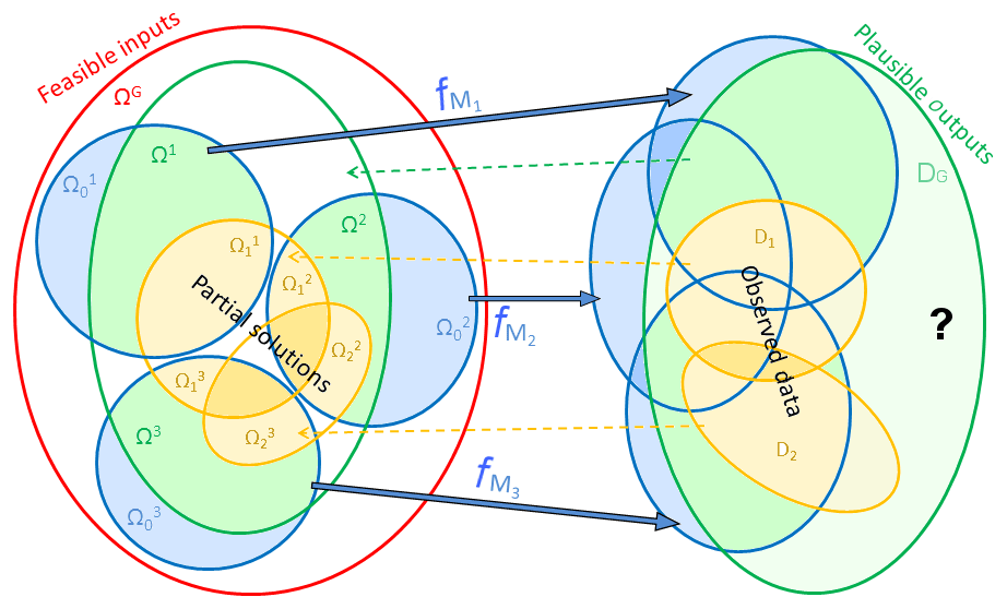
Figure 1Diagram of input spaces, model functions, and output space (blue), with feasible inputs domain (red), plausible output codomain and specialized inputs (green), and observed data and partial solutions subsets (orange). The question mark emphasizes that the covering of other plausible outputs could be enabled by adding more models if necessary.
1.2 Functional structures
Our meta-modeling framework is fully described in Fig. 1. Let us assume that each model Mj∈ℳ is represented by an operator:
where d∈ℕ is a dimensional parameter which is independent of the model chosen and characterizes a common output space. This operator simply links the input values in to the related output values in ℝd. We also define the global set of feasible inputs:
This puts all the models in a natural meta-modeling framework. Then, we characterize the codomain DG⊂ℝd of plausible outputs: that is, the target of our simulations – it includes all the outputs consistent with the observed data, plus additional outputs which differ in arbitrary but plausible ways. For the sake of simplicity, we use the same notation for each piece of data Di and the set of outputs consistent with it. Then ∀j, the specialized input space is defined by
That is, the set of all the feasible input values that produce plausible outputs. In a similar way, ∀i, , and for this reason those sets are called partial solutions to the inverse problem.
We remark that the implementation of multiple models is a crucial aspect in our approach. Typically, the available models are not able to entirely cover DG, and
That is, there are plausible outputs, and possibly observed data, that cannot be replicated by any of the considered models. The investigation of DG and the quality of the solutions will clearly improve as we add more models based on new knowledge of the underlying processes, especially when there is uncertainty as to which model is best in a particular situation. We show that the solution of the partial inverse problems and model selection are strongly linked.
1.3 Geophysical case study
We apply our procedure to the case study of the Atenquique volcaniclastic debris flow, which occurred on the flanks of Nevado de Colima volcano (Mexico) in 1955. We adopt and compare the three depth-averaged models Mohr–Coulomb (MC) (Savage and Hutter, 1989), Pouliquen–Forterre (PF) (Pouliquen, 1999; Pouliquen and Forterre, 2002; Forterre and Pouliquen, 2002), and Voellmy–Salm (VS) (Voellmy, 1955; Salm et al., 1990), based on the Saint Venant equations. Input spaces are explored by Monte Carlo simulation based on Latin hypercube sampling (McKay et al., 1979; Owen, 1992b; Stein, 1987; Ranjan and Spencer, 2014; Ai et al., 2016). The three models are incorporated in our large-scale mass flow simulation framework TITAN2D (Patra et al., 2005, 2006, 2018b; Yu et al., 2009; Aghakhani et al., 2016). So far, TITAN2D has been successfully applied to the simulation of different geophysical mass flows with specific characteristics (Sheridan et al., 2005, 2010; Rupp et al., 2006; Norini et al., 2009; Charbonnier and Gertisser, 2009; Procter et al., 2010; Sulpizio et al., 2010; Capra et al., 2011). Several studies involving TITAN2D were also directed towards a statistical study of geophysical flows, focusing on uncertainty quantification (Dalbey et al., 2008; Dalbey, 2009; Stefanescu et al., 2012a, b) or on the more efficient production of hazard maps (Bayarri et al., 2009, 2015; Spiller et al., 2014; Ogburn et al., 2016).
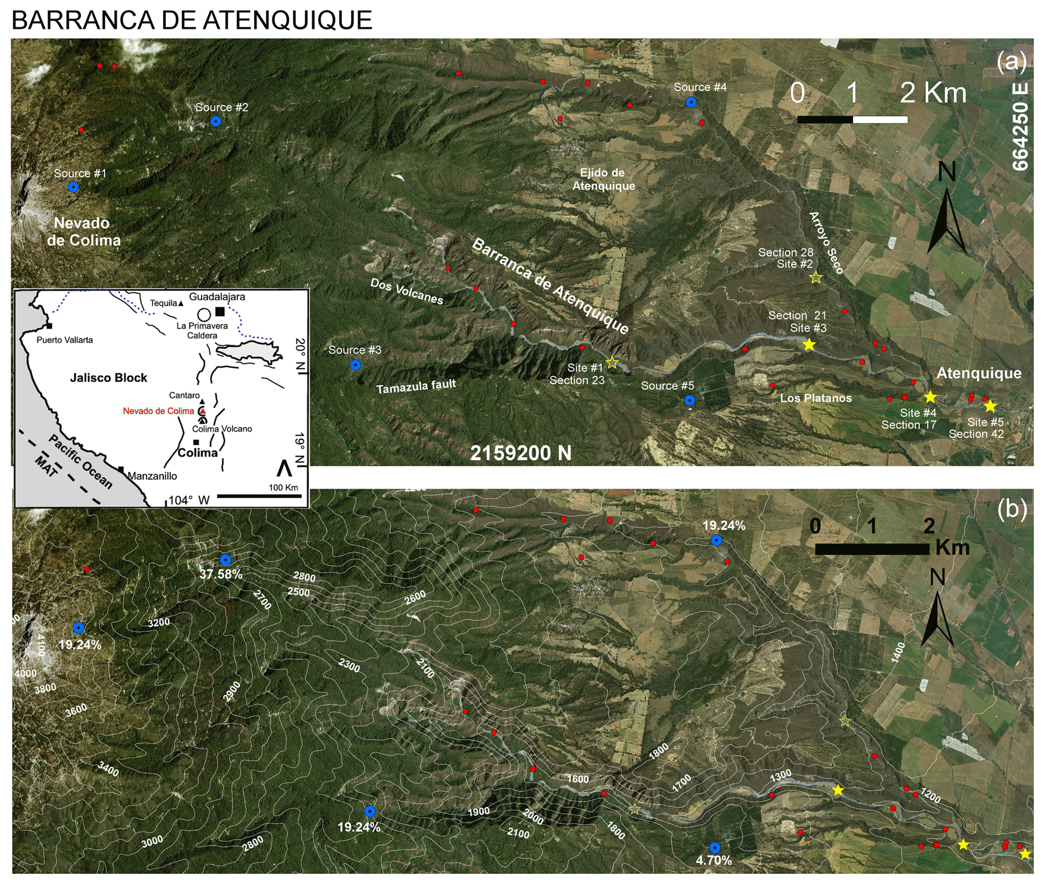
Figure 2Barranca de Atenquique (Mexico) overview. (a) Stratigraphic sections of Saucedo et al. (2008) are marked with red dots, including five preferred locations (yellow stars) and major ravines. Solid stars are detailed in the main text, and shaded stars are detailed in the Supplement. Initial source piles are marked by blue dots. Coordinates and projection are UTM zone 13∘ N WGS84. (b) Digital elevation map including isolines (NASA – JPL, 2014). Volume partition percentages among sources are reported. Regional map is included in a small box.
The rest of the study is organized as follows. In Sect. 2, we present our case study – debris flows from Nevado de Colima; in Sect. 3, we introduce the physical models, we define and parameterize their input spaces, and we design our Monte Carlo simulation; in Sect. 4 we statistically describe the characteristics of the outputs and contributing variables, mapping them globally and detailing them locally. Finally, in Sect. 5, we use multiple pieces of information regarding a historical debris flow to condition the input space, and then we compare the performance of the models over that space. The results show that model selection is inherently linked to the inversion problem: that is, model performance depends on which of the observed data we seek to reproduce. This is a fundamental aspect to consider in the development of multi-model solvers, dynamically selecting the model based on performance against local data.
The Colima Volcanic Complex is located in the western portion of the Trans-Mexican volcanic belt (small box in Fig. 2). It consists of a N–S volcanic chain formed by Cántaro, Nevado de Colima, and Colima volcanoes, within the Colima Graben (Luhr and Carmichael, 1990). It began forming 1.7 Ma ago with the growth of Cántaro volcano (2800 m a.s.l.) and continued with the formation of Nevado de Colima volcano 0.53 Ma ago (Allan, 1986; Robin et al., 1987). Activity was intermittent during the Pleistocene and Holocene and continues today at Colima volcano (3860 m a.s.l.), south of Nevado (Saucedo et al., 2010; Zobin et al., 2015; Macorps et al., 2018).
Nevado de Colima (4320 m a.s.l.) occupies the central part of the volcanic complex, being the most voluminous of the three volcanoes (300–400 km3). It is characterized by three or four horseshoe-shaped craters (Cortés et al., 2010). The youngest crater is 4 km wide and opens to the east with 100 m deep, vertical walls. This structure contains the summit Picacho dome (4300 m). The eastern flank of Nevado exposes a thick sequence of debris flow, fluvial, pyroclastic flow and debris avalanche deposits known as the Atenquique Formation (Mooser, 1961; Cortés et al., 2005; Saucedo et al., 2008), covered by younger deposits. The crater morphology directs a large part of the drainage from the volcano into the Atenquique ravine, located on the ENE flank of the volcano and ∼25 km long. Figure 2 shows the ravine and its surrounding topography.
Figure 2b includes elevation isolines from the SRTM DEM of 30 m cell size for UTM zone 13∘ N (NASA – JPL, 2014). The drainage begins at an elevation of 4000 m on the eastern flank of Nevado, is occupied by the perennial Atenquique River, and ends at its junction with the perennial Tuxpan River at 1040 m. Between 4000 and 2000 m in altitude, the ravine has an average slope of 34∘. At an elevation of 1800 m, the Atenquique ravine is cut off by a 250 m cliff in the vicinity of the junction with the Dos Volcanes dry ravine. Beyond this cliff, the slope of the ravine suddenly decreases from 34 to 18∘, keeping this gradient to an elevation of 1600 m at 11.5 km from the summit. Between this site and the catchments of the Los Plátanos and Arroyo Seco dry ravines, located at ∼21.5 m at an elevation of 1120 m, the ravine gradient varies from 10 to 6∘. The town of Atenquique is located at an altitude of 1050 m and 18.5 km (25 km along the ravine path) from the head of the ravine. There, the ravine channel has a gradient of 5∘, which is maintained down to the confluence with the Tuxpan River. The Atenquique ravine has an average width of 30 m, although in the vicinity of Atenquique village it is up to 200 m wide.
2.1 The Atenquique volcaniclastic debris flow, 1955
On 16 October 1955, at 10:45 LT, the inhabitants of Atenquique were surprised by the sudden arrival of an 8–9 m high wave carrying mud, boulders and tree trunks that devastated the buildings in the town and four bridges, including the railroad bridge. More than 23 people died, and the flood leveled everything but the tower of the church and the upper part of the market place that luckily served as shelter for survivors (Ponce-Segura, 1983; Saucedo et al., 2008). During the peak flow, eyewitnesses observed that complete walls of buildings were displaced several meters by the flood prior to their collapse. The deposits are exposed along the Atenquique, Arroyo Seco, Los Plátanos, and Dos Volcanes ravines, and their distribution, stratigraphy, granulometry, and volume have been described in Saucedo et al. (2008). Sixty stratigraphic sections were studied along the Atenquique ravine and its main tributaries (Fig. 2). Deposits cover a minimal area of 1.2 km2, and a minimum volume of 3.2×10⁶ m3 was estimated for the flow.
The main flood probably formed in the Atenquique ravine but was enhanced by the confluence of flows from its tributaries: Dos Volcanes at 11.2 km, Arroyo Seco and Los Plátanos, at 22.5 km. The following description of the flow deposits summarizes Saucedo et al. (2008). We remark that we are not going to prescribe the rheology utilized in our modeling effort, rather, we will let the data guide us to plausible rheologies and inputs. During the first 10–12 km (as recorded by the proximal exposures) the flow moved down steep slopes, eroding and incorporating coarse alluvium and sand. It left a massive deposit with a polymodal grain-size distribution, with reverse grading of coarse clasts and features typical of noncohesive debris flows, suggesting a Mohr–Coulomb rheology might be appropriate. Downstream, in the medial exposures, the flow encountered gentler slopes, reducing its velocity and promoting deposition of part of the sediment load. The flow left a deposit with a bimodal grain-size distribution and better sorting than before. Dilution could have produced a change in the rheology, moving toward the boundary between a debris flow and a hyperconcentrated flow. Just upstream of the village, below the junction with the Arroyo Seco and Los Plátanos ravines, eyewitnesses reported peak flood levels, possibly enhanced by the engulfing of a small water reservoir. At the junction, the flow captured the fine-material load of flow from the Arroyo Seco and Plátanos ravines, causing significant dilution and a sudden increase in the flow turbulence and the capacity to transport coarse particles. The resulting deposit left by the flow entering Atenquique village again shows a polymodal grain-size distribution. Voellmy–Salm rheology might become more appropriate than Mohr–Coulomb. However, Pouliquen–Forterre rheology might also be able to flexibly reproduce the resulting behavior. Downstream from the town, the flow lost its capacity to transport large boulders, probably due to widening of the flow and the consequent fall in velocity, which may have been further reduced by the hydraulic roughness effects of the flow impacting buildings. The flood definitively transformed from a debris flow to a hyperconcentrated flow. The diluted flow probably had a peak velocity in the range of 4 to 6 m s−1, obtained using the methods of Pierson (1985). The flood finally continued downstream to join with the perennial Tuxpan River, where it eventually transformed to a sediment-laden flow. It emplaced up to 6 m of deposits.
2.2 Multiple sources and their locations
The 1955 debris flow, according to eyewitness accounts and deposit analyses, emanated from multiple sources throughout the watershed. The existence of multiple source areas presents a unique challenge when attempting to model the flow. Eyewitnesses confirm that, after the event, many small landslides scars were present along the main ravine and its tributaries. It is hypothesized that these landslides, triggered by rain infiltration, supplied the bulk of the material (Saucedo, 2003; Saucedo et al., 2008). To account for this and based on the work in Rupp (2004), we initiate the flow from five major source locations, reported in Fig. 2. We remark that our numerical simulation toolkit allows for multiple starting points in the same run. Each source consists of a paraboloid pile of material with a unitary aspect ratio. Two source locations (1 and 2) are placed in the main ravine, one (3) in a lateral valley associated with the regional Tamazula fault, one source (4) in Arroyo Seco and one (5) in Arroyo Plátanos. These locations are selected based on local topography. The first three are located on steep upland slopes, while the other two are located along the main drainage due to the lack of steep terrain nearby (Rupp, 2004). The partition of volume among the five sources is scaled based upon the size of the drainage basin they are located within. In particular, ∀k, we define as follows:
This is equivalent to choosing pile radii of 80, 100, and 50 m.
We remark that source number, location, and volume partition will be preserved in the following analysis. However, we tested whether small variations affect the character of the simulated flow only proximally. Large variations, for example additional testing focused on increasing the weight w4 of the source in Arroyo Seco are not excluded but would require additional field work to be constrained and are beyond the purpose of this study. More details about volume V are provided in Sect. 3.1.
Our numerical modeling of the Atenquique flow proceeds by first assuming that the laws of mass and momentum conservation hold for properly defined system boundaries. The flow had very small depth compared to its length, and hence we assume that it is reasonable to integrate through the depth to obtain simpler and more computationally tractable equations (Savage and Hutter, 1989).
The depth-averaged Saint-Venant-type equations that result are as follows:
Here the Cartesian coordinate system is aligned such that z is normal to the surface; h is the flow depth in the z direction; and are respectively the components of momentum in the x and y directions; and k is the coefficient which relates the lateral stress components, and , to the normal stress component, . Note that is the contribution of hydrostatic pressure to the momentum fluxes. Sx and Sy are the sum local stresses: their definition depends on the constitutive model of the flowing material (Kelfoun, 2011). These include the gravitational driving forces, the basal friction force resisting to the motion of the material, and additional forces specific to the rheology assumptions.
In this study we adopt the Mohr–Coulomb (MC), Pouliquen–Forterre (PF), and Voellmy–Salm (VS) models, detailed in Appendix A. These three models for large-scale mass flows are incorporated in our large-scale mass flow simulation framework TITAN2D (Patra et al., 2005). The fourth release of TITAN2D3 offers multiple rheology options in the same code base. The availability of three distinct models for similar phenomena in the same tool provides us with the ability to directly compare outputs and internal variables in all the three models and control for usually difficult-to-quantify effects like numerical solution procedures, input ranges, and computer hardware (Patra et al., 2018b).
3.1 Preliminary definition of the input space
The definition of the input space hierarchy , ∀i, j, is a fundamental part of our approach. The dimensionality dj is a characteristic of the model. The input spaces of MC and VS have three dimensions and are therefore parameterized:
On the other hand, the input space of model PF originally has six dimensions – (ϕ1, ϕ2, ϕ3, β, L, V). Following Pouliquen and Forterre (2002), we constrain ∘. Moreover, preliminary testing in our case study showed a very similar impact from the variation of β and L. So, we were able to further reduce dPF=4, by assuming the empirical relationship
which is consistent with the β values presented in the literature (Pouliquen and Forterre, 2002; Forterre and Pouliquen, 2003). In the following we also show the effect of fixing the value of β. We thus effectively parameterize the following:
3.1.1 General input space
The input space boundaries , of are constrained by the following general assumptions:
-
Total volume: m3, i.e., m3.
-
Input space constraints:
∘, .
∘, , m.
∘, log 10(ξ)≤4.
In particular, a minimum volume of 3.2×10⁶ m3 for the deposit left by the flow was obtained by Saucedo et al. (2008). We assume that it is reasonable to increase this volume by about 10 % to 50 % to represent the potential real volume in the simulated flow, given the lack of recovery of any deposit for the portion of the flow reaching the Tuxpan River. We exclude basal friction angles below 5∘ in MC and 1∘ in PF and VS because of numerical instability and unphysical behavior. In MC, we constrain ϕbed<ϕint, and we exclude internal friction angles over 45∘ because these are not considered realistic. In VS we do not allow ξ over 104 because it produces unphysical results. In PF we constrain ∘, extending the range of values presented in the literature (Pouliquen and Forterre, 2002; Forterre and Pouliquen, 2003). The parameter L is related to the particle size (Forterre and Pouliquen, 2003); hence we define it consistently with the observed average clasts sampled in the field (Saucedo et al., 2008).
3.1.2 Specialized input space
The construction of Ωj relies on extensive testing of the models over the general input space defined above. We base our analysis on two qualitative properties that any realistic flow must have (i) the flow must reach the town of Atenquique in a reasonable time, (ii) the flow does not overtop the ravine walls. We quantitatively reformulate these properties as follows:
- i.
The flow reaches a minimum elevation ζ<1200 m a.s.l. before t=1200 s.
- ii.
The maximum overspill at the confluence of flows from different sources is <0.1 m thick.
In (i), we selected 1200 m elevation because it is located about 1 km upstream from the village (Saucedo et al., 2008), and t=1200 s, because we observed that flows that require more time are not able to realistically inundate the village. In (ii) we focused on flow confluences because they are where the major overspilling issues take place in our tests. Small changes in this definition do not significantly affect the following analysis.
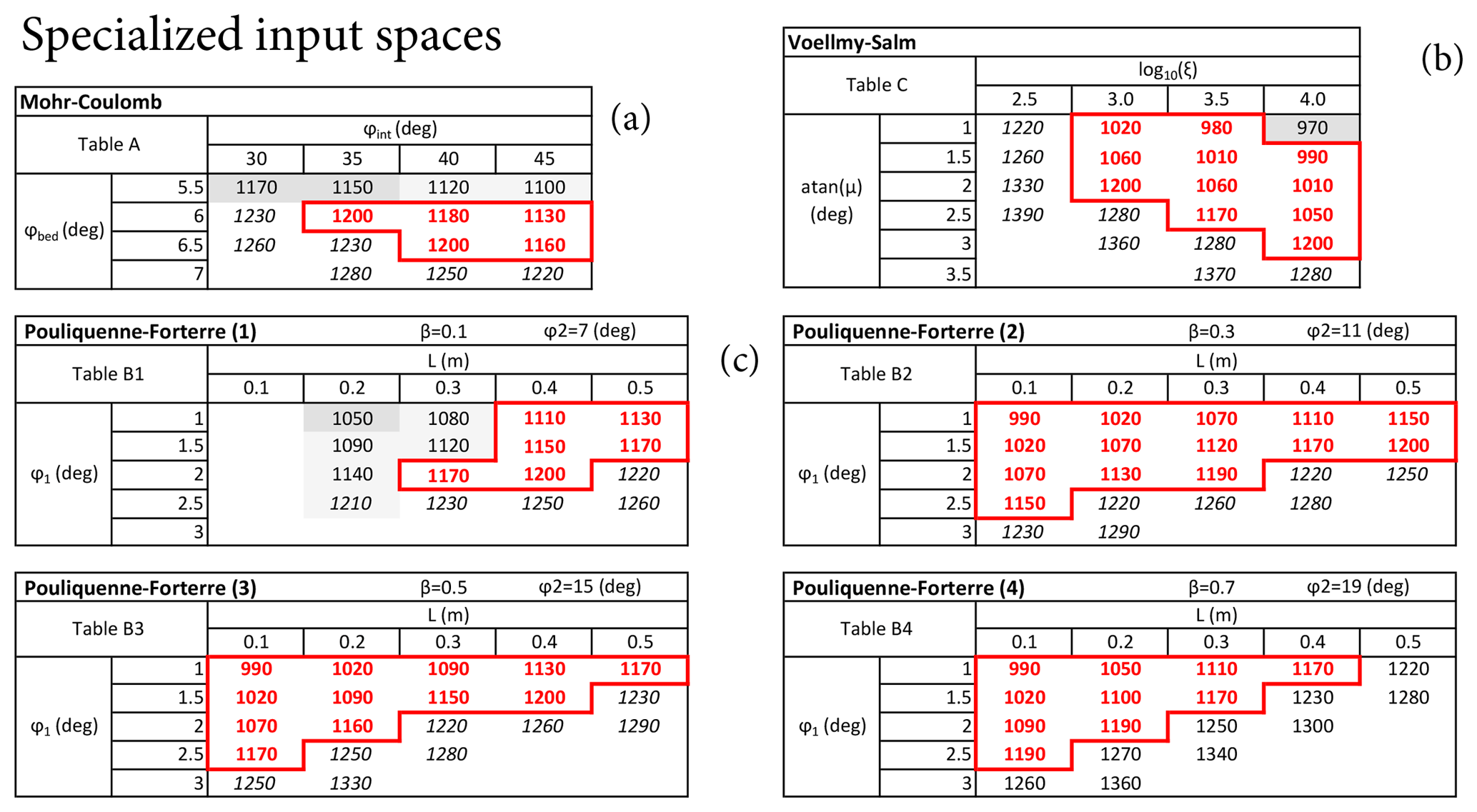
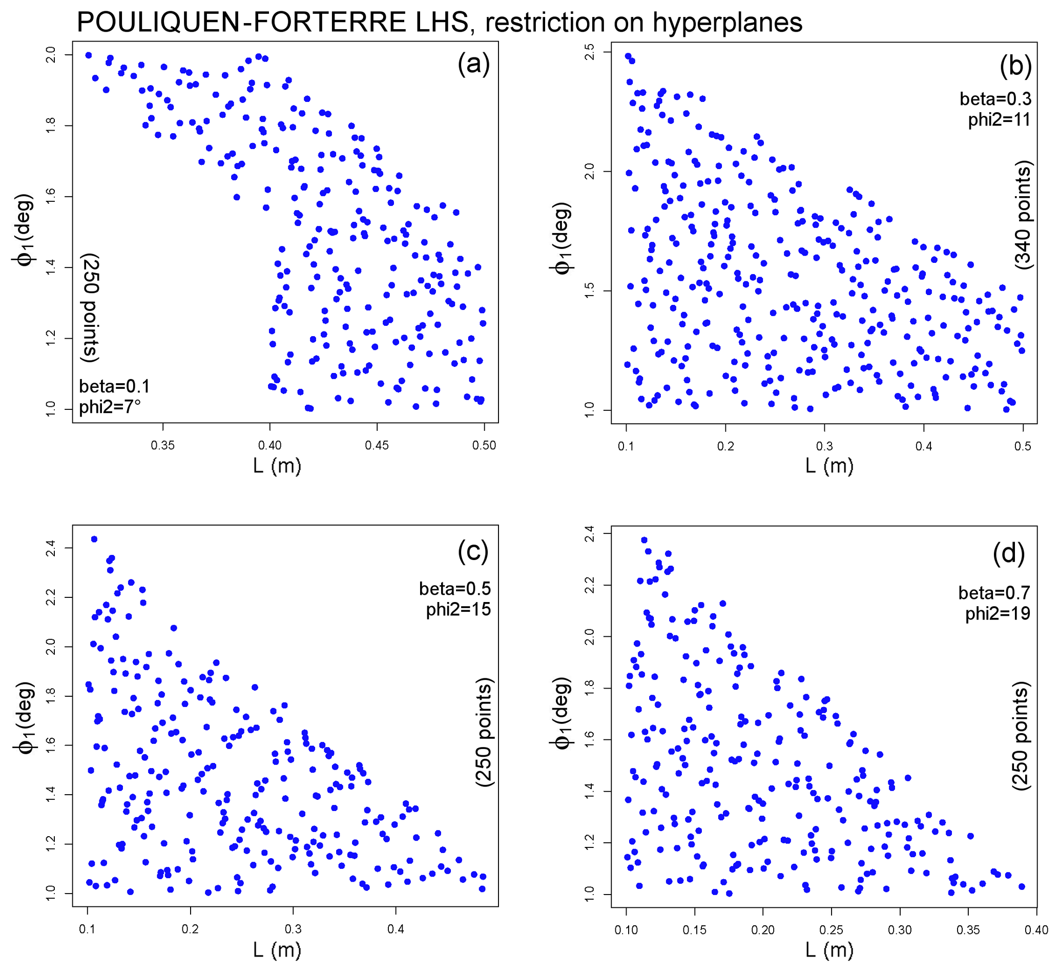
Figure 3Input space exploration and testing of (a) MC, (b) VS, and (c) PF models, m3. The 3-D input space of PF is described by four 2-D subspaces. Values reported are the minimum elevation ζ reached at t=1200 s. A gray background marks those inputs that generate unphysical flow runup and overspill the ravine walls: light gray is >0.1 m, and dark gray is >1 m. Red lines mark the subdomain Ωj of flows with ζ≤1200 m and without significant overspill issues.
Figure 3 reports the minimum elevation ζ inundated at 1200 s and a summary of overspill issues. These values are generated with reference to a flow volume of m3, roughly equivalent to the mean value of our range, and so the input spaces have two dimensions in MC and VS and three in PF. Following the empirical falsification principle, we snip the input range by deleting those regions that do not satisfy our requirements. The subspaces obtained by this procedure do not have a rectangular shape but look like parallelograms – this is because the effects of the input variables on the output are not independent. Maximum flow height maps of all these tests are included in SI1–SI3 in the Supplement.
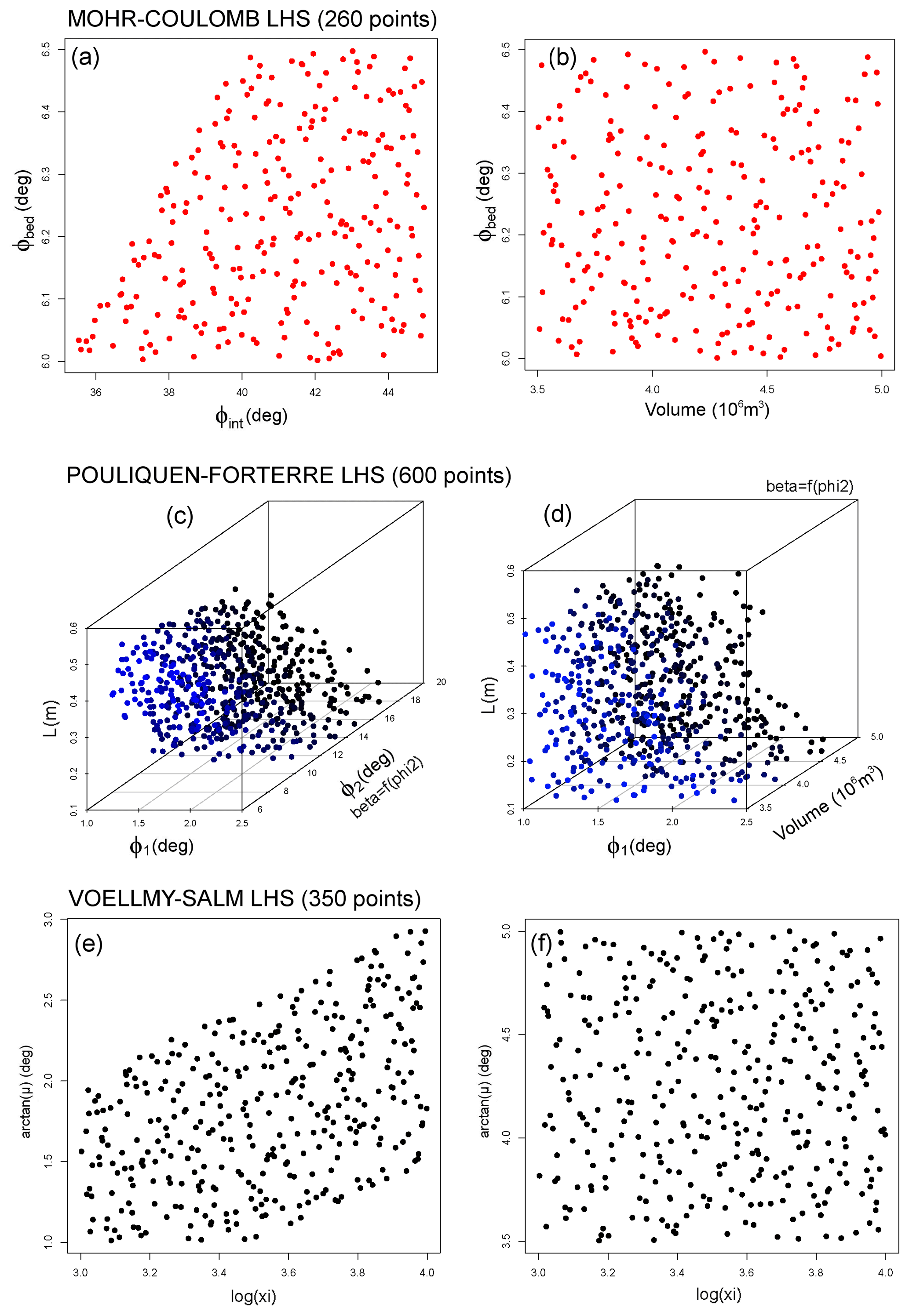
Figure 4Overview of the specialized experimental design in (a, b) MC, (c, d) PF, and (e, f) VS models. Panels (a, c, e) are projected along the V coordinate, and (b, d, f) are projected the along ϕint, ϕ2, and ξ coordinates. In (c, d), the color expresses the distance along the third dimension.
-
In MC we observe overspill issues if ϕbed<6∘ and a runout that is too short if ϕbed>6.5∘. We also note an increase in the runout distance as ϕint increases. In particular, ϕint≥35∘ is required to inundate the village.
-
In VS the overspill is observed in the region . In contrast, the region produces runouts that are too short.
-
Model PF must be treated with greater care because of its higher dimensionality. We divide its behavior along four different hyperplanes, corresponding to different values of ϕ2 and β=f(ϕ2). Overspill was observed only in the hyperslice with ϕ2=7∘ and L<0.4 m. In general, ϕ1<3∘ is required to have a long enough runout.
3.2 Probability measures and specialized experimental design
Initially, ∀j, we uniformly distribute the measure supported in the general input space :
where (, …, ) is the parameterization of model Mj∈ℳ described above, and ∀k, (, ) is the input range. Latin hypercube sampling is performed over [0, 1].
We enhance the sampling procedure by relying on orthogonal arrays (Owen, 1992a; Tang, 1993; Patra et al., 2018b). Those dimensionless samples are thus linearly mapped over the required intervals, providing the general experimental design. Then, according to the definition of the specialized input space, we remove the design points which lie outside of the boundary.
Figure 4 displays the plot of this specialized experimental design. In PF, the design is embedded in ℝ4, and in Fig. 5 we show the plot of ancillary experimental designs supported over the four hyperplanes described in Fig. 3, corresponding to different values of ϕ2 and β=f(ϕ2). In the following, our time domain is s], which provides sufficient time for simulated flows to realistically inundate the village, considering the inputs in Ωj. We call tf=2400 s the ending time of the simulation.
Figure 6 summarizes all the steps of our approach, following the notation defined in the Introduction. We remark that the comparison of observed data to the statistical summary of the outputs can provide some information on possibly untested plausible flows and on the hypothetical necessity of implementing additional models.

Figure 6Diagram of the steps of our meta-modeling approach. Our statistical summary includes the local analysis of contributing variables.
We devise multiple statistical measures for analyzing the data according to the specialized LHS design described in the previous section. In general, for each Mj∈ℳ, we sample the model inputs in a Monte Carlo simulation, and the output of each sample run is calculated as a function fj(ω, , t), where ω is the input, t is the time and is a spatial element of the computational grid. The family of these functions naturally defines a random variable which expresses the model outputs with respect to the probability distribution Pj over the input space Ωj. This analysis generates a tremendous volume of data that we analyze using statistical methods. The results are summarized by a family of spatial maps and temporal graphs, displaying the expectation of the model outputs and also their 5th and 95th percentiles, with respect to Pj.
In particular, we select five sites and we gather detailed results from our simulations in those special locations. These are called sites 1–5 (stars in Fig. 1). They all belong to the set of the 60 sections studied in Saucedo et al. (2008), and the corresponding section numbers are also reported. In detail they are as follows:
-
Site 1, section 23, UTM 656690.1∘ N, 2160985.4∘ E is along the main ravine ∼6 km upstream from the Atenquique village.
-
Site 2, section 28, UTM 660380.8∘ N, 2162530.8∘ E is in Arroyo Seco tributary, ∼2.5 km upstream from the confluence.
These first two are not described in detail, but the related results are included in SI4–SI5 in the Supplement. Conversely, we focus our analysis on the other three points, all placed along the main ravine in proximity to Atenquique village.
-
Site 3, section 21, UTM 660258.1∘ N, 2161315.2∘ E is ∼2 km upstream from the village.
-
Site 4, section 17, UTM 662453.1∘ N, 2160360.1∘ E is immediately upstream from the village, close to the confluence with Arroyo Seco and Arroyo Plátanos tributaries.
-
Site 5, section 42, UTM 663539.0∘ N, 2160200.0∘ E. In the village, ∼1 km downstream from the previous site.
We note that close to Site 4 there are the supports of the new bridge of the freeway to the city of Colima. Results related to Site 5 are displayed in SI6 in the Supplement, but local flow height and speed will be further analyzed in the following sections.
4.1 Percentile maps of maximum flow depth and kinetic energy
First of all, we report the spatial maps of maximum flow depth, h, and kinetic energy, κ:
In our depth-averaged approach the kinetic energy4 is defined as
where and are the components of momentum in the x and y directions.
This is equivalent to , : that is, half the flow height times the speed square. Thus, κ is formally the kinetic energy density per unit of surface area, for a mass with unit density.
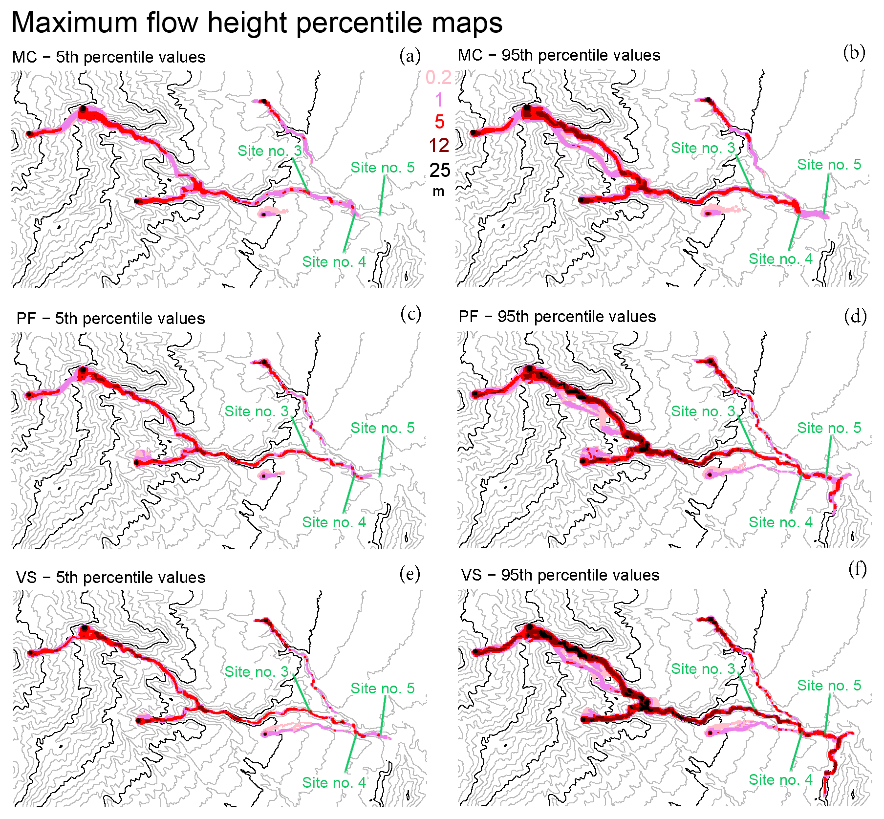
Figure 7Maximum flow height H as a function of time in (a, b) MC, (c, d) PF, and (e, f) VS models. Panels (a, c, e) are the 5th and (b, d, f) are the 95th percentile values with respect to Pj. Colors are related to the flow height. Elevation contours are included at intervals of 100 m (gray) and 500 m (black) (NASA – JPL, 2014). Sites 3–5 are displayed.
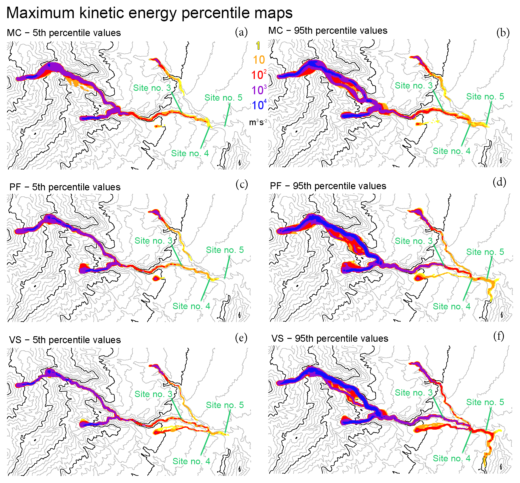
Figure 8Maximum kinetic energy K as a function of time in (a, b) MC, (c, d) PF, and (e, f) VS models. Panels (a, c, e) are the 5th and (b, d, f) are the 95th percentile values with respect to Pj. Colors are related to the energy in logarithmic scale. Elevation contours are included at intervals of 100 m (gray) and 500 m (black) (NASA – JPL, 2014). Sites 3–5 are displayed.
The kinetic energy, K, in a traditional sense may be calculated over an arbitrary region R as follows:
where ρ is the density of the flow, typically in [1000, 2000] kg m−3, depending on the flow water content.
Figure 7 reports the maximum flow depth, H, and Fig. 8 reports the maximum kinetic energy, K. MC shows the lowest values of both flow depth and energy, while VS shows the highest, especially in the distal part of the domain. In MC, the flow in the tributaries is not capable of reaching the village, while in the 95th percentile maps of PF and VS, it is. In VS, the flow in Arroyo Plátanos joins the main ravine, even in the 5th percentile map. In general, local maxima of flow depth are located in the ravine, while the kinetic energy shows a more regular decrease. The energy values at the head of the flow are in [1, 10] m3 s−2, which is a relatively slow flow compared to the dynamics observed upstream. Significant overspill issues are absent, but in the 95th percentile maps all the models report some flow in the Dos Volcanes ravine, of about [1, 5] m at maximum height, and slightly less in PF.
4.2 Local properties of the flow
We further analyze the flow properties at two of the sites selected above, which are located in the distal part of the flow (sites 3 and 4), with very different results. All the quantities reported are estimated on the element of the grid, which contains the coordinates of the site. We remark that the grid is adaptive, and hence the values can be affected by the size and position of the element. However, the integration over the input space significantly reduces this effect (Patra et al., 2018b).
Along with the locally analyzed flow height and speed, we calculate the local contributing variables in the modeling equations: that is, the dominance factors and the expected contributions related to the force terms in the conservation laws that characterize the models. In particular, , …, N is the dominance factor and pn, is the probability that the related force term, Fn, is largest. The no-flow probability, p0, is also included, and . In contrast, ∀n, the expected contribution is the mean of the force term, Fn, divided by the greatest (dominant) term. It belongs to [0, 1] and represents the degree of relevance of the nth term with respect to the dominant one. Contributing variables and their statistics are introduced in Patra et al. (2018b) and detailed in Appendix B.
The higher dimensionality of ΩPF requires additional testing. In particular, flow height and speed are estimated on the hyperplane β=0.5, ϕ2=15∘, and the probability distributions are not remarkably different. Additional plots concerning sites 1, 2, and 5 are included in SI4–SI6 in the Supplement.
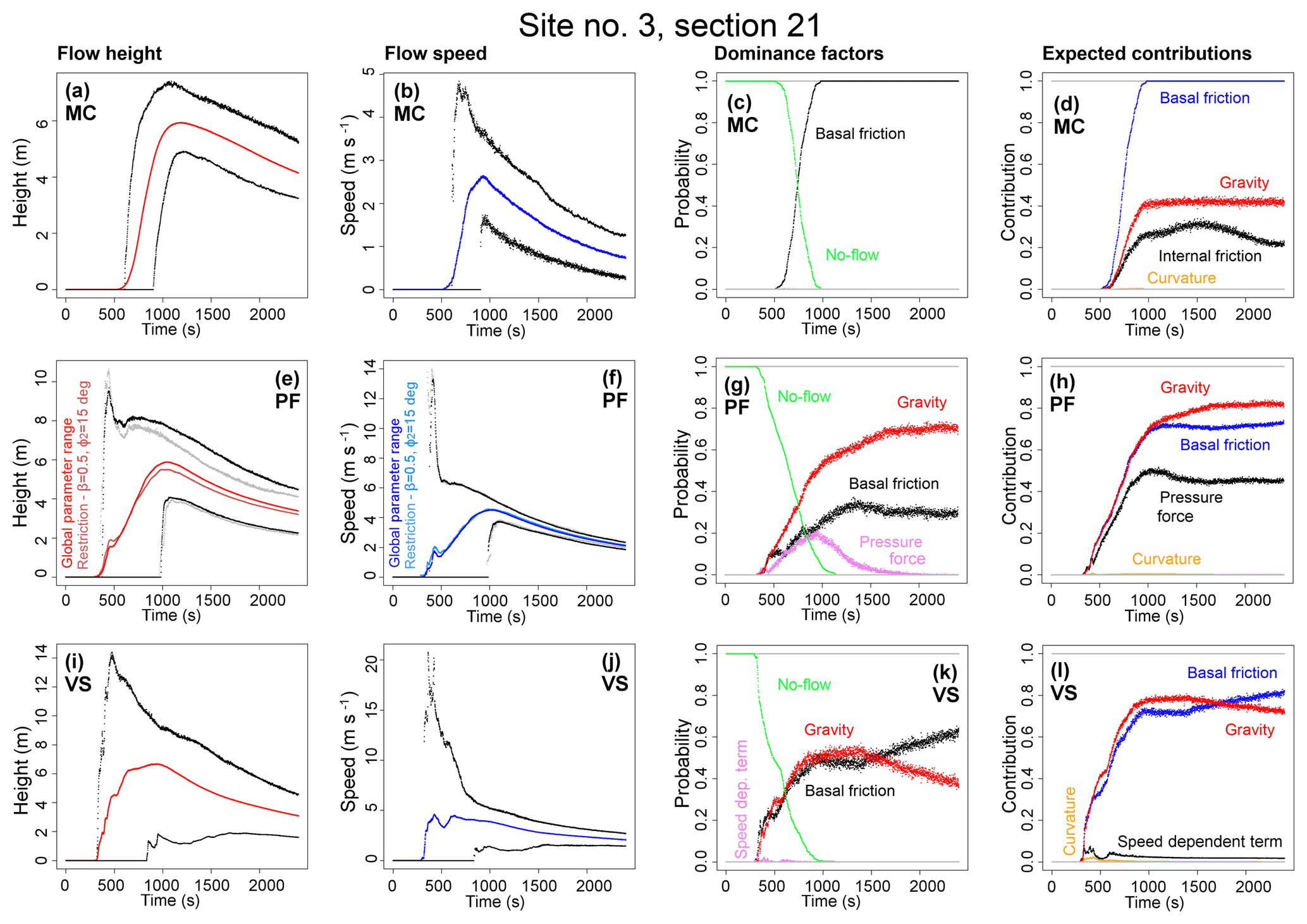
Figure 9Local flow properties at Site 3, ∼2 km upstream from Atenquique village. Panels (a, e, i) show flow height, (b, f, j) flow speed, (c, g, k) dominance factors, (d, h, l) and expected contributions of the force terms. Different models are plotted separately: (a–d) assume MC, (e–h) assume PF, and (e, f) include estimates on a hyperplanar restriction of the input domain; (i–l) assume VS. In (a, b, e, f, i, j), the colored line is the mean value, and black and gray lines are the 5th and 95th percentile bounds.
Figure 9 shows the local properties at site 3, located ∼2 km upstream from Atenquique village. In MC, the flow reaches the site in [600, 900] s, with a flow height of initially [5, 7] and [3, 5] m at tf=2400 s. Flow speed is initially in [1.5, 4.5] m s−1, and one-third of these values are at tf. Only the basal friction can be dominant, with gravitational force at 40 % and internal friction 25 %, on average. In PF the flow reaches the site at [300, 1000] s, with an initial flow height of [4, 8] m, having a short-lasting peak of 10 m in the 95th percentile and [3, 5] m at tf. Flow speed is initially in [4, 6] m s−1 and has a short peak of almost 14 m s−1 in the 95th percentile. It becomes [2.0, 2.5] m s−1 at tf. Either basal friction, gravity, or pressure force (related to the gradient of thickness) can be dominant. Gravitational force adds 80 % of the expected contribution, while basal friction adds 70 % and pressure force adds 45 %. In VS, the flow first reaches the site in [300, 800] s, with a flow height of [1.5, 12] m, initially, and a short peak at 14 m, becoming [1.5, 5] at tf. Flow speed is in [1, 15] m s−1, initially, has a short peak at 20 m s−1 and then becomes [1.5, 3.5] m s−1 at tf. Either basal friction or gravity can be dominant, both with 75 % of the expected contribution. We note that gravity tends to slightly decrease in expected contribution, as well as its dominance factor, through time. This is a numerical effect related to the variation of the mesh, which changes our approximation of local slope.
In summary, MC is characterized by a lower speed and by the dominance of basal friction. The expected contribution of the internal friction is not negligible, meaning the internal shear of the material is important. In PF, the pressure force contribution is significant, and it can even be the dominant force initially. This is related to the steepening of the flow front. An initial short-lasting wave of high speed is observed in either PF or VS, as is particularly evident in the upper bound of the plots. This fast wave is related to the closest source, 3. The uncertainty affecting height and speed is generally higher in VS than in PF, in spite of the higher dimensionality of the second.
Figure 10 shows the local properties at site 4, located immediately upstream from Atenquique village and close to the supports of the new bridge of the freeway to the city of Colima. In MC, the flow reaches the site in [1300, 2100] s, with a flow height of [2, 5.5] m. Flow speed is <0.6, and 0.1 m s−1, on average. Only basal friction is dominant, with the gravitational force being 30 % of basal friction, and 10 % of internal friction on average. In PF, the flow reaches the site at [600, 1800] s, with a flow height of [3, 6] m, which is stable in time. Flow speed is initially in [1, 4] m s−1 and half of these values are at tf. Either basal friction or gravity can be dominant. Gravitational force can be 95 % of the expected contribution, while basal friction is 65 % and the pressure force is 25 %.
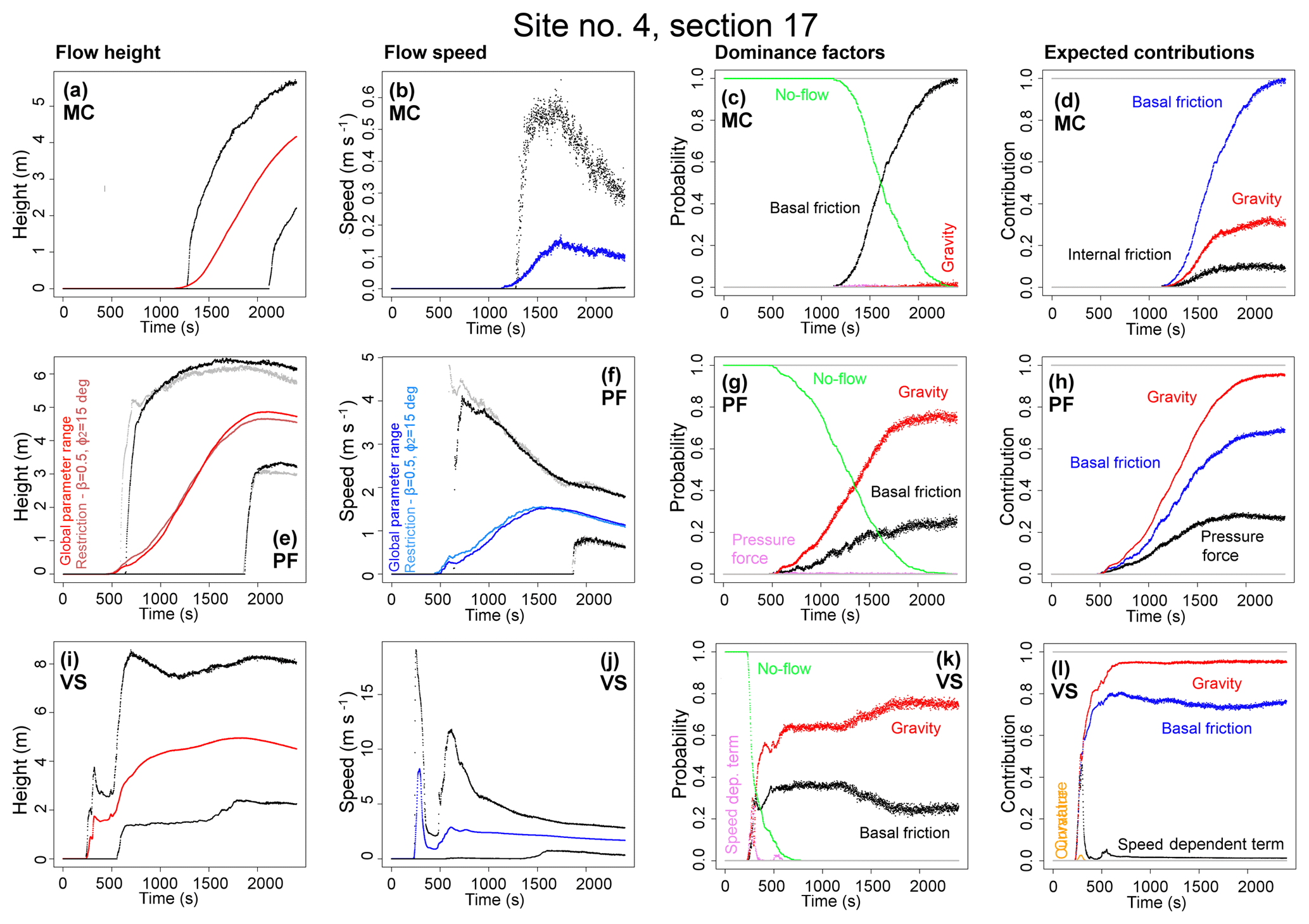
Figure 10Local flow properties at Site 4, immediately before Atenquique village. Panels (a, e, i) show flow height, (b, f, j) flow speed, (c, g, k) dominance factors, and (d, h, l) expected contributions of the force terms. Different models are plotted separately: (a–d) assume MC, (e–h) assume PF, and (e, f) include estimates on a hyperplanar restriction of the input domain; (i–l) assume VS. In (a, b, e, f, i, j) colored line is mean value, and black and gray lines are 5th and 95th percentile bounds.
In VS, the flow reaches the site in [250, 550] s, with a first wave of <3 m. A second wave of [1.5, 8] m arrives and stays stable in depth. Flow speed also shows two waves – it is <19 m s−1 initially, then rises to <12 m s−1, with a gap in the middle. It is [1, 3] m s−1 at tf. Either gravity or basal friction can be dominant, with 95 % and 80 % of the expected contribution, respectively. In the initial fast wave, the speed-dependent friction can be dominant, with 25 % of the expected contribution.
In summary, all the models show lower flow height and speed than at the previous site upstream. The flow depth is stable, without decreasing downstream, meaning no formation of a significant deposit. MC is much slower than the other models, and its dynamics is completely dominated by basal friction. An initial, short-lasting wave of high speed is observed in VS. This fast wave is related to source 5 in Arroyo Platános.
In Site 5, reported in SI6 in the Supplement, all the models show a further decrease in flow height and speed compared to the previous site. In MC, the site is not always reached, and in PF some input values inundate the site only at the end of the time domain.
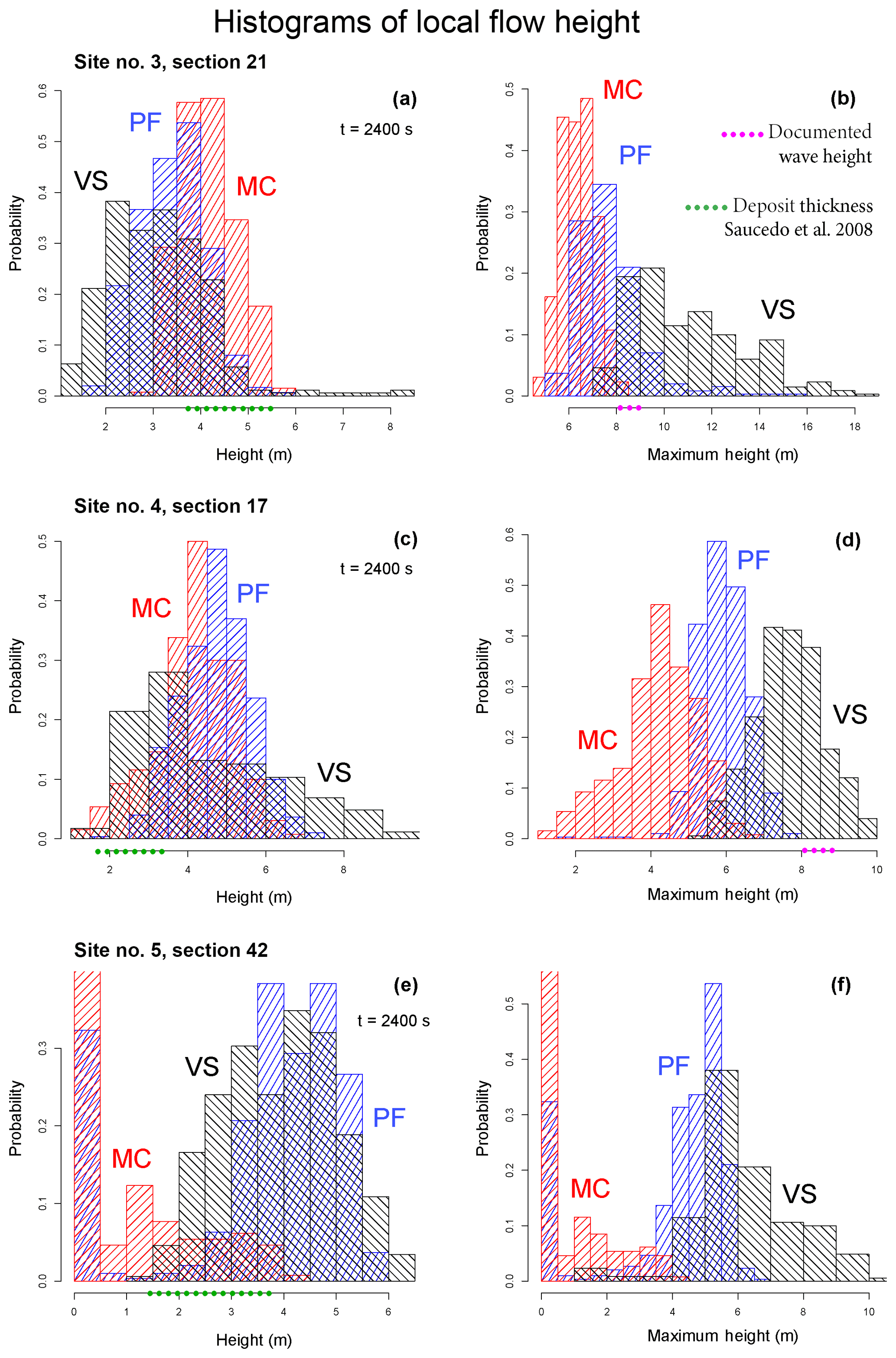
Figure 11Histograms of local flow height in sites 3–5. Panels (a, c, e) show height at t=2400 s, while (b, d, f) show maximum height. Different models are displayed with different colors. Dots on the height axis show the uncertainty interval of data: green is the deposit thickness of Saucedo et al. (2008) and unpublished data; violet is the wave height documented by the survivors.
Figures 11 and 12 show the flow height and speed histograms at the three selected sites, with either their maximum value or their value at t=2400 s. These confirm what is summarized in the previous section. The following probability density values are evaluated with respect to m and m s−1. In Fig. 11 the following is shown:
-
At Site 3, flow height pdf at tf is above 0.1 over [3, 5.5] m in MC, [2, 4.5] m in PF, and [1.5, 4.5] m in VS. The first two models are more peaked, while the third produces a tail of very large thickness values, up to 8 m. The maximum height pdf is above 0.1 over [5.5, 8] m in MC, [6, 9] m in PF, and [8, 13] in VS.
-
At Site 4, flow height pdf at tf is above 0.1 over [2.5, 6] m in MC, [3, 6] m in PF, and [2, 7] m in VS. The maximum height pdf is above 0.1 over [2.25, 6] m in MC, [5, 7] m in PF, and [6, 9.5] m in VS. The three models show clearly separate modal values at 4, 6, and 8 m, respectively.
-
At Site 5, MC and PF do not always reach the site in s, so they both show a modal value of flow height at 0 m. The flow height pdf at tf is above 0.1 over [1, 1.5] m in MC with a tail up to 3.5 m, [3, 5.5] m in F, and [2, 6] m in VS. The maximum height pdf is almost equal to final height in MC, and it is above 0.1 over [3.5, 6] m in PF and [3.5, 9] m in VS. Both PF and VS show a modal value at 5 m.
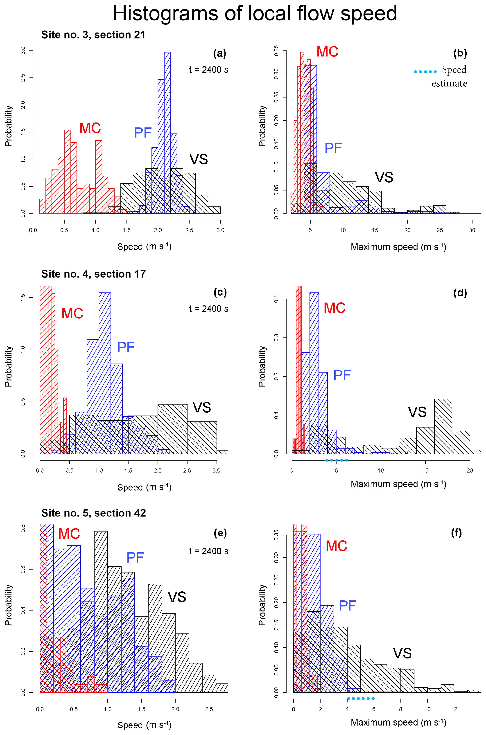
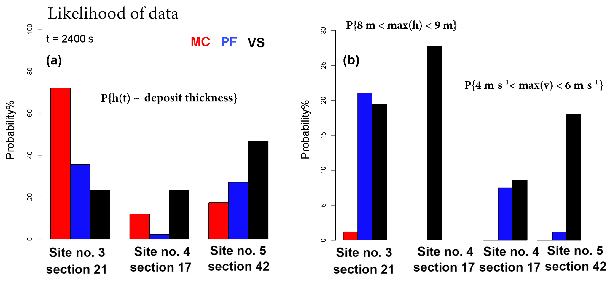
Figure 13Bar plots of data likelihood in sites 3–5. Panel (a) compares flow height at t=2400 s with observed deposit thickness (Saucedo et al., 2008). Panel (b) compares maximum height and maximum speed with observed wave height (Ponce-Segura, 1983) and the peak flow speed obtained using the methods of Pierson (1985). Different models are displayed with different colors.
In Fig. 12 the following is shown:
-
At Site 3, flow speed pdf at tf is above 0.25 over [0.1, 1.4] m s−1 in MC, [1.6, 2.4] m s−1 in PF and [1.4, 2.8] m s−1 in VS. MC is bimodal at 0.5 and 1 m s−1, while PF has a modal value at 2.1 m s−1. The maximum speed pdf is above 0.05 over [1, 7] m s−1 in MC, [4, 8] m in PF, and [4, 16] in VS. PF and VS have tails up to 25–30 m s−1.
-
At Site 4, flow speed pdf at tf is above 0.25 over [0.00, 0.45] m s−1 in MC, [0.6, 1.8] m s−1 in PF, and [0.5, 3.0] m s−1 in VS. PF has a modal value at 1 m/s. Maximum speed pdf in MC is concentrated below 1 m s−1. In PF, it is above 0.25 over [1, 5] m s−1. In VS, it is bimodal and above 0.25 over [2, 6] and [12, 20] m s−1.
-
At Site 5, flow speed pdf at tf is above 0.25 over [0.0, 0.4] m s−1 in MC, [0.0, 1.4] m s−1 in PF, and over [0.0, 0.2] and [0.4, 2.2] m s−1 in S. The maximum speed pdf is above 0.05, over [0.0, 0.2] and [0.4, 1.2] m s−1 in MC, [0, 4] m in PF and [0, 9] in VS. PF and VS have tails up to 8 and 13 m s−1, respectively.
5.1 Alternative performance scores of the models
In Figs. 11 and 12, we display the empirical data concerning the observed quantities. These intervals are examples of uncertain data utilized to test our methodology. Further research could refine or modify them. Unfortunately, the speed of the 1955 Atenquique flow is unknown. In our analysis, we consider the peak speed estimated using the superelevation method of Pierson (1985), as already reported in Saucedo et al. (2008). We remark that, although the reconstruction of hydrographs from an analogous flow may provide us with time-dependent data, this would introduce additional uncertainty that is difficult to constrain.
Our empirical data include the following:
-
The deposit thickness, calculated from the envelope of the closest field sections, is [3.7, 5.5] m at Site 3, [1.7, 3] m at Site 4, and [1.4, 3.8] m at Site 5 (Saucedo et al., 2008).
-
The flow height in Atenquique village, from historical documents and witnesses, is [8, 9] m at Site 3 and/or Site 4 (Ponce-Segura, 1983; Saucedo et al., 2008).
-
The peak flow speed following the inundation of the village, based on the superelevation method, is [4, 6] m s−1 at Site 4 and/or Site 5 (Pierson, 1985; Saucedo et al., 2008).
The estimation of the likelihood of the pieces of observed data is an essential step towards the definition of partial solutions of the inverse problem. Besides this, it is also relevant information in the model selection problem. The likelihood of a data piece, Di, attaining its value given a certain model is defined as Pj(Di), , . We remark that this is not a pdf value, but the probability of a measurable set. Figure 13 shows the bar plots of data likelihood. Figure 13a considers deposit thickness values under the assumption that they are equivalent to the flow height at tf. At Site 3, 70 % of MC inputs provide flow thickness consistent with the deposit range, against 35 % of PF and 20 % of VS inputs. At Site 4, likelihood scores are lower: 20 % in MC, 10 % in VS, and <5 % in PF. At Site 5, instead, we have 15 % in MC, 25 % in PF, and 45 % in VS. Figure 13b evaluates the maximum flow height when the flow entered Atenquique village. In Site 3, 20 % of inputs in PF and VS provide results consistent with data, while only <5 % do so in MC. At Site 4, the likelihood score of VS is 27 %, while it is null in the other models. Figure 13c focuses on the maximum flow speed after the flow inundated the village. At Site 4, 8 % of inputs in PF and 9 % in VS provide speeds in the most likely range. At Site 5, these are only 1 % in PF and 17 % in VS.
In summary, model performance is dependent on the selected quantity of interest and on the spatial location. Regarding the deposits, MC performs well at Site 3, while VS does so at Site 5. In the evaluation of the maximum flow depth in the village, both PF and VS can replicate the values at Site 3, and only VS can replicate the values at Site 4. If we focus on the maximum flow speed, at Site 4 both PF and VS perform moderately well, while at Site 5, only VS can provide speed values inside the assumed range.
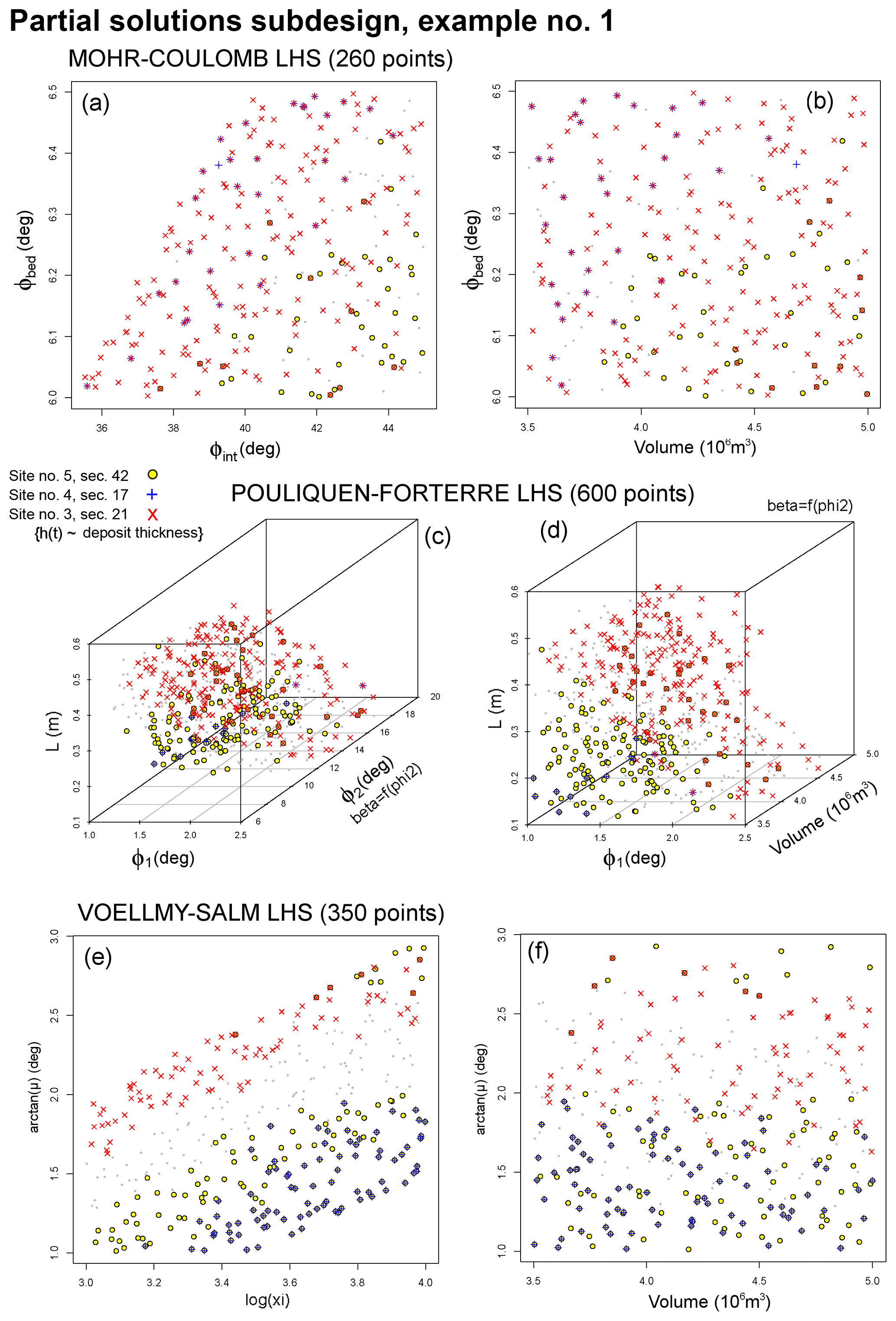
Figure 14Example 1 of partial solution inputs in (a, b) MC, (c, d) PF, and (e, f) VS experimental design. Panels (a, c, e) are projected along the V coordinate, and (b, d, f) are projected along ϕint, ϕ2 and ξ coordinates. The color expresses the considered data: yellow is deposit thickness at Site 5, blue at Site 4, and red at Site 3 (Saucedo et al., 2008).
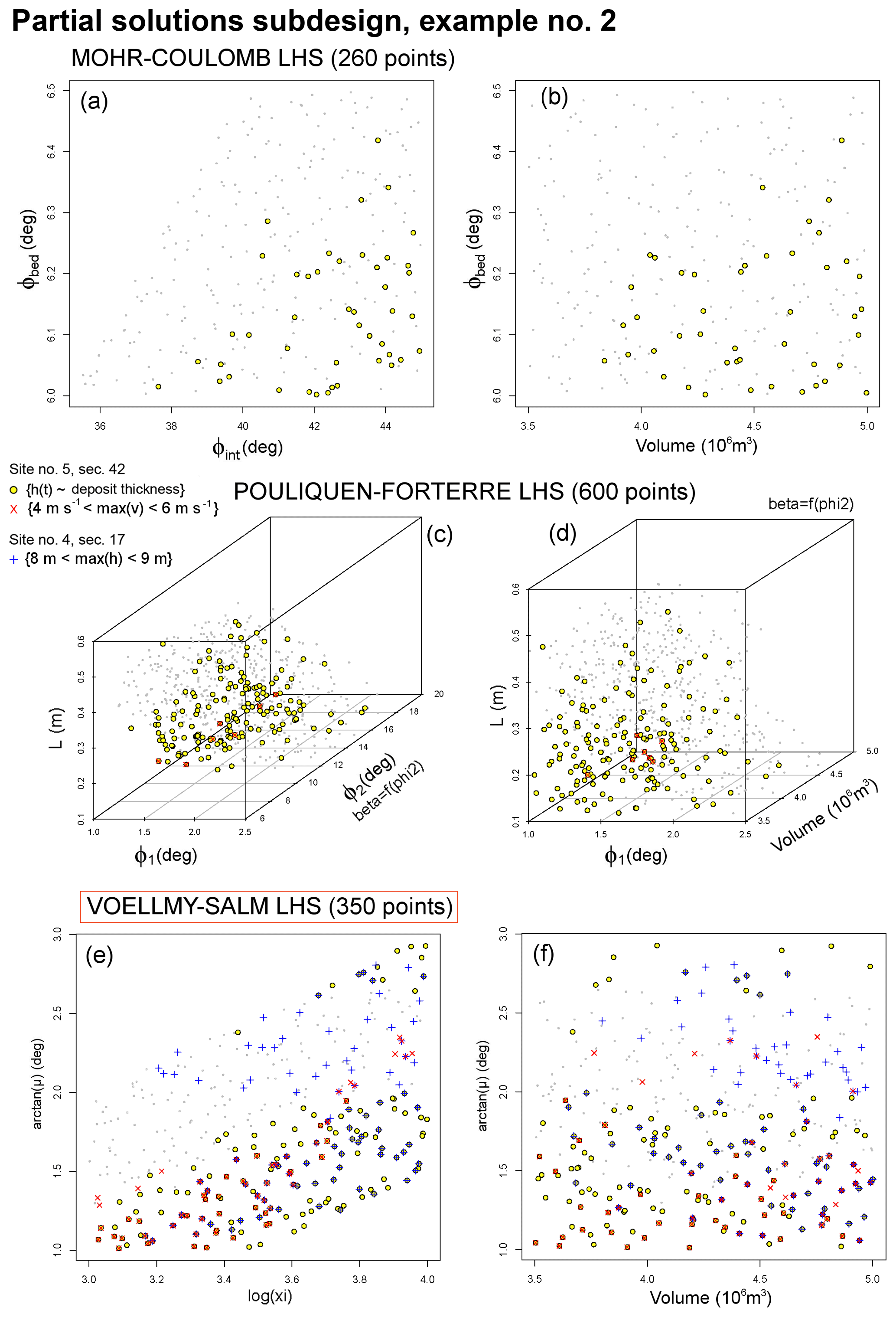
Figure 15Example 2 of partial solution inputs in the (a, b) MC, (c, d) PF, and (e, f) VS experimental designs. Panels (a, c, e) are projected along the V coordinate and (b, d, f) are projected along ϕint, ϕ2, and ξ coordinates. The color expresses the considered data: yellow is deposit thickness at Site 5 (Saucedo et al., 2008), blue is wave height at Site 4 (Ponce-Segura, 1983), and red is peak flow speed at Site 5 (Pierson, 1985).
Figures 14–16 display three examples of partial solutions in the specialized experimental design. For each example of n=1, 2, 3 we select a subfamily of empirical data and define, ∀j,
Example 1 focuses on the deposit thickness data at sites 3–5. Examples 2 and 3 consider the deposit thickness at Site 5 only. Additionally, Example 2 evaluates the maximum flow height at Site 4 and the maximum flow speed at Site 5, while Example 3 does that at Site 3 and Site 4, respectively.
Figure 14 concerns Example 1. In all the models, . In MC, the set of inputs that replicate the deposit thickness at Site 4 are disjoint from those at Site 5. Instead, in PF and VS the inputs related to Site 3 are disjoint from those related to Site 4. Figure 15 concerns Example 2. In MC and PF, the maximum flow height from the data is never reproduced. In MC, the required maximum flow speed is never achieved. Thus, only if j=VS.
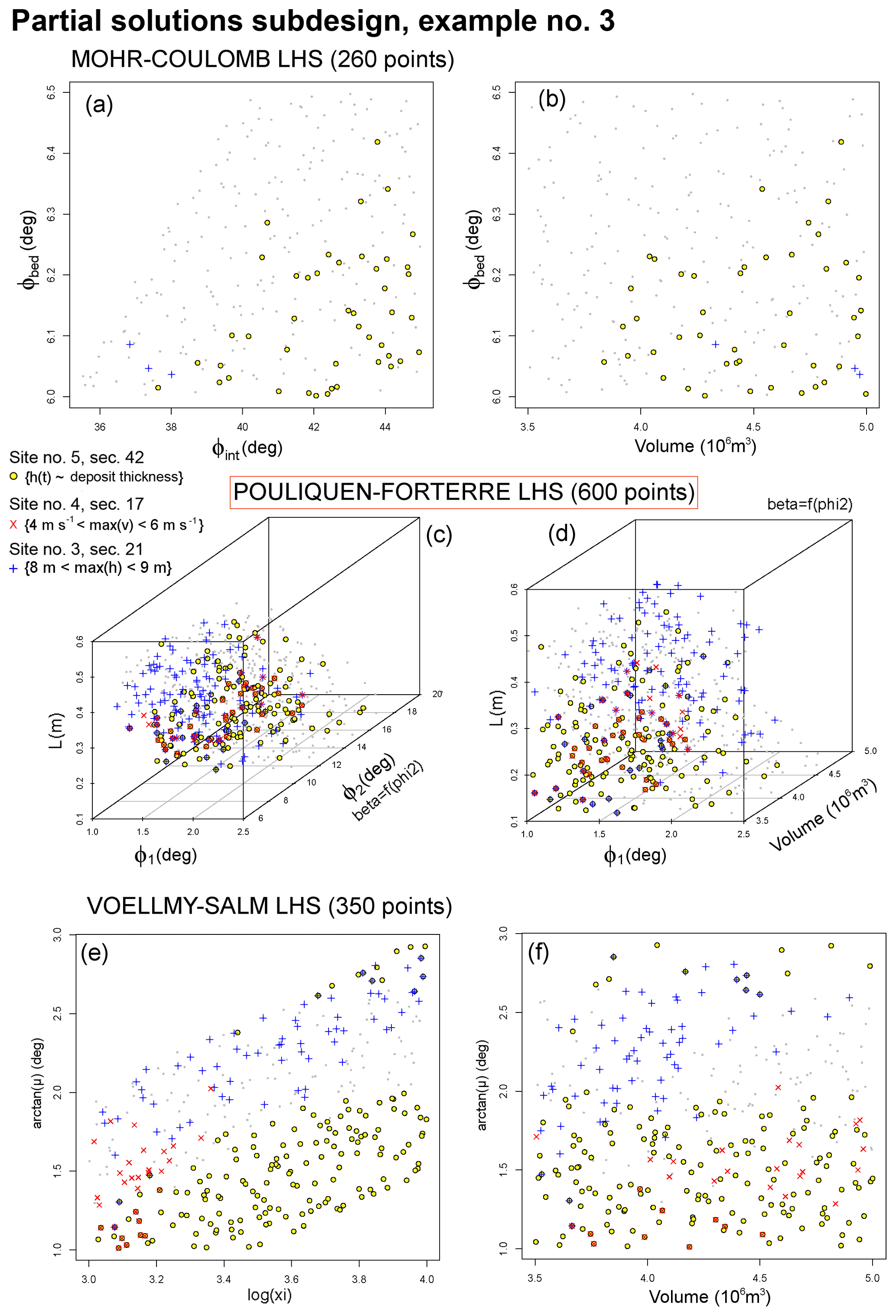
Figure 16Example 3 of partial solution inputs in the (a, b) MC, (c, d) PF, and (e, f) VS experimental designs. Panels (a, c, e) are projected along the V coordinate, and (b, d, f) are projected along ϕint, ϕ2, and ξ coordinates. The color expresses the considered data: yellow is deposit thickness at Site 5 (Saucedo et al., 2008), blue is wave height at Site 3 (Ponce-Segura, 1983), and red is peak flow speed at Site 4 (Pierson, 1985).
The partial solution inputs in are bounded by
Figure 16 is related to Example 3. In MC, the required maximum flow speed from the data is never reproduced. We have that for . In PF, the partial solution inputs in are bounded by
In VS, only one point belongs to the partial solution input set, with arctan (μ)≃1.2, ξ≃3.1, m3. Remarkably, the input spaces reproducing the three required pieces of empirical data are almost disjoint in pairs, and is small and close to the frontiers of the uncertainty ranges. Additional details in PF over the hyperplane {β=0.5, ϕ2=15} described in Fig. 3 are included in SI7 in the Supplement.
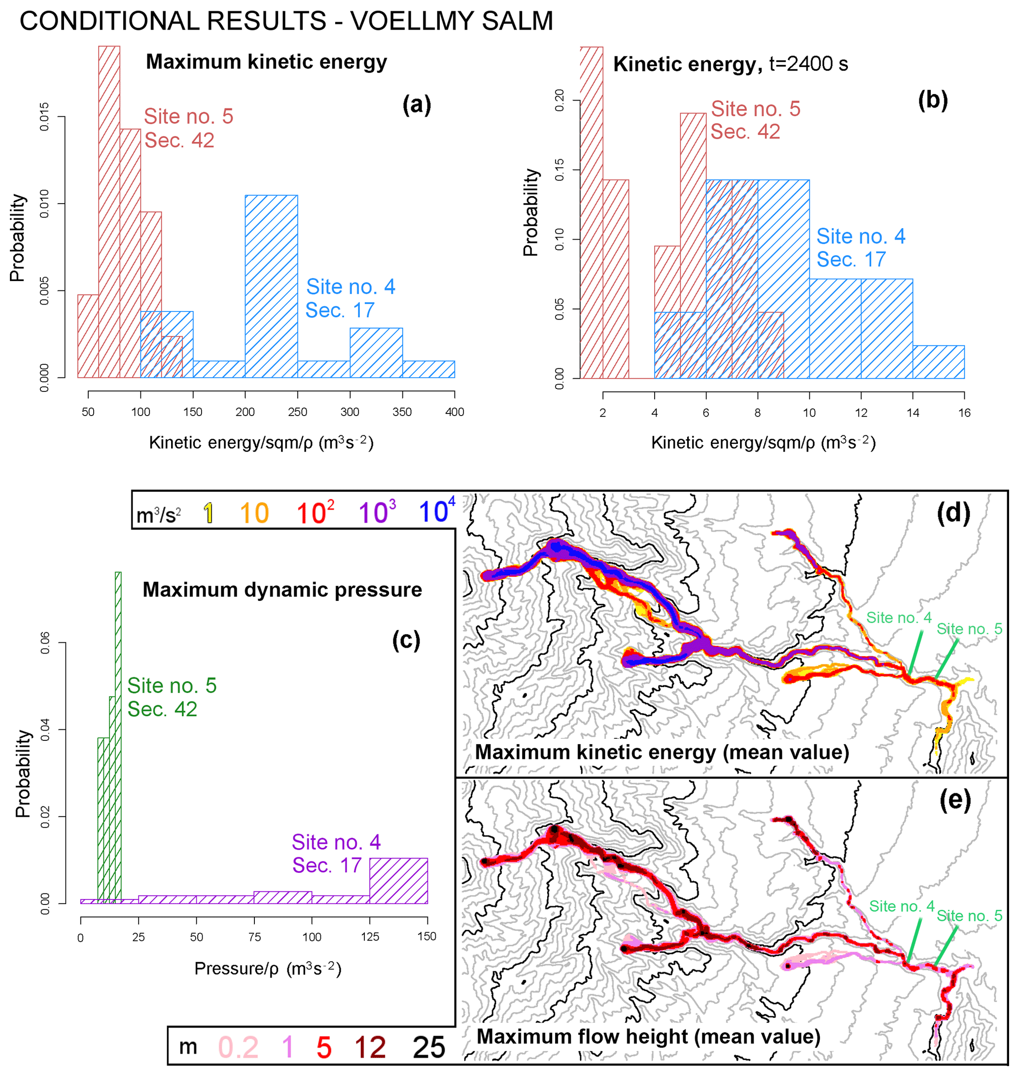
Figure 17Flow properties of the VS model, over the input space . Histograms of (a, b) local kinetic energy and (c) dynamic pressure at sites 4 and 5, (a) at t=2400 s and with (b, c) maximum value. Different sites are displayed with different colors. Mean values over of the maps of maximum (d) kinetic energy and (e) flow height as a function of time. Colors are related to their values. Elevation contours are included at intervals of 100 m (gray) and 500 m (black) (NASA – JPL, 2014). Sites 4 and 5 are displayed.
6.1 Examples of conditional results
The solution of the partial inverse problems can enable us to select a model, which nevertheless depends on the required properties and the spatial location.
-
In Example 1 the partial inverse problem is not well posed.
-
In Example 2 only in VS can we find solutions .
-
In Example 3 both in PF and VS we find solutions . .
The points in the experimental design that belong to and are 21 and 9 respectively. We do not detail because it contains only one design point and the results can be disrupted even by relatively small variations of the inputs. Additional tests at a finer resolution in the experimental design could be performed to achieve a more accurate characterization of the conditional input spaces if required.
In Figs. 17 and 18, we report the histograms of
at sites 4 and 5. The spatial maps of the maximum in flow height, h, and kinetic energy, κ, are also displayed. The dynamic pressure Q and the kinetic energy κ formally assume a mass with unit density.
In Fig. 17, at Site 4,
and at Site 5,
The modal values of K are ∼225 and 60 m3 s−2.

Figure 18Flow properties of PF model, over the input space . Histograms of (a, b) local kinetic energy and (c) dynamic pressure at sites 4 and 5, (a) at t=2400 s and with (b, c) maximum value. Different sites are displayed with different colors. Mean values over of the maps of maximum (d) kinetic energy and (e) flow height as a function of time. Colors are related to their values. Elevation contours are included at intervals of 100 m (gray) and 500 m (black) (NASA – JPL, 2014). Sites 4 and 5 are displayed.
In Fig. 18, at Site 4,
and at Site 5,
Modal values are not well-constrained in this case.
In the spatial maps, PF shows slightly lower maximum flow height and significantly lower energy than VS, especially in the distal part of the domain. The flow in the tributaries can reach the village, except for the smallest flows of Arroyo Plátanos in PF, which, however, at tf are only tens of meters from the main branch. As in the unconditional maps, local maxima of flow height are located in the ravine, while the kinetic energy shows a more regular decrease.
In summary, the statistical analysis of the partial solutions told us the following:
-
The deposit thickness is the three selected sites is not reproduced by any of the models. In particular, the input choices that fit Site 3 are inconsistent with those that fit the deposit downstream. This advocates the possibility of testing additional models, for example including an entrainment term in the mass conservation equation.
-
The MC model is not capable of reproducing the required maximum flow height and speed in the village. Its feasible input space does not allow us to reduce the friction further. Even if PF can reproduce the required height and speed when impacting the village, only VS is also capable of maintaining those values in the downstream part of the village.
In particular, models using MC-based rheologies are unlikely to reproduce the properties of the 1955 flow. Instead, the flexible basal friction angle in PF allows for both higher speed and longer runout, consistent with those observed. The higher dimensionality of its parameter space does not significantly increase the uncertainty affecting the outputs. Similarly, the velocity-dependent term in VS is a very robust mechanism for preserving numerical stability, avoiding the spurious results that affect the MC model at equivalently low values of basal friction. Indeed the highest levels of simulated speed are observed with VS.
We remark that the assumed [4, 6] m s−1 constraint on the maximum flow speed has an immediate effect on the dynamic pressure estimates. Imposing it at Site 5 as in Example 2 or Site 4 as in Example 3 can radically change the results, even if the required deposit thickness at Site 5 is not modified. Additional information on the speed properties in the village could thus allow us to further discriminate the performance of the models.
In this study, we have introduced a new prediction-oriented method for hazard assessment of volcaniclastic debris flows (lahars), based on multiple geophysical mass flow models. Similar strategies have been applied in hurricane hazard analysis (Krishnamurti et al., 2016; Ghosh and Krishnamurti, 2018). In particular, our approach decomposes the original inverse problem into a hierarchy of simpler problems and allows for the exploration of the impact of synthetic flows that are similar to those that occurred in the past but different in plausible ways.
We applied our procedure to a case study of the 1955 Atenquique volcaniclastic debris flow. We adopted and compared three depth-averaged models based on the Saint Venant equations that are widely used in hazard assessment, namely Mohr–Coulomb (MC), Pouliquen–Forterre (PF), and Voellmy–Salm (VS).
-
We defined a specialized experimental design after assuming the realism of the underlying physics, the numerical simulation is robust in some sense, and the flow dynamics or inundation output is meaningful. This produced a range of output simulations that contain valuable information for hazard assessment.
Indeed, these outputs do not strictly reconstruct past flows, so can provide hazard estimates under constraints weaker than those used therein, potentially including cases of extreme events. Moreover, our designs were not trivial geometrically due to the correlated effects of model inputs. This is a first step towards the development of an objective and partially automated experimental design.
-
We described the statistics of the outputs and contributing variables by performing a Monte Carlo simulation over the specialized design. We made global maps of the flows and investigated detailed characteristics. This allowed us to calculate the likelihood that different model realizations reasonably represented the 1955 Atenquique flow, given multiple pieces of field data regarding its characteristics. Depending on how it is looked at, the exercise provided useful information in either model selection or data inversion.
Our analysis concerned the mean values and uncertainty percentiles of quantities of interest. Moreover, the probabilistic setting allowed us to make inferences regarding the uncertainty affecting the data. We analyzed the contributing variables, which shed light on the different assumptions underlying the three models. In particular, the MC model is generally characterized by a lower speed over its feasible input space, when compared to the other models. The expected contribution of the internal friction is significant, meaning the internal shear of the material is important. In the PF model, the pressure force contribution related to the steepening of the flow front was locally significant and was sometimes even the dominant force. An initial, short-lasting wave of high speed related to the closest of the multiple sources was observed in both PF and VS. The uncertainty in height and speed was generally higher in VS than in PF, in spite of the higher dimensionality of the second.
-
We constructed partial solutions to the inverse problem, conditioning the specialized experimental design to be consistent with subsets of the observed data. We described the corresponding input sets and investigated their intersection. We found model selection to be inherently linked to the inversion problem. That is, the partial inverse problems enabled us to select models depending on the example characteristics and spatial location.
In particular, when attempting to correctly represent the deposits, MC performed well about 2 km upstream from the village, while VS did so in the village. In the evaluation of the maximum flow or runup depth, both PF and VS replicated the values 2 km upstream from Atenquique, but only VS replicated the values in the village. In terms of maximum flow speed, both PF and VS performed moderately well in the village, but only VS performed well 1 km downstream. These results are consistent with the evolution of flow rheology downstream in the vicinity of the village, from MC above the village to either PF or VS within and downstream from the village. If VS was dominant as the flow propagated downstream, it may reflect an evolution from inertial to macroviscous debris flow behavior near Atenquique, perhaps related to engulfment of the reservoir just upstream from the village.
The connection of inverse problems and model uncertainty represents a fundamental challenge in the future development of multi-model solvers, suggesting as it does the advantages of dynamically selecting the model based on performance against local data for previous example flows and their deposits.
Data sets are available from references and Supplement. The fourth release of TITAN2D is available from https://vhub.org (VHUB, 2016).
Many models based on different assumptions from those adopted in this study are available in the literature and are either more complex (Pitman and Le, 2005; Iverson and George, 2014) or more simple (Dade and Huppert, 1998; Kelfoun et al., 2009). We decided to focus on these three because of their historical relevance and because they are all incorporated in our large-scale mass flow simulation framework TITAN2D. We also remark that the poorly constrained data available for the past flow would make the application of a more complex model increasingly difficult.
A1 Mohr–Coulomb
Based on the long history of studies in soil mechanics (Rankine, 1857; Drucker and Prager, 1952), the Mohr–Coulomb rheology (MC) was developed and used to represent the behavior of geophysical mass flows (Savage and Hutter, 1989). Shear and normal stress are assumed to obey Coulomb friction equation, both within the flow and at its boundaries. In other words,
where τ and σ are respectively the shear and normal stresses on failure surfaces, and ϕ is a friction angle. This relationship does not depend on the flow speed.
We can summarize the MC rheology assumptions as follows:
-
basal friction based on a constant friction angle,
-
internal friction based on a constant friction angle,
-
Earth pressure coefficient formula depends on the Mohr circle (implicitly depends on the friction angles),
-
velocity-based curvature effects are included into the equations.
Under the assumption of symmetry of the stress tensor with respect to the z axis, the Earth pressure coefficient k=kap can take on only one of three values, {0, ±1}. The material yield criterion is represented by the two straight lines at angles ±ϕ (the internal friction angle) relative to horizontal direction. Similarly, the normal and shear stress at the bed are represented by the line , where δ is the bed friction angle.
MC equations
As a result, we can write down the source terms of Eq. (1):
where , , is the depth-averaged velocity vector, rx and ry denote the radii of curvature of the local basal surface. The inverse of the radii of curvature is usually approximated with the partial derivatives of the basal slope, e.g., , where θx is the local bed slope.
A2 Pouliquen–Forterre
The scaling properties for granular flows down rough inclined planes led to the development of the Pouliquen–Forterre rheology (PF), assuming a variable frictional behavior as a function of Froude number and flow depth (Pouliquen, 1999; Pouliquen and Forterre, 2002; Forterre and Pouliquen, 2002, 2003).
PF rheology assumptions can be summarized as follows:
-
Basal friction is based on an interpolation of two different friction angles, based on the flow regime and depth.
-
Internal friction is neglected.
-
Earth pressure coefficient is equal to one.
-
Normal stress is modified by a pressure force related to the flow thickness gradient.
-
Velocity-based curvature effects are included into the equations.
Two critical slope inclination angles are defined as functions of the flow thickness, namely ϕstart(h) and ϕstop(h). The function ϕstop(h) gives the slope angle at which a steady uniform flow leaves a deposit of thickness h, while ϕstart(h) is the angle at which a layer of thickness h is mobilized. They define two different basal friction coefficients.
An empirical friction law , h) is then defined in the whole range of velocity and thickness. The expression changes depending on two flow regimes, according to a parameter β and the Froude number .
A2.1 Dynamic friction regime – Fr≥β
A2.2 Intermediate friction regime –
where γ is the power of extrapolation, assumed equal to 10−3 in the sequel (Pouliquen and Forterre, 2002).
The functions μstop and μstart are defined by
and
The critical angles ϕ1, ϕ2, and ϕ3 and the parameters ℒ and β are the parameters of the model.
In particular, ℒ is the characteristic depth of the flow over which a transition between the angles ϕ1 to ϕ2 occurs in the μstop formula. In practice, if h≪ℒ, then μstop(h)≈tan ϕ2, and if h≫ℒ, then μstop(h)≈tan ϕ1.
A3 Voellmy–Salm
The theoretical analysis of dense snow avalanches led to the VS rheology (Voellmy, 1955; Salm et al., 1990; Salm, 1993; Bartelt et al., 1999). Dense snow or debris avalanches consist of mobilized, rapidly flowing ice-snow mixed to debris-rock granules (Bartelt and McArdell, 2009). The VS rheology assumes a velocity-dependent resisting term in addition to the traditional basal friction, ideally capable of including an approximation of the turbulence-generated dissipation. Many experimental and theoretical studies were developed in this framework (Gruber and Bartelt, 2007; Kern et al., 2009; Christen et al., 2010; Fischer et al., 2012). The following relation between shear and normal stresses holds:
where σ denotes the normal stress at the bottom of the fluid layer and , gy, gz) represents the gravity vector. The two parameters of the model are the bed friction coefficient μ and the velocity-dependent friction coefficient ξ.
We can summarize VS rheology assumptions as follows:
-
Basal friction is based on a constant coefficient, similarly to the MC rheology.
-
Internal friction is neglected.
-
Earth pressure coefficient is equal to one.
-
Additional turbulent friction is based on the local velocity by a quadratic expression.
-
Velocity-based curvature effects are included into the equations, following an alternative formulation.
The effect of the topographic local curvatures is addressed with terms containing the local radii of curvature, rx and ry. In this case the expression is based on the speed instead of the scalar components of velocity (Pudasaini and Hutter, 2003; Fischer et al., 2012).
VS equations
Therefore, the final source terms take the following form:
Let be an array of force terms, where is a spatial location, and t∈T is a time instant. The degree of contribution of those force terms to the flow dynamics can be significantly variable in space and time, and we define the dominance factors , i.e., the probability of each , t) being the dominant force. Those probabilities provide insight into the dominance of a particular source or dissipation term on the model dynamics. We remark that we focus on the modulus of the forces and hence we cope with scalar terms. It is also important to remark that all the forces depend on the input variables, and they can be thus considered random variables. Furthermore, these definitions are general and could be applied to any set of contributing variables and not only to the force terms. More details about this can be found in Patra et al. (2018b).
B1 Dominance factors
Let (Fi)i∈I be random variables on (Ω, ℱ, PM). Then, ∀i, the dominant variable is defined as
In particular, for each j∈I, the dominance factors are defined as
Moreover, we define the random contributions, an additional tool that we use to compare the different force terms, following a less restrictive approach than the dominance factors. They are obtained by dividing the force terms by the dominant force Φ and hence belong to [0, 1].
B2 Expected contributions
Let (Fi)i∈I be random variables on (Ω, ℱ, PM). Then, ∀i, the random contribution is defined as
where Φ is the dominant variable. Thus, ∀i, the expected contributions are defined by E[Ci].
In particular, for a particular location x, time t, and parameter sample ω, we have , t, ω)=0 if there is no flow or all the forces are null. The expectation of Cn is reduced by the chance of Fn being small compared to the other terms or by the chance of having no flow in (, t).
The supplement related to this article is available online at: https://doi.org/10.5194/nhess-19-791-2019-supplement.
AB and AP conceived the main conceptual ideas. AB implemented and performed the simulations and the statistical analysis. AB wrote the manuscript. AB, AP, and MIB interpreted the computational results. All authors discussed the results, commented on the manuscript, provided critical feedback, and gave final approval for publication.
The authors declare that they have no conflict of interest.
We would like to acknowledge the support of NSF awards 1339765, 1521855, 1621853, and 1821311, and of project FISR2017, Ministry of Education, University, and Research (Italy). We would like to thank Byron Rupp for his fundamental work on the localization and volume constraints of the Atenquique debris flow (Rupp, 2004) and Ali Akhavan Safaei for the C and Python scripts that were used to collect the local outputs and contributing variables on the grid elements (Akhavan-Safaei, 2018).
This paper was edited by Giovanni Macedonio and reviewed by two anonymous referees.
Aghakhani, H., Dalbey, K., Salac, D., and Patra, A. K.: Heuristic and Eulerian interface capturing approaches for shallow water type flow and application to granular flows, Comput. Meth. Appl. Mech. Eng., 304, 243–264, https://doi.org/10.1016/j.cma.2016.02.021, 2016. a
Ai, M., Kong, X., and Li, K.: A general theory for orthogonal array based latin hypercube sampling, Statist. Sin., 26, 761–777, https://doi.org/10.5705/ss.202015.0029, 2016. a
Akhavan-Safaei, A.: Analysis and Implementation of Multiple Models and Multi-Models for Shallow-Water Type Models of Large Mass Flows, MS thesis, University at Buffalo, Buffalo, 2018. a
Allan, J.: Geology of the northern Colima and Zacoalco grabens, southwest Mexico: Late Cenozoic rifting in the Mexican volcanic belt, Geol. Soc. Am. Bull., 97, 473–485, https://doi.org/10.1130/0016-7606(1986)97<473:GOTNCA>2.0.CO;2, 1986. a
Bartelt, P. and McArdell, B.: Granulometric investigations of snow avalanches, J. Glaciol., 55, 829–833, 2009. a
Bartelt, P., Salm, B., and Gruber, U.: Calculating dense-snow avalanche runout using a Voellmy-fluid model with active/passive longitudinal straining, J. Glaciol., 45, 242–254, 1999. a
Bayarri, M. J., Berger, J. O., Calder, E. S., Dalbey, K., Lunagomez, S., Patra, A. K., Pitman, E. B., Spiller, E. T., and Wolpert, R. L.: Using Statistical and Computer Models to Quantify Volcanic Hazards, Technometrics, 51, 402–413, https://doi.org/10.1198/TECH.2009.08018, 2009. a
Bayarri, M. J., Berger, J. O., Calder, E. S., Patra, A. K., Pitman, E. B., Spiller, E. T., and Wolpert, R. L.: Probabilistic Quantification of Hazards: A Methodology Using Small Ensembles of Physics-Based Simulations and Statistical Surrogates, Int. J. Uncertain. Quant., 5, 297–325, 2015. a, b
Capra, L., Manea, V. C., Manea, M., and Norini, G.: The importance of digital elevation model resolution on granular flow simulations: a test case for Colima volcano using TITAN2D computational routine, Nat. Hazards, 59, 665–680, https://doi.org/10.1007/s11069-011-9788-6, 2011. a
Charbonnier, S. J. and Gertisser, R.: Numerical simulations of block-and-ash flows using the Titan2D flow model: examples from the 2006 eruption of Merapi Volcano, Java, Indonesia, Bull. Volcanol., 71, 953–959, https://doi.org/10.1007/s00445-009-0299-1, 2009. a
Christen, M., Kowalski, J., and Bartelt, P.: RAMMS: Numerical simulation of dense snow avalanches in three-dimensional terrain, Cold Reg. Sci. Technol., 63, 1–14, https://doi.org/10.1016/j.coldregions.2010.04.005, 2010. a
Cortés, A., Garduño, V., Navarro, C., Komorowski, J., Saucedo, R., Macías, J., and Gavilanes, J.: Geología del Complejo Volcánico de Colima, Series de Cartas y Mapas del Instituto de Geología, 10, 37, 2005. a
Cortés, A., Garduño, V., Navarro-Ochoa, C., Komorowski, J., Saucedo, R., Macías, J., and Gavilanes, J.: Geologic mapping of the Colima Volcanic Complex (Mexico), and implications for hazard assessment, in: vol. Stratigraphy and Geology of Volcanic Areas, chap. 12, Geological Society of America, Boulder, Colorado, USA, 251–266, https://doi.org/10.1130/2010.2464(12), 2010. a
Dade, W. B. and Huppert, H. E.: Long-runout rockfalls, Geology, 26, 803–806, https://doi.org/10.1130/0091-7613(1998)026<0803:LRR>2.3.CO;2, 1998. a
Dalbey, K. R.: Predictive Simulation and Model Based Hazard Maps, PhD thesis, University at Buffalo, Buffalo, 2009. a
Dalbey, K. R., Patra, A. K., Pitman, E. B., Bursik, M. I., and Sheridan, M. F.: Input uncertainty propagation methods and hazard mapping of geophysical mass flows, J. Geophys. Res.-Solid, 113, 1–16, https://doi.org/10.1029/2006JB004471, 2008. a
Drucker, D. C. and Prager, W.: Soil mechanics and plastic analysis for limit design, Q. Appl. Math., 10, 157–165, 1952. a
Farrell, K., Tinsley, J., and Faghihi, D.: A Bayesian framework for adaptive selection, calibration, and validation of coarse-grained models of atomistic systems, J. Comput. Phys., 295, 189–208, https://doi.org/10.1016/J.JCP.2015.03.071, 2015. a
Fischer, J., Kowalski, J., and Pudasaini, S. P.: Topographic curvature effects in applied avalanche modeling, Cold Reg. Sci. Technol., 74–75, 21–30, https://doi.org/10.1016/j.coldregions.2012.01.005, 2012. a, b
Forterre, Y. and Pouliquen, O.: Stability analysis of rapid granular chute flows: formation of longitudinal vortices, J. Fluid Mech., 467, 361–387, 2002. a, b
Forterre, Y. and Pouliquen, O.: Long-surface-wave instability in dense granular flows, J. Fluid Mech., 486, 21–50, https://doi.org/10.1017/S0022112003004555, 2003. a, b, c, d
Ghosh, T. and Krishnamurti, T. N.: Improvements in Hurricane Intensity Forecasts from a Multimodel Superensemble Utilizing a Generalized Neural Network Technique, Weather Forecast., 33, 873–885, https://doi.org/10.1175/WAF-D-17-0006.1, 2018. a
Gilbert, S.: Model building and a definition of science, J. Res. Sci. Teach., 28, 73–79, https://doi.org/10.1002/tea.3660280107, 1991. a
Gruber, U. and Bartelt, P.: Snow avalanche hazard modelling of large areas using shallow water numerical models and GIS, Environ. Model. Softw., 22, 1472–1481, https://doi.org/10.1016/j.envsoft.2007.01.001, 2007. a
Iverson, R. M. and George, D. L.: A depth-averaged debris-flow model that includes the effects of evolving dilatancy. I. Physical basis, P. Roy. Soc. Lond. A, 470, 20130819, https://doi.org/10.1098/rspa.2013.0819, 2014. a
Kelfoun, K.: Suitability of simple rheological laws for the numerical simulation of dense pyroclastic flows and long-runout volcanic avalanches, J. Geophysi. Res., 116, B08209, https://doi.org/10.1029/2010JB007622, 2011. a
Kelfoun, K., Samaniego, P., Palacios, P., and Barba, D.: Testing the suitability of frictional behaviour for pyroclastic flow simulation by comparison with a well-constrained eruption at Tungurahua volcano (Ecuador), Bull. Volcanol., 71, 1057–1075, https://doi.org/10.1007/s00445-009-0286-6, 2009. a
Kern, M., Bartelt, P., Sovilla, B., and Buser, O.: Measured shear rates in large dry and wet snow avalanches, J. Glaciol., 55, 327–338, 2009. a
Krishnamurti, T. N., Kumar, V., Simon, A., Bhardwaj, A., Ghosh, T., and Ross, R.: A review of multimodel superensemble forecasting for weather, seasonal climate, and hurricanes, Rev. Geophys., 54, 336–377, https://doi.org/10.1002/2015RG000513, 2016. a
Luhr, J. and Carmichael, J.: Geology of the Volán de Colima, Serie de Divulgación, Universidad Nacional de México, Instituto de Geología, México, 1990. a
Macorps, E., Charbonnier, S. J., Varley, N. R., Capra, L., Atlas, Z., and Cabré, J.: Stratigraphy, sedimentology and inferred flow dynamics from the July 2015 block-and-ash flow deposits at Volcán de Colima, Mexico, J. Volcanol. Geoth. Res., 349, 99–116, https://doi.org/10.1016/j.jvolgeores.2017.09.025, 2018. a
McKay, M. D., Beckman, R. J., and Conover, W. J.: A comparison of three methods for selecting values of input variables in the analysis of output from a computer code, Technometrics, 21, 239–245, 1979. a
Mooser, F.: Los volcanes de Colima, in: vol. 61, Universidad Nacional Autónoma de México, Instituto de Geología, México, 49–71, 1961. a
NASA – JPL: U.S. Releases Enhanced Shuttle Land Elevation Data, Shuttle Radar Topography Mission (SRTM), Tech. rep., NASA, available at: https://www2.jpl.nasa.gov/srtm/ (last access: 16 October 2016), 2014. a, b, c, d, e, f
Norini, G., De Beni, E., Andronico, D., Polacci, M., Burton, M., and Zucca, F.: The 16 November 2006 flank collapse of the south-east crater at Mount Etna, Italy: Study of the deposit and hazard assessment, J. Geophys. Res.-Solid Earth, 114, b02204, https://doi.org/10.1029/2008JB005779, 2009. a
Ogburn, S. E., Berger, J., Calder, E. S., Lopes, D., Patra, A., Pitman, E. B., Rutarindwa, R., Spiller, E., and Wolpert, R. L.: Pooling strength amongst limited datasets using hierarchical Bayesian analysis, with application to pyroclastic density current mobility metrics, Stat. Volcanol., 2, 1–26, https://doi.org/10.5038/2163-338X.2.1, 2016. a
Owen, A. B.: Orthogonal arrays for computer experiments, integration and visualization, Statist. Sin., 2, 439–452, 1992a. a
Owen, A. B.: A Central Limit Theorem for Latin Hypercube Sampling, J. Roy. Stat. Soc., 54, 541–551, 1992b. a
Patra, A. K., Bauer, A. C., Nichita, C. C., Pitman, E. B., Sheridan, M. F., Bursik, M., Rupp, B., Webber, A., Stinton, A. J., Namikawa, L. M., and Renschler, C. S.: Parallel adaptive numerical simulation of dry avalanches over natural terrain, J. Volcanol. Geoth. Res., 139, 1–21, https://doi.org/10.1016/j.jvolgeores.2004.06.014, 2005. a, b
Patra, A. K., Nichita, C., Bauer, A., Pitman, E., Bursik, M., and Sheridan, M.: Parallel adaptive discontinuous Galerkin approximation for thin layer avalanche modeling, Comput. Geosci., 32, 912–926, https://doi.org/10.1016/j.cageo.2005.10.023, 2006. a
Patra, A. K., Bevilacqua, A., and Akhavan-Safaei, A.: Analyzing Complex Models using Data and Statistics, in: vol. 10861 of ICCS, Lecture Notes in Computer Science, chap. 57, Springer, Cham, iSBN 978-3-319-93701-4, 724–736, 2018a. a
Patra, A. K., Bevilacqua, A., Akhavan-Safaei, A., Pitman, E., Bursik, M., and Hyman, D.: Comparative analysis of the structures and outcomes of geophysical flow models and modeling assumptions using uncertainty quantification, arXiv.org, 1805.12104, 1–39, 2018b. a, b, c, d, e, f
Pierson, T.: Initiation and flow behavior of the 1980 pine creek and Muddy River lahars, Mont St. Helens, Washington, Geol. Soc. Am. Bull., 96, 1056–1069, 1985. a, b, c, d, e, f, g
Pitman, E. B. and Le, L.: A two-fluid model for avalanche and debris flows, P. Roy. Soc. Lond. A, 363, 1573–601, https://doi.org/10.1098/rsta.2005.1596, 2005. a
Ponce-Segura, J.: Historia de Atenquique, Talleres litográficos Vera, Guadalajara, Jalisco, México, 1983. a, b, c, d, e
Popper, K. R.: The Logic of Scientific Discovery, Routledge, London, New York, https://doi.org/10.2307/2104331, 1959. a
Pouliquen, O.: Scaling laws in granular flows down rough inclined planes, Phys. Fluids, 11, 542–548, 1999. a, b
Pouliquen, O. and Forterre, Y.: Friction law for dense granular flows: application to the motion of a mass down a rough inclined plane, J. Fluid Mech., 453, 133–151, https://doi.org/10.1017/S0022112001006796, 2002. a, b, c, d, e, f
Procter, J. N., Cronin, S. J., Platz, T., Patra, A., Dalbey, K., Sheridan, M., and Neall, V.: Mapping block-and-ash flow hazards based on Titan 2D simulations: a case study from Mt. Taranaki, NZ, Nat. Hazards, 53, 483–501, https://doi.org/10.1007/s11069-009-9440-x, 2010. a
Pudasaini, S. P. and Hutter, K.: Rapid shear flows of dry granular masses down curved and twisted channels, J. Fluid Mech., 495, 193–208, 2003. a
Ranjan, P. and Spencer, N.: Space-filling Latin hypercube designs based on randomization restrictions in factorial experiments, Stat. Probab. Lett., 94, 239–247, https://doi.org/10.1016/j.spl.2014.07.032, 2014. a
Rankine, W. J. M.: On the Stability of Loose Earth, Philos. T. Roy. Soc. Lond., 147, 9–27, 1857. a
Robin, C., Mossand, P., Camus, G., Cantagrel, J., Gourgaud, A., and Vincent, P.: Eruptive history of the Colima volcanic complex (Mexico), J. Volcanol. Geoth. Res., 31, 99–113, https://doi.org/10.1016/0377-0273(87)90008-4, 1987. a
Rupp, B.: An analysis of granular flows over natural terrain, MS thesis, University at Buffalo, Buffalo, 2004. a, b, c
Rupp, B., Bursik, M., Namikawa, L., Webb, A., Patra, A. K., Saucedo, R., Macías, J. L., and Renschler, C.: Computational modeling of the 1991 block and ash fows at Colima Volcano, Mèxico, Geol. Soc. Am. Spec. Pap., 402, 223–237, https://doi.org/10.1130/2006.2402(11), 2006. a
Salm, B.: Flow, flow transition and runout distances of flowing avalanches, Ann. Glaciol., 18, 221–226, 1993. a
Salm, B., Burkard, A., and Gubler, H.: Berechnung von Fliesslawinen: eine Anleitung für Praktiker mit Beispielen, Mitteilungen des Eidgenössische Institutes für Schnee- und Lawinenforschung, n. 47, Davos Dorf, Switzerland, 1990. a, b
Saucedo, R.: The 1955 debris flow generated by intense rain fall at Atenquique, Jalisco, Mexico, in: Regional Geomorphology Conference, Mexico City, Mexico, 2003. a
Saucedo, R., Macías, J. L., Sarocchi, D., Bursik, M., and Rupp, B.: The rain-triggered Atenquique volcaniclastic debris flow of October 16, 1955 at Nevado de Colima Volcano, Mexico, J. Volcanol. Geoth. Res., 173, 69–83, 2008. a, b, c, d, e, f, g, h, i, j, k, l, m, n, o, p, q, r, s
Saucedo, R., Macías, J., Gavilanes, J., Arce, J., Komorowski, J., Gardner, J., and Valdez-Moreno, G.: Eyewitness, stratigraphy, chemistry, and eruptive dynamics of the 1913 Plinian eruption of Volcán de Colima, México, J. Volcanol. Geoth. Res., 191, 149–166, https://doi.org/10.1016/j.jvolgeores.2010.01.011, 2010. a
Savage, S. B. and Hutter, K.: The motion of a finite mass of granular material down a rough incline, J. Fluid Mech., 199, 177–215, https://doi.org/10.1017/S0022112089000340, 1989. a, b, c
Sheridan, M. F., Stinton, A., Patra, A., Pitman, E., Bauer, A., and Nichita, C.: Evaluating Titan2D mass-flow model using the 1963 Little Tahoma Peak avalanches, Mount Rainier, Washington, J. Volcanol. Geoth. Res., 139, 89–102, https://doi.org/10.1016/j.jvolgeores.2004.06.011, 2005. a
Sheridan, M. F., Patra, A. K., Dalbey, K., and Hubbard, B.: Probabilistic digital hazard maps for avalanches and massive pyroclastic flows using TITAN2D, in: vol. Stratigraphy and geology of volcanic areas, chap. 14, Geological Society of America, Boulder, Colorado, USA, 281–291, https://doi.org/10.1130/2010.2464(14), 2010. a
Spiller, E. T., Bayarri, M. J., Berger, J. O., Calder, E. S., Patra, A. K., Pitman, E. B., and Wolpert, R. L.: Automating Emulator Construction for Geophysical Hazard Maps, SIAM/ASA J. Uncertain. Quant., 2, 126–152, https://doi.org/10.1137/120899285, 2014. a
Stefanescu, E. R., Bursik, M., Cordoba, G., Dalbey, K., Jones, M. D., Patra, A. K., Pieri, D. C., Pitman, E. B., and Sheridan, M. F.: Digital elevation model uncertainty and hazard analysis using a geophysical flow model, P. Roy. Soc. Lond. A, 468, 1543–1563, https://doi.org/10.1098/rspa.2011.0711, 2012a. a
Stefanescu, E. R., Bursik, M., and Patra, A. K.: Effect of digital elevation model on Mohr–Coulomb geophysical flow model output, Nat. Hazards, 62, 635–656, https://doi.org/10.1007/s11069-012-0103-y, 2012b. a
Stein, M.: Large Sample Properties of Simulations Using Latin Hypercube Sampling, Technometrics, 29, 143–151, 1987. a
Sulpizio, R., Capra, L., Sarocchi, D., Saucedo, R., Gavilanes-Ruiz, J., and Varley, N.: Predicting the block-and-ash flow inundation areas at Volcán de Colima (Colima, Mexico) based on the present day (February 2010) status, J. Volcanol. Geoth. Res., 193, 49–66, https://doi.org/10.1016/j.jvolgeores.2010.03.007, 2010. a
Tang, B.: Orthogonal Array-Based Latin Hypercubes, J. Am. Stat. Assoc., 88, 1392–1397, 1993. a
Tarantola, A.: Inverse Problem Theory: Methods for Data Fitting and Model Parameter Estimation, Elsevier, Amsterdam, New York, 1987. a
Tarantola, A. and Valette, B.: Inverse Problems = Quest for Information, J. Geophys., 50, 159–170, 1982. a
VHUB: Titan2D Mass-Flow Simulation Tool, v 4.0.0, available at: https://vhub.org/resources/titan2d, last access: 23 June 2016. a
Voellmy, A.: Über die Zerstörungskraft von Lawinen, Schweiz Bauzeitung, 73, 159–165, 212–217, 246–249, 280–285, 1955. a, b
Yu, B., Dalbey, K., Webb, A., Bursik, M., Patra, A. K., Pitman, E. B., and Nichita, C.: Numerical issues in computing inundation areas over natural terrains using Savage-Hutter theory, Nat. Hazards, 50, 249–267, https://doi.org/10.1007/s11069-008-9336-1, 2009. a
Zobin, V., Arámbula, R., Bretón, M., Reyes, G., Plascencia, I., Navarro, C., Téllez, A., Campos, A., González, M., León, Z., Martínez, A., and Ramírez, C.: Dynamics of the January 2013–June 2014 explosive-effusive episode in the eruption of Volcán de Colima, México: insights from seismic and video monitoring, Bull. Volcanol., 77, 31, https://doi.org/10.1007/s00445-015-0917-z, 2015. a
Our notion of output plausibility is not related to the model plausibility defined in Farrell et al. (2015).
We omit to express the σ algebras of events in the probability spaces. These can be trivially defined consistently with any arbitrary choice in .
Available from https://vhub.org (Version 4.0.0 – last access: 23 June 2016).
While the use of dynamic pressure is more common in these applications, we have used kinetic energy as a more stable indicator of potential to damage infrastructure and a quantity with a more stable computation as a conserved scalar across all models.
- Abstract
- Introduction
- Nevado de Colima volcano and Barranca de Atenquique
- Prediction-oriented probabilistic modeling
- Observable outputs and contributing variables
- The likelihood of a model given uncertain data
- Partial solutions in the input space
- Conclusions
- Code and data availability
- Appendix A: Overview of the depth-averaged models
- Appendix B: Contributing variables
- Author contributions
- Competing interests
- Acknowledgements
- Review statement
- References
- Supplement