the Creative Commons Attribution 4.0 License.
the Creative Commons Attribution 4.0 License.
 | 22 Oct 2019
Ensemble models from machine learning: an example of wave runup and coastal dune erosion
Tomas Beuzen
Evan B. Goldstein
Kristen D. Splinter
After decades of study and significant data collection of time-varying swash on sandy beaches, there is no single deterministic prediction scheme for wave runup that eliminates prediction error – even bespoke, locally tuned predictors present scatter when compared to observations. Scatter in runup prediction is meaningful and can be used to create probabilistic predictions of runup for a given wave climate and beach slope. This contribution demonstrates this using a data-driven Gaussian process predictor; a probabilistic machine-learning technique. The runup predictor is developed using 1 year of hourly wave runup data (8328 observations) collected by a fixed lidar at Narrabeen Beach, Sydney, Australia. The Gaussian process predictor accurately predicts hourly wave runup elevation when tested on unseen data with a root-mean-squared error of 0.18 m and bias of 0.02 m. The uncertainty estimates output from the probabilistic GP predictor are then used practically in a deterministic numerical model of coastal dune erosion, which relies on a parameterization of wave runup, to generate ensemble predictions. When applied to a dataset of dune erosion caused by a storm event that impacted Narrabeen Beach in 2011, the ensemble approach reproduced ∼85 % of the observed variability in dune erosion along the 3.5 km beach and provided clear uncertainty estimates around these predictions. This work demonstrates how data-driven methods can be used with traditional deterministic models to develop ensemble predictions that provide more information and greater forecasting skill when compared to a single model using a deterministic parameterization – an idea that could be applied more generally to other numerical models of geomorphic systems.
- Article
(5656 KB) - Full-text XML
- BibTeX
- EndNote


Wave runup is important for characterizing the vulnerability of beach and dune systems and coastal infrastructure to wave action. Wave runup is typically defined as the time-varying vertical elevation of wave action above ocean water levels and is a combination of wave swash and wave setup (Holman, 1986; Stockdon et al., 2006). Most parameterizations of wave runup use deterministic equations that output a single value for either the maximum runup elevation in a given time period, Rmax, or the elevation exceeded by 2 % of runup events in a given time period, R2, based on a given set of input conditions. In the majority of runup formulae, these input conditions are easily obtainable parameters such as significant wave height, peak wave period, and beach slope (Atkinson et al., 2017; Holman, 1986; Hunt, 1959; Ruggiero et al., 2001; Stockdon et al., 2006). However, wave dispersion (Guza and Feddersen, 2012), wave spectrum (Van Oorschot and d'Angremond, 1969), nearshore morphology (Cohn and Ruggiero, 2016), bore–bore interaction (García-Medina et al., 2017), tidal stage (Guedes et al., 2013), and a range of other possible processes have been shown to influence swash zone processes. Since typical wave runup parameterizations do not account for these more complex processes, there is often significant scatter in runup predictions when compared to observations (e.g., Atkinson et al., 2017; Stockdon et al., 2006). Even flexible machine-learning approaches based on extensive runup datasets or consensus-style “model of models” do not resolve prediction scatter in runup datasets (e.g., Atkinson et al., 2017; Passarella et al., 2018b; Power et al., 2019). This suggests that the development of a perfect deterministic parameterization of wave runup, especially with only reduced, easily obtainable inputs (i.e., wave height, wave period, and beach slope), is improbable.
The resulting inadequacies of a single deterministic parameterization of wave runup can cascade up through the scales to cause error in any larger model that uses a runup parameterization. It therefore makes sense to clearly incorporate prediction uncertainty into wave runup predictions. In disciplines such as hydrology and meteorology, with a more established tradition of forecasting, model uncertainty is often captured by using ensembles (e.g., Bauer et al., 2015; Cloke and Pappenberger, 2009). The benefits of ensemble modelling are typically superior skill and the explicit inclusion of uncertainty in predictions by outputting a range of possible model outcomes. Commonly used methods of generating ensembles include combining different models (Limber et al., 2018) or perturbing model parameters, initial conditions, and/or input data (e.g., via Monte Carlo simulations; e.g., Callaghan et al., 2013).
An alternative approach to quantify prediction uncertainty is to incorporate scatter about a mean prediction into model parameterizations. For example, wave runup predictions at every time step could be modelled with a deterministic parameterization plus a noise component that captures the scatter about the deterministic prediction caused by unresolved processes. If parameterizations are stochastic, or have a stochastic component, repeated model runs (given identical initial and forcing conditions) produce different model outputs – an ensemble – that represent a range of possible values the process could take. This is broadly analogous to the method of stochastic parameterization used in the weather forecasting community for sub-grid-scale processes and parameterizations (Berner et al., 2017). In these applications, stochastic parameterization has been shown to produce better predictions than traditional ensemble methods and is now routinely used by many operational weather forecasting centres (Berner et al., 2017; Buchanan, 2018).
Stochastically varying a deterministic wave runup parameterization to form an ensemble still requires defining the stochastic term – i.e., the stochastic element that should be added to the predicted runup at each model time step. An alternative to specifying a predefined distribution or a noise term added to a parameterization is to learn and parameterize the variability in wave runup from observational data using machine-learning techniques. Machine learning has had a wide range of applications in coastal morphodynamics research (Goldstein et al., 2019) and has shown specific utility in understanding swash processes (Passarella et al., 2018b; Power et al., 2019) as well as storm-driven erosion (Beuzen et al., 2017, 2018; den Heijer et al., 2012; Goldstein and Moore, 2016; Palmsten et al., 2014; Plant and Stockdon, 2012). While many machine-learning algorithms and applications are often used to optimize deterministic predictions, a Gaussian process is a probabilistic machine-learning technique that directly captures model uncertainty from data (Rasmussen and Williams, 2006). Recent work has specifically used Gaussian processes to model coastal processes such as large-scale coastline erosion (Kupilik et al., 2018) and estuarine hydrodynamics (Parker et al., 2019).
The work presented here is focused on using a Gaussian process to build a data-driven probabilistic predictor of wave runup that includes estimates of uncertainty. While quantifying uncertainty in runup predictions from data is useful in itself, the benefit of this methodology is in explicitly including the uncertainty with the runup predictor in a larger model that uses a runup parameterization, such as a coastal dune erosion model. Dunes on sandy coastlines provide a natural barrier to storm erosion by absorbing the impact of incident waves and storm surge and helping to prevent or delay flooding of coastal hinterland and infrastructure (Mull and Ruggiero, 2014; Sallenger, 2000; Stockdon et al., 2007). The accurate prediction of coastal dune erosion is therefore critical for characterizing the vulnerability of dune and beach systems and coastal infrastructure to storm events. A variety of methods are available for modelling dune erosion, including simple conceptual models relating hydrodynamic forcing, antecedent morphology, and dune response (Sallenger, 2000); empirical dune-impact models that relate time-dependent dune erosion to the force of wave impact at the dune (Erikson et al., 2007; Larson et al., 2004; Palmsten and Holman, 2012); data-driven machine-learning models (Plant and Stockdon, 2012); and more complex physics-based models (Roelvink et al., 2009). In this study, we focus on dune-impact models, which are simple, commonly used models that typically rely on a parameterization of wave runup to model time-dependent dune erosion. As inadequacies in the runup parameterization can jeopardize the success of model results (Overbeck et al., 2017; Palmsten and Holman, 2012; Splinter et al., 2018), it makes sense to use a runup predictor that includes prediction uncertainty.
The overall aim of this work is to demonstrate how probabilistic data-driven methods can be used with deterministic models to develop ensemble predictions, an idea that could be applied more generally to other numerical models of geomorphic systems. Section 2 first describes the Gaussian process model theory. In Sect. 3 the Gaussian process runup predictor is developed. In Sect. 4 an example application of the Gaussian process predictor of runup inside a morphodynamic model of coastal dune erosion to build a hybrid model (Goldstein and Coco, 2015; Krasnopolsky and Fox-Rabinovitz, 2006) that can generate ensemble output is presented. A discussion of the results and technique is provided in Sect. 5 followed by conclusions in Sect. 6. The data and code used to develop the Gaussian process runup predictor in this paper are publicly available at https://github.com/TomasBeuzen/BeuzenEtAl_2019_NHESS_GP_runup_model (Beuzen and Goldstein, 2019).
2.1 Gaussian process theory
Gaussian processes (GPs) are data-driven, non-parametric models. A brief introduction to GPs is given here; for a more detailed introduction the reader is referred to Rasmussen and Williams (2006). There are two main approaches to determine a function that best parameterizes a process over an input space: (1) select a class of functions to consider, e.g., polynomial functions, and best fit the functions to the data (a parametric approach); or (2) consider all possible functions that could fit the data, and assign higher weight to functions that are more likely (a non-parametric approach) (Rasmussen and Williams, 2006). In the first approach it is necessary to decide on a class of functions to fit to the data – if all or parts of the data are not well modelled by the selected functions, then the predictions may be poor. In the second approach there is an infinite set of possible functions that could fit a dataset (imagine the number of paths that could be drawn between two points on a graph). A GP addresses the problem of infinite possible functions by specifying a probability distribution over the space of possible functions that fit a given dataset. Based on this distribution, the GP quantifies what function most likely fits the underlying process generating the data and gives confidence intervals for this estimate. Additionally, random samples can also be drawn from the distribution to provide examples of what different functions that fit the dataset might look like.
A GP is defined as a collection of random variables, any finite set of which has a multivariate Gaussian distribution. The random variables in a GP represent the value of the underlying function that describes the data, f(x), at location x. The typical workflow for a GP is to define a prior distribution over the space of possible functions that fit the data, form a posterior distribution by conditioning the prior on observed input/output data pairs (“training data”), and to then use this posterior distribution to predict unknown outputs at other input values (“testing data”). The key to GP modelling is the use of the multivariate Gaussian distribution, which has simple closed form solutions to the aforementioned conditioning process, as described below.
Whereas a univariate Gaussian distribution is defined by a mean and variance (i.e., (μ, σ2)), a GP (a multivariate Gaussian distribution) is completely defined by a mean function m(x) and covariance function k(x, x′) (also known as a “kernel”), and it is typically denoted as
where x is an input vector of dimension D (x∈RD), and f is the unknown function describing the data. Note that for the remainder of this paper, a variable denoted in bold text represents a vector. The mean function, m(x), describes the expected mean value of the function describing the data at location x, while the covariance function encodes the correlation between the function values at locations in x.
These concepts of GP development are further described using a hypothetical dataset of significant wave height (Hs) versus wave runup (R2) shown in Fig. 1a. The first step of GP modelling is to constrain the infinite set of functions that could fit a dataset by defining a prior distribution over the space of functions. This prior distribution encodes belief about what the underlying function is expected to look like (e.g., smooth/erratic, cyclic/random) before constraining the model with any observed training data. Typically it is assumed that the mean function of the GP prior, m(x), is 0 everywhere, to simplify notation and computation of the model (Rasmussen and Williams, 2006). Note that this does not limit the GP posterior to be a constant mean process. The covariance function, k(x, x′), ultimately encodes what the underlying functions look like because it controls how similar the function value at one input point is to the function value at other input points.
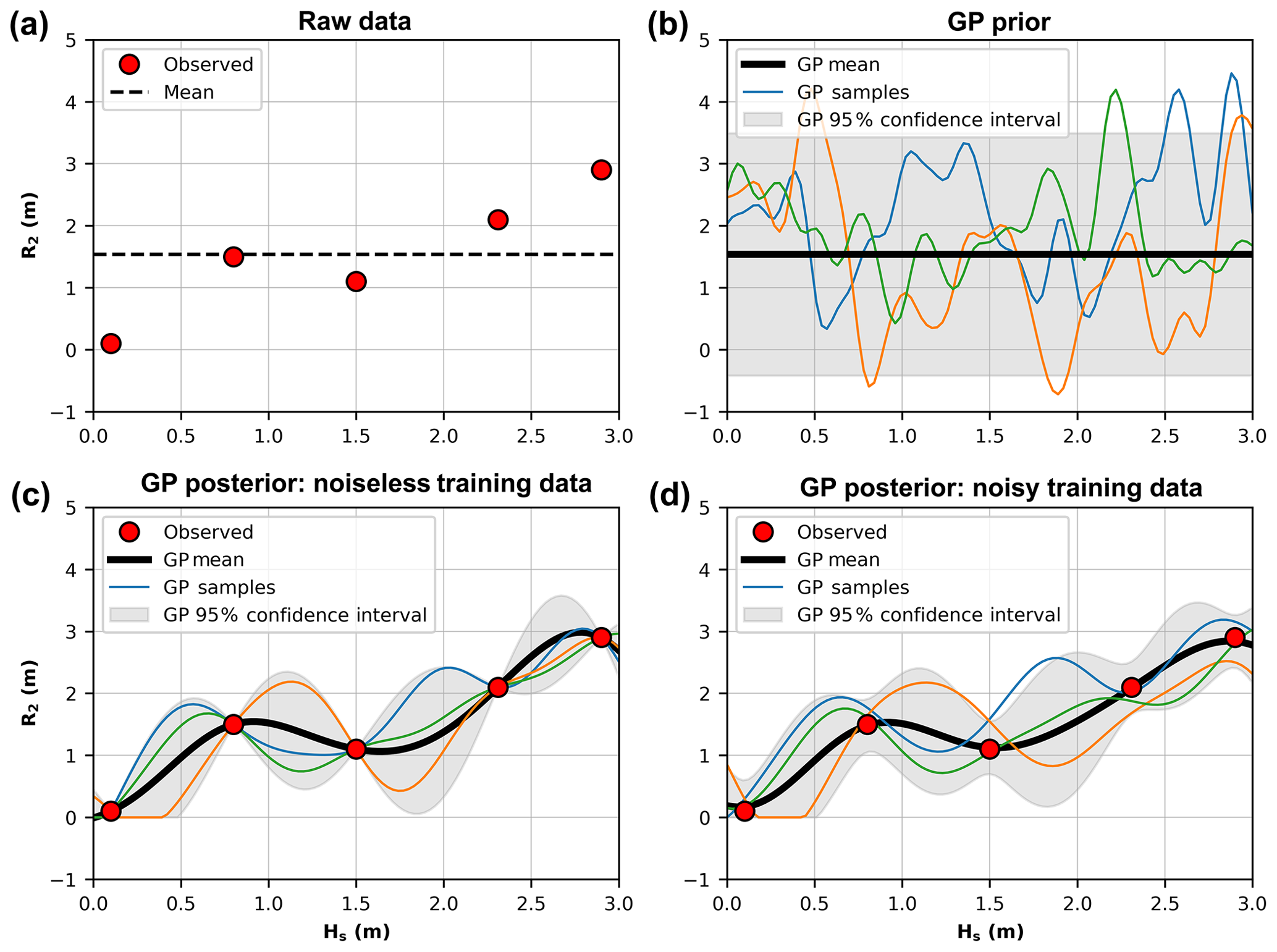
Figure 1(a) Five hypothetical random observations of significant wave height (Hs) and 2 % wave runup elevation (R2). (b) The Gaussian process (GP) prior distribution. (c) The GP posterior distribution, formed by conditioning the prior distribution in (b) with the observed data points in (a), assuming the observations are noise-free. (d) The GP posterior distribution conditioned on the observations with a noise component.
There are many different types of covariance functions or kernels. One of the most common, and the one used in this study, is the squared exponential covariance function:
where σf is the signal variance and l is known as the length scale, both of which are hyperparameters in the model that can be estimated from data (discussed further in Sect. 2.2). Together the mean function and covariance function specify a multivariate Gaussian distribution:
where f is the output of the prior distribution, the mean function is assumed to be 0, and K is the covariance matrix made by evaluating the covariance function at arbitrary input points that lie within the domain being modelled (i.e., K(x, , xj)). Random sample functions can be drawn from this prior distribution as demonstrated in Fig. 1b.
The goal is to determine which of these functions actually fit the observed data points (training data) in Fig. 1a. This can be achieved by forming a posterior distribution on the function space by conditioning the prior with the training data. Roughly speaking, this operation is mathematically equivalent to drawing an infinite number of random functions from the multivariate Gaussian prior (Eq. 3) and then rejecting those that do not agree with the training data. As mentioned above, the multivariate Gaussian offers a simple, closed form solution to this conditioning. Assuming that our observed training data are noiseless (i.e., y exactly represents the value of the underlying function f) then we can condition the prior distribution with the training data samples (x, y) to define a posterior distribution of the function value (f*) at arbitrary test inputs (x*):
where f* is the output of the posterior distribution at the desired test points x*, y is the training data outputs at inputs x, K* is the covariance matrix made by evaluating the covariance function (Eq. 2) between the test inputs x* and training inputs x (i.e., k(x*, x)), K is the covariance matrix made by evaluating the covariance function between training data points x, and is the covariance matrix made by evaluating the covariance function between test points x*. Function values can be sampled from the posterior distribution as shown in Fig. 1c. These samples represent random realizations of what the underlying function describing the training data could look like.
As stated earlier, in Eq. (4) and Fig. 1c there is an assumption that the training data are noiseless and represent the exact value of the function at the specific point in input space. In reality, there is error associated with observations of physical systems, such that
where ε is assumed to be independent identically distributed Gaussian noise with variance . This noise can be incorporated into the GP modelling framework through the use of a white noise kernel that adds an element of Gaussian white noise into the model:
where is the variance of the noise and δij is a Kronecker delta which is 1 if i=j and 0 otherwise. The squared exponential kernel and white noise kernel are closed under addition and product (Rasmussen and Williams, 2006), such that they can simply be combined to form a custom kernel for use in the GP:
The combination of kernels to model different signals in a dataset (that vary over different spatial or temporal timescales) is common in applications of GPs (Rasmussen and Williams, 2006; Reggente et al., 2014; Roberts et al., 2013). Samples drawn from the resultant noisy posterior distribution are shown in Fig. 1d, in which the GP can now be seen to not fit the observed training data precisely.
2.2 Gaussian process kernel optimization
In Eq. (7) there are three hyperparameters: the signal variance (σf), the length scale (l), and the noise variance (σn). These hyperparameters are typically unknown but can be estimated and optimized based on the particular dataset. Here, this optimization is performed by using the typical methodology of maximizing the log marginal likelihood of the observed data y given the hyperparameters:
The Python toolkit scikit-learn (Pedregosa et al., 2011) was used to develop the GP described in this study. For the Reader unfamiliar with the Python programming language, alternative programs for developing Gaussian processes include Matlab (Rasmussen and Nickisch, 2010) and R (Dancik and Dorman, 2008; MacDonald et al., 2015).
2.3 Training a Gaussian process model
It is standard practice in the development of data-driven machine-learning models to divide the available dataset into training, validation, and testing subsets. The training data are used to fit model parameters. The validation data are used to evaluate model performance, and the model hyperparameters are usually varied until performance on the validation data is optimized. Once the model is optimized, the remaining test dataset is used to objectively evaluate its performance and generalizability. A decision must be made about how to split a dataset into training, validation, and testing subsets. There are many different approaches to handle this splitting process; for example, random selection, cross validation, stratified sampling, or a number of other deterministic sampling techniques (Camus et al., 2011). The exact technique used to generate the data subsets often depends on the problem at hand. Here, there were two constraints to be considered: first, the computational expense of GPs scales by O(n3) (Rasmussen and Williams, 2006), so it is desirable to keep the training set as small as possible without deteriorating model performance; and, secondly, machine-learning models typically perform poorly with out-of-sample predictions (i.e., extrapolation), so it is desirable to include in the training set the data samples that capture the full range of variability in the data. Based on these constraints, we used a maximum dissimilarity algorithm (MDA) to divide the available data into training, validation, and testing sets.
The MDA is a deterministic routine that iteratively adds a data point to the training set based on how dissimilar it is to the data already included in the training set. Camus et al. (2011) provide a comprehensive introduction to the MDA selection routine, and it has been previously used in machine-learning studies (e.g., Goldstein et al., 2013). Briefly, to initialize the MDA routine, the data point with the maximum sum of dissimilarity (defined by Euclidean distance) to all other data points is selected as the first data point to be added to the training dataset. Additional data points are included in the training set through an iterative process whereby the next data point added is the one with maximum dissimilarity to those already in the training set – this process continues until a user-defined training set size is reached. In this way the MDA routine produces a set of training data that captures the range of variability present in the full dataset. The data not selected for the training set are equally and randomly split to form the validation dataset and test dataset. While alternative data-splitting routines are available, including simple random sampling, stratified random sampling, self-organizing maps, and k-means clustering (Camus et al., 2011), the MDA routine used in this study was found in preliminary testing (not presented) to produce the best GP performance with the least computational expense.
3.1 Runup data
In 2014, an extended-range lidar (light detection and ranging) device (SICK LD-LRS 2110) was permanently installed on the rooftop of a beachside building (44 m a.m.s.l. – above mean sea level) at Narrabeen–Collaroy Beach (hereafter referred to simply as Narrabeen) on the southeast coast of Australia (Fig. 2). Since 2014, this lidar has continuously scanned a single cross-shore profile transect extending from the base of the beachside building to a range of 130 m, capturing the surface of the beach profile and incident wave swash at a frequency of 5 Hz in both daylight and non-daylight hours. Specific details of the lidar setup and functioning can be found in Phillips et al. (2019).
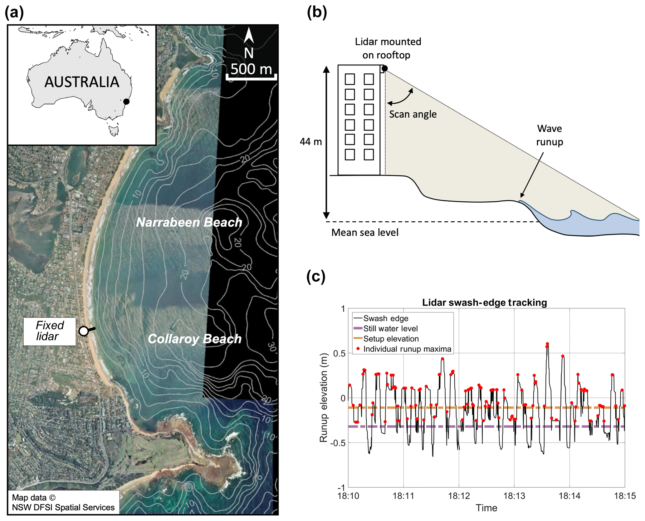
Figure 2(a) Narrabeen Beach, located on the southeast coast of Australia. (b) Conceptual figure of the fixed lidar setup. (c) A 5 min extract of runup elevation extracted from the lidar data; individual runup maxima are marked with red circles.
Narrabeen Beach is a 3.6 km long embayed beach bounded by rocky headlands. It is composed of fine to medium quartz sand (D50≈0.3 mm), with a ∼30 % carbonate fraction. Offshore, the coastline has a steep and narrow (20–70 km) continental shelf (Short and Trenaman, 1992). The region is microtidal and semidiurnal with a mean spring tidal range of 1.6 m and has a moderate to high energy deep water wave climate characterized by persistent long-period south-southeast swell waves that is interrupted by storm events (significant wave height > 3 m) typically 10–20 times per year (Short and Trenaman, 1992). In the present study, approximately 1 year of the high-resolution wave runup lidar dataset available at Narrabeen is used to develop a data-driven parameterization of the 2 % exceedance of wave runup (R2). Data used to develop this parameterization were at hourly resolution and include R2, the beach slope (β), offshore significant wave height (Hs), and peak wave period (Tp). These data are described below and have been commonly used to parameterize R2 in other empirical models of wave runup (e.g., Holman, 1986; Hunt, 1959; Stockdon et al., 2006).
Individual wave runup elevation on the beach profile was extracted on a wave-by-wave basis from the lidar dataset (Fig. 2c) using a neural network runup detection tool developed by Simmons et al. (2019). Hourly R2 was calculated as the 2 % exceedance value for a given hour of wave runup observations. β was calculated as the linear (best-fit) slope of the beach profile over which 2 standard deviations of wave runup values were observed during the hour. Hourly Hs and Tp data were obtained from the Sydney Waverider buoy, situated 11 km offshore of Narrabeen in ∼80 m water depth. Narrabeen is an embayed beach, where prominent rocky headlands both attenuate and refract incident waves. To remove these effects in the wave data and to emulate an open coastline and generalize the parameterization of R2 presented in this study, offshore wave data were first transformed to a nearshore equivalent (10 m water depth) using a precalculated lookup table generated with the SWAN spectral wave model based on a 10 m resolution grid (Booij et al., 1999) and then reverse shoaled back to deep water wave data. A total of 8328 hourly samples of R2, β, Hs, and Tp were extracted to develop a parameterization of R2 in this study. Histograms of these data are shown in Fig. 3.
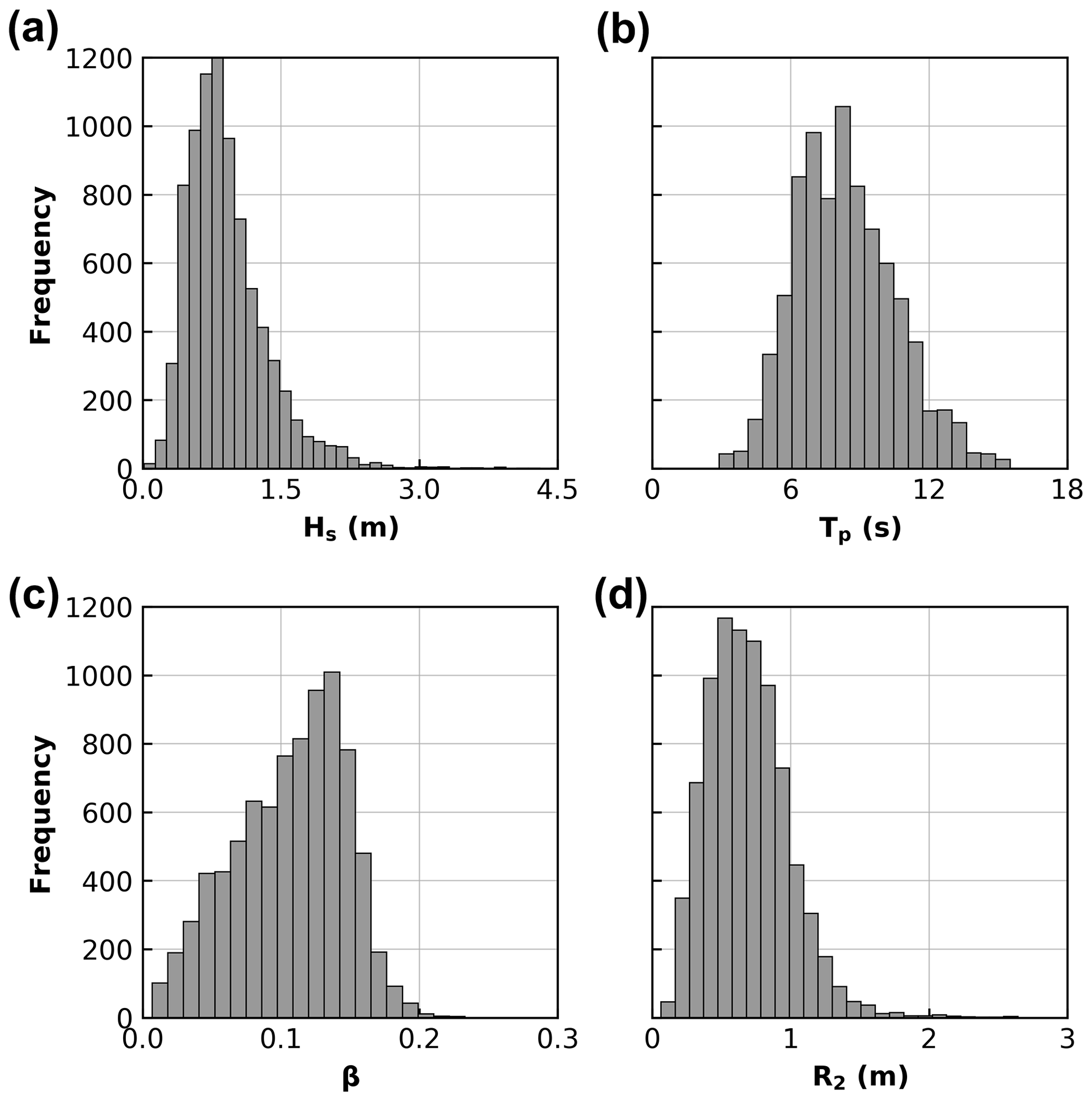
Figure 3Histograms of the 8328 data samples extracted from the Narrabeen lidar: (a) significant wave height (Hs); (b) peak wave period (Tp); (c) beach slope (β); and (d) 2 % wave runup elevation (R2).
3.2 Training data for the GP runup predictor
To determine the optimum training set size, kernel, and model hyperparameters, a number of different user-defined training set sizes were trialled using the MDA selection routine discussed in Sect. 2.3. The GP was trained using different amounts of data and hyperparameters were optimized on the validation dataset only. It was found that a training set size of only 5 % of the available dataset (training dataset: 416 of 8328 available samples; validation dataset: 3956 samples; testing dataset: 3956 samples) was required to develop an optimum GP model. Training data sizes beyond this value produced negligible changes in GP performance but considerable increases in computational demand, similar to findings of previous work (Goldstein and Coco, 2014; Tinoco et al., 2015). Results presented below discuss the performance of the GP on the testing dataset which was not used in GP training or validation.
3.3 Runup predictor results
Results of the GP R2 predictor on the 3956 test samples are shown in Fig. 4. This figure plots the mean GP predictions against corresponding observations of R2. The mean GP prediction performs well on the test data, with a root-mean-squared error (RMSE) of 0.18 m and bias (B) of 0.02 m. For comparison, the commonly used R2 parameterization of Stockdon et al. (2006) tested on the same data has a RMSE of 0.36 m and B of 0.21 m. Despite the relatively accurate performance of the GP on this dataset, there remains significant scatter in the observed versus predicted R2 in Fig. 4. This is consistent with recent work by Atkinson et al. (2017) showing that commonly used predictors of R2 always result in scatter.

Figure 4Observed 2 % wave runup (R2) versus the R2 predicted by the Gaussian process model. The root-mean-squared error (RMSE) is 0.36 m, bias (B) is 0.02 m, and squared correlation (r2) is 0.54.
As discussed in Sect. 1 scatter in runup predictions is likely a result of unresolved processes in the model such as wave dispersion, wave spectrum, nearshore morphology, or a range of other possible processes. Regardless of the origin, here this scatter (uncertainty) is used to form ensemble predictions. The GP developed here not only gives a mean prediction as used in Fig. 4, but it specifies a multivariate Gaussian distribution from which different random functions that describe the data can be sampled. Random samples of wave runup from the GP can capture uncertainty around the mean runup prediction (as was demonstrated in the hypothetical example in Fig. 1d). To assess how well the GP model captures uncertainty, random samples are successively drawn from the GP, and the number of R2 measurements captured with each new draw are determined. Only 10 random samples drawn from the GP are required to capture 95 % of the scatter in R2 (Fig. 5a). This process of drawing random samples from the GP was repeated 100 times with results showing that the above is true for any 10 random samples, with an average capture percentage of 95.7 % and range of 94.9 % to 96.1 % for 10 samples across the 100 trials. As a point of contrast, Fig. 5b shows how much arbitrary error would need to be added to the mean R2 prediction to capture scatter about the mean to emulate the uncertainty captured by the GP. It can be seen that the mean R2 prediction would need to vary by ±51 % to capture 95 % of the scatter present in the runup data. This demonstrates how random models of runup drawn from the GP effectively capture uncertainty in R2 predictions. These randomly drawn R2 models can be used within a larger dune-impact model to produce an ensemble of dune erosion predictions that includes uncertainty in runup predictions, as demonstrated in Sect. 4.
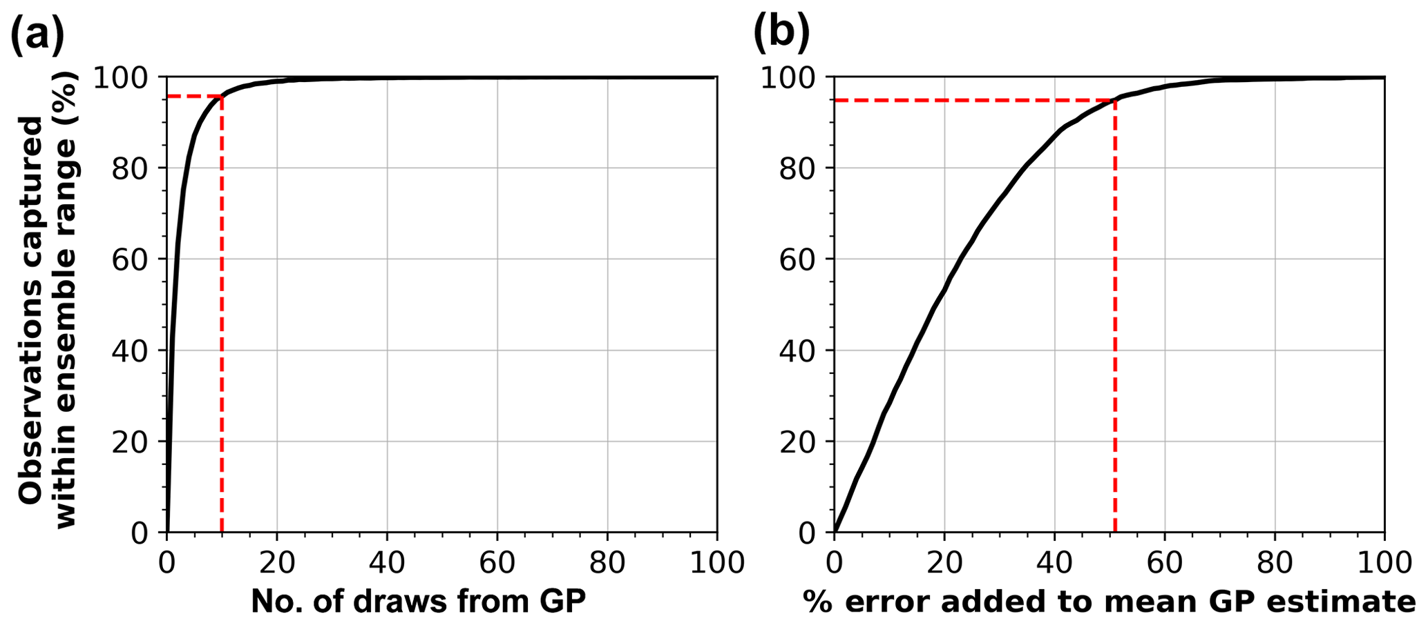
Figure 5(a) Percent of observed runup values captured within the range of ensemble predictions made by randomly sampling different runup values from the Gaussian process. Only 10 randomly drawn models can form an ensemble that captures 95 % of the scatter in observed R2 values. (b) An experiment showing how much arbitrary error would need to be added to the mean GP runup prediction in order to capture scatter in R2 observations. The mean GP prediction would have to vary by 51 % in order to capture 95 % of scatter in R2 observations.
4.1 Dune erosion model
We use the dune erosion model of Larson et al. (2004) as an example of how the GP runup predictor can be used to create an ensemble of dune erosion predictions, and we thus provide probabilistic outcomes with uncertainty bands needed in coastal management. The dune erosion model is subsequently referred to as LEH04 and is defined as follows:
where dV (m3 m−1) is the volumetric dune erosion per unit width alongshore for a given time step t, zb (m) is the time-varying dune toe elevation, T (s) is the wave period for that time step, R2 (m) is the 2 % runup exceedance for that time step, and Cs is the transport coefficient. Note that the original equation used a best-fit relationship to define the runup term, R (see Eq. 36 in Larson et al., 2004), rather than R2. Subsequent modifications of the LEH04 model have been made to adjust the collision frequency (i.e. the t∕T term; e.g., Palmsten and Holman, 2012, and Splinter and Palmsten, 2012); however, we retain the model presented in Eq. (9) for the purpose of providing a simple illustrative example. At each time step, dune volume is eroded in bulk, and the dune toe is adjusted along a predefined slope (defined here as the linear slope between the pre- and post-storm dune toe) so that erosion causes the dune toe to increase in elevation and recede landward. Dune erosion and dune toe recession only occurs when wave runup (R2) exceeds the dune toe (i.e., ) and cannot progress vertically beyond the maximum runup elevation. When R2 does not exceed zb, dV = 0. The GP R2 predictor described in Sect. 3 is used to stochastically parameterize wave runup in the LEH04 model and form ensembles of dune erosion predictions. The model is applied to new data not used to train the GP R2 predictor, using detailed observations of dune erosion caused by a large coastal storm event at Narrabeen Beach, southeast Australia in 2011.
4.2 June 2011 storm data
In June 2011 a large coastal storm event impacted the southeast coast of Australia. This event resulted in variable alongshore dune erosion at Narrabeen Beach, which was precisely captured by airborne lidar immediately pre-, during, and post-storm by five surveys conducted approximately 24 h apart. Cross-shore profiles were extracted from the lidar data at 10 m alongshore intervals as described in detail in Splinter et al. (2018), resulting in 351 individual profiles (Fig. 6). The June 2011 storm lasted 120 h. Hourly wave data were recorded by the Sydney Waverider buoy located in ∼80 m water depth directly to the southeast of Narrabeen Beach. As with the hourly wave data used to develop the GP model of R2 (Sect. 3.1), hourly wave data for each of the 351 profiles for the June 2011 storm were obtained by first transforming offshore wave data to the nearshore equivalent at 10 m water depth directly offshore of each profile using the SWAN spectral wave model (Booij et al., 1999) and then reverse shoaling back to equivalent deep water wave data, to account for the effects of wave refraction and attenuation caused by the distinctly curved Narrabeen embayment. The tidal range during the storm event was measured in situ at the Fort Denison tide gauge (located within Sydney Harbour approximately 16 km south of Narrabeen) as 1.58 m (mean spring tidal range at Narrabeen is 1.6 m). As can be seen in Fig. 6 the wave conditions for the June 2011 storm lie within the range of the training dataset used to develop the GP runup predictor. The hydrodynamic time series and airborne lidar observations of dune change are used to demonstrate how the LEH04 model can be used with the GP predictor of runup to generate stochastic parameterizations and create probabilistic model ensembles (Eq. 9).
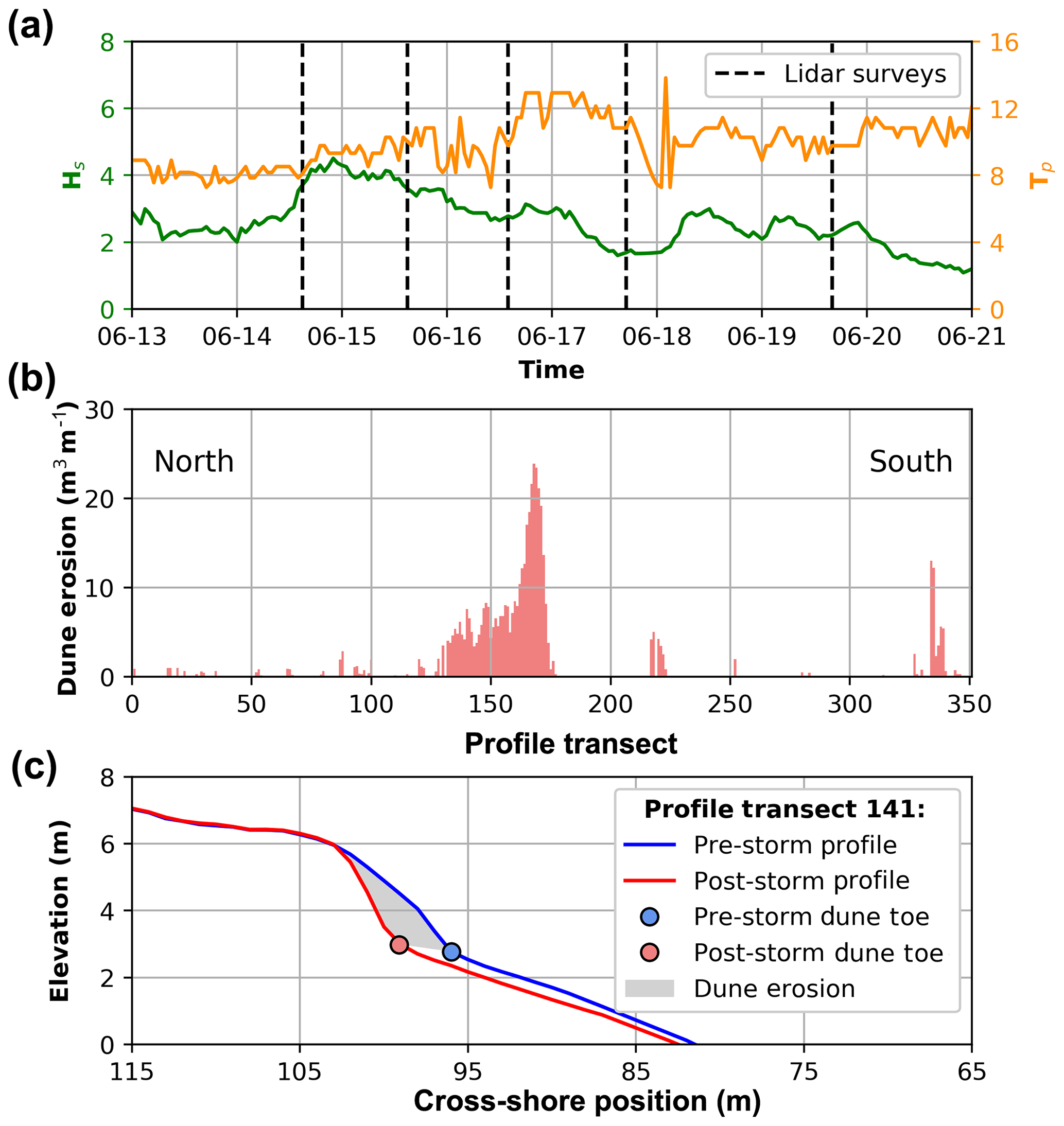
Figure 6June 2011 storm data. (a) Offshore Hs and Tp with vertical dashed lines indicating the time of the lidar surveys, (b) measured (pre- vs. post-storm) dune erosion volumes for the 351 profile transects extracted from lidar data, and (c) example pre- (blue) and post-storm (red) profile cross sections showing dune toes (coloured circles) and dune erosion volume (grey shading).
For each of the 351 available profiles, the pre-, during, and post-storm dune toe positions were defined as the local maxima of curvature of the beach profile following the method of Stockdon et al. (2007). Dune erosion at each profile was then defined as the difference in subaerial beach volume landward of the pre-storm dune toe, as shown in Fig. 6c. Of the 351 profiles, only 117 had storm-driven dune erosion (Fig. 6b). For the example demonstration presented here, only profiles for which the post-storm dune toe elevation was at the same or higher elevation than the pre-storm dune toe are considered, which is a basic assumption of the LEH04 model. Of the 117 profiles with storm erosion, 40 profiles met these criteria. For each of these profiles, the linear slope between the pre- and post-storm dune toe was used to project the dune erosion calculated using the LEH04 model.
The LEH04 dune erosion model (Eq. 9) has a single tuneable parameter, the transport coefficient Cs. There is ambiguity in the literature regarding the value of Cs. Larson et al. (2004) developed an empirical equation to relate Cs to wave height (Hrms) and grain size (D50) using experimental data. Values ranged from to , and Larson et al. (2004) used based on field data from Birkemeier et al. (1988). Palmsten and Holman (2012) used LEH04 to model dune erosion observed in a large wave tank experiment conducted at the O. H. Hinsdale Wave Research Laboratory at Oregon State University. The model was shown to accurately reproduce dune erosion when applied in hourly time steps using a Cs of , based on the empirical equation determined by Larson et al. (2004). Mull and Ruggiero (2014) used values of and as lower and upper bounds of Cs to model dune erosion caused by a large storm event on the Pacific Northwest Coast of the USA and the laboratory experiment used by Palmsten and Holman (2012). For the dune erosion experiment, the value of was found to predict dune erosion volumes closest to the observed erosion when applied in a single time step, with an optimum value of . Splinter and Palmsten (2012) found a best-fit Cs of in an application to modelling dune erosion caused by a large storm event that occurred on the Gold Coast, Australia. Ranasinghe et al. (2012) found a Cs value of in an application at Narrabeen Beach, Australia. It is noted that Cs values in these studies are influenced by the time step used in the model and the exact definition of wave runup, R, used (Larson et al., 2004; Mull and Ruggiero, 2014; Palmsten and Holman, 2012; Splinter and Palmsten, 2012). In practice, Cs could be optimized to fit any particular dataset. However, for predictive applications the optimum Cs value may not be known in advance, since it is unclear if subsequent storms at a given location will be well predicted using previously optimized Cs values. A key goal of this work is to determine if using stochastic parameterizations to generate ensembles that predict a range of dune erosion (based on uncertainty in the runup parameterization) can still capture observed dune erosion even if the optimum Cs value is not known in advance. As such, a Cs value of is used in this example application based on previous work at Narrabeen Beach by Ranasinghe et al. (2012). Sensitivity of model results to the choice of Cs is further discussed in Sect. 4.3.
An example at a single profile (profile 141, located approximately half-way up the Narrabeen embayment as shown in Fig. 6b) of time-varying ensemble dune erosion predictions is provided in Fig. 7. It was previously shown in Fig. 5 that only 10 random samples drawn from the GP R2 predictor were required to capture 95 % of the scatter in the R2 data used to develop and test the GP. However, it is trivial to draw many more samples than this from the GP – for example, drawing 10 000 samples takes less than 1 s on a standard desktop computer. Therefore, to explore a large range of possible runup scenarios during the 120 h storm event, 10 000 different runup time series are drawn from the GP and used to run LEH04 at hourly intervals, thus producing 10 000 model results of dune erosion. The effect of using different ensemble sizes is explored in Sect. 4.3. Figure 7a shows the time-varying distribution of the runup models (blue) used to force LEH04 along with the time-varying prediction distribution of dune toe elevations (grey) throughout the 120 h storm event. To interpret model output probabilistically, the mean of the ensemble is plotted, along with intervals capturing 66 %, 90 %, and 99 % of the ensemble output. These intervals are consistent with those used in IPCC for climate change predictions (Mastrandrea et al., 2010), and, in the context of the model results presented here, they represent varying levels of confidence in the model output. For example, there is high confidence that the real dune erosion will fall within the 66 % ensemble prediction range. Figure 7b shows the time-varying predicted distribution of dune erosion volumes from the 10 000 LEH04 runs. It can be seen that while the mean value of the ensemble predictions deviates slightly from the observed dune erosion, the observed erosion is still captured well within the 66 % envelope of predictions.
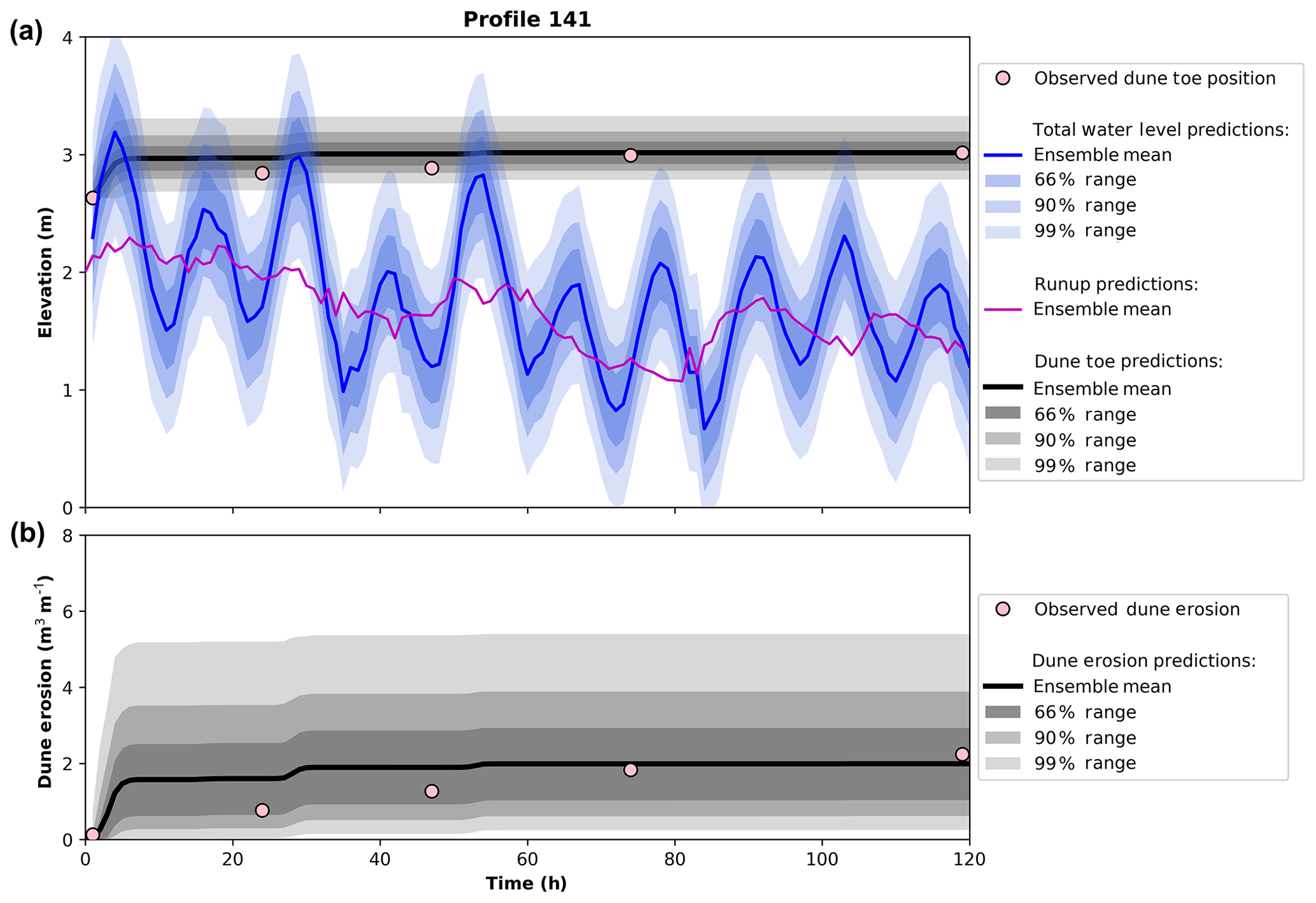
Figure 7Example of LEH04 used with the Gaussian process R2 predictor to form an ensemble of dune erosion predictions. A total of 10 000 runup models are drawn from the Gaussian process and used to force the LEH04 model. (a) Total water level (measured water level + R2; blue) and dune toe elevation (grey) for the 120 h storm event. The bold coloured line is the mean of the ensemble, and shaded areas represent the regions captured by 66 %, 90 %, and 99 % of the ensemble predictions. An example of just the R2 prediction (no measured water level) from the Gaussian process is shown in the magenta line. Pink dots denote the observed dune toe elevation throughout the storm event. (b) The corresponding ensemble of dune erosion predictions.
Pre- and post-storm dune erosion results for the 40 profiles using 10 000 ensemble members and Cs of are shown in Fig. 8. The squared correlation (r2) for the observed and predicted dune erosion volumes is 0.85. Many of the profiles experienced only minor dune erosion (<2.5 m3 m−1) and can be seen to be well predicted by the mean of the ensemble predictions. In contrast, the ensemble mean can be seen to under-predict dune erosion at profiles where high erosion volumes were observed (profiles 29–34 in Fig. 8), with some profiles not even captured by the uncertainty of the ensemble. However, the ensemble range of predictions for these particular profiles also has a large spread, indicative of high uncertainty in predictions and the potential for high erosion to occur. It should be noted that the results presented in Fig. 8 are based on an assumed (i.e., non-optimized) Cs value of . Better prediction of large erosion events could potentially be achieved by increasing Cs or giving greater weighting to these events during calibration, but at the cost of over-predicting the smaller events. The exact effect of varying Cs is quantified in Sect. 4.3. Importantly, Fig. 8 demonstrates that, even with a non-optimized Cs, uncertainty in the GP predictions can provide useful information about the potential for dune erosion, even if the mean dune erosion prediction deviates from the observation – a key advantage of the GP approach over a deterministic approach.

Figure 8Observed (pink dots) and predicted (black dots) dune erosion volumes for the 40 modelled profiles, using 10 000 runup models drawn from the Gaussian process and used to force the LEH04 model. Note that the 40 profiles shown are not uniformly spaced along the 3.5 km Narrabeen embayment. The black dots represent the ensemble mean prediction for each profile, while the shaded areas represent the regions captured by 66 %, 90 %, and 99 % of the ensemble predictions.
4.3 The effect of Cs and ensemble size on dune erosion
In Sect. 4.2, the application of the GP runup predictor within the LEH04 model to produce an ensemble of dune erosion predictions was based on 10 000 ensemble members and a Cs value of . The sensitivity of results to the number of members in the ensemble and the value of the tunable parameter Cs in Eq. (9) is presented in Fig. 9. The mean absolute error (MAE) between the mean ensemble dune erosion predictions and the observed dune erosion, averaged across all 40 profiles, varies for R2 ensembles of 5, 10, 20, 100, 1000, and 10 000 members and Cs values ranging from 10−5 to 10−1 (Fig. 9). As can be seen in Fig. 9a and summarized in Table 1, the lowest MAE for the differing ensemble sizes is similar, ranging from 1.50 to 1.64 m3 m−1, suggesting that the number of ensemble members does not have a significant impact on the resultant mean prediction. The lowest MAE for the different ensemble sizes corresponds to Cs values between (10 000 ensemble members) and (5 ensemble members), which is reasonably consistent with the value of previously reported by Ranasinghe et al. (2012) for Narrabeen Beach and within the range of Cs values presented in Larson et al. (2004).
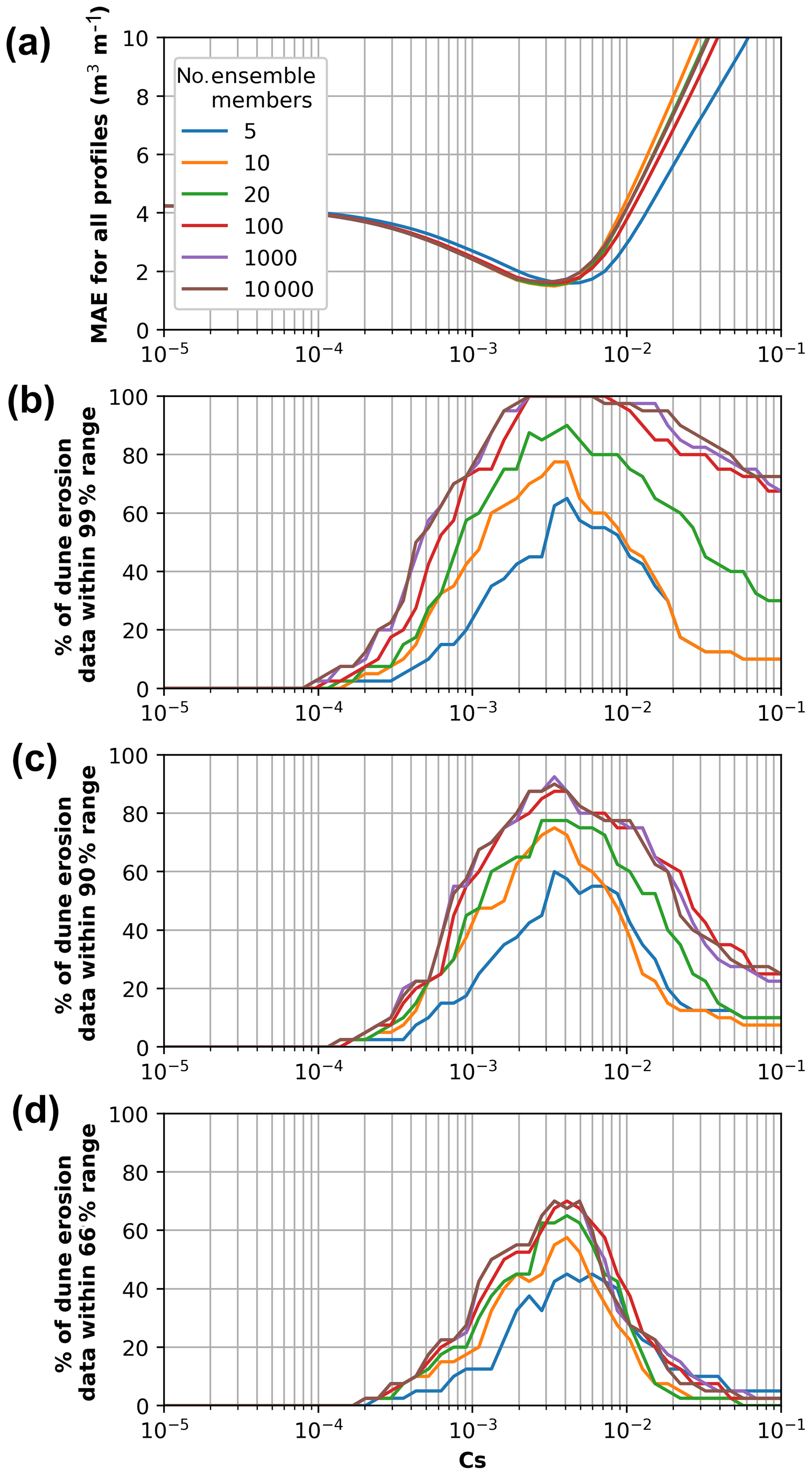
Figure 9Results of the stochastic parameterization methodology for R2 ensembles of 5, 10, 20, 100, 1000, and 10 000 members and Cs values ranging from 10−5 to 10−1. (a) The mean absolute error (MAE) between the median ensemble dune erosion predictions and the observed dune erosion averaged across all 40 profiles. (b–d) show the percentage of dune erosion observations that fall within the 99 %, 90 %, and 66 % ensemble prediction ranges respectively.
The key utility to using a data-driven GP predictor to produce ensembles is that a range of predictions at every location is provided as opposed to a single erosion volume. The ensemble range provides an indication of uncertainty in predictions, which can be highly useful for coastal engineers and managers taking a risk-based approach to coastal hazard management. Figure 9b–d displays the percentage of dune erosion observations from the 40 profiles captured within ensemble predictions for Cs values ranging from 10−5 to 10−1. It can be seen that a high proportion of dune erosion observations are captured within the 66 %, 90 %, and 99 % ensemble envelope across several orders of magnitude Cs. While the main purpose of using ensemble runup predictions within LEH04 is to incorporate uncertainty in the runup prediction, this result demonstrates that the ensemble approach is less sensitive to the choice of Cs than a deterministic model and so can be useful for forecasting with non-optimized model parameters.
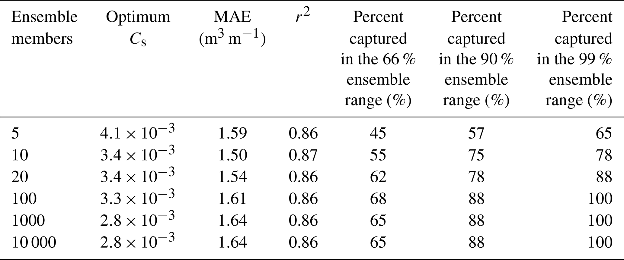
Results in Fig. 9 and Table 1 demonstrate that there is relatively little difference in model performance when more than 10 to 100 ensemble members are used, which is consistent with results presented previously in Fig. 5 that showed that only 10 random samples drawn from the GP R2 predictor were required to capture 95 % of the scatter in the R2 data used to develop and test the GP. This suggests that the GP approach efficiently captures scatter (uncertainty) in runup predictions and subsequently dune erosion predictions, requiring on the order of 10 samples, which is significantly less than the 103–106 runs typically used in Monte Carlo simulations to develop probabilistic predictions (e.g., Callaghan et al., 2008; Li et al., 2013; Ranasinghe et al., 2012).
Table 1Quantitative summary of Fig. 9, showing the optimum Cs value for differing ensemble sizes, along with the associated mean absolute error (MAE) and percent of the 40 dune erosion observations captured by the 66 %, 90 %, and 99 % ensemble prediction range.
5.1 Runup predictors
Studies of commonly used deterministic runup parameterizations such as those proposed by Hunt (1959), Holman (1986), and Stockdon et al. (2006), amongst others, show that these parameterizations are not universally applicable and there remains no perfect predictor of wave runup on beaches (Atkinson et al., 2017; Passarella et al., 2018a; Power et al., 2019). This suggests that the available parameterizations do not fully capture all the relevant processes controlling wave runup on beaches (Power et al., 2019). Recent work has used ensemble and data-driven methods to account for unresolved factors and complexity in runup processes. For example, Atkinson et al. (2017) developed a model of models by fitting a least-squares line to the predictions of several runup parameterizations. Power et al. (2019) used a data-driven, deterministic, gene-expression programming model to predict wave runup against a large dataset of runup observations. Both of these approaches led to improved predictions, when compared to conventional runup parameterizations, of wave runup on the datasets tested in these studies.
The work presented in this study used a data-driven Gaussian process (GP) approach to develop a probabilistic runup predictor. While the mean predictions from the GP predictor developed in this study using high-resolution lidar data of wave runup were accurate (RMSE = 0.18 m) and better than those provided by the Stockdon et al. (2006) formula tested on the same data (RMSE = 0.36 m), the key advantage of the GP approach over deterministic approaches is that probabilistic predictions are output that is specifically derived from data and implicitly accounts for unresolved processes and uncertainty in runup predictions. Previous work has similarly used GPs for efficiently and accurately quantifying uncertainty in other environmental applications (e.g., Holman et al., 2014; Kupilik et al., 2018; Reggente et al., 2014). While alternative approaches are available for generating probabilistic predictions, such as Monte Carlo simulations (e.g., Callaghan et al., 2013), the GP approach offers a method of deriving uncertainty explicitly from data, requires no deterministic equations, and is computationally efficient (i.e., as discussed in Sect. 4.3, drawing 10 000 samples of 120 h runup time series on a standard desktop computer took less than 1 s). However, as discussed in Sect. 2.3, when developing a GP, or any machine-learning model, the training data should include the full range of possible variability in the data to be modelled in order to avoid extrapolation. A limitation of using this data-driven approach for runup prediction is that it can be difficult to acquire a training dataset that captures all possible variability in the system from, for example, longer-term trends in the wave climate, extreme events, or a potentially changing wave climate in the future (Semedo et al., 2012).
5.2 Including uncertainty in dune erosion models
Uncertainty in wave runup predictions within dune-impact models can result in significantly varied predictions of dune erosion. For example, the model of Larson et al. (2004) used in this study only predicts dune erosion if runup elevation exceeds the dune toe elevation and predicts a non-linear relationship between runup that exceeds the dune toe and resultant dune erosion. Hence, if wave runup predictions are biased too low then no dune erosion will be predicted, and if wave runup is predicted too high then dune erosion may be significantly over predicted. Ensemble modelling has become standard practice in many areas of weather and climate modelling (Bauer et al., 2015), as well as hydrological modelling (Cloke and Pappenberger, 2009), and more recently has been applied to coastal problems such as the prediction of cliff retreat (Limber et al., 2018) as a method of handling prediction uncertainty. While using a single deterministic model is computationally simple and provides one solution for a given set of input conditions, model ensembles provide a range of predictions that can better capture the variety of mechanisms and stochasticity within a coastal system. The result is typically improved skill over deterministic models (Atkinson et al., 2017; Limber et al., 2018) and a natural method of providing uncertainty with predictions.
As a quantitative comparison, Splinter et al. (2018) applied a modified version of the LEH04 model to the same June 2011 storm dataset used in the work presented here with a modified expression for the collision frequency (i.e. the t∕T term in Eq. 9) based on work by Palmsten and Holman (2012). The parameterization of Stockdon et al. (2006) was used to estimate R2 in the model. The model was forced hourly over the course of the storm, updating the dune toe, recession slope, and profiles based on each daily lidar survey. Based on only the 40 profiles used in the present study, results from Splinter et al. (2018) showed that the deterministic LEH04 approach reproduced 68 % (r2=0.68) of the observed variability in dune erosion. As shown in Table 1, the simple LEH04 model (Eq. 9) applied here using the GP runup predictor to generate ensemble prediction reproduced ∼85 % (based on the ensemble mean) of the observed variability in dune erosion for the 40 profiles. While there are some discrepancies in the two modelling approaches, the ensemble approach clearly has an appreciable increase in skill over the deterministic approach – attributed here to using a runup predictor trained on local runup data – and the ensemble modelling approach. However, a major advantage of the ensemble approach over the deterministic approach is the provision of prediction uncertainty (e.g., Fig. 8). While the mean ensemble prediction is not 100 % accurate, Table 1 shows that using just 100 samples can capture all the observed variability in dune erosion within the ensemble output.
The GP approach is a novel approach to building model ensembles to capture uncertainty. Previous work modelling beach and dune erosion has successfully used Monte Carlo methods, which randomly vary model inputs within many thousands of model iterations, to produce ensembles and probabilistic erosion predictions (e.g., Callaghan et al., 2008; Li et al., 2013; Ranasinghe et al., 2012). As discussed earlier in Sect. 4.3, the GP approach differs from Monte Carlo in that it explicitly quantifies uncertainty directly from data, does not use deterministic equations, and can be computationally efficient.
For coastal managers, the accurate prediction of wave runup as well as dune erosion is critical for characterizing the vulnerability of coastlines to wave-induced flooding, erosion of dune systems, and wave impacts on adjacent coastal infrastructure. While many formulations for wave runup have been proposed over the years, none have proven to accurately predict runup over a wide range of conditions and sites of interest. In this contribution, a Gaussian process (GP) with over 8000 high-resolution lidar-derived wave runup observations was used to develop a probabilistic parameterization of wave runup that quantifies uncertainty in runup predictions. The mean GP prediction performed well on unseen data, with a RMSE of 0.18 m, which is a significant improvement over the commonly used R2 parameterization of Stockdon et al. (2006) (RMSE of 0.36 m) used on the same data. Further, only 10 randomly drawn models from the probabilistic GP distribution were needed to form an ensemble that captured 95 % of the scatter in the test data.
Coastal dune-impact models offer a method of predicting dune erosion deterministically. As an example application of how the GP runup predictor can be used in geomorphic systems, the uncertainty in the runup parameterization was propagated through a deterministic dune erosion model to generate ensemble model predictions and provide prediction uncertainty. The hybrid dune erosion model performed well on the test data, with a squared correlation (r2) between the observed and predicted dune erosion volumes of 0.85. Importantly, the probabilistic output provided uncertainty bands of the expected erosion volumes, which is a key advantage over deterministic approaches. Compared to traditional methods of producing probabilistic predictions such as Monte Carlo, the GP approach has the advantage of learning uncertainty directly from observed data, it requires no deterministic equations, and is computationally efficient.
This work is an example of how a machine-learning model such as a GP can profitably be integrated into coastal morphodynamic models (Goldstein and Coco, 2015) to provide probabilistic predictions for nonlinear, multidimensional processes, and drive ensemble forecasts. Approaches combining machine-learning methods with traditional coastal science and management models present a promising area for furthering coastal morphodynamic research. Future work is focused on using more data and additional inputs, such as offshore bar morphology and wave spectra, to improve the GP runup predictor developed here, testing it at different locations and integrating it into a real-time coastal erosion forecasting system.
The data and code used to develop the Gaussian process runup predictor in this paper are publicly available at https://doi.org/10.5281/zenodo.3401739 (Beuzen and Goldstein, 2019).
The order of the authors' names reflects the size of their contribution to the writing of this paper.
The authors declare that they have no conflict of interest.
This article is part of the special issue “Advances in computational modelling of natural hazards and geohazards”.
Wave and tide data were kindly provided by the Manly Hydraulics Laboratory under the NSW Coastal Data Network Program managed by OEH. The lead author is funded under the Australian Postgraduate Research Training Program.
This research has been supported by the Australian Research Council (grant nos. LP04555157, LP100200348, and DP150101339), the NSW Environmental Trust Environmental Research Program (grant no. RD 2015/0128), and the DOD DARPA (grant no. R0011836623/HR001118200064).
This paper was edited by Randall LeVeque and reviewed by two anonymous referees.
Atkinson, A. L., Power, H. E., Moura, T., Hammond, T., Callaghan, D. P., and Baldock, T. E.: Assessment of runup predictions by empirical models on non-truncated beaches on the south-east Australian coast, Coast. Eng., 119, 15–31, 2017.
Bauer, P., Thorpe, A., and Brunet, G.: The quiet revolution of numerical weather prediction, Nature, 525, 47–55, 2015.
Berner, J., Achatz, U., Batté, L., Bengtsson, L., Cámara, A. D. L., Christensen, H. M., Colangeli, M., Coleman, D. R., Crommelin, D., Dolaptchiev, S. I., and Franzke, C. L.: Stochastic parameterization: Toward a new view of weather and climate models, B. Am. Meteorol. Soc., 98, 565–588, 2017.
Beuzen, T. and Goldstein, E. B.: TomasBeuzen/BeuzenEtAl_2019_NHESS_GP_runup_model: First release of repo (Version 0.1), Zenodo, https://doi.org/10.5281/zenodo.3401739, 2019.
Beuzen, T., Splinter, K. D., Turner, I. L., Harley, M. D., and Marshall, L.: Predicting storm erosion on sandy coastlines using a Bayesian network, in: Proceedings of Australasian Coasts & Ports: Working with Nature, 21–23 June 2017, Cairns, Australia, 102–108, 2017.
Beuzen, T., Splinter, K., Marshall, L., Turner, I., Harley, M., and Palmsten, M.: Bayesian Networks in coastal engineering: Distinguishing descriptive and predictive applications, Coast. Eng., 135, 16–30, 2018.
Birkemeier, W. A., Savage, R. J., and Leffler, M. W.: A collection of storm erosion field data, Coastal Engineering Research Center, Vicksburg, MS, 1988.
Booij, N., Ris, R. C., and Holthuijsen, L. H.: A third-generation wave model for coastal regions: 1. Model description and validation, J. Geophys. Res.-Oceans, 104, 7649–7666, https://doi.org/10.1029/98jc02622, 1999.
Buchanan, M.: Ignorance as strength, Nat. Phys., 14, 428, https://doi.org/10.1038/s41567-018-0133-9, 2018.
Callaghan, D. P., Nielsen, P., Short, A., and Ranasinghe, R.: Statistical simulation of wave climate and extreme beach erosion, Coast. Eng., 55, 375–390, https://doi.org/10.1016/j.coastaleng.2007.12.003, 2008.
Callaghan, D. P., Ranasinghe, R., and Roelvink, D.: Probabilistic estimation of storm erosion using analytical, semi-empirical, and process based storm erosion models, Coast. Eng., 82, 64–75, 2013.
Camus, P., Mendez, F. J., Medina, R., and Cofiño, A. S.: Analysis of clustering and selection algorithms for the study of multivariate wave climate, Coast. Eng., 58, 453–462, 2011.
Cloke, H. and Pappenberger, F.: Ensemble flood forecasting: A review, J. Hydrol., 375, 613–626, 2009.
Cohn, N. and Ruggiero, P.: The influence of seasonal to interannual nearshore profile variability on extreme water levels: Modeling wave runup on dissipative beaches, Coast. Eng., 115, 79–92, 2006.
Dancik, G. M. and Dorman, K. S.: mlegp: statistical analysis for computer models of biological systems using R, Bioinformatics, 24, 1966–1967, 2008.
den Heijer, C., Knipping, D. T. J. A., Plant, N. G., van Thiel de Vries, J. S. M., Baart, F., and van Gelder, P. H. A. J. M.: Impact Assessment of Extreme Storm Events Using a Bayesian Network, Paper presented at the Coastal Engineering (No. 33), Santander, Spain, 2012.
Erikson, L. H., Larson, M., and Hanson, H.: Laboratory investigation of beach scarp and dune recession due to notching and subsequent failure, Mar. Geol., 245, 1–19, 2007.
García-Medina, G., Özkan-Haller, H. T., Holman, R. A., and Ruggiero, P.: Large runup controls on a gently sloping dissipative beach, J. Geophys. Res.-Oceans, 122, 5998–6010, 2017.
Goldstein, E. B. and Coco, G.: A machine learning approach for the prediction of settling velocity, Water Resour. Res., 50, 3595–3601, 2014.
Goldstein, E. B. and Coco, G.: Machine learning components in deterministic models: hybrid synergy in the age of data, Front. Environ. Sci., 33, 1–4, 2015.
Goldstein, E. B. and Moore, L. J.: Stability and bistability in a one-dimensional model of coastal foredune height, J. Geophys. Res.-Earth Surf., 121, 964–977, 2016.
Goldstein, E. B., Coco, G., and Murray, A. B.: Prediction of wave ripple characteristics using genetic programming, Cont. Shelf Res., 71, 1–15, 2013.
Goldstein, E. B., Coco, G., and Plant, N. G.: A Review of Machine Learning Applications to Coastal Sediment Transport and Morphodynamics, Earth Sci. Rev., 194, 97–108, https://doi.org/10.1016/j.earscirev.2019.04.022, 2019.
Guedes, R., Bryan, K. R., and Coco, G.: Observations of wave energy fluxes and swash motions on a low-sloping, dissipative beach, J. Geophys. Res.-Oceans, 118, 3651–3669, 2013.
Guza, R. and Feddersen, F.: Effect of wave frequency and directional spread on shoreline runup, Geophys. Res. Lett., 39, 1–5, https://doi.org/10.1029/2012GL051959, 2012.
Holman, D., Sridharan, M., Gowda, P., Porter, D., Marek, T., Howell, T., and Moorhead, J.: Gaussian process models for reference ET estimation from alternative meteorological data sources, J. Hydrol., 517, 28–35, 2014.
Holman, R.: Extreme value statistics for wave run-up on a natural beach, Coast. Eng., 9, 527–544, 1986.
Hunt, I. A.: Design of sea-walls and breakwaters, T. Am. Soc. Civ. Eng., 126, 542–570, 1959.
Krasnopolsky, V. M. and Fox-Rabinovitz, M. S.: Complex hybrid models combining deterministic and machine learning components for numerical climate modeling and weather prediction, Neural Networks, 19, 122–134, 2006.
Kupilik, M., Witmer, F. D., MacLeod, E.-A., Wang, C., and Ravens, T.: Gaussian Process Regression for Arctic Coastal Erosion Forecasting, IEEE T. Geosci. Remote, 99, 1–9, 2018.
Larson, M., Erikson, L., and Hanson, H.: An analytical model to predict dune erosion due to wave impact, Coast. Eng., 51, 675–696, 2004.
Li, F., Van Gelder, P., Callaghan, D., Jongejan, R., Heijer, C. D., and Ranasinghe, R.: Probabilistic modeling of wave climate and predicting dune erosion, J. Coast. Res., 65, 760–765, 2013.
Limber, P. W., Barnard, P. L., Vitousek, S., and Erikson, L. H.: A model ensemble for projecting multidecadal coastal cliff retreat during the 21st century, J. Geophys. Res.-Ea. Surf., 123, 1566–1589, 2018.
MacDonald, B., Ranjan, P., and Chipman, H.: GPfit: An R package for fitting a Gaussian process model to deterministic simulator outputs, J. Stat. Softw., 64, 1–23, 2015.
Mastrandrea, M. D., Field, C. B., Stocker, T. F., Edenhofer, O., Ebi, K. L., Frame, D. J., Held, H., Kriegler, E., Mach, K. J., Matschoss, P. R., and Plattner, G. K.: Guidance note for lead authors of the IPCC fifth assessment report on consistent treatment of uncertainties, Intergovernmental Panel on Climate Change (IPCC), 2010.
Mull, J. and Ruggiero, P.: Estimating storm-induced dune erosion and overtopping along US West Coast beaches, J. Coast. Res., 30, 1173–1187, 2014.
Overbeck, J. R., Long, J. W., and Stockdon, H. F.: Testing model parameters for wave-induced dune erosion using observations from Hurricane Sandy, Geophys. Res. Lett., 44, 937–945, 2017.
Palmsten, M. L. and Holman, R. A.: Laboratory investigation of dune erosion using stereo video, Coast. Eng., 60, 123–135, 2012.
Palmsten, M. L., Splinter, K. D., Plant, N. G., and Stockdon, H. F.: Probabilistic estimation of dune retreat on the Gold Coast, Australia, Shore Beach, 82, 35–43, 2014.
Parker, K., Ruggiero, P., Serafin, K. A., and Hill, D. F.: Emulation as an approach for rapid estuarine modeling, Coast. Eng., 150, 79–93, 2019.
Passarella, M., De Muro, S., Ruju, A., and Coco, G.: An assessment of swash excursion predictors using field observations, J. Coast. Res., 85, 1036–1040, 2018a.
Passarella, M., Goldstein, E. B., De Muro, S., and Coco, G.: The use of genetic programming to develop a predictor of swash excursion on sandy beaches, Nat. Hazards Earth Syst. Sci., 18, 599–611, https://doi.org/10.5194/nhess-18-599-2018, 2018b.
Pedregosa, F., Varoquaux, G., Gramfort, A., Michel, V., Thirion, B., Grisel, O., Blondel, M., Prettenhofer, P., Weiss, R., Dubourg, V., and Vanderplas, J.: Scikit-learn: Machine learning in Python, J. Mach. Learn. Res., 12, 2825–2830, 2011.
Phillips, M. S., Blenkinsopp, C. E., Splinter, K. D., Harley, M. D., and Turner, I. L.: Modes of berm and beachface recovery following storm reset: observations using a continuously scanning lidar, J. Geophys. Res.-Ea. Surf., 124, 720–736, 2019.
Plant, N. G. and Stockdon, H. F.: Probabilistic prediction of barrier-island response to hurricanes, J. Geophys. Res.-Ea. Sur., 117, F03015, https://doi.org/10.1029/2011jf002326, 2012.
Power, H. E., Gharabaghi, B., Bonakdari, H., Robertson, B., Atkinson, A. L., and Baldock, T. E.: Prediction of wave runup on beaches using Gene-Expression Programming and empirical relationships, Coast. Eng., 144, 47–61, 2019.
Ranasinghe, R., Callaghan, D., and Stive, M. J.: Estimating coastal recession due to sea level rise: beyond the Bruun rule, Climatic Change, 110, 561–574, 2012.
Rasmussen, C. E. and Nickisch, H.: Gaussian processes for machine learning (GPML) toolbox, J. Mach. Learn. Res., 11, 3011–3015, 2010.
Rasmussen, C. E. and Williams, C. K.: Gaussian Processes for Machine Learning, The MIT Press, Cambridge, Massachusetts, 2006.
Reggente, M., Peters, J., Theunis, J., Van Poppel, M., Rademaker, M., Kumar, P., and De Baets, B.: Prediction of ultrafine particle number concentrations in urban environments by means of Gaussian process regression based on measurements of oxides of nitrogen, Environ. Model. Softw., 61, 135–150, 2014.
Roberts, S., Osborne, M., Ebden, M., Reece, S., Gibson, N., and Aigrain, S.: Gaussian processes for time-series modelling, Philos. T. Roy. Soc. A, 371, 20110550, https://doi.org/10.1098/rsta.2011.0550, 2013.
Roelvink, D., Reniers, A., van Dongeren, A., van Thiel de Vries, J., McCall, R., and Lescinski, J.: Modelling storm impacts on beaches, dunes and barrier islands, Coast. Eng., 56, 1133–1152, https://doi.org/10.1016/j.coastaleng.2009.08.006, 2009.
Ruggiero, P., Komar, P. D., McDougal, W. G., Marra, J. J., and Beach, R. A.: Wave runup, extreme water levels and the erosion of properties backing beaches, J. Coast. Res., 17, 407–419, 2001.
Sallenger, A. H.: Storm impact scale for barrier islands, J. Coast. Res., 16, 890–895, 2000.
Semedo, A., Weisse, R., Behrens, A., Sterl, A., Bengtsson, L., and Günther, H.: Projection of global wave climate change toward the end of the twenty-first century, J. Climate, 26, 8269–8288, 2012.
Short, A. D. and Trenaman, N.: Wave climate of the Sydney region, an energetic and highly variable ocean wave regime, Mar. Freshwater Res., 43, 765–791, 1992.
Simmons, J. A., Splinter, K. D., Phillips, M. S., and Leaman, C. K.: Wave runup detection from Lidar using machine learning techniques, Environ. Model. Softw., in preparation, 2019.
Splinter, K. D. and Palmsten, M. L.: Modeling dune response to an East Coast Low, Mar. Geol., 329, 46–57, 2012.
Splinter, K. D., Kearney, E. T., and Turner, I. L.: Drivers of alongshore variable dune erosion during a storm event: Observations and modelling, Coast. Eng., 131, 31–41, 2018.
Stockdon, H. F., Holman, R. A., Howd, P. A., and Sallenger, A. H.: Empirical parameterization of setup, swash, and runup, Coast. Eng., 53, 573–588, https://doi.org/10.1016/j.coastaleng.2005.12.005, 2006.
Stockdon, H. F., Sallenger Jr., A. H., Holman, R. A., and Howd, P. A.: A simple model for the spatially-variable coastal response to hurricanes, Mar. Geol., 238, 1–20, 2007.
Tinoco, R., Goldstein, E., and Coco, G.: A data-driven approach to develop physically sound predictors: Application to depth-averaged velocities on flows through submerged arrays of rigid cylinders, Water Resour. Res., 51, 1247–1263, 2015.
Van Oorschot, J. and d'Angremond, K.: The effect of wave energy spectra on wave run-up, Coast. Eng., 1968, 888–900, 1969.
- Abstract
- Introduction
- Gaussian processes
- Development of a Gaussian process runup model
- Application of a Gaussian process runup predictor in a coastal dune erosion model
- Discussion
- Conclusion
- Code and data availability
- Author contributions
- Competing interests
- Special issue statement
- Acknowledgements
- Financial support
- Review statement
- References