A physics-based probabilistic forecasting model for rainfall-induced shallow landslides at regional scale

Conventional outputs of physics-based landslide forecasting models are presented as deterministic warnings by calculating the safety factor (F_s) of potentially dangerous slopes. However, these models are highly dependent on variables such as cohesion force and internal friction angle which are affected by a high degree of uncertainty especially at a regional scale, resulting in unacceptable uncertainties of F_s. Under such circumstances, the outputs of physical models are more suitable if presented in the form of landslide probability values. In order to develop such models, a method to link the uncertainty of soil parameter values with landslide probability is devised. This paper proposes the use of Monte Carlo methods to quantitatively express uncertainty by assigning random values to physical variables inside a defined interval. The inequality F_s<1 is tested for each pixel in n simulations which are integrated in a unique parameter. This parameter links the landslide probability to the uncertainties of soil mechanical parameters and is used to create a physics-based probabilistic forecasting model for rainfall-induced shallow landslides. The prediction ability of this model was tested in a case study, in which simulated forecasting of landslide disasters associated with heavy rainfalls on 9 July 2013 in the Wenchuan earthquake region of Sichuan province, China, was performed. The proposed model successfully forecasted landslides in 159 of the 176 disaster points registered by the geo-environmental monitoring station of Sichuan province. Such testing results indicate that the new model can be operated in a highly efficient way and show more reliable results, attributable to its high prediction accuracy. Accordingly, the new model can be potentially packaged into a forecasting system for shallow landslides providing technological support for the mitigation of these disasters at regional scale.

1 Introduction

Rainfall-induced shallow landslides are common in many mountainous areas and are considered extremely dangerous (Varnes, 1978). Despite the low volume of debris deposits involved in these processes (generally <1000 m³), rainfall-induced shallow landslides present high moving speeds (Cruden and Varnes, 1996), evolve very rapidly, and can propagate even in presence of obstacles (Davide and Davide, 2010). Current regional landslide forecasting models mainly focuses on shallow landslides. They can be classified in three categories: statistics-based methods (Caine, 1980; Crosta, 1998; Crosta and Frattini, 2001; Aleotti, 2004; Wei et al., 2004; Wieczorek and Glade, 2005; Cardinali et al., 2006; Jacob et al., 2006), contributor-factor-based forecasting methods (Dai and Lee, 2003; Wei et al., 2007a; Chang et al., 2008) and physics-based forecasting methods (Montgomery and Dietrich, 1994; Wu and Sidle, 1995; Montgomery et al., 1998; Iverson, 2000; Wilkinson et al., 2002; Crosta and Frattini, 2003; Salciarini et al., 2006). The physics-based forecasting models have overcome the drawback of statistics-based models with respect to excessive dependence on rainfall data. Furthermore, by devising mechanisms for coupling rainfall with soil surface mechanics using hydrological process simulation (Zhang et al., 2014a), the physically based models represent an improvement over the independent treatment of these factors by contributor-factor-based forecasting models (e.g., Wei et al., 2007a).

The physics-based forecasting model is able to describe the variation rule of hydrological parameters induced by rainfall infiltration and further explain the failure mechanism of a slope due to the variation of hydrological parameters. Those characteristics explain the interest of scholars in the physics-based forecasting model and its implementation at regional scales (Schmidt et al., 2008; Montrasio et al., 2011; Raia et al., 2014). The most common analysis unit used in physics-based forecasting models is the pixel, used for example in the well-known TRIGRS model (Transient Rainfall Infiltration and Grid-Based Regional Slope-Stability Analysis; Baum, et al., 2002, 2008). The safety factor of each pixel within a forecasting region F_s ($F_{\mathrm{s}}=R/S$, where R is shear resistance and S is the driving force) is calculated considering rainfall infiltration; pixels are then identified as unstable (F_s<1) or stable (F_s≥1). From these results, landslide warnings are expressed deterministically by labeling each pixel of the forecasting area as either “landslide occurrence” or “nonoccurrence”.

However, it must be noted that the underlying physics-based forecasting model requires a large number of surface data to be assigned to each pixel before safety factors can be calculated. The physics-based model is sensitive to the accuracy of such data, especially the soil mechanical parameters (cohesion force and internal friction angle) that can significantly influence the pixel stability. In general, and specially for large areas, seemingly deterministic soil mechanical parameters at pixel level used in physical models have different amounts of uncertainty (Schmidt et al., 2008; Rossi et al., 2013), which thus generate uncertain forecasting results. In this scenario, it is unwise to give deterministic forecasting results to the public while using the physical model in local forecasting service.

Providing probabilistic landslide forecasting results is the more direct solution to this issue. Currently, several scholars are advancing in the development of physics-based probabilistic forecasting models (Schmidt et al., 2008; Raia et al., 2014). However, the relationship between the landslide probability and the uncertainties in soil mechanical parameters is not addressed in their models. This effectively renders such probabilistic models actually still in the deterministic mode. For example, a series of deterministic forecasting results are generated by the model during the simulation process (Raia et al., 2014); an experienced forecaster with professional knowledge of landslides is necessary in order to identify the most probable one. Consequently, this approach requires a large number of calculations, which is unsuitable for operational forecasting of shallow landslides.

This paper focuses on an effective method for linking landslide probability to the uncertain soil mechanical parameters. It uses Monte Carlo methods to propose a probabilistic forecasting model with a high calculating efficiency. The proposed model can directly generate probabilistic forecasting results instead of serial deterministic results, and hence it will be more suitable to operational forecasting of shallow landslides, especially at the regional scale.

The next section introduces the physics-based probabilistic forecasting for a shallow-landslide model. The third section addresses the general aspects of its application to a regional-scale shallow-landslide forecasting system. The fourth section describes a case study in which the effectiveness of the proposed model is analyzed in a study case. Sections 5 and 6 discuss the results and state the conclusions of this study, respectively.

2 Probabilistic forecasting for shallow landslides

2.1 The infinite-slope model for unsaturated soil slopes using safety factor F_s

There are two mechanisms that trigger failure in slopes subject to rainfall infiltration. They are loss of matrix suction and increasing of a positive pore water pressure (Li et al., 2013). In southwestern China, precipitation is rich in summer due to monsoon conditions from both the Pacific and India Ocean (Wei et al., 2006). Before the rainy season, slopes in this area are generally unsaturated during the relatively dry seasons. Almost all landslide disasters in southwestern China occur during the rainy season when the matrix suction of topsoil suddenly decreases due to heavy monsoon rains. Consequently, this research focuses on the stability analysis of unsaturated soil mass.

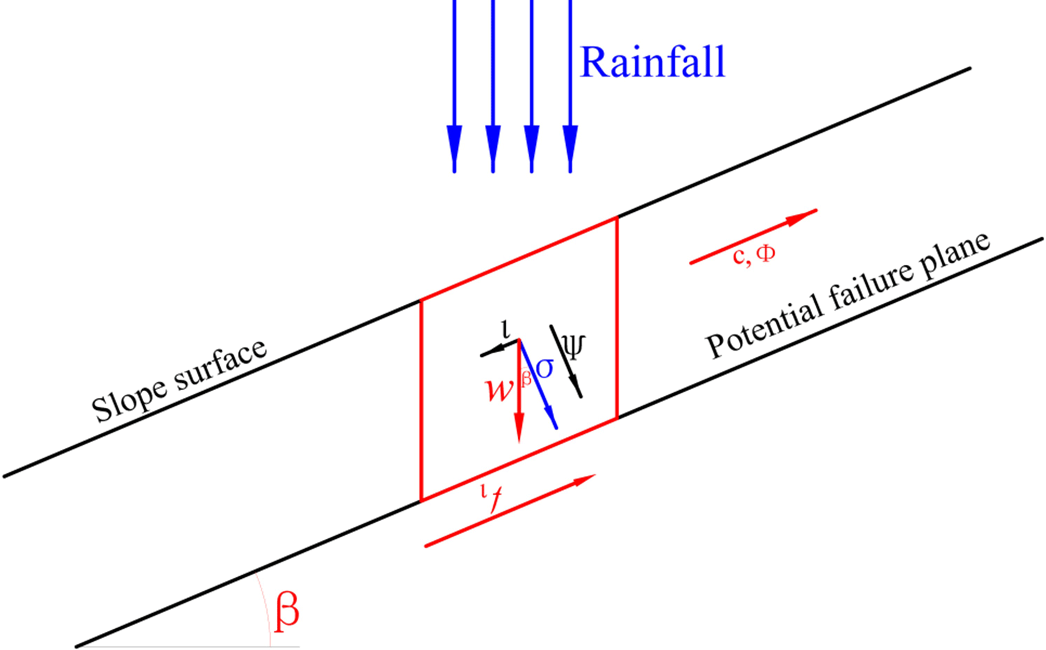
During the evolution process from stability to failure driven by rainfall infiltration, the rapid loss of suction due to the increasing soil water content is the key triggering factor for shallow landslides. The safety factor F_s is used to evaluate the stability of slopes under the action of rainfall infiltration; in this scenario, the failure plane is governed by the Mohr–Coulomb failure criteria of unsaturated soil mass and is assumed to be parallel to the slope surface (Fig. 1). The expression of F_s based on the shear strength formula of the unsaturated soil (Fredlund and Rahardjo, 1993) and the infinite-slope model can be expressed as follows:

$$\begin{array}{}\text{(1)}& F_{\mathrm{s}}={\displaystyle \frac{\tan \mathit{\phi }}{\tan \mathit{\beta }}}+{\displaystyle \frac{c+\mathit{\psi }\tan \left({\mathit{\phi }}^{\mathrm{b}}\right)}{{\mathit{\gamma }}_t{H}_{\mathrm{s}}\cos \mathit{\beta }\sin \mathit{\beta }}},\end{array}$$

where c is stress and can be named the cohesion force; φ is the internal friction angle; φ^b is related to the matrix suction (which is close to the internal friction angle φ in the condition of the low matrix suction); H_s is the instable soil depth; and ψ is the matrix suction of the soil, which is a function of the soil water content described as follows (Van Genuchten, 1980):

$$\begin{array}{}\text{(2)}& S_{\mathrm{e}}={\displaystyle \frac{\mathit{\theta }-{\mathit{\theta }}_{\mathrm{r}}}{{\mathit{\theta }}_{\mathrm{s}}-{\mathit{\theta }}_{\mathrm{r}}}}={\left[{\displaystyle \frac{\mathrm{1}}{\mathrm{1}+(\mathit{\alpha }\times \mathit{\psi }{)}^n}}\right]}^m,\end{array}$$

where S_e is the saturation degree; θ_s is the saturated water content; θ_r is the residual water content; θ is the soil water content of the current hour; α, n and m are the parameters of soil water characteristic curve; and $n=\mathrm{1}-\mathrm{1}/m$.

Figure 1 Infinite-slope model for unsaturated soil on a slope.

2.2 Deterministic forecasting model using safety factor F_s

The infinite-slope model aims to calculate the safety factor F_s to identify the stability of a slope. It has its basis in a theoretical hypothesis (Apip et al., 2010), which can describe the mechanical process of shallow-landslide formation. This approach can give reliable results for each pixel as long as the soil mechanical parameters are accurate. From a deterministic point of view, this physical framework can be briefly drawn as follows: for each pixel in the forecast area, if F_s<1, it is considered unstable, while pixels with F_s≥1 are considered to be stable.

Acquiring the values for the soil mechanical parameters necessary for the infinite-slope model require the use of field sampling or soil-texture-based methods (Blondeau, 1973; Apip et al., 2010; Zhang et al., 2014a, b). However, the precision of these methods is relatively low (Schmidt et al., 2008), and they are thus subject to high levels of uncertainty. Consequently, the seemingly deterministic infinite-slope model based on soil mechanical parameters of each pixel is in fact uncertain (Schmidt et al., 2008; Rossi et al., 2013). This will be reflected in the safety factors F_s of each pixel, leading to a situation in which, despite the advantages of the physically based landslide forecasting model, it may be misleading if used in a deterministic way for real-world applications.

This is not an issue for other landslide forecasting models. For example, although the input variables of the contribution-factor-based forecasting model are also uncertain (Wei et al., 2007a), and thus it is essentially a statistical model (Zhang et al., 2014a), it successfully accounts for the relationship between uncertainties of input variables and results using fuzzy mathematics so that they are expressed as probabilistic forecasting for landslides. The landslide probability is divided into five grades from the level 1 to 5, which represent a low, relatively low, medium, high and extremely high probability of occurrence of landslides, respectively. This forecasting result conveys clearer landslide risk levels to the public (Wei et al., 2007b).

For the above reasons it is relevant to identify an effective relationship between the landslide probability and uncertain input variables with uncertainty (cohesion force and internal friction angle) in a physics-based probabilistic forecasting model.

2.3 Probabilistic forecasting model for shallow landslides

In order to link landslide probability to uncertain variables, the nature of this uncertainty should be quantitatively expressed in mathematical language. Then, a physical parameter associated with both input variables and landslide probability will be used to formalize the linkage.

The uncertainty of physical parameters can be described by a probability density function, e.g., the commonly used functions of normal distribution and the uniform distribution (Schmidt et al., 2008; Raia et al., 2014). The physical parameters submit the normal distribution, meaning that they can be expressed as c=N(μ_c, ${\mathit{\sigma }}_c^{\mathrm{2}})$, φ=N(μ_φ and ${\mathit{\sigma }}_{\mathit{\phi }}^{\mathrm{2}})$. In this distribution function, μ represents the mean value of the soil parameters, and σ represents the standard deviation. So if the normal distribution function is adopted to describe the uncertainty, the two key parameters (mean value μ and standard deviation σ) should be firstly determined in order to establish the corresponding specific distribution function for each pixel within the study area. To achieve this aim, numerous samples and experimental works are necessary, and it is very difficult to implement in a large region. The uniform distribution is suitable the investigation of large areas where information on the geo-hydrological properties is limited (Raia et al., 2014), which can easily allow authors to get random parameters from its set approximate variation range instead of large amount of field and experimental works in large area. Accordingly, the uncertainties of cohesion force and internal friction angle are described here as uniform probability distributions in the intervals of c=U(c_min, c_max) and φ=U(φ_min, φ_max), respectively. Then, Monte Carlo methods can be used to randomly extract cohesion force and internal friction angles from the two intervals n times in any forecasting step. This random approach is used to account for the uncertain nature of soil mechanical parameters. A detailed description of the random extracting process is as follows: the extraction of the two parameters is dependent on the variables r_ic and r_iφ, which are described as uniform probability distributions in the interval of $r_{ic}=U(\mathrm{0},\mathrm{1})$ and $r_{i\mathit{\phi }}=U(\mathrm{0},\mathrm{1})$; the random values of cohesion force c_i and internal friction angle φ_i can be identified via Eqs. (3) and (4). The parameters of r_ic and r_iφ used for calculating c_i and φ_i in Eqs. (3) and (4) may have different values because they are independently extracted from (0,1).

$$\begin{array}{}\text{(3)}& {\displaystyle }& {\displaystyle }{c}_i=r_{ic}\left(c_{\max }{c}_{\min }\right)+c_{\min }\text{(4)}& {\displaystyle }& {\displaystyle }{\mathit{\phi }}_i=r_{i\mathit{\phi }}({\mathit{\phi }}_{\max }-{\mathit{\phi }}_{\min })+{\mathit{\phi }}_{\min }\end{array}$$

There, i is the number of some pixel, c_min and φ_min are lower borders of intervals of the two mechanical parameters expected values, and c_max and φ_max are the upper borders. Both the lower and upper borders will vary from pixel to pixel, because each pixel with different lithology has different mechanical parameters. For any pixel in any forecasting step, a matrix M_i can be generated after the n-times random extraction process:

$$\begin{array}{}\text{(5)}& {\mathbf{M}}_i=[c_i,{\mathit{\phi }}_i]=\left[\begin{array}{cc}{c}_{\mathrm{1}}& {\mathit{\phi }}_{\mathrm{1}}\\ c_{\mathrm{2}}& {\mathit{\phi }}_{\mathrm{2}}\\ c_{\mathrm{3}}& {\mathit{\phi }}_{\mathrm{3}}\\ \mathrm{\dots }& \mathrm{\dots }.\\ c_n& {\mathit{\phi }}_n\end{array}\right].\end{array}$$

Any element contained in M_i has a specific physical meaning representing as a whole the physical phenomenon of uncertainty.

Provided the other parameters identified in Eq. (1), each set of [c_i, φ_i] in M_i can generate a safety factor $F_{{\mathrm{s}}_i}=[F_{{\mathrm{s}}_{\mathrm{1}}}$, $F_{{\mathrm{s}}_{\mathrm{2}}}$, $F_{{\mathrm{s}}_{\mathrm{3}}}$, … , $F_{{\mathrm{s}}_n}$]. The array of safety factors $F_{{\mathrm{s}}_i}$ reflects n possible stable states for a pixel under these physical conditions. It is possible from there to identify a failure probability by the number of $F_{{\mathrm{s}}_i}<\mathrm{1}$ (failure) in the n different states in the form of a ratio $P(P\in [\mathrm{0},\mathrm{1}\left]\right)$ of $F_{{\mathrm{s}}_i}<\mathrm{1}$, representing a tendency of a pixel to failure from stability.

$$\begin{array}{}\text{(6)}& P={\displaystyle \frac{{\text{Sum}}_{F_{\mathrm{s}}<\mathrm{1}}}{n}}\end{array}$$

Larger P values in Eq. (6) indicate a forecasting result favorable to a high occurrence probability of failure under uncertain variables. This interpretation implies that a pixel will tend to one end failure when P exceeds 50 %, and its failure probability will only increase with larger values of P. Since P is derived from series of random (uncertain) variables [c_i, φ_i] via Eqs. (1) and (6), and is also directly associates with the landslide probability, the ratio ($P\in [\mathrm{0},\mathrm{1}])$ of $F_{{\mathrm{s}}_i}<\mathrm{1}$ is a strong candidate for linking the landslide probability to the uncertain soil mechanical parameters.

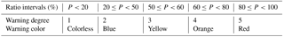
For the purposes of practical implementation of this forecasting model, P is divided into a series of reference intervals in Table 1; the occurrence probability of shallow landslides increases from the first to the fifth interval of P. Five grades of landslide warnings are defined accordingly and color-coded Table 1.

Table 1 Reference intervals for shallow-landslide forecasting based in probabilistic safety factor.

3 Probabilistic shallow-landslide forecasting method at regional scale

3.1 Gathering basic data necessary for landslide forecasting

Topography is the main factor in shallow landslides. Nowadays, obtaining a digital elevation model (DEM) of precision adequate for regional-scale forecasting is straightforward. The DEM of the study zone is resampled into pixels with dimensions according to the extension of the area. The parameters required to calculate the ratio P for each pixel from the array of safety factors $F_{{\mathrm{s}}_i}$ from a series of randomly extracted [c_i, φ_i] are identified in Eq. (1). In this case matrix suction, which is associated with the soil water content, should be identified by hydrological process simulation.

The key data necessary for the hydrological process simulation include the spatial distribution of precipitation, land use, soil type and normalized difference vegetation index (NDVI). Precipitation data with the same solution of the DEM can be obtained by resampling rainfall prediction from Doppler radar supplied by meteorological bureaus. Land use, soil type and soil depth can be obtained from corresponding databases, all of which should be transformed into grid data with the same solution of DEM. Other data necessary for stability calculations are slope angle for each pixel, parameters from the soil water characteristic curve (α, m, n) and soil mechanical parameters. Slope angles can be derived from DEM using spatial analyst tools; parameters (α, m, and n) of the soil water characteristic curve are derived from the different soil types within the pixel.

Regarding the identification of soil mechanical parameters (cohesion force and internal friction angle), a relatively reliable way, such as field sampling or soil-texture-based methods, should be used to assign an initial basic value to each pixel. Although these values include high uncertainty levels, they are used only as reference values while setting intervals of c=U(c_min, c_max) and φ=U(φ_min, φ_max) (Raia et al., 2014). In this study, the lithology of the study zone is derived from a geological map, and the mechanical parameters (cohesion force and internal friction angle) of the corresponding lithology are identified using a rock mechanics handbook (Ye et al., 1991). Finally the data are assigned to each pixel using the grid cells of the DEM as a reference.

From Eqs. (3) and (4), it is necessary to identify the lower and upper border of intervals of the soil mechanical parameters. However, the exact values for lower (c_min and φ_min) and upper (c_max and φ_max) limits are very difficult to determine. From currently published papers, there is no known theoretical or experimental method to solve this issue. Raia et al. (2014) used variations of 1, 10 and 100 % around the values of cohesion force and internal friction angle (from field tests) to get several intervals, showing that the forecasting effectiveness is significantly improved by using large variations. Consequently, this method applies a variation of 100 % around the mean value of these parameters for each pixel to set the corresponding lower and upper borders as follows:

$$\begin{array}{}\text{(7)}& {\displaystyle }& {\displaystyle }{c}_{\text{random}}\in [\mathrm{0.5}\times c_{\text{origin}},\mathrm{2}\times c_{\text{origin}}],\text{(8)}& {\displaystyle }& {\displaystyle }{\mathit{\phi }}_{\text{random}}\in [\mathrm{0.5}\times {\mathit{\phi }}_{\text{origin}},\mathrm{2}\times {\mathit{\phi }}_{\text{origin}}],\end{array}$$

where c_random and φ_random are the randomly extracted cohesion forces and internal friction angles, and c_origin and φ_origin are the mean value of each pixel (in this case from the rock mechanics handbook; Ye et al., 1991).

3.2 Pixel level hydrological process simulation

The simulation of hydrological processes including rainfall interception, infiltration and evapotranspiration is extremely complicate. However, rainfall infiltration is the key factor in the distribution of soil water content in the underlying surface, which simplifies the analysis. In the southwestern region of China slopes are almost unsaturated before the rainy season due to characteristic distribution of rainfall influenced by the monsoon (Zhang et al., 2014b). The infiltration process in the vertical direction in unsaturated soil mass can be described by the 1-D Richards equation (1931):

$$\begin{array}{}\text{(9)}& {\displaystyle \frac{\partial \mathit{\theta }}{\partial t}}={\displaystyle \frac{\partial }{\partial z}}\left[D\left(\mathit{\theta }\right){\displaystyle \frac{\partial \mathit{\theta }}{\partial z}}\right]-{\displaystyle \frac{\partial K\left(\mathit{\theta }\right)}{\partial \mathit{\theta }}},\end{array}$$

where θ is soil water content; $D\left(\mathit{\theta }\right)=K\left(\mathit{\theta }\right)/(\text{d}\mathit{\theta }/\text{d}\mathit{\psi })$ is the hydraulic diffusivity; ψ is the suction of unsaturated soil; z represents the soil depth, which is positive along the soil depth and has the topsoil as the origin point; and K(θ) is the hydraulic conductivity. The matrix suction is the dominant external force to drive the water movement in unsaturated soil mass, which can be calculated from Eq. (2).

Infiltration upper border: if the topsoil is unsaturated, it has a strong infiltration capacity (Lei et al., 1988). Then, while the rainfall intensity is less than the infiltration capacity of the topsoil, all precipitation will infiltrate into the topsoil without any runoff. In this scenario, the infiltration border is governed by Eq. (10):

$$\begin{array}{}\text{(10)}& -D\left(\mathit{\theta }\right){\displaystyle \frac{\partial \mathit{\theta }}{\partial z}}+K\left(\mathit{\theta }\right)=R\left(t\right),t>\mathrm{0},z=\mathrm{0},\end{array}$$

where R(t) is the rainfall intensity at time t. Here, the part of precipitation that exceeds the capacity of infiltration of the topsoil will transform into runoff (no water storage above topsoil). In this case the topsoil of a pixel is considered saturated. Thus, Eq. (10), which governs the upper border of infiltration, is transformed into the equation of θ=θ_s (Lei et al., 1988). There θ_s is the saturated moisture corresponding to the soil type.

Infiltration bottom border: it has been experimentally demonstrated that the soil water content beyond a soil depth of 40 cm is barely influenced by rainfall infiltration (Cui et al., 2003). Consequently a region with a groundwater level near the surface of the soil has hydrological characteristics in which rainfall infiltration can hardly induce any groundwater level variation. In this case, it is reasonable to ignore the water exchange process between the lower boundary and groundwater (Zhang et al., 2015).

An implicit finite difference method is used for discretization of the 1-D differential equation of water movement. The calculation time t is segmented into several intervals with the same time gap t, and the soil depth L of each pixel is segmented into soil layers (each layer is named of i numbers) with the same depth z.

Identifying the initial soil water content is an important issue during the hydrological simulation process. However, this value cannot be directly determined at any given time for a large region due to complex rainfall infiltration and evapotranspiration interactions. In the case of southwestern China, the winter is generally a relatively dry season; thus the soil water content value of the topsoil is very low, close to the residual water content of the soil type (Zhang et al., 2014b). This situation is exploited by setting the simulation time to start on 1 January of the forecasting year (driest month in winter), which allows the use of the residual water content corresponding to the soil type and the initial value of the topsoil water content. Measured meteorological data from 1 January are then fed to the simulation, which allows for a relatively accurate initial value of soil water content for the landslide forecasting. Each simulation step also takes into account the rainfall interception and evapotranspiration processes by means of the algorithm of the distributed hydrological model GBHM (Yang et al., 2002).

After the hydrological simulation process identifies the initial soil water content of each pixel, the simulation focuses on the extraction of key hydrological parameters (soil water content and matrix suction) necessary for the stability calculation of each pixel using the expected rainfall from Doppler radar forecasting. During this last stage in the simulation in which landslide forecasting is performed, the evapotranspiration processes is not considered since this period is typically short, with rainfalls, negligible sunshine and lower temperatures.

3.3 Probabilistic landslide forecasting at pixel level

During the forecasting stage, the hydrological parameters (soil water content and matrix suction) of each pixel in each forecasting step t are extracted via hydrological process simulation. Then the ratio P is computed for each pixel in several steps as follows: (1) H_s representing the instable soil depth in Eq. (1) is not equal to the soil depth L in Sect. 3.2 and cannot be identified in advance. We have to divide each pixel with a certain soil depth L into several soil layers in order to calculate the F_s using Eq. (1) layer by layer. When the calculated soil layer is the jth, the parameters H_s will be equal to the sum of all the soil layers above the jth layer (including the depth of the jth soil layer). As mentioned in Sect. 3.2, each pixel was divided into soil layer with the same depth. The matrix suction and soil water content are the important hydrological parameters to the stability analysis of the pixel which will be calculated and saved in each divided soil layer after the hydrological process simulation. So we adopt the same discretization rule during the stability analysis in order to easily extract these hydrological parameters. (2) The Monte Carlo method is used to extract the cohesion force and the internal friction angle n times from the corresponding intervals (c=U(c_min, c_max) and φ=U(φ_min, φ_max)) of each pixel. (3) The safety factor F_s of each divided layer within one pixel is calculated after each extraction, using the soil mechanical parameters and the hydrological parameters only related to time as inputs of Eq. (1); if the F_s of the jth layer is less than 1, then the calculation process within the pixel will stop. (4) Once the Monte Carlo process ends, the total times sum${}_{F_{\mathrm{s}}<\mathrm{1}}$ (a count of the number of occurrences satisfying the instability condition) is obtained, and the ratio P of F_s<1 is calculated using Eq. (6). (5) Finally the interval of Table 1 where ratio P is located according to its value is assigned to the pixel as the early-warning information to be broadcasted.

After completing this process for all pixels within the forecasting region, the whole calculation at time t is finished; meanwhile a map of landslide warning degrees in the forecasting region will be generated at the end of each forecasting step. Such maps can then be used by the forecasting bureau of the region to issue landslide warnings to hazard mitigation units and the public.

4 Verification of the probabilistic landslide forecasting model

4.1 Study zone

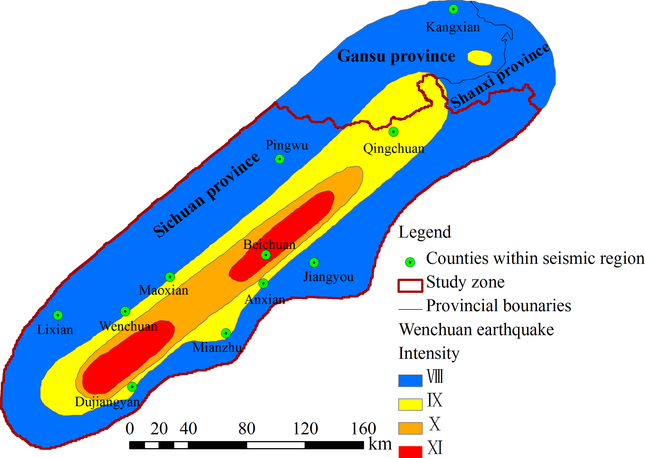
The Wenchuan earthquake region with an area of 3.14×10⁴ km² within Sichuan province, China, is chosen as the study zone in this study (Fig. 2). In this region, at 14:28 (Beijing time) on 12 May 2008, an M 8.0 earthquake occurred. Massive potentially unstable slopes were left after this earthquake, which are known to readily evolve into shallow landslides by rainfall infiltration (Zhang et al., 2016). The close relationship between rainfall and landslides in this region has been demonstrated by the short lag time of landslides and its strong correlation to rainfall time (Tang, 2010). The same study established that landslide events within the earthquake region are mainly in the form of shallow landslides (Tang, 2010). Tang (2010) also pointed out that shallow landslides will be active within the Wenchuan earthquake region at least for the next 10 years. Such conditions make this region ideal for implementation of shallow-landslide forecasting models.

Figure 2 Study zone and intensity distribution of Wenchuan earthquake.

4.2 Rainfall process and related landslide events used for testing

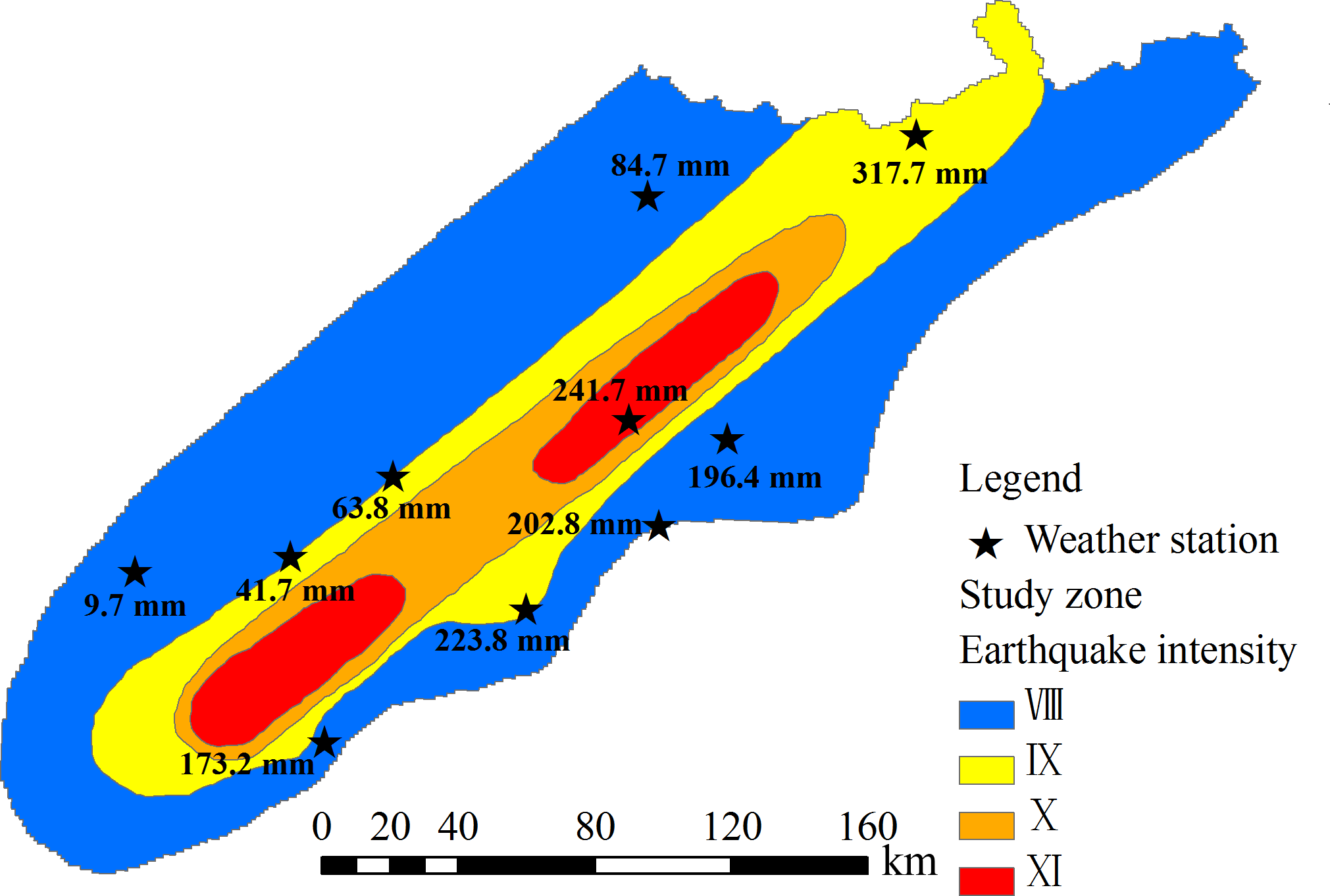
The chain of events in the Wenchuan earthquake area that ended in disastrous landslides in 9 July 2013 was chosen to evaluate the proposed landslide probabilistic forecasting method. These events started with heavy rainstorms in the area during the days from 1 to 8 July 2013. As the rainfall measured by the weather stations within the area shows (Fig. 3), the maximum accumulated precipitation during these days reached 317.7 mm, which is a key contributing factor for the landslide events of 9 July 2013.

Figure 3 Total rainfall from 1 to 7 July 2013.

On 9 July 2013, there was no evidence of decreasing rainfall intensity; on the contrary, all evidence suggested heavier rainfalls. Records from the rainfall forecasted by Doppler radar provided by the weather bureau of Sichuan province on that day predicted a maximum 24 h total precipitation within the earthquake region of up to 498 mm (Fig. 4). Accordingly, the Weather Bureau of Sichuan province published red-color warning signals (the highest alert degree) for some locations within the study region. On that day, 176 landslide events were reported within the study region (Fig. 4), leading to casualties and serious economic losses for local residents (Zhang et al., 2014b). This typical landslide disaster triggered by intense rainfall is ideal for evaluating the main aspects of the implementation of the proposed probabilistic landslide forecast model at regional scales.

Figure 4 Distribution of rainfall-induced landslides within Wenchuan earthquake region on 9 July 2013.

4.3 Gathering of basic data of study zone

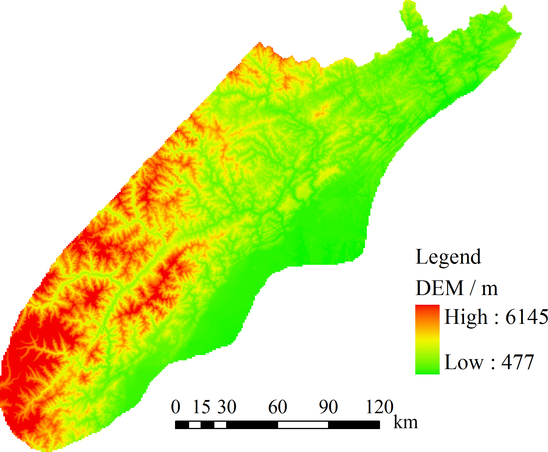
The topography of the study region (Fig. 5) was described by a DEM with 125×125 m resolution. This way, the study region was segmented into 6 965 505 pixels. A data matrix with 2576 rows and 2704 columns was created from the DEM and saved in text format. The basic data for hydrological process simulation and stability were resampled to correspond to the same resolution of the DEM and saved as text matrices with the same dimensions.

Figure 5 DEM of Wenchuan earthquake area.

Figure 6 Distributions of the leaf area index (LAI) within the study zone.

4.3.1 Data for hydrological process simulation

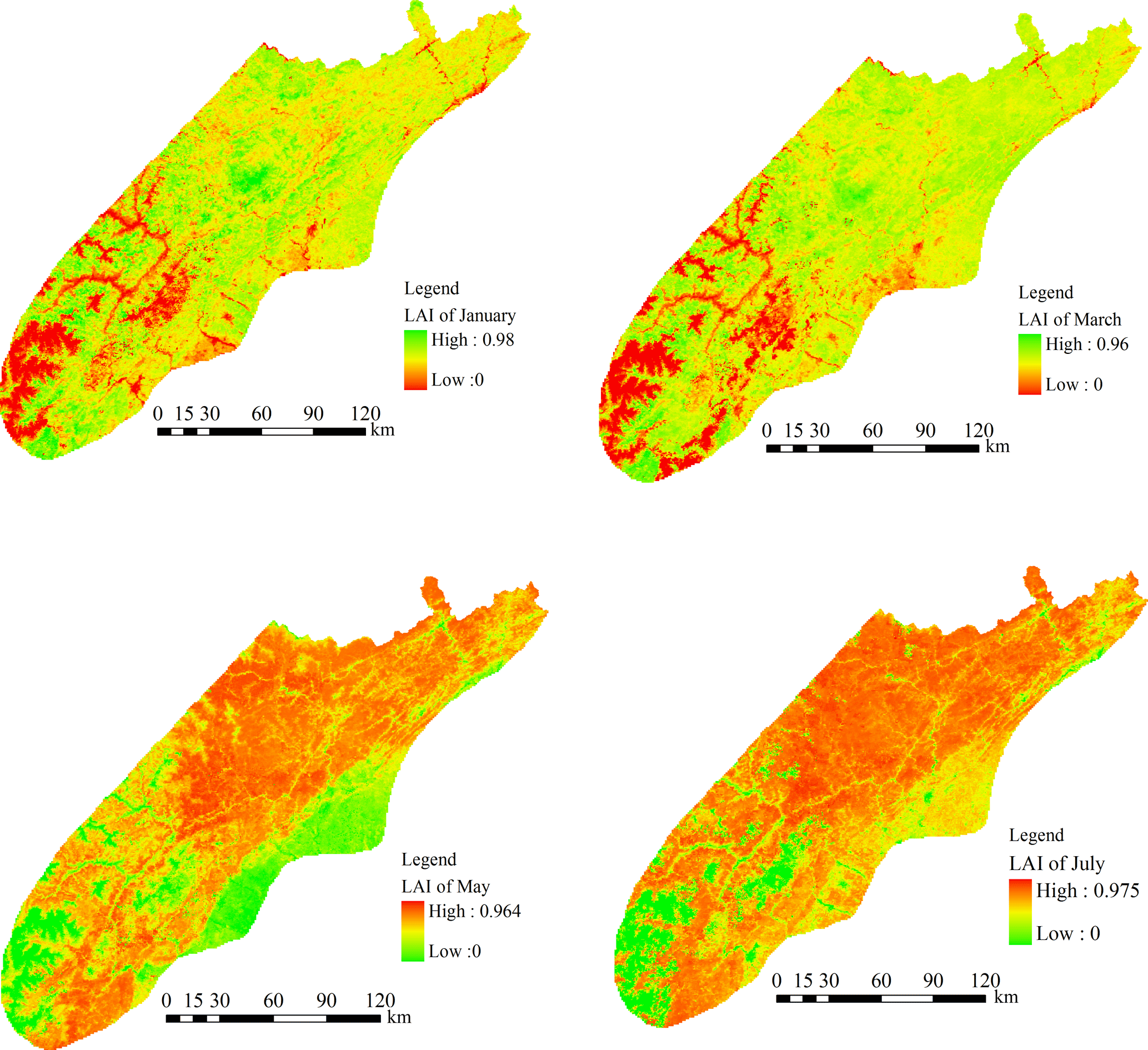
The process of rainfall interception due to vegetation influence within the study region is taken into account using NDVI values. Generally, the vegetation and thus the values of NDVI vary with the variation of land uses and seasons. In this case, NDVI values from the same region of the adjacent year are considered reasonably close, since the distribution of land uses within a region is relatively stable. The monthly NDVI distribution over the study region in the preceding year (2012) was used to adjust for canopy rainfall interception during the hydrological process simulation (Fig. 6).

Figure 7 Information of land uses and soil types within the study zone.

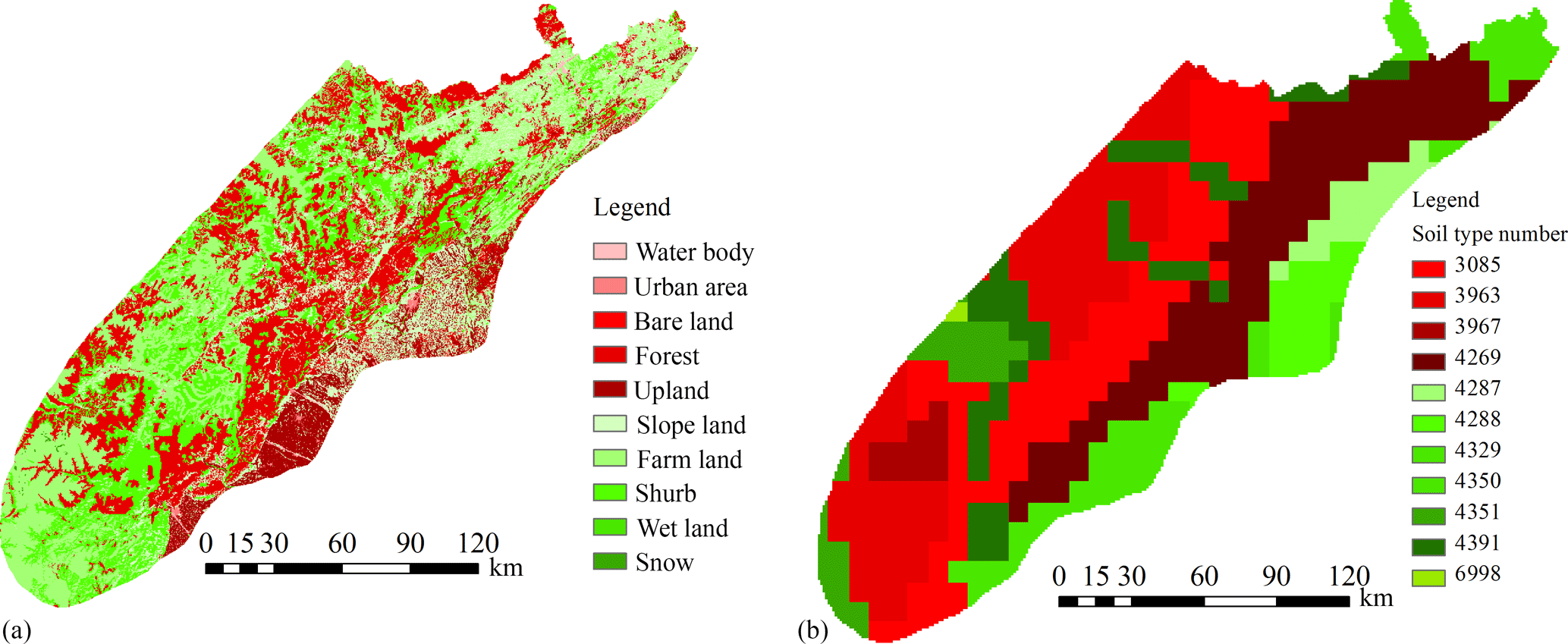
Other data required – such as land use (Fig. 7a), soil type (Fig. 7b), and soil depth for the Wenchuan earthquake region – was obtained from the FAO database (http://www.fao.org/geonetwork/srv/en/main.home). These data were processed using GIS functions so that they correspond to the pixels of the DEM.

Figure 8 Mechanical parameters of soil used for calculation of slope stability.

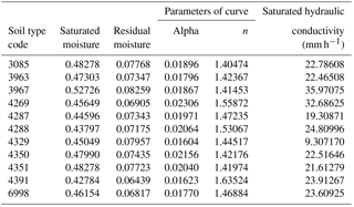
The physical parameters of the soil required for the simulation of rainfall infiltration in the vertical direction were determined by the land use and standard soil types within the study region. The soil thickness ranged from 1 to 4 m; soil depths of 1 m account for 44.1 % of the study area, while deeper soils cover the remaining 55.9 %. Each pixel was divided into 10 layers (along the soil depth in the vertical direction) during the hydrological process simulation and stability analysis. There are 10 soil types in the area (shown in Fig. 7b). Their relevant physical properties are listed in Table 2.

Table 2 Soil water parameters for hydrological simulation.

4.3.2 Data for calculation of slope stability

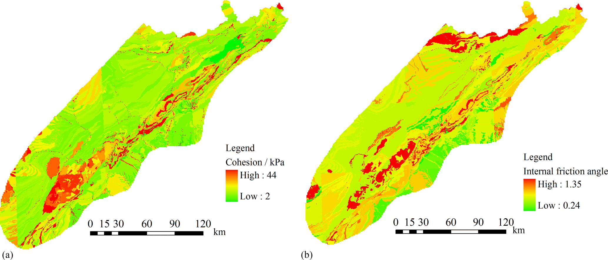
Eq. (1) indicates that matrix suction, cohesion force and internal friction angle are the key mechanical parameters influencing the slope stability. Simulation of the hydrological process is used to obtain the matrix suction of soil mass as a function of the soil water content as shown in Eq. (2). Cohesion forces and internal friction angles for each pixel updated from the old database (Liu et al., 2016) are determined according to the lithology map and the rock mechanical handbook (Fig. 8). The detailed process to obtain these data is as follows: each pixel will be firstly assigned the lithology attribution according to the lithology map, and then the rock mechanical handbook, which contains the mechanical parameters of all lithology, will be used to find the corresponding parameters of each pixel. These mechanical values are then used as a basic reference for constructing intervals of these parameters (c=U(c_min, c_max) and φ=U(φ_min, φ_max)) for each pixel.

4.4 Forecasting results

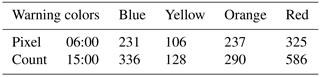
The landslide probability in the Wenchuan earthquake region on 9 July 2013 was calculated, along with color-coded warnings for each pixel according to Table 1. This forecast covered 24 time nodes (hourly forecasts) covering the whole day. Two representative time nodes (at 06:00 and 15:00) are chosen from the 24 h forecasting results for further analysis (Fig. 9). The detailed forecasting results are listed in Table 3. These details denote low variation in the forecast for these time nodes.

Table 3 Quantity of pixels with warning information.

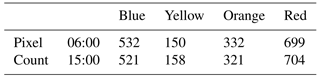
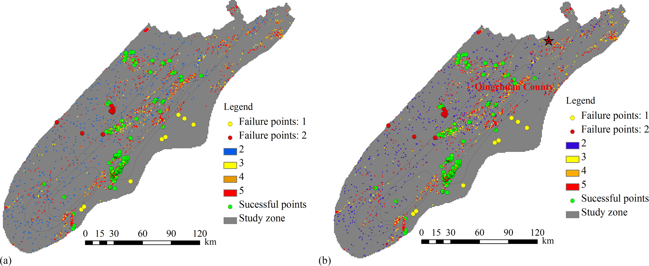
Figure 9 Landslide warning maps for Wenchuan earthquake region at two representative time nodes.

Figure 10 Initial conditions for landslide forecasting.

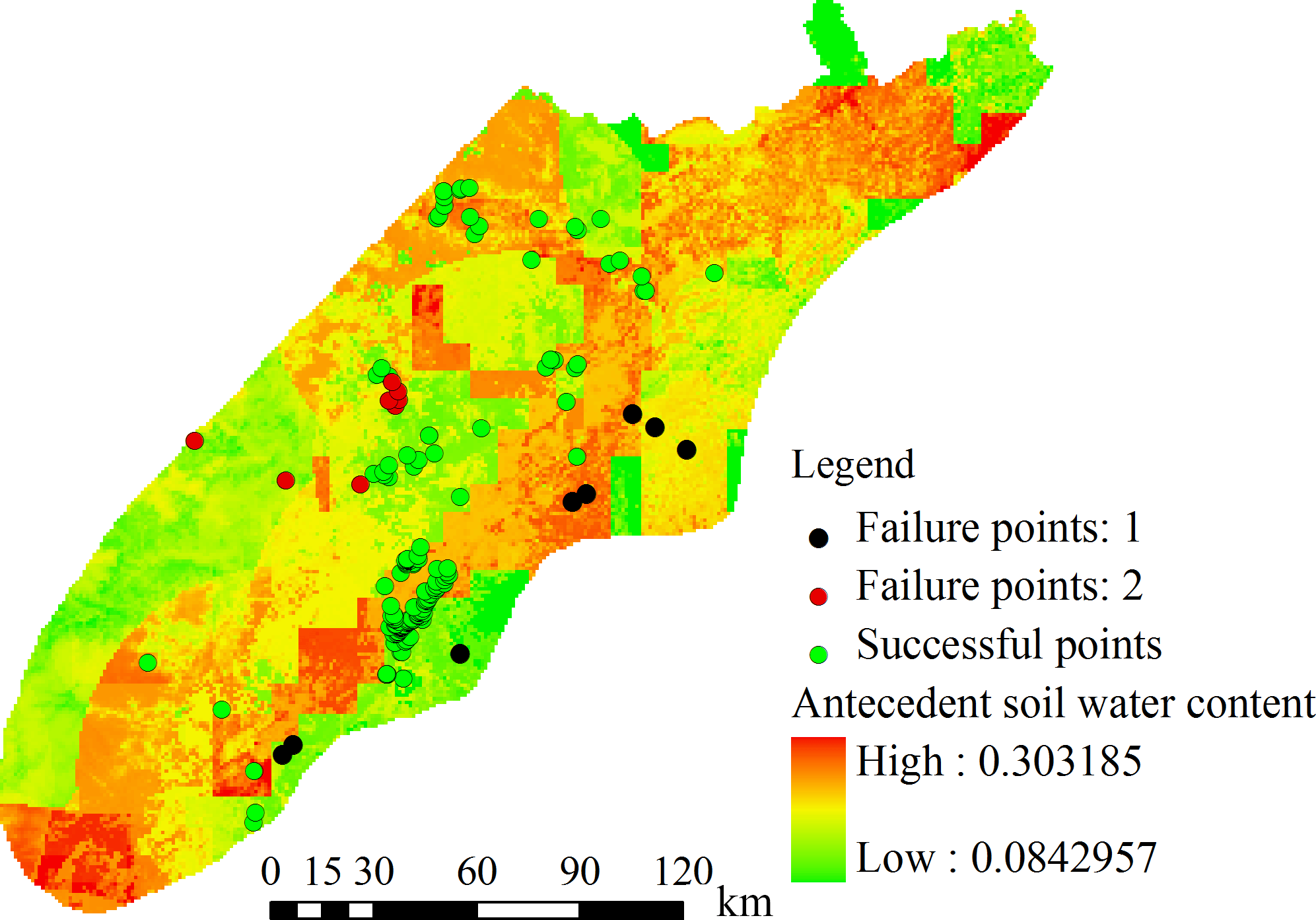
Figure 11 Forecasting results without considering the influence of the antecedent soil water content.

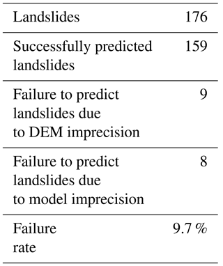
Colored points in Fig. 9 represent landslide disasters that occurred on 9 July 2013. Green points represent landslides located in pixels forecasted with a high degree of probability of landslides (orange–red); thus they are considered successfully forecasted or true positives (159 events). The other 17 events represented by yellow and red points denote landslide events in low-warning areas, which are considered as failed-forecasted landslides or false negatives. These numbers indicate a missing-prediction rate of the new proposed forecasting model of about 9.7 %.

Further analysis of these failures indicated that in some cases the maximum slope angle of the corresponding pixel reported by the DEM is less than 4^∘ (yellow points). Furthermore, four of these pixels have slope angles equal to 0 from the DEM. These small angles are for practical effect equal to flat terrain. In this scenario the probabilistic forecast model is unable to predict any unstable state, even during a more serious rainstorm. However, the real occurrence of landslide events at these locations indicates further analysis is necessary. In this case, the most probable cause of this situation is the generalization process associated with the resolution of the DEM. It is well known that increasing the size of the pixel tends to lower the estimated slope value, which in turn will raise the failure prediction rate of models with high dependence on accurate slope values. A straightforward solution to this problem is to further reduce the size of the pixel, which will in turn represent the real slope angle more accurately. This solution, however, will drastically increase the computing time. As reference, the current matrix dimensions of 2576×2704 (for 125 m pixel size) represent the limit for a regular workstation when the data are not partitioned.

There are still eight prediction failures (marked by red dots) left unexplained. These are considered to be related to other aspects of the probabilistic forecasting model and unaccounted-for uncertainties. Detailed forecasting information about the landslide events in this study is listed in Table 4.

Table 4 Detailed forecasting analysis.

The false-prediction (false-positive) rate for the probabilistic forecast model is high. Fig. 9 shows high-warning degrees concentrated around Guangyuan city and Qingchuan County (marked by the “red star” in Fig. 9b), where landslide events did not occur. Looking at Fig. 3, we see that the accumulative precipitation within Guangyuan during the days of 1 and 7 July was 317.7 mm according to the local weather station. This implies initial soil water contents in the region close to saturation levels just before the forecasting time. Additionally, the cumulative precipitation predicted from the Doppler radar reached more than 470 mm in Guangyuan. Under the action of such a combination of strong antecedent rainfall and forecasted rainfall, it is reasonable to expect a high concentration of landslides (forecasted by the probabilistic model with different warning colors). Although the measured rainfall data for 9 July were not available for this study, indirect information (absence of report of landslides and other phenomena associated with heavy rainfall, even with notable initial soil water content levels) indicates the real precipitation on 9 July was much smaller than forecasted from Doppler radar. Given the known tendency of Doppler radar forecasts to overestimate rainfall, it is reasonable to consider the precision of Doppler radar rainfall as a key factor influencing the high false-prediction rates of the proposed probabilistic forecasting model.

5 Discussions

The general rule for the evolution of a slope from stability to failure is that the failure probability should increase as the rainfall process continues since increasing soil water content will decrease the suction matrix. This rule implies a forecasting result at 15:00 with more unstable pixels than the result at 06:00. However, both of them are relatively close.

The distribution map of initial soil water content at 24:00 on 8 July, shown in Fig. 10, indicates significant effects of accumulated rainfall for landslide forecasting; the topsoil of some areas is even in saturated conditions (this means that only the topsoil was saturated rather than the whole soil layer). The total saturated pixels within study region total 532.

Under these initial conditions, the mechanism of the runoff–infiltration process indicates that a significant amount of precipitation will transform directly into runoff as the soil water content value of topsoil increases. In this case study, these high levels of initial soil water content attributed to strong antecedent rainfalls lead to a lower variation rate of soil water content at pixel level. In this scenario, the variation of soil water content tends be gentle even during long and intensive rain, while excess water contributes mainly to the runoff process. This chain of events may explain the lack of clear evolution in the forecast in this particular study.

To further confirm this analysis, a new hydrological simulation was run in which the antecedent precipitation is ignored. The initial soil water content of each pixel for landslide forecasting was directly assigned with the residual soil water value according to the corresponding soil type (assuming a completely dry soil). All other parameters, including predicted rainfall from Doppler radar, remained unchanged from the previous simulation. The forecast results at 06:00 and 15:00 under these new conditions are shown in Fig. 11 and Table 5. It is easy to observe differences between forecasting times, with the quantity of unstable pixels at 15:00 being larger than at 06:00 as expected. In this case, the low level of initial soil water content allows for a strong infiltration process in the topsoil, which in turn leads to high variation rates for soil water content in each pixel, reflected in the differences of forecasting aligned with the expected evolution of the slope failure process.

The above analysis not only explains why there is not a big difference between 06:00 and 15:00 forecasts during a high-intensity rainstorm. It also stresses the relevance of the initial soil water content (or the effective antecedent rainfall) for any physically based landslide forecast model. A reliable method to calculate the initial soil water content can significantly influence the results of landslide forecasting models.

Table 5 Quantity of pixels with warning information, without considering the influence of antecedent soil water content.

Another issue is that most published physical models for landslide forecast, such as the SLIP (Shallow Landslides Instability Prediction) and TRIGRS models (Montrasio et al., 2011; Tsai and Chiang, 2012), overestimate the probability of landslide occurrence at regional scales. This proposed physics-based probabilistic forecasting model is also affected by this problem. From the point of view of input parameters, three key factors can lead to this high false-prediction rate. (1) The soil mechanical parameters can only be obtained indirectly at regional scales, which greatly increases uncertainty. Consequently, it is impossible to guarantee the correspondence of the fixed mechanical values at pixel level with the actual values in nature, even using large intervals of soil mechanical parameters such as in this paper. Underestimating these values increases the probability of identifying the corresponding pixel as unstable, which contributes to high false-prediction rates. (2) The nature of DEM models implies that a pixel identified as unstable by a pixel-based forecasting model may not really represent an unstable slope in nature. A slope may contain several pixels of which only a few are unstable, or more likely at regional scales, a pixel may include several slopes. In this scenario isolated unstable pixels can contribute to high false-prediction rates. (3) The precision of short-term rainfall forecasting is the last factor that can contribute to high false-prediction rates. This is relevant in this study, in which rainfall forecasts from Doppler radar overestimated the expected rainfall in some areas.

6 Conclusions

The extreme complexity of the landslide formation process means that even physics-based forecasting models are unable to model the slope instability with 100 % of confidence. However, the uncertainty of some input variables (e.g., soil mechanical parameters) is responsible for a significant part of this situation. This research adopted a probabilistic approach to express this uncertainty using Monte Carlo simulation. A single parameter (the ratio P) was devised to couple the uncertain nature of input variables with shallow-landslide forecasting. Furthermore, a regional physics-based probabilistic shallow-landslide forecasting model was developed around this parameter. The proposed model does not eliminate uncertainty; it manages it by explicitly introducing it into the model expressing the forecast directly in probabilistic form. Our tests showed that this approach increases the forecast precision (true positives) in real conditions, which is cardinal to protecting the public from catastrophic consequences of shallow landslides and other associated disasters (such as debris flows).

It must be noted that the complexity of landslide forecasting is not limited to the uncertainty of physical soil properties; this research points to the initial soil water content as another key variable extremely difficult to identify accurately at regional scales. The model proposed in this paper implements a simulation of the hydrological processes occurring in the soil to estimate this value. Such simulation is time intensive, which is unfavorable for real-world applications. Future research should focus on efficient methods for identification of soil water content at regional scales, which is a difficult but worthy challenge.

The goal of developing this physics-based probabilistic forecasting model is to serve for regional landslide disaster mitigation. Detailed-resolution data, which in the case of DEMs are readily available, are not always straightforward solutions for better forecasting results at this scale. In this case higher DEM resolution will improve the efficiency of the model failure prediction rates at the individual pixel level due to better slope representation. However, it will also increase the time and resources required by the model to produce usable results. A balance point between pixel-level precision and operational efficiency is required for the proposed model in order to make it more suitable for regional operation.