the Creative Commons Attribution 4.0 License.
the Creative Commons Attribution 4.0 License.
 | 02 Oct 2018
Has fire policy decreased the return period of the largest wildfire events in France? A Bayesian assessment based on extreme value theory
Thomas Curt
Nicolas Eckert
Very large wildfires have high human, economic, and ecological impacts so that robust evaluation of their return period is crucial. Preventing such events is a major objective of the new fire policy set up in France in 1994, which is oriented towards fast and massive fire suppression. Whereas this policy is probably efficient for reducing the mean burned area (BA), its effect on the largest fires is still unknown. In this study, we make use of statistical extreme value theory (EVT) to compute return periods of very large BAs in southern France, for two distinct periods (1973 to 1994 and 1995 to 2016) and for three pyroclimatic regions characterized by specific fire activities. Bayesian inference and related predictive simulations are used to fairly evaluate related uncertainties. Results demonstrate that the BA corresponding to a return period of 5 years has actually significantly decreased, but that this is not the case for large return periods (e.g., 50 years). For example, in the most fire-prone region, which includes Corsica and Provence, the median 5-year return level decreased from 5000 to 2400 ha, while the median 50-year return level decreased only from 17 800 to 12 500 ha. This finding is coherent with the recent occurrence of conflagrations of large and intense fires clearly far beyond the suppression capacity of firemen. These fires may belong to a new generation of fires promoted by long-term fuel accumulation, urbanization into the wildland, and ongoing climate change. These findings may help adapt the operational system of fire prevention and suppression to ongoing changes. Also, the proposed methodology may be useful for other case studies worldwide.
- Article
(918 KB) - Full-text XML
- BibTeX
- EndNote


Wildfires are important hazards and a major ecological disturbance. In southern France, 2500 fires are reported each year over the recent period (1994 to 2016) and burn an average of approximately 12 000 ha (Curt and Frejaville, 2018). Burned area (BA) distribution is highly asymmetric with a large number of small fires and rarely large ones. However, if the largest fires (>100 ha) represent only 1 % of the total number of fires, they account for approximately 70 % of the total BA and they consume two-thirds of the total annual budget dedicated to civil protection against fire risk (Chatry et al., 2010; Curt and Frejaville, 2018). In addition, such large and destructive wildfires are likely to increase in southern Europe due to changes in climate and landscape (Bedia et al., 2014; Oliveira et al., 2014). As a consequence, establishing new tactics and strategies for a better prevention and preparedness to face large fires has become a centerpiece of the European fire policy (EFIMED, 2011; Moreira et al., 2011; Fernandes et al., 2013; Tedim et al., 2016). Indeed, wildfire hazards are unique because they are fought and suppressed in real time by firemen, at least in Europe where almost no fire propagates freely. Hence, the final BA depends upon the balance between environmental and socioeconomic drivers that favor fire enlargement (remote terrain, strong wind, connectivity, and management of fuels and landscapes by humans; see Fernandes et al., 2016) and the efficacy of suppression tactics (Lahaye et al., 2014).
For many geophysical variables and/or hazards such as rainfall, snowfall, or river discharge, protective measures are designed to withstand an event with a given small exceedance probability, i.e., an event that is generally much rarer than those already observed (Sharma et al., 2012). As a consequence, a robust evaluation of the return period of these extreme events is of the utmost importance to risk mitigation (Read and Vogel, 2015; Volpi et al., 2015). Concerning fires, this information can help each year to predetermine the size of the fire crews and of fire tactical means such as airplanes and trucks in each region, in order to support ground forces if extreme fire events occur (Lahaye et al., 2014). It may also help governmental agencies and reinsurance companies to evaluate the cost of future fires in the current context of ongoing changes in climate and landscapes (Malamud et al., 2005; EFIMED, 2011).
Yet, to date, estimating return levels (e.g., 100 ha, 1000 ha) of fires corresponding to large return periods (e.g., >10 years) is rarely carried out and few dedicated studies are available (Hernandez et al., 2015). For instance, in southern France, no such study exists although this region is fire-prone and comprises a vast array of human, economic, and ecological assets at risk (Curt et al., 2016). In the literature, wildfire quantiles corresponding to large return periods have been fitted using power-law distributions (Malamud and Turcotte, 1999; Ricotta et al., 2001; Malamud et al., 2005). Cumming (2001) applies a truncated exponential distribution. Reed and McKelvey (2002) apply a stochastic model for the spread and extinguishment of fires, which is used to illustrate the deviation of the upper tail from a simple power-law distribution. However, as for other geophysical variables, extreme value theory (EVT) should be preferred due to its strong mathematical groundings (Coles, 2001). Specifically, in the univariate case, the generalized extreme value (GEV) distribution, the generalized Pareto distribution (GPD), or the combination of the GEV distribution with a Poisson point process (PP) are the representations of interest (Moritz, 1997; Alvarado et al., 1998; Holmes et al., 2008; Jiang and Zhuang, 2011; Hernandez et al., 2015). Hence, Jiang and Zhuang (2011) apply different extreme value distributions to BA of Canadian forests and differentiate wildfires according to the type of forest (boreal vs. taiga) and the source of ignition (human-caused vs. lightning). Hernandez et al. (2015) apply the GEV distribution to BA and fire radiative powers obtained using remote-sensing techniques over a large box covering the Mediterranean Basin.
This work aims at computing the return periods of wildfire BA in southern France using EVT. Specifically, we question the efficiency of the new fire policy set up in 1994 to reduce the likelihood of very large wildfires. This policy has been based on improved prevention of fires, increased surveillance of forests, and a massive attack on all ignitions in order to prevent fire enlargement (Curt and Frejaville, 2018). Indeed, even if this policy is probably efficient for reducing the mean BA, its real effect on the largest fires is still unknown. To this aim, our EVT framework is adapted to our case study (Fréjaville and Curt, 2015) and is nonstationary in time, i.e., it considers two distinct periods (1973 to 1994, and 1995 to 2016), and is also non-stationary in space, to account for three distinguished pyroclimatic subregions. In addition, a Bayesian approach (e.g., Robert, 1994; Gelman et al., 2013) is used to assess uncertainties in return levels. The comparison of the results between the different time periods and regions is used to assess the significance of the differences (e.g., how significant are the changes in return levels between 1973–1994 and 1995–2016). We use BA from the Prométhée fire database as a surrogate for fire risk, based on the assumption that the largest fires generate the highest impacts and costs for suppression and are among the most devastative (Lahaye et al., 2018). Our final goal is to provide risk managers with crucial information on the future likelihood of very large fires in southern France.
2.1 Study area and pyroclimatic regions
This study covers an area of 80 500 km2 located in the southeast of France (Fig. 1). Figure 1a presents the main geographical regions, which can be classified as Mediterranean lowlands (Provence, Languedoc-Roussillon, Maritime Alps), hinterlands, and foothills (Southern Alps, Cévennes), and mountainous areas (the Alps, Corsica, Massif Central, and eastern Pyrénées), which corresponds to high elevations (>1000 m a.s.l.). Mediterranean areas have a fairly dry and warm climate (mean rainfall <700 mm yr−1 and temperature >13 ∘C) and, as a consequence, they are conducive to fire activity. The frequency of wildfires is smaller in hinterland and mountain areas due to a high mean rainfall (>700 mm yr−1) and medium temperatures (<13 ∘C). Strong and dry winds also increase the summer fire activity along the Mediterranean coastline (fuel dryness, larger fire rate of spread; Fréjaville and Curt, 2015).
This study area encompasses different bioclimates, different vegetation fuels, and different levels of human activity (which generate about 95 % of ignitions), leading to different fire activities. For this reason we define three main homogeneous subregions based on fire activity and bioclimatic variables, so-called pyroclimatic regions (PCr, adapted from Fréjaville and Curt, 2015, ; see Fig. 1c). PCr-1 contains most fire hot spots of maximal fire activity with many fires (notably the largest ones) and large amounts of BA. It includes Corsica, Provence, and the Maritime Alps and concerns 64 % of all fires and 67 % of the total BA in southern France. In addition, it contains 63 % of the largest fires (>100 ha) and 74 % of the total BA of these fires. This is due to the combination of high fire weather danger, medium to high fuel amount, and connectivity in the landscape (Curt et al., 2013) as well as a very high density of human-caused ignitions by negligence, by accident, or by intent (Curt et al., 2016). This region is undoubtedly prone to large fires, which occur mostly in summer. PCr-2 has medium to high fire activity and covers the Mediterranean hinterland and mid-elevation mountains. PCr-3 has low fire activity and few large fires. It corresponds to high mountains with a wet and cool climate.
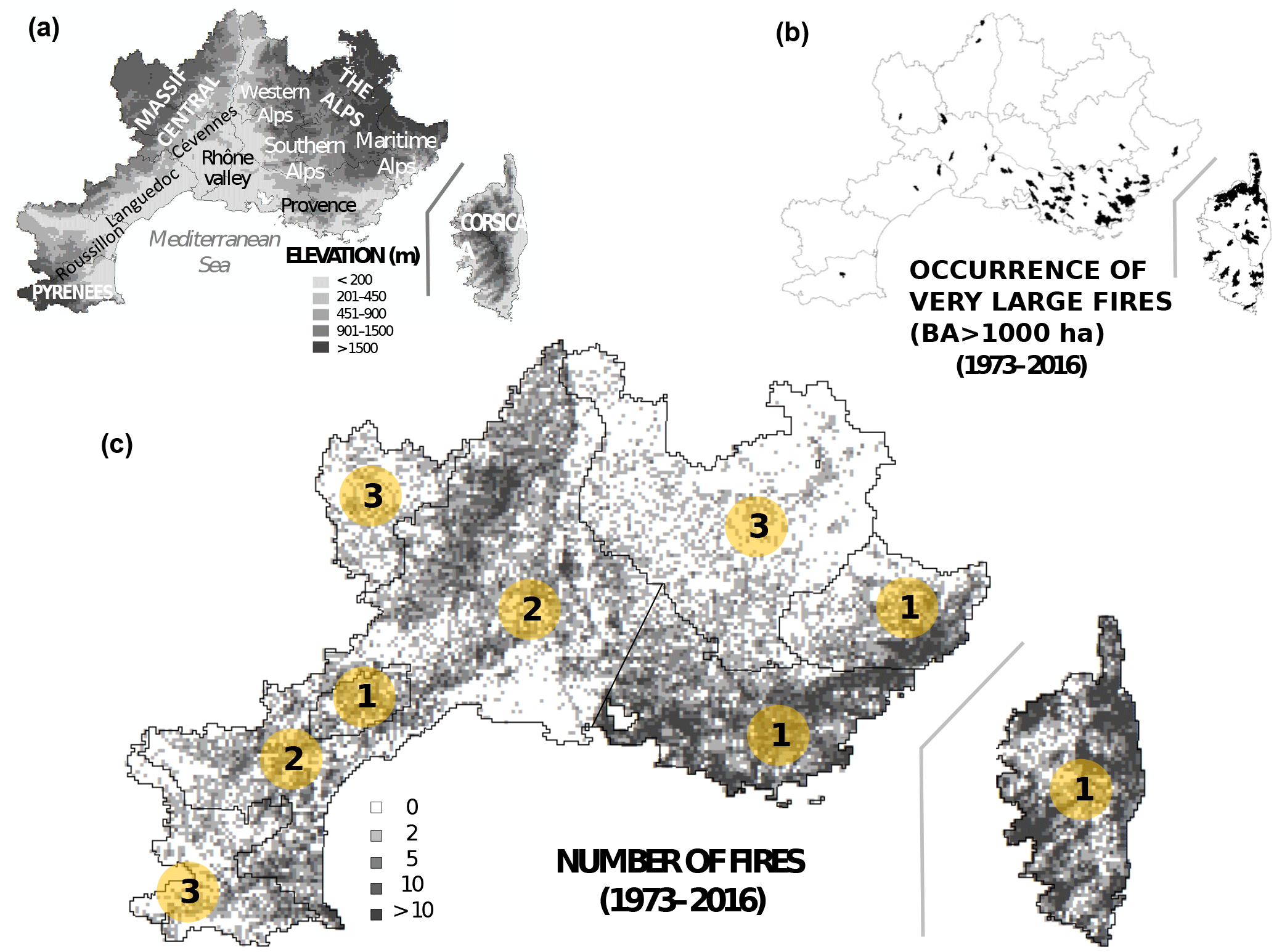
Figure 1Maps of the study area. (a) Geographical map. (b) Occurrence of very large fires (BA > 1000 ha.). (c) Density of the number of fires on a 2×2 km grid and location of the three pyroclimatic regions (numbered circles in yellow).
2.2 Fire database and BA thresholds
We use the national georeferenced fire database called Prométhée (Prométhée, 2016), which contains information on more than 106 000 wildfires. It corresponds to wildfire characteristics recorded by fire crews and foresters after each intervention from 1973 to 2016. Prométhée gives standardized information on each fire, including the day and hour of ignition, its location on a 2×2 km grid (with a total of 20 142 pixels), and the final BA in hectares.
Figure 2 presents the temporal evolution of the number of large fires (>100 ha) for each pyroclimatic region. Clearly, the fire activity is the highest in PCr-1, and PCr-3 has a limited number of large fires in comparison. From these time series, it is also evident that the fire policy set up in 1994 reduced the number of large fires in all regions.
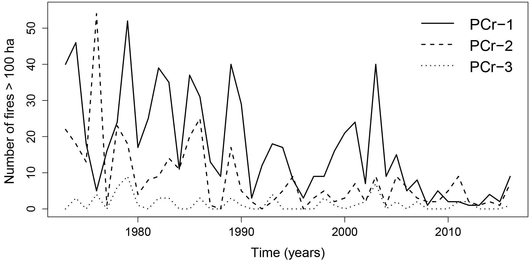
Figure 2Number of large fires (>100 ha) for each pyroclimatic region, as a function of time.
2.3 Extreme value theory
Extreme value theory (Coles, 2001) indicates that, under some mild conditions, the GEV distribution is the limiting distribution of maxima applied to very large blocks. In our case, the blocks correspond to the wildfire samples for each year. We assume that the wildfire samples are sufficiently large, so that annual maxima of BA can be considered to follow a GEV distribution. This has already been shown to be adequate in a very large number of applications, for example in hydrology (Katz et al., 2002; Papalexiou and Koutsoyiannis, 2013), finance and insurance (Embrechts et al., 1997), physics (Fortin and Clusel, 2015), mountain hazards (Gaume et al., 2013; Favier et al., 2016; Nicolet et al., 2016), or coastal engineering (Mazas and Hamm, 2011) to cite a few. The cumulative distribution function (cdf) of the GEV is
where is the set of parameters of the GEV distribution, μ∈IR the location parameter, σ>0 the scale parameter, and ξ∈IR the shape parameter. When ξ<0, the distribution has an upper tail and . When ξ=0, the distribution is unbounded. When ξ>0, the distribution has a lower bound () and when ξ increases, the distribution tail becomes heavier and very large values of x (here the BA) are more likely. The corresponding density function is
For the GEV distribution, the quantile Q(p|θ) corresponding to a probability p and a set of parameters θ is easily obtained:
For a return period T (e.g., T=20 years), the return level (e.g., 100 ha, 1000 ha) is thus expressed by .
2.4 Bayesian inference and Monte Carlo simulation
In this study, statistical inference is performed using Bayesian methods (see, e.g., monographs by Robert, 1994; Gelman et al., 2013). A Bayesian framework has several advantages compared to standard frequentist approaches. First, explicit a priori assumptions can be made about the parameters to estimate. Second, Bayesian methods provide a direct assessment of the uncertainty related to the parameter estimation. Generally, frequentist methods only provide confidence intervals based on theoretical results that hold true for very large samples (i.e., asymptotically). Third, in Bayesian methods, the uncertainty of a quantity of interest can be quantified by means of the predictive distribution. Here as well, frequentist methods provide similar theoretical results, which hold true under some restrictive conditions.
A Bayesian analysis combines the information in the data represented by the likelihood function with prior knowledge about the parameter. Parameter estimation is made through the posterior distribution, which is computed using Bayes' theorem
where Π(θ|D) is the posterior distribution of the GEV parameters θ, Π(D|θ) is the likelihood function, and Π(θ) is the prior distribution of θ. In this expression, it is assumed that the normalizing constant of the posterior distribution is unknown.
The likelihood function represents the conditional density of the data D, here the logarithms of the maximum BA, given the parameters θ, and describes the plausibility of observing the data D given θ. Here, we assume that the logarithm of these maxima are independently distributed (i.e., the maximum BA in a year y does not influence the maximum of the year y+1) and that they follow a GEV distribution. The likelihood is thus given by
where are the the logarithms of the maximum BA observed during N years. Here, following Hernandez et al. (2015), we choose to work with the logarithm of the maximum BA in order to solve scale issues. Indeed, raw BAs are measures of surface, i.e., two-dimensional data, and very large BA values (e.g., 1000 ha) are a lot larger than large BA values (e.g., 100 ha). This scale issue becomes obvious when the distribution of the raw BA is represented, this distribution being extremely skewed. As a consequence of these very skewed distributions, extreme value distributions with an infinite variance (i.e., when xi>0.5) are often obtained (see Moritz, 1997; Alvarado et al., 1998; Jiang and Zhuang, 2011) when they are applied to raw BA. Applying a log transformation to maximum BA is a convenient way to avoid this problem.
The prior distribution Π(θ) represents our a priori knowledge about the parameters θ. Here, we choose the following.
-
Location parameter : vague prior.
-
Scale parameter : vague prior.
-
Shape parameter . With this prior, ξ lies within and values greater than 0.3 are considered unlikely. Martins and Stedinger (2000) motivate this choice for several practical reasons. First, the variance of the GEV distribution is infinite when ξ>0.5 and the skewness coefficient is infinite when . Second, numerous geophysical applications show that, generally, ξ lies within this interval.
-
The joint prior distribution is ; i.e., the prior distributions are considered independent, which is usual in the absence of a priori information about some type of dependence among the GEV parameters (see, e.g., Coles, 2001, p. 174).
The posterior distribution Π(θ|D) can be sampled
using a Markov chain Monte Carlo (MCMC) algorithm
(Gilks et al., 1995; Robert and Casella, 2004). Here, we choose to apply the
Metropolis–Hastings algorithm (Metropolis et al., 1953) using the
function MCMCmetrop1R from the MCMCpack package in
R software (R Core Team, 2017). In this algorithm, candidates are
randomly generated from a proposal distribution and accepted as a new sample
according to an acceptance rate, which is computed using the posterior
distribution Π(θ|D). The main difficulty with the
Metropolis–Hastings algorithm is to find an adequate proposal distribution,
leading to a reasonable acceptance rate. In this work, the multivariate
normal proposal distribution is scaled using the covariance matrix of the
parameter estimates when the maximum-likelihood method is applied, using the
function fgev from the evd package in R. For each
estimation, we produce a burn-in sample size of 100 000, and the retained
sample used to represent the posterior distribution is M=10 000,
for which a thinning interval of 10 is applied in order to reduce the
autocorrelation inherent in MCMC chains produced with the Metropolis–Hastings
algorithm.
Draws from the posterior distribution Π(θ|D) can be used to estimate other unknown quantities. Specifically, the predictive distribution of a quantity , function of some arguments and depending on the GEV parameters θ, is expressed as (see Gelman et al., 2013, Eq. 1.4)
Hence, it fairly propagates the uncertainty related to parameter estimation on the quantities of interest. However, a closed expression of the predictive distribution can rarely be obtained, and it is often estimated using the draws from the posterior distribution:
where θ(i) is the ith draw from the posterior distribution. For example, the predictive distribution of a quantile (see Eq. 3) can be estimated by applying Eq. (7) with , i.e.,
Likewise, the predictive density of a maximum log-BA can be estimated with the expression , which can be used in turn to estimate specific probabilities, such as the exceedance probability of some critical log-BA xc. For example, the probability of having a BA x exceeding 10 000 ha in a year is obtained as
where is integrated over all values exceeding 10 000 ha, on the logarithm scale.
2.5 Measures of similarity between two distributions
Numerous statistical tests aim at testing an assumption of equality between two distributions (for example the test of Kolmogorov–Smirnov). These tests are adequate when two samples are compared and when we want to test if the sampling distributions can be considered equivalent. However, it must be noticed that these statistical tests are very powerful with large samples, which means that in this case, a small difference will be considered highly significant. As a result, comparing posterior distributions with these statistical tests generally results in a rejection of the assumption of equality, even when the distributions are very similar.
As an alternative, different measures have been proposed by statisticians in order to quantify the similarity between two distributions, or, in other words, how much two distributions overlap (e.g., Mahalanobis distance, Kullback–Leibler divergence). In this paper, we apply the Bhattacharyya coefficient (Bhattacharyya, 1946). This coefficient is easily normalized between 0 and 1, which facilitates its interpretation. Its expression is given by
where p(x) and q(x) are the probability density functions to be compared. We have , with BC=0 indicating that the distributions do not overlap and BC=1 indicating a complete similarity.
For the sake of comparison with statistical tests, when this coefficient is applied to two normal distributions N(0,1) and N(2,1) (shift of 2 standard deviations), it has a value of 0.61. Thus, two distributions can be considered similar when the Bhattacharyya coefficient exceeds 0.61. This reference value, while subjective, gives a more precise idea of the interpretation of the Bhattacharyya coefficient.
3.1 Relevance of the GEV distribution
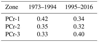
For each of the three regions PCr-1, PCr-2, and PCr-3, we collect the annual maxima of BA. Following the methodology described in Sect. 2, we fit a GEV distribution to the logarithm of annual maxima of BA for the periods 1973–1994 and 1995–2016 in order to assess the impact of the fire policy established in 1994. Table 1 presents the acceptance rates of the Metropolis–Hastings algorithm, which lie between 0.32 and 0.42. These acceptance rates are reasonable and correspond to common requirements. Indeed, acceptance rates between 0.23 and 0.5 are usually advised in order to obtain a fast convergence of the algorithm (Robert and Casella, 2004). A visual assessment of the traces of the sampled parameters did not reveal any convergence issue (results not shown).
Table 1Acceptance rates from the Metropolis–Hastings algorithm.
Taking the mean of the posterior distributions as point estimates, Fig. 3 shows the QQ plots of the fitted GEV distributions for each region and each period. This figure compares observed maxima and quantiles from the fitted GEV distribution corresponding to empirical probabilities of observed maxima. Points are close to the 1:1 line, which indicates that these adjustments are reasonable.
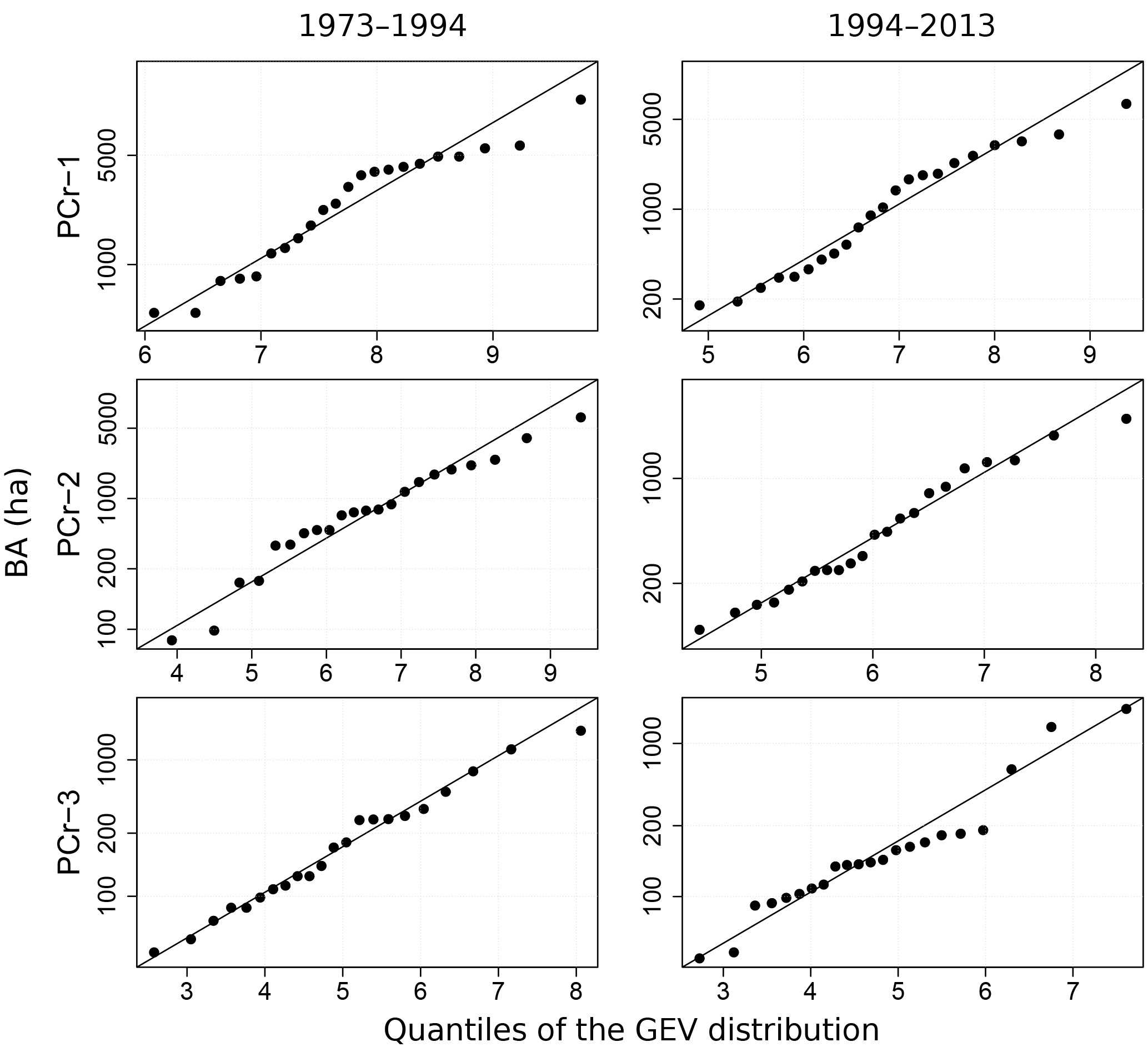
Figure 3QQ plot of the fitted GEV distributions for each region (PCr-1, PCr-2, and PCr-3) and each period (1973–1994 and 1995–2016). Point estimates of the GEV parameters are obtained as the mean of the posterior distributions. The BA (ha) is indicated on a log-scale.
3.2 Change in fire extremes before and after 1994
Posterior distribution estimates for the extreme value parameters μ, σ, and ξ, before and after 1994 and for each region, are shown in Fig. 4 and provide a direct assessment of the parameter uncertainty. Large differences are obtained for some parameters and some regions. For example, for region PCr-1, the location parameter μ has clearly decreased between the two periods, indicating that the fitted distribution has globally shifted toward smaller BAs after 1994. The scale parameter has decreased in regions PCr-2 and PCr-3 and slightly increased in region PCr-1. The shape parameter exhibits a slight increase in all regions. However, parameter uncertainty is large and the posterior distributions before and after 1994 overlap, which limits the interpretation of this increase.

Figure 4Comparison of posterior distribution of the GEV parameters, before (dashed line) and after 1994 (solid line): location parameter μ (log ha), scale σ parameter (log ha), and shape parameter ξ (dimensionless) for each region.
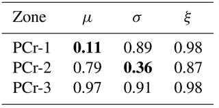
Table 2 quantifies these differences using the Bhattacharyya coefficient. As indicated above, this coefficient measures the similarity between two distributions. It is equal to 0 when the distributions do not overlap and 1 if they are identical. Table 2 indicates that, for region PCr-1, posterior distributions for μ before and after 1994 are clearly different, whereas they are roughly similar for the parameters σ and ξ, confirming the global shift of the distribution mentioned above. For region PCr-2, only σ has a significant change before and after 1994, while no difference is revealed for region PCr-3.
Table 2Bhattacharyya coefficients applied to posterior densities of the GEV parameters, before and after 1994, for each region. Bold values indicate coefficients below the reference value of 0.61.
For a return period T (e.g., T=100 years), the corresponding BA estimate is directly obtained, for a set of parameters θ, using Eq. 3. With the Bayesian approach, we can obtain the predictive distribution estimate of these return levels by applying Eq. (3) to all MCMC samples of parameters drawn from the posterior distribution (see Eq. 8).
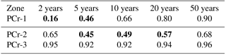
Figure 5 compares the predictive distributions of BA corresponding to return periods ranging from 2 years to 50 years, for periods before (in red) and after 1994 (in blue), for the three regions. For all regions, and particularly for region PCr-1, BAs corresponding to the smallest return periods (e.g., 2 years) have decreased, which demonstrates the efficiency of the fire policy established in 1994. However, for region PCr-1, the 90 % credible intervals overlap for higher return periods (e.g., 50 years). For this critical region, considering the large uncertainties associated with high return periods, no clear conclusion can be drawn in terms of decrease or increase in extreme return levels. The corresponding Bhattacharyya coefficients are given in Table 3 and indeed show that return levels have only changed significantly for return periods smaller than 10 years. For region PCr-2, the decrease in the return levels is more important, even for higher return periods (see Table 3). Finally, there is no noticeable change for region PCr-3.
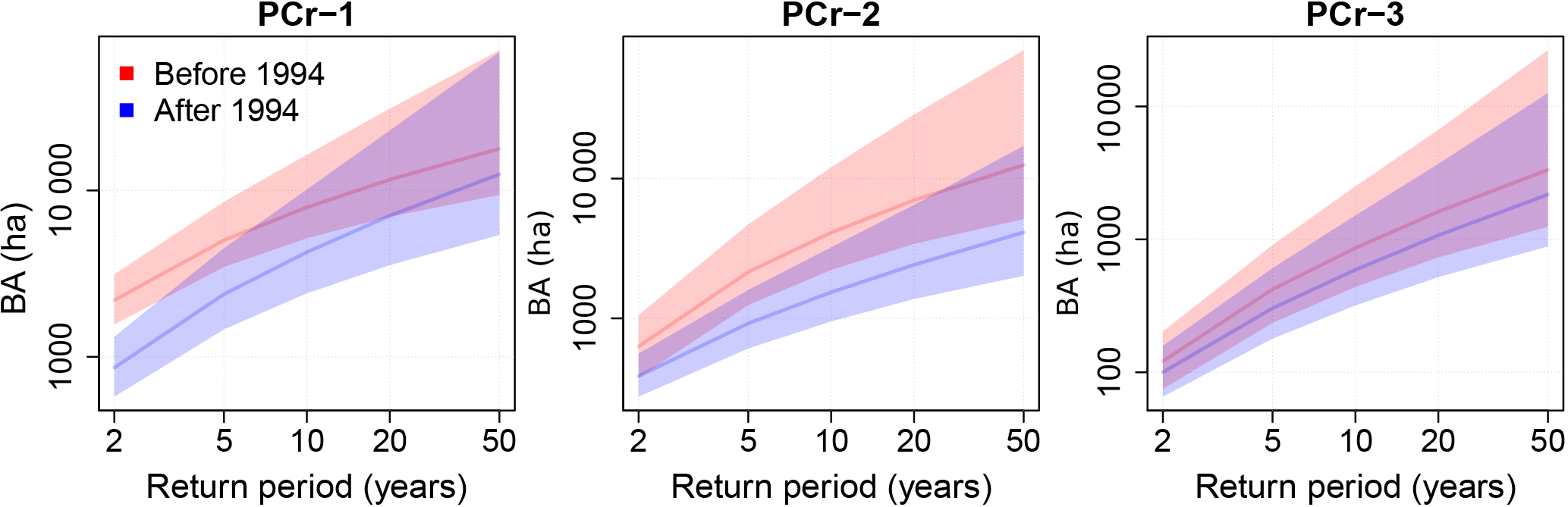
Figure 5Comparison of return levels, before and after 1994, for each region. The 90 % credible intervals are shown and median return levels are indicated in plain lines. BA (ha) is indicated on a log scale.
Table 3Bhattacharyya coefficients applied to different return levels, before and after 1994, for each region. Bold values indicate coefficients below the reference value of 0.61.
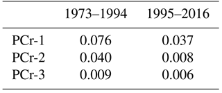
The probability of having very large fires (>10 000 ha) in a year is estimated using Eq. (9) and is given in Table 4. These estimates indicate a clear decrease in this probability before and after 1994 in regions PCr-1 (from 0.076 to 0.037) and PCr-2 (from 0.040 to 0.008). In PCr-2, the probability of having such large fires remains small (from 0.009 to 0.006).
Table 4Estimated probability of having very large fires (>10 000 ha) in a year, by area and for periods 1973–1994 and 1995–2016.
3.3 Return levels for the recent period (1995–2016)
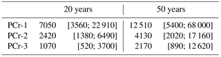
Table 5 reports the BA corresponding to high return periods (20 and 50 years), for the recent period 1995–2016. As an indicator of the central tendency of the predictive distributions of return levels, Table 5 reports the medians, i.e., the quantile 0.5. Median return levels correspond to BAs smaller than 5000 ha in regions PCr-2 and PCr-3. This is not the case in region PCr-1, for which BAs corresponding to 20- and 50-year return periods are very large (respectively 7050 and 12 510 ha). It can be seen that the 90 % credible interval corresponding to the 50-year return level of 12 510 ha in PCr-1 is very wide (from 5400 to 68 000 ha), which limits the interpretation of this estimate.
Table 5BA (ha) corresponding to different return periods (years), by area and for the recent period (1995–2016). Intervals between brackets indicate 90 % credible intervals of the corresponding return levels.
This study provides, for the first time, a model of fire return periods in southern France, taking into account the nonstationary nature of fire activity in space and time. EVT provides arguments in favor of the application of extreme value distributions (Coles, 2001). We show that the GEV distribution adequately fits the annual maxima of BA for each region and each period. In addition, we properly evaluate the uncertainty related to high return level using a Bayesian approach to estimate the parameters of the GEV distribution. As a result, the significance of potential changes can be assessed.
It appears that very large fires (>10 000 ha) are currently rare but not improbable in region PCr-1 (probability of 0.037) and less likely in regions PCr-2 (probability of 0.008) and PCr-3 (probability of 0.006); see Table 4. Hence, a major finding of this study is that, despite the new suppression-oriented policy set up in 1994, very large fires can still occur in southern France, and especially in the regional hot spots of Corsica and Provence. Indeed, in region PCr-1, the distribution of maximum BA has globally shifted toward smaller values between the periods 1973–1994 and 1995–2016 (see Fig. 5), but the current distribution is also more skewed. As a consequence, the BA corresponding to a return period of 50 years has not significantly decreased.
These findings provide information for leveraging fire risk. In the most fire-prone areas of France (Corsica and Provence), it is less and less doubtful that several ongoing changes will create opportunities for extreme fire events, as in many European countries (Tedim et al., 2018). Indeed, a combination of climate change, fuel accumulation, and increasing human pressure on ignitions in urbanized areas is the root cause for a new generation of wildfires characterized by extreme behavior (Costa et al., 2011). These new types of devastative fires are increasingly observed in southern Europe, such as in Portugal in 2017 (the Pedrógão Grande megafire burned 45 000 ha in June, 2017, and resulted in 66 fatalities) or in France in 2016 and 2017. For example, the Rognac-Vitrolles fire burned 2700 ha (August, 2016) and destroyed 39 habitations and a school. A total of 560 trucks and 1800 firemen were necessary to suppress the fire. Many of those fires are beyond the present suppression capacity (Lahaye et al., 2018). They often display eruptive or erratic behaviors, and they are able to propagate through landscape mixes in the wildland–urban interfaces and in cultivated areas. Recent studies in southern France have shown that new combinations of prolonged droughts, heat waves, and windy periods lead to a higher frequency of such extreme fire events (Ruffault et al., 2016a, b, 2018). In areas prone to extreme wildfire events, maintaining the pre-positioning of firemen in the field and massive aerial and ground forces for suppression is necessary every year. However, this may not be sufficient to control all fires during certain periods of very high hazard. In this context, managing landscapes and fuels, limiting unwanted ignitions and the participation of the public in self-protection (i.e., tackling the root causes of fire risk) are key to leverage fire risk in the long term. Concerning other pyroclimatic regions where fire activity is lower, the probability of very large fires is more limited. In mid-elevation hinterland (PCr-2) and in mountains (PCr-3), only a dozen fires larger than 100 ha were recorded each year on average since the 1990s. The ongoing climate changes favor an extension of areas with high fire weather danger towards the north and in the mountains (Dupire et al., 2017), and the season favorable to fire activity becomes longer. However, ignitions remain limited and fuels are rarely fully dry. This limits the probability of having very large fires. In these regions, the aerial surveillance by air tackers has been increased in order to detect fires as soon as possible.
Finally, it must be remembered that, in this study, we use the occurrence and BA of very large fires as a surrogate for extreme fire danger because no reliable and exhaustive database provides information on the real impacts of fire. This deserves discussion. On average, the largest fires actually have huge impacts on humans (including fire crews) and the environment because they are likely to have an effect on a large number of assets (Fernandes et al., 2016). This is especially true along the Mediterranean coastline, which is densely populated, densely urbanized, and very attractive for tourists. In addition, the largest fires need high expenditure to be suppressed (Lahaye et al., 2018). In this context, BA is likely the most appropriate surrogate for extreme fire events. However, a perspective is to better estimate their impacts by comparing the pre- and post-fire biomass in ecosystems and by building databases dedicated to impacts on people and infrastructures.
Extreme fire events (i.e., very large fires generating high human, economic, and ecological damages) are a growing issue in southern Europe and almost worldwide. Extreme fire events have a disproportionate impact on the media and they challenge the suppression-oriented policies because they question our ability to control or prevent them in the long term. In France, firefighting accounts for two-thirds of the total budget but it cannot suppress all large fires, as demonstrated notably in 2003, 2016 and 2017 (Chatry et al., 2010). Many large fires are erratic, fast growing, or convective (Lahaye et al., 2018) and cannot be controlled by firemen. They may belong to a new generation of fires promoted by global changes (Costa et al., 2011), which cause most of the accidents or fatalities for fire crews. This study demonstrates that even if the fire policy established in 1994 in southern France is undoubtedly successful, changes for BA corresponding to large return periods appear barely significant. The 50-year BAs remain important, especially in region PCr-1 (>10 000 ha), which includes Corsica, Provence, and the Maritime Alps. In addition to visual assessments, we propose using the Bhattacharyya coefficient in order to provide a quantitative assessment of the changes and take into account the uncertainty in the estimates. Based on these results, we propose solutions for leveraging large fires in a sustainable way in the future. Also, the rigorous proposed methodology that combines extreme value analysis and Bayesian tools may be useful for other case studies worldwide.
The Prométhée fire database is freely available online (http://www.promethee.com, last access: 28 September 2018).
GE developed the methodology for data analysis, carried out the analysis, and produced the results (tables and figures). He wrote the main part of the manuscript. TC conceived the study, provided the data, and wrote Sect. 4 and most of the conclusion. NE contributed to the development of the methodology and to the manuscript.
The authors declare that they have no conflict of interest.
This article is part of the special issue “Spatial and temporal patterns of wildfires: models, theory, and reality”. It is a result of the conference EGU 2017, Vienna, Austria, 23–28 April 2017.
Irstea – UR ETGR is a member of Labex OSUG@2020. Irstea – RECOVER is a
member of Labex OT-MED.
Edited by: Mário
Pereira
Reviewed by: two anonymous referees
Alvarado, E., Sandberg, D. V., and Pickford, S. G.: Modeling Large Forest Fires as Extreme Events, Northwest Sci., 72, 66–75, 1998. a, b
Bedia, J., Herrera, S., Camia, A., Moreno, J. M., and Gutiérrez, J. M.: Forest fire danger projections in the Mediterranean using ENSEMBLES regional climate change scenarios, Climatic Change, 122, 185–199, https://doi.org/10.1007/s10584-013-1005-z, 2014. a
Bhattacharyya, A.: On a Measure of Divergence between Two Multinomial Populations, Sankhyā: The Indian Journal of Statistics, 7, 401–406, 1946. a
Chatry, C., Le Gallou, J., Le Quentrec, M., Lafitte, J., Laurens, D., Creuchet, D., and Grelu, J.: Rapport de la mission interministérielle “Changements climatiques et extension des zones sensibles aux feux de forêts”, National Report on Climate Change and the Extension of Fire Prone Areas in France, Rapport Min. Alimentation Agriculture Pêche no. 1796, Paris, Tech. rep., 2010. a, b
Coles, S.: An Introduction to Statistical Modeling of Extreme Values, Springer Series in Statistics, Springer-Verlag, London, 2001. a, b, c, d
Costa, P., Castellnou, M., Larranaga, A., Miralles, M., and Kraus, D.: Prevention of Large Wildfires using the Fire Types Concept, Tech. rep., EU Fire Paradox Publication, Barcelona, Spain, 83 pp., 2011. a, b
Cumming, S. G.: A parametric model of the fire-size distribution, Canadian J. Forest Res., 31, 1297–1303, https://doi.org/10.1139/x01-032, 2001. a
Curt, T. and Frejaville, T.: Wildfire Policy in Mediterranean France: How Far is it Efficient and Sustainable?, Risk Anal., 38, 472–488, https://doi.org/10.1111/risa.12855, 2018. a, b, c
Curt, T., Borgniet, L., and Bouillon, C.: Wildfire frequency varies with the size and shape of fuel types in southeastern France: Implications for environmental management, J. Environ. Manage., 117, 150–161, https://doi.org/10.1016/j.jenvman.2012.12.006, 2013. a
Curt, T., Fréjaville, T., and Lahaye, S.: Modelling the spatial patterns of ignition causes and fire regime features in southern France: implications for fire prevention policy, Int. J. Wildland Fire, 25, 785–796, https://doi.org/10.1071/WF15205, 2016. a, b
Dupire, S., Curt, T., and Bigot, S.: Spatio-temporal trends in fire weather in the French Alps, Sci. Total Environ., 595, 801–817, https://doi.org/10.1016/j.scitotenv.2017.04.027, 2017. a
EFIMED: Wildfire Prevention in the Mediterranean. A key issue to reduce the increasing risks of Mediterranean wildfires in the context of Climate Change, forêt méditerranéenne, XXXII, second Mediterranean Forest Week of Avignon, France, 2011. a, b
Embrechts, P., Klüppelberg, C., and Mikosch, T.: Modelling Extremal Events: for Insurance and Finance, Stochastic Modelling and Applied Probability, Springer-Verlag, Berlin, Heidelberg, 1997. a
Favier, P., Eckert, N., Faug, T., Bertrand, D., and Naaim, M.: Avalanche risk evaluation and protective dam optimal design using extreme value statistics, J. Glaciol., 62, 725–749, https://doi.org/10.1017/jog.2016.64, 2016. a
Fernandes, P. M., Davies, G., Ascoli, D., Fernandez, C., Moreira, F., Rigolot, E., Stoof, C. R., Vega, J. A., and Molina, D.: Prescribed burning in southern Europe: developing fire management in a dynamic landscape, Front. Ecol. Environ., 11, e4–e14, https://doi.org/10.1890/120298, 2013. a
Fernandes, P. M., Barros, A. M. G., Pinto, A., and Santos, J. A.: Characteristics and controls of extremely large wildfires in the western Mediterranean Basin, J. Geophys. Res.-Biogeo., 121, 2141–2157, https://doi.org/10.1002/2016JG003389, 2016. a, b
Fortin, J.-Y. and Clusel, M.: Applications of extreme value statistics in physics, J. Phys. A-Math. Theor., 48, 183001, https://doi.org/10.1088/1751-8113/48/18/183001, 2015. a
Fréjaville, T. and Curt, T.: Spatiotemporal patterns of changes in fire regime and climate: defining the pyroclimates of south-eastern France (Mediterranean Basin), Climatic Change, 129, 239–251, https://doi.org/10.1007/s10584-015-1332-3, 2015. a, b, c
Gaume, J., Eckert, N., Chambon, G., Naaim, M., and Bel, L.: Mapping extreme snowfalls in the French Alps using max-stable processes, Water Resour. Res., 49, 1079–1098, https://doi.org/10.1002/wrcr.20083, 2013. a
Gelman, A., Carlin, J. B., Stern, H. S., Dunson, D. B., Vehtari, A., and Rubin, D. B.: Bayesian Data Analysis, Third Edition, Chapman and Hall/CRC, Boca Raton, 2013. a, b, c
Gilks, W. R., Richardson, S., and Spiegelhalter, D.: Markov Chain Monte Carlo in Practice, CRC Press, 1995. a
Hernandez, C., Keribin, C., Drobinski, P., and Turquety, S.: Statistical modelling of wildfire size and intensity: a step toward meteorological forecasting of summer extreme fire risk, Ann. Geophys., 33, 1495–1506, https://doi.org/10.5194/angeo-33-1495-2015, 2015. a, b, c, d
Holmes, T. P., Huggett Jr., R. J., and Westerling, A. L.: Statistical Analysis of Large Wildfires, in: The Economics of Forest Disturbances, edited by: Holmes, T. P., Prestemon, J. P., and Abt, K. L., no. 79 in Forestry Sciences, Springer, the Netherlands, 59–77, https://doi.org/10.1007/978-1-4020-4370-3_4, 2008. a
Jiang, Y. and Zhuang, Q.: Extreme value analysis of wildfires in Canadian boreal forest ecosystems, Can. J. Forest Res., 41, 1836–1851, https://doi.org/10.1139/x11-102, 2011. a, b, c
Katz, R. W., Parlange, M. B., and Naveau, P.: Statistics of extremes in hydrology, Adv. Water Resour., 25, 1287–1304, https://doi.org/10.1016/S0309-1708(02)00056-8, 2002. a
Lahaye, S., Curt, T., Paradis, L., and Hély, C.: Classification of large wildfires in South-Eastern France to adapt suppression strategies, in: Advances in Forest Fire Research, chap. 3 – Fire Management, Imprensa da Universidade de Coimbra, 696–708, https://doi.org/10.14195/978-989-26-0884-6_78, 2014. a, b
Lahaye, S., Curt, T., Fréjaville, T., Sharples, J., Paradis, L., and Hély, C.: What are the drivers of dangerous fires in Mediterranean France?, Int. J. Wildland Fire, 27, 155–163, https://doi.org/10.1071/WF17087, 2018. a, b, c, d
Malamud, B. D. and Turcotte, D. L.: Self-Organized Criticality Applied to Natural Hazards, Nat. Hazards, 20, 93–116, https://doi.org/10.1023/A:1008014000515, 1999. a
Malamud, B. D., Millington, J. D. A., and Perry, G. L. W.: Characterizing wildfire regimes in the United States, P. Natl. Acad. Sci. USA, 102, 4694–4699, https://doi.org/10.1073/pnas.0500880102, 2005. a, b
Martins, E. S. and Stedinger, J. R.: Generalized maximum-likelihood generalized extreme-value quantile estimators for hydrologic data, Water Resour. Res., 36, 737–744, https://doi.org/10.1029/1999WR900330, 2000. a
Mazas, F. and Hamm, L.: A multi-distribution approach to POT methods for determining extreme wave heights, Coast. Eng., 58, 385–394, https://doi.org/10.1016/j.coastaleng.2010.12.003, 2011. a
Metropolis, N., Rosenbluth, A. W., Rosenbluth, M. N., Teller, A. H., and Teller, E.: Equation of State Calculations by Fast Computing Machines, J. Chem. Phys., 21, 1087–1092, https://doi.org/10.1063/1.1699114, 1953. a
Moreira, F., Viedma, O., Arianoutsou, M., Curt, T., Koutsias, N., Rigolot, E., Barbati, A., Corona, P., Vaz, P., Xanthopoulos, G., Mouillot, F., and Bilgili, E.: Landscape–wildfire interactions in southern Europe: implications for landscape management, J. Environ. Manage., 92, 2389–2402, https://doi.org/10.1016/j.jenvman.2011.06.028, 2011. a
Moritz, M. A.: Analyzing extreme disturbance events: fire in los padres national forest, Ecol. Appl., 7, 1252–1262, https://doi.org/10.1890/1051-0761(1997)007[1252:AEDEFI]2.0.CO;2, 1997. a, b
Nicolet, G., Eckert, N., Morin, S., and Blanchet, J.: Decreasing spatial dependence in extreme snowfall in the French Alps since 1958 under climate change, J. Geophys. Res.-Atmos., 121, 8297–8310, https://doi.org/10.1002/2016JD025427, 2016. a
Oliveira, S., Pereira, J. M. C., San-Miguel-Ayanz, J., and Lourenço, L.: Exploring the spatial patterns of fire density in Southern Europe using Geographically Weighted Regression, Appl. Geogr., 51, 143–157, https://doi.org/10.1016/j.apgeog.2014.04.002, 2014. a
Papalexiou, S. M. and Koutsoyiannis, D.: Battle of extreme value distributions: A global survey on extreme daily rainfall, Water Resour. Res., 49, 187–201, https://doi.org/10.1029/2012WR012557, 2013. a
Prométhée: La banque de données sur les incendies de forêts en région Méditerranéenne en France, The French fire database, available at: http://www.promethee.com/ (last access: 25 September 2018), 2016. a
R Core Team: R: A language and environment for statistical computing, available at: https://www.r-project.org/ (last access: 25 September 2018), 2017. a
Read, L. K. and Vogel, R. M.: Reliability, return periods, and risk under nonstationarity, Water Resour. Res., 51, 6381–6398, https://doi.org/10.1002/2015WR017089, 2015. a
Reed, W. J. and McKelvey, K. S.: Power-law behaviour and parametric models for the size-distribution of forest fires, Ecol. Model., 150, 239–254, https://doi.org/10.1016/S0304-3800(01)00483-5, 2002. a
Ricotta, C., Arianoutsou, M., Diaz-Delgado, R., Duguy, B., Lloret, F., Maroudi, E., Mazzoleni, S., Manuel Moreno, J., Rambal, S., Vallejo, R., and Vázquez, A.: Self-organized criticality of wildfires ecologically revisited, Ecol. Model., 141, 307–311, https://doi.org/10.1016/S0304-3800(01)00272-1, 2001. a
Robert, C.: The Bayesian Choice: A Decision-Theoretic Motivation, Springer Texts in Statistics, Springer-Verlag, New York, 1994. a, b
Robert, C. and Casella, G.: Monte Carlo Statistical Methods, Springer Texts in Statistics, 2nd edition, Springer-Verlag, New-York, 2004. a, b
Ruffault, J., Moron, V., Trigo, R. M., and Curt, T.: Objective identification of multiple large fire climatologies: an application to a Mediterranean ecosystem, Environ. Res. Lett., 11, 075006, https://doi.org/10.1088/1748-9326/11/7/075006, 2016a. a
Ruffault J., Moron V., Trigo R. M., and Curt T.: Daily synoptic conditions associated with large fire occurrence in Mediterranean France: evidence for a wind-driven fire regime, Int. J. Climatol., 37, 524–533, https://doi.org/10.1002/joc.4680, 2016b. a
Ruffault, J., Curt, T., Martin-StPaul, N. K., Moron, V., and Trigo, R. M.: Extreme wildfire events are linked to global-change-type droughts in the northern Mediterranean, Nat. Hazards Earth Syst. Sci., 18, 847–856, https://doi.org/10.5194/nhess-18-847-2018, 2018. a
Sharma, A. S., Bunde, A., Dimri, V. P., and Baker, D. N., (Eds.): Extreme Events and Natural Hazards: The Complexity Perspective, American Geophysical Union, Washington, DC, 1st edn., 2012. a
Tedim, F., Leone, V., and Xanthopoulos, G.: A wildfire risk management concept based on a social-ecological approach in the European Union: Fire Smart Territory, Int. J. Disast. Risk Re., 18, 138–153, https://doi.org/10.1016/j.ijdrr.2016.06.005, 2016. a
Tedim, F., Leone, V., Amraoui, M., Bouillon, C., Coughlan, M. R., Delogu, G. M., Fernandes, P. M., Ferreira, C., McCaffrey, S., McGee, T. K., Parente, J., Paton, D., Pereira, M. G., Ribeiro, L. M., Viegas, D. X., and Xanthopoulos, G.: Defining Extreme Wildfire Events: Difficulties, Challenges, and Impacts, Fire, 1, 9. pp., https://doi.org/10.3390/fire1010009, 2018. a
Volpi, E., Fiori, A., Grimaldi, S., Lombardo, F., and Koutsoyiannis, D.: One hundred years of return period: Strengths and limitations, Water Resour. Res., 51, 8570–8585, https://doi.org/10.1002/2015WR017820, 2015. a