Characterizing severe weather potential in synoptically weakly forced thunderstorm environments

Weakly forced thunderstorms (WFTs), short-lived convection forming in synoptically quiescent regimes, are a contemporary forecasting challenge. The convective environments that support severe WFTs are often similar to those that yield only non-severe WFTs and, additionally, only a small proportion of individual WFTs will ultimately produce severe weather. The purpose of this study is to better characterize the relative severe weather potential in these settings as a function of the convective environment. Thirty-one near-storm convective parameters for > 200 000 WFTs in the Southeastern United States are calculated from a high-resolution numerical forecasting model, the Rapid Refresh (RAP). For each parameter, the relative odds of WFT days with at least one severe weather event is assessed along a moving threshold. Parameters (and the values of them) that reliably separate severe-weather-supporting from non-severe WFT days are highlighted.

Only two convective parameters, vertical totals (VTs) and total totals (TTs), appreciably differentiate severe-wind-supporting and severe-hail-supporting days from non-severe WFT days. When VTs exceeded values between 24.6 and 25.1 ^∘C or TTs between 46.5 and 47.3 ^∘C, odds of severe-wind days were roughly 5× greater. Meanwhile, odds of severe-hail days became roughly 10× greater when VTs exceeded 24.4–26.0 ^∘C or TTs exceeded 46.3–49.2 ^∘C. The stronger performance of VT and TT is partly attributed to the more accurate representation of these parameters in the numerical model. Under-reporting of severe weather and model error are posited to exacerbate the forecasting challenge by obscuring the subtle convective environmental differences enhancing storm severity.

1 Introduction

Weakly forced thunderstorms (WFTs), convection forming in synoptically benign, weakly sheared environments, are a dual forecasting challenge. Not only is the exact location and time of convective initiation difficult to predict, but, once present, the successful differentiation of severe WFTs from their benign counterparts is equally demanding. Consequently, severe weather warnings issued on WFTs in the US are less accurate than more organized storm modes, such as squall lines and supercells (Guillot et al., 2008). American operational meteorologists have coined these severe WFTs “pulse thunderstorms” because the surge of the updraft that produces the severe weather occurs in a brief “pulse” (Miller and Mote, 2017). The United States National Weather Service defines “severe weather” as any of the following: winds ≥ 26 m s⁻¹, hail ≥ 2.54 cm in diameter, or a tornado.

Environments thought to support pulse thunderstorms are typically characterized by weak vertical wind shear and strong convective available potential energy (CAPE). However, not all weak-shear, high-CAPE environments facilitate pulse thunderstorms, nor are all pulse thunderstorms confined to environments with the weakest shear and/or strongest instability. The result is a low signal-to-noise ratio (SNR) which obstructs the reliable discernment of pulse-supporting environments. The SNR is a common discussion point in climate variability research, where it often describes the relative magnitudes of a climate change trend (i.e., the signal) vs. interannual variability (i.e., the noise) (e.g., Hamlington et al., 2010; Sutton and Hodson, 2007; Trenberth, 1984). In our context, the “signal” refers to the true difference between the large-scale convective environments that support severe weather and those that do not. Meanwhile, the “noise” represents the many processes than might cause storms to produce (not produce) severe weather in an environment where it was not expected (expected). Cell interactions, stabilization from prior convection, surface convergence, locally enhanced shear, and model error, for example, can act as noise in the operational setting.

Prior research directed at pulse thunderstorms is limited, and work has not typically included a representative proportion of non-severe WFTs in their samples (Atkins and Wakimoto, 1991; Cerniglia and Snyder, 2002). If the sample contains too many pulse thunderstorms, the SNR may be artificially bolstered, results overstated, and the potential reliability in an operational setting diminished. For instance, in a meta-analysis of studies pertaining to new lightning-based storm warning techniques, Murphy (2017) found that the studies' reported false alarms ratios were directly proportional to the fraction of non-severe storms contained in the sample. Samples that included a realistic ratio of severe to non-severe storms demonstrated the weakest skill scores.

Most research considering pulse thunderstorms in the Southeastern US has typically focused on one of its primary severe weather mechanisms: the wet microburst. Severe wet microbursts generally occur in atmospheres characterized by a deep moist layer extending from the surface to 4–5 $\mathrm{km}\mathrm{a}.\mathrm{g}.\mathrm{l}.$ (Johns and Doswell, 1992). Above the moist layer lies a mid-level dry layer with lower equivalent potential temperature values (θ_e). In wet microburst environments, the difference between the maximum θ_e observed just above the surface and the minimum θ_e aloft exceeded 20 K, whereas non-microburst-producing thunderstorm days had differences less than 13 K (Atkins and Wakimoto, 1991; Roberts and Wilson, 1989; Stewart, 1991; Wheeler and Spratt, 1995). However, Atkins and Wakimoto (1991) examined only 14 microburst days vs. 3 non-microburst days. Adding to the uncertainty, James and Markowski (2010) challenged the role of mid-level dry air in severe weather production. The results of their cloud-scale modeling experiment indicated that, for all but the highest instabilities tested, drier mid-level air did not correspond to increased downdraft and cold pool intensity.

Building on these findings, several severe weather forecasting parameters have been developed to distill the atmosphere's vertical thermodynamic profile into a single value representing the damaging wind potential. McCann (1994) developed a microburst-predicting “wind index” (WINDEX) to be used in the forecasting of wet downburst potential. However, although WINDEX performed well when tested in known microburst environments, no null cases were presented (McCann, 1994). Additional severe-wind potential indices include the wind damage parameter and the microburst index described by the United States Storm Prediction Center (SPC; http://www.spc.noaa.gov/exper/soundings/help/index.html, last access: 20 April 2018). Tools such as TTs, K-index, and the Severe WEAther Threat (SWEAT) index, among others, are also commonly used to forecast convective potential as well as the severity of thunderstorms.

However, the comparative utility of these environmental parameters within weakly forced regimes is unclear, particularly when they are tested with a realistic proportion of severe storms. Many of the results above were obtained by analyzing relatively small datasets, and they have not been tested against each other in a weakly forced environment. Therefore, this study seeks to compare the relative skill of convective parameters using a large WFT dataset to determine which are most appropriate for detecting environments supportive of pulse-thunderstorm-related severe weather.

Figure 1 WSR-88D sites contributing to the Miller and Mote (2017) WFT climatology.

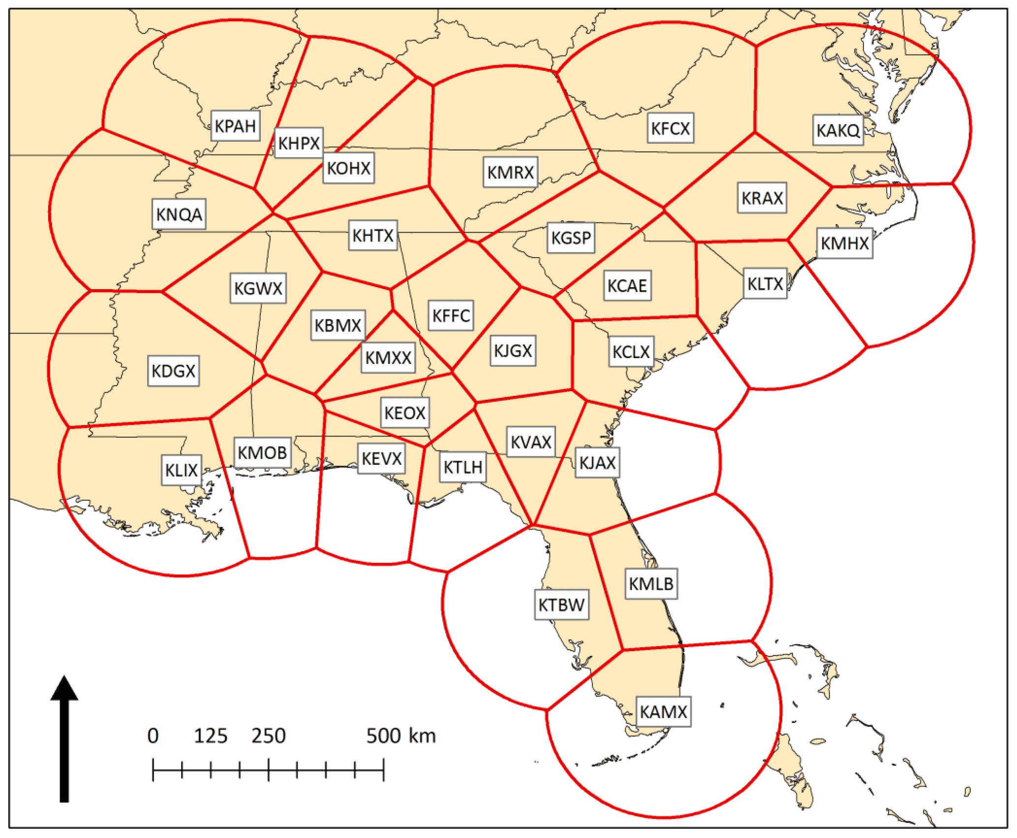
Table 1 Kinematic and thermodynamic parameters of 12:00 UTC composite soundings from Atlanta, GA, USA, for each radar-identified morphological type in Miller and Mote (2017). Morphological types classified as WFTs are bolded. All kinematic values are shown in m s⁻¹, whereas the units of the thermodynamic parameters are provided in the table. Explanations for the variable abbreviations can be found in Table 2 and Appendix A.

2 Data and methods

2.1 WFT selection and environmental characterization

This study uses the 15-year WFT dataset developed by Miller and Mote (2017) for the Southeastern US (Fig. 1). Their detection method first identifies thunderstorms as regions of spatiotemporally contiguous composite reflectivities meeting or exceeding 40 dBZ using connected neighborhoods labeling. Each thunderstorm is then assigned five morphological attributes describing its shape, duration, intensity, etc., and all thunderstorms are clustered into 10 morphologically similar groups using Ward's clustering (Ward, 1963). The composite convective environments associated with each morphological group were characterized using radiosonde observations from three launch sites in the Southeastern US. WFTs were designated as the subset of morphological groups with small, short-lived, diurnally driven thunderstorms that also formed in weak-shear, strong-instability composite environments. Table 1 provides the composite kinematic and thermodynamic environmental characteristics for the 10 morphological groups from Miller and Mote (2017). The WFTs are spatially referenced according to their first-detection location, the centroid of the composite reflectivities constituting the first appearance on radar. The storms were then paired with severe weather reports from the publication Storm Data, a storm event database maintained by the United States National Centers for Environmental Information, to differentiate benign WFTs from pulse thunderstorms. The entire 15-year dataset contains 885 496 WFTs including 5316 pulse thunderstorms.

Meanwhile, the thermodynamic and kinematic environment of each WFT was characterized using the 0 h Rapid Refresh (RAP) analysis. The RAP, implemented on 9 May 2012, is a 13 km non-hydrostatic weather model initialized hourly for the purpose of near-term mesoscale forecasting which is operated by the United States National Centers for Environmental Prediction. The RAP uses the National Oceanic and Atmospheric Administration (NOAA) Gridpoint Statistical Interpolation (GSI) system to assimilate radar reflectivity, lightning flashes (added in version 3), radiosonde observations, GOES cloud analysis, wind profiler data, surface station observations, etc. Lateral boundary conditions are provided by the Global Forecast System (GFS). Additional information regarding the RAP assimilation system and model physics can be found in Benjamin et al. (2016). The model has output available at 37 vertical levels spaced at 25 hPa intervals between 1000 and 100 hPa and 10 hPa intervals above 100 hPa. Several previous studies have relied upon the RAP's predecessor, the Rapid Update Cycle (RUC; Benjamin et al., 2004), to effectively characterize near-storm environments differentiating supercellular vs. non-supercellular and tornadic vs. non-tornadic thunderstorms (Thompson et al., 2007, 2014).

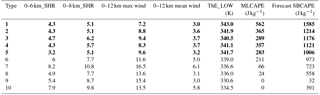
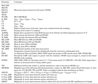
Table 2 List of the 31 convective parameters computed from the proxy soundings where CAPE, CIN, LCL, LFC, and EL and correspond to convective available potential energy, convective inhibition, lifted condensation level, level of free convection, and equilibrium level, respectively.

For the grid cell containing each WFT's first-detection location, a RAP proxy sounding was created using the SHARPpy software package (Blumberg et al., 2017). Thus, each proxy sounding represents the model-derived storm environment for a point no more than 13 km and 30 min distant from the WFT first-detection location. The proxy soundings were used to calculate 31 near-storm environmental variables and indices, a complete list of which is provided in Table 2 with more thorough descriptions in Appendix A. The 31 variables were largely selected by virtue of their accessibility in SHARPpy. Four warm seasons of the Miller and Mote (2017) dataset, containing 228 363 WFTs and 1481 pulse thunderstorms, overlapped with the RAP's operational archive period, allowing > 6 million near-storm parameters to contribute to the analysis.

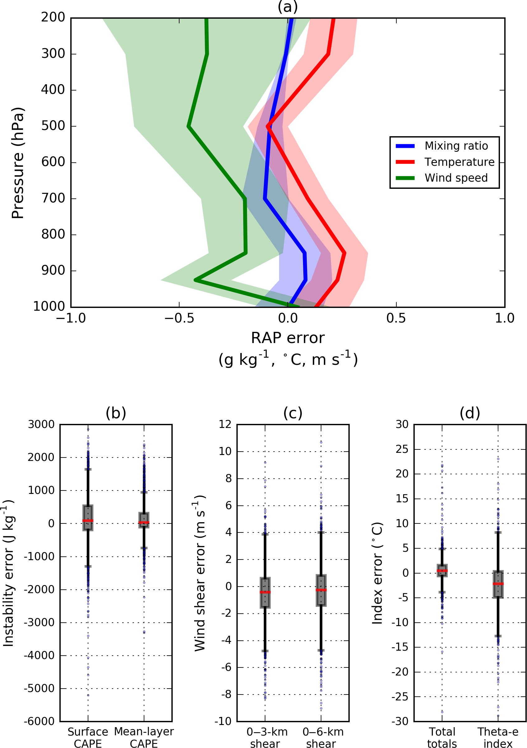
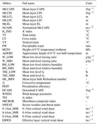
Figure 2 Vertical profiles of RAP output errors measured by co-located radiosonde observations (a). Errors were calculated at 1000, 925, 850, 700, 500, 300, and 200 hPa. The 95 % confidence interval for the mean error (solid lines) is shaded. Box plots of the resulting error for six derived quantities is shown in panels (b–d). The interquartile range (IQR), representing the middle 50 % of values, is depicted by the gray box. Values lying more than 1.5 × IQR from the median (red line) are marked with dots.

2.2 RAP error assessment

Thompson et al. (2003) demonstrated the suitability of the RUC, version 2 (RUC-2), to represent storm environments as evaluated using co-located radiosonde observations, and the Benjamin et al. (2016) RAP validation statistics show that the RAP is more accurate than its predecessor. Figure 2a shows the results of an error evaluation specific to the purposes of this study. Vertical error profiles were calculated for 3562 co-located RAP predictions and observed radiosonde profiles in the Southeastern US. The comparisons contain 00:00 and 12:00 UTC soundings during the warm season (May–September) between 2012 and 2015 at three launch sites along a north–south trajectory through the Miller and Mote (2017) domain: Nashville, TN, Peachtree City, GA, and Tampa, FL, corresponding to US radar identification codes KOHX, KFFC, and KTBW in Fig. 1. The synoptic station codes for these three sites are the same as their US radar identifications with the exception of Nashville, whose synoptic code is KBNA.

Similar to the Thompson RUC-2 analysis, the greatest, albeit small, temperature and moisture biases (mean errors) from the RAP reside near the surface and the upper atmosphere (Fig. 2a). Aided by the large sample of comparison soundings, the 95 % confidence intervals indicate that the true bias of the selected RAP output variables at these sites can be estimated with reasonable confidence. The 95 % mixing ratio confidence interval captures zero at all altitudes except 500 hPa, where the RAP predicted drier-than-observed values by 0.08 g kg⁻¹. Temperatures are warmer than observed throughout most of the troposphere with a maximum bias of 0.26 ^∘C at 850 hPa. In contrast, the RAP underestimated wind speeds on average throughout the depth of the troposphere. The largest bias, 0.46 m s⁻¹, was found at 925 hPa with similar errors above 500 hPa. The 95 % confidence interval for wind speed error is largest near the tropopause and demonstrates larger uncertainty than for temperature and mixing ratio. These results generally agree with the error statistics provided by Benjamin et al. (2016), and the reader should reference that paper for additional information, including validation statistics, about the RAP.

Table 3 RAP error statistics for surface-based CAPE (SBCAPE) and several of the variables listed in Table 2. The statistics are presented similarly to Thompson et al. (2003) by providing the mean RAP-derived value, the mean arithmetic error (bias), and the mean absolute error (MAE).

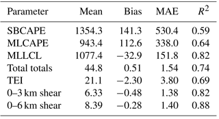
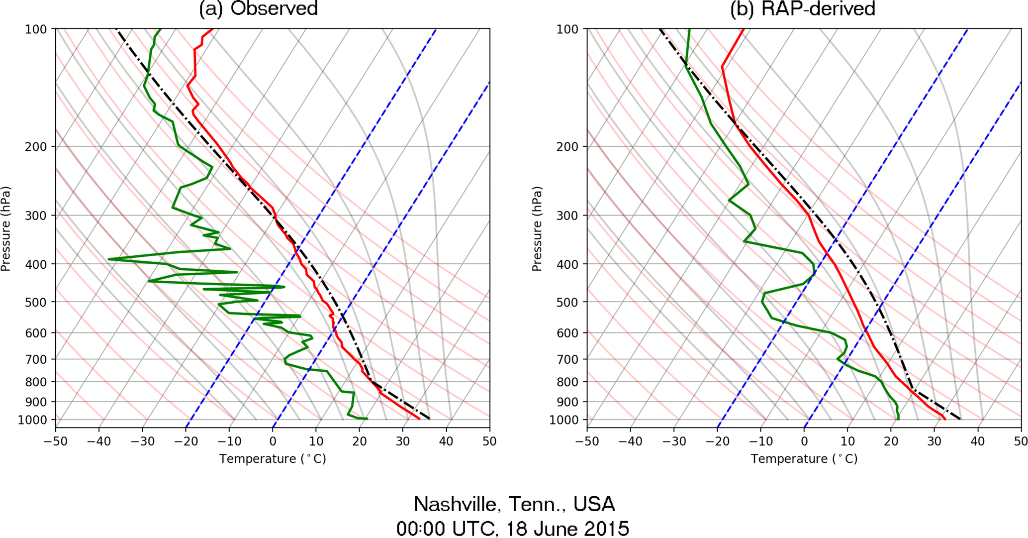
Figure 3 Comparison of observed (a) vs. RAP-derived (b) soundings for a case when the MLCAPE discrepancy exceeded 1000 J kg⁻¹ (observed: 1028 J kg⁻¹; RAP: 2051 J kg⁻¹). Minor mischaracterizations of low-level moisture contributed to a large response in MLCAPE during the vertical integration of the parcel trajectory.

Although the RAP appears to resolve temperature, mixing ratios, and wind speeds more accurately than the RUC-2, the transmission of these errors onto the derived convective parameters can be large. Table 3 expresses error measures for surface-based (SBCAPE) and mean-layer CAPE (MLCAPE), 0–3 km and 0–6 km wind shear, TTs, and TEI. Because the focus of this study is surface-based convection, only days when the observed surface-based CAPE was greater than zero were used to calculate the derived quantity error metrics. Similar to previous work (e.g., Lee, 2002), parameters calculated via the vertical integration of a parcel trajectory, such as CAPE, are sensitive to errors in low-level temperature and moisture. The RAP's low-level temperature and moisture biases influence the lifted condensation level (LCL) calculation (negative MLLCL bias; Table 3) yielding a premature transition to the pseudo-adiabatic lapse rate and an overestimate of parcel instability (positive SBCAPE and MLCAPE biases; Table 3)¹. Thompson et al. (2003) identified smaller CAPE errors generated by the RUC-2; however, the nature of the thermodynamic environments being examined is significantly different in this study. Similar to the RUC-2, the RAP is more adept at representing MLCAPE than SBCAPE with Fig. 2b and, consequently, the mean-layer parcel trajectory will be used for all parcel-related calculations.

In some cases, RAP proxy soundings may have been contaminated by premature convective overturning within the model. However, because the RAP assimilates radar reflectivity from the US (Benjamin et al., 2016), the 0 h RAP analysis fields should generally mirror the radar-observed areas of convection. Additionally, any such instances will be dampened by the methodological design decision to aggregate all proxy soundings on a daily level, as will be described in Sect. 2.3. The accuracy of the proxy soundings could be improved by employing a convection-permitting numerical model, such as the 3 km High-Resolution Rapid Refresh (HRRR). By explicitly modeling deep convection, the HRRR would limit convective contamination by more closely representing areas of thunderstorm activity. At the time of publication, the absence of a publicly accessible HRRR archive prevented its application in this research.

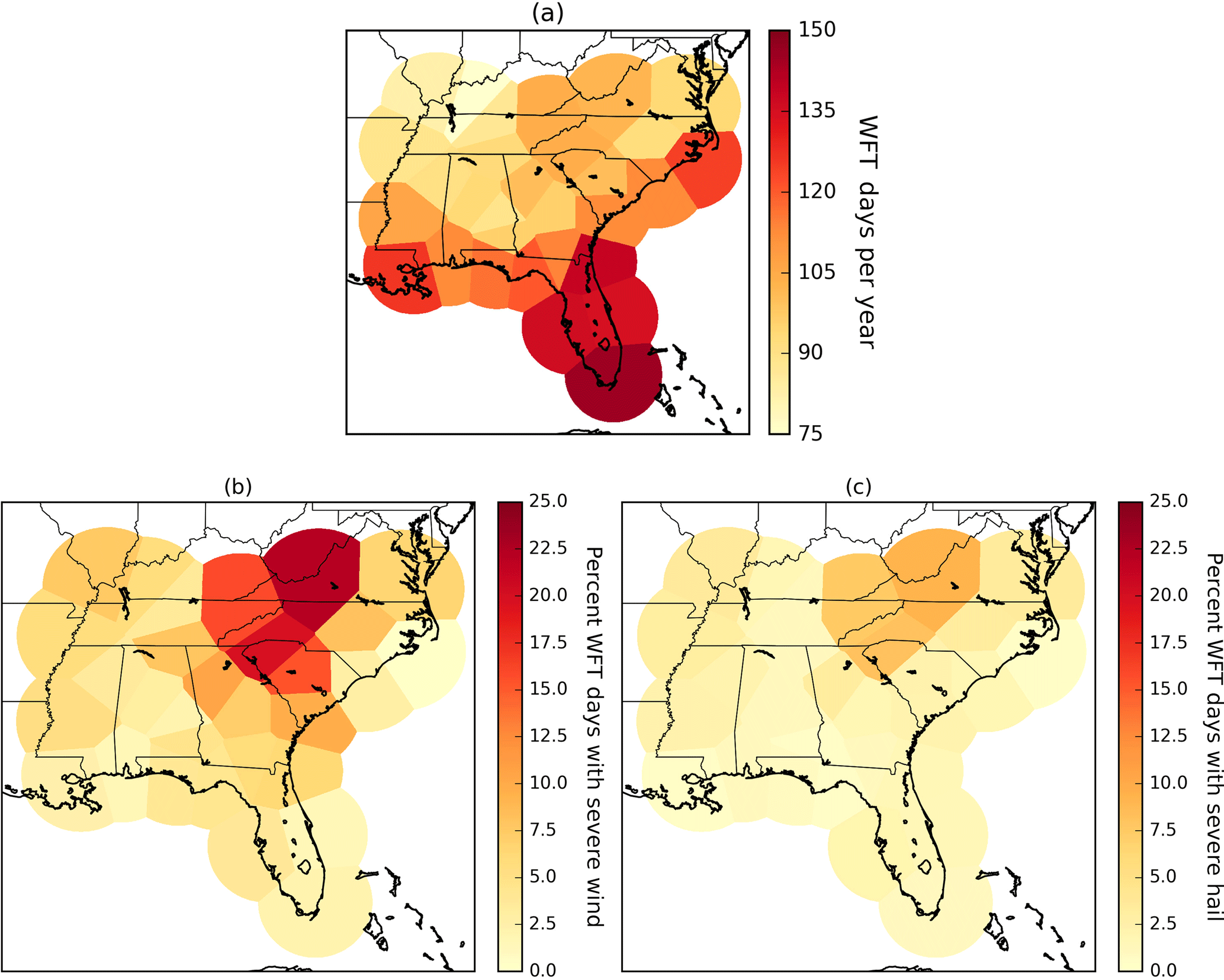
Figure 4 Average number of WFT days during the 4-year study period (a) compared to the proportion of WFT days affiliated with severe-wind (b) and severe-hail (c) events.

Table 4 WFT, SWS, and SHS day frequency by radar site.

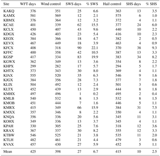
Figure 2b–d demonstrate that although large outliers certainly occur, the majority of RAP-derived thermodynamic and kinematic parameters are concentrated within a narrower range of error. Figure 3 provides an example skewT-logP diagram for a large MLCAPE error shown in Fig. 2d. Though the difference in this case exceeded 1000 J kg⁻¹, the discrepancy can largely be attributed to the RAP's minor mischaracterization of low-level moisture. Otherwise, the depiction of the vertical profile is reasonably accurate. The advantage of the RAP to represent the near-storm environment is underscored when compared to results from coarser-scale models. For instance, the coefficients of determination (R²) for RAP-derived SBCAPE and MLCAPE are appreciably larger than those calculated from the 32 km horizontal and 3 h temporal resolution North American Regional Reanalysis (NARR; Mesinger et al., 2006) in Gensini et al. (2014).

2.3 Assessing convective parameter skill

The quality of severe weather reports is a significant impediment to severe storm research (e.g., Miller et al., 2016; Weiss et al., 2002), particularly regarding the certainty with which non-severe storms can be declared non-severe. These storms may only appear benign because their associated severe weather was not reported. Consequently, the results of the proxy soundings are subdivided by nearest radar site (Fig. 1) and aggregated daily (12:00–12:00 UTC) by computing the mean parameter value associated with all WFTs forming within each polygon on a given day. Days containing at least one severe weather report are considered supportive of severe weather, whereas days with no severe weather reports will serve as the control. This approach is similar to the methods the Hurlbut and Cohen (2013) study of severe thunderstorm environments in the Northeastern US. Severe-wind-supporting (SWS) days and severe-hail-supporting (SHS) days are treated separately because their thermodynamic environments have been shown to contain unique elements related to downdraft and hailstone production (Johns and Doswell, 1992). Table 4 provides the specific subdivision details of the frequency of WFT days, SWS days, SHS days, and their respective control days. Figure 4 shows the annual average of WFT days for each radar site within the study area during the 2012–2015 warm seasons. As expected, WFT days are most frequent along coastlines and the Appalachian Mountains (Miller and Mote, 2017).

Given the low SNR in WFT environments, t tests are deceiving. Statistically significant differences in the mean values of parameters on severe vs. non-severe days are routinely reported, but the considerable overlap between the distributions (e.g., Craven and Brooks, 2004; Taszarek et al., 2017) can remove much practical value. This study explores the relationship between convective parameters and pulse thunderstorm environments by means of an odds ratio (OR; e.g., Fleiss et al., 2003). The OR is a common measure of conditional likelihood in human health and risk literature (e.g., Bland and Altman, 2000) with precedence in the atmospheric sciences (e.g., Black and Mote, 2015; Black et al., 2017). The OR looks past the descriptive statistics of the severe vs. non-severe distributions and more directly compares differences in where the data are concentrated within the distributions.

Equation (1) shows the standard definition of the OR, essentially the ratio of two ratios:

$$\begin{array}{}\text{(1)}& {\displaystyle }{\displaystyle }\text{OR}={\displaystyle \frac{A/C}{B/D}},\end{array}$$

where the numerator represents the ratio of events (A) to non-events (C) when a condition is met, whereas the denominator is the ratio of events (B) to non-events (D) when the same condition is not satisfied. In this context, “events” are SWS or SHS days whereas “non-events” would be the respective control days. Higher ORs indicate that events are more frequent (relative to non-events) when the condition is met, or conversely, that events are less frequent when the condition is not met. For this study, a condition might be a convective parameter exceeding a specified threshold. For instance, if the SWS OR equals 4 for the condition MLCAPE > 1000 J kg⁻¹, then the odds of an SWS day are 4× greater when MLCAPE is greater than 1000 J kg⁻¹ than when it is less than 1000 J kg⁻¹.

We employ a modified form of the OR in which both the numerator and denominator are standardized by the climatological ratio of events to non-events (Eq. 2), allowing the components of the OR to be separated and interpreted independently by comparison to climatology.

$$\begin{array}{}\text{(2)}& {\displaystyle }{\displaystyle }\text{OR}={\displaystyle \frac{\frac{A/C}{(A+B)/(C+D)}}{\frac{B/D}{(A+B)/(C+D)}}}\end{array}$$

The modification does not change the value of the quotient OR, but it does improve the interpretability of the numerator and denominator. When the numerator or denominator is near 0 (1), then the odds of SWS or SHS days are much lower than (nearly equal to) climatology. The climatological odds ratio was 0.069 for SWS days and 0.025 for SHS days. A 95 % confidence interval for the OR was calculated using the four-step method presented in Black et al. (2017).

Table 5 Summary of convective parameters on SWS days. The “sites” column indicates the number of spatial subdivisions within which the difference between the SWS mean and the control mean was accompanied by p < 0.10; the “percent change” column shows the relative increase or decrease of the mean on SWS days.

3 Results

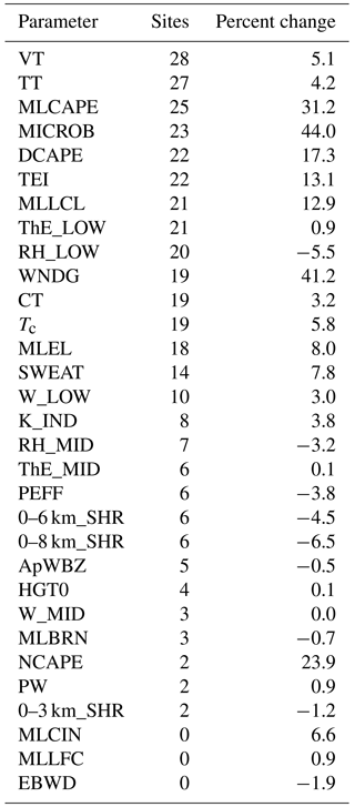
3.1 Convective environments of pulse thunderstorm wind events

During the 4-year study period, pulse thunderstorm wind events were documented somewhere in the study area on 49 % of WFT days, although the average frequency within any single subdivision was 6.7 % (Table 4). Table 5 shows the 31 convective parameters analyzed from the proxy soundings as well as the number of subdivisions for which each parameter is a statistically significant differentiator of SWS days. A significance threshold of p < 0.10 guided the selection of potentially useful parameters which would be examined in more detail. Nine of the 31 variables are statistically significant across at least two-thirds of the study area: VT, TT, MLCAPE, MLLCL, MICROB, DCAPE, TEI, RH_LOW, and ThE_LOW.

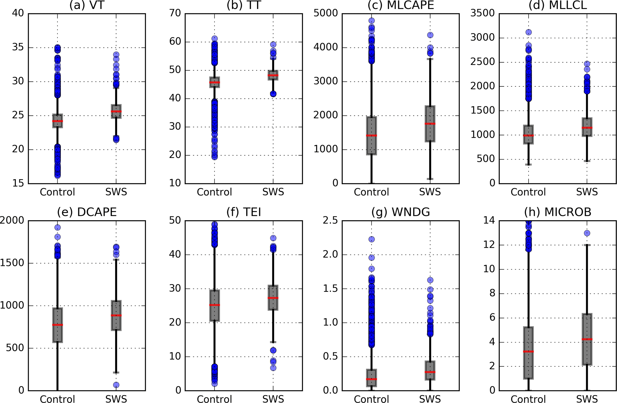
Figure 5 Box plots of selected convective parameters that demonstrated skill in differentiating between the control days and SWS days.

Figure 5a–h depict the distributions for several parameters from Table 5 for control vs. SWS days. These eight parameters are significant across much of the domain (VT and TT), demonstrate larger relative changes on SWS days (MLCAPE and MLLCL), and/or are traditional operational severe-wind forecasting tools (DCAPE, TEI, WNDG, MICROB). However, as the distributions clearly illustrate, any difference in the mean values between the control days and SWS days is small compared to the spread about their means. This results in the characteristically low SNR described in the Sect. 1. Any attempt to establish a forecasting value indicative of pulse-wind potential will yield many missed events occurring beneath the threshold and/or false alarms associated with control days above it.

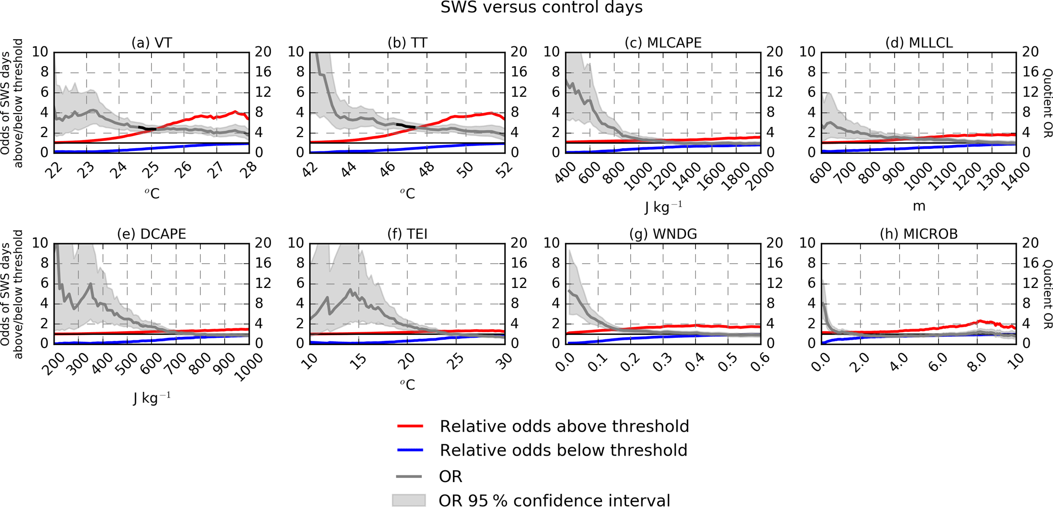
Figure 6 ORs for the same eight convective parameters shown in Fig. 5. Whenever the OR, defined by Eq. (2), results from a numerator (red) ≥ 2 and a denominator (blue) ≤ 0.5, then the OR is drawn in black. The left y axis expresses values corresponding to the OR's numerator and denominator (red and blue lines), and the right y axis corresponds to the OR value (gray line). At very low and very high threshold values, the variance of the OR may be undefined, and the 95 % OR confidence interval cannot be computed.

Thus, Fig. 6 employs the OR to characterize the relative skill that some knowledge of the convective environment can contribute to a severe vs. non-severe designation. For each variable in Fig. 5, a progressively larger value is selected, and the OR is calculated at each step. Figure 6 displays the OR as well as both the numerator and denominator terms for each iteration. High ORs can often result when a near-zero number of severe events exist below the threshold inflating the OR calculation. In these situations, the OR is indicating that severe weather is very unlikely rather than that the severe weather risk is enhanced. These results are not particularly useful because forecasters would not have needed a decision-support tool in these environments in the first place. Ideally, large ORs will result when the numerator indicates an appreciable increase against the climatology while the denominator simultaneously indicates an appreciable decrease below climatology. Further, these ORs would ideally occur in a range where the severe weather risk may be uncertain. In Fig. 6, the OR is shown in a gray line, but the line is drawn in black whenever the OR results from a numerator ≥ 2 and a denominator ≤ 0.5. ORs resulting from this combination indicate that the threshold yields a simultaneous 2-fold increase (decrease) in the odds of SWS days above (below) the specified value. These ORs will be hereon referenced as “2-fold” ORs and represent a goal scenario.

Figures 6a–h show ORs for the same eight parameters in Fig. 5. Of all eight parameters, only VT and TT achieve 2-fold ORs for any range of thresholds, as indicated by the black segments in Fig. 6a and b. The maximum 2-fold OR for VT is 5.16 at 24.6 ^∘C, meaning that the odds of an SWS day are 5.16× greater when this threshold is met. TT offers slightly more skill with a maximum 2-fold OR of 5.70 at 46.5 ^∘C. As described in Appendix A, VTs and TT s are relatively primitive indices. VT is purely a temperature lapse rate whereas TT is predominantly a measure of lapse rate with an additional dew point term included. Meanwhile, MLCAPE and MLLCL demonstrate consistently lower ORs between 2 and 4. The four wind-specific variables in Fig. 6e–h are relatively poor differentiators of SWS days in the WFT regime. The maximum OR achieved by any of these parameters is approximately 10 driven by very low values of DCAPE with corresponding wide confidence intervals.

Though ORs are greater at lower VT and TT thresholds, these values are also somewhat common. Placing the aforementioned values (24.6 and 46.5 ^∘C, respectively) in the context of the 12 759 WFT environments included in this study, they represent the 58.8th and 58.9th percentiles of their distributions. Alternatively, the maximum VT threshold that yields a 2-fold OR is 25.1 ^∘C, which corresponds to the 70.9th percentile of all VTs in the dataset; however, the OR for this value is smaller, 4.77. This result illustrates the trade-off involved by seeking climatologically exceptional values to serve as guidance. As greater values are selected as the threshold, meteorologists can focus on a fewer number of days. However, the OR decreases as more severe weather events occur in environments not satisfying the threshold. As for TT, the maximum 2-fold OR value is 47.3 ^∘C, corresponding to the 70.6th percentile, but demonstrates an OR of 5.16. This means that when TT meets or exceeds 47.3 ^∘C, the odds of a pulse thunderstorm severe-wind event are 5.16× greater than when it does not.

Table 6 Same as Table 5, except for SHS days.

3.2 Convective environments of pulse thunderstorm hail events

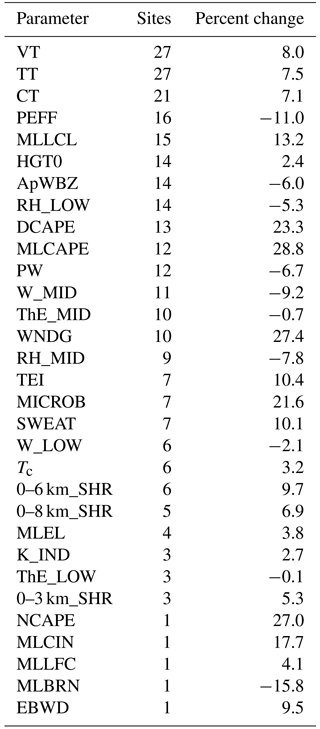
Table 6 replicates Table 5 except for SHS days. Many of the same parameters that are statistically significant differentiators of SWS days also rank high for SHS days. However, fewer parameters in Table 6 are statistically significant over two-thirds of the domain. Whereas 10 parameters in Table 5 showed spatially expansive statistical skill on SWS days, only three quantities do so on SHS days. We attribute this result to the pattern in Table 4 and Fig. 4b and c whereby there are fewer SHS days than SWS days, which increases uncertainty related to the statistical tests and makes it harder to confidently detect differences.

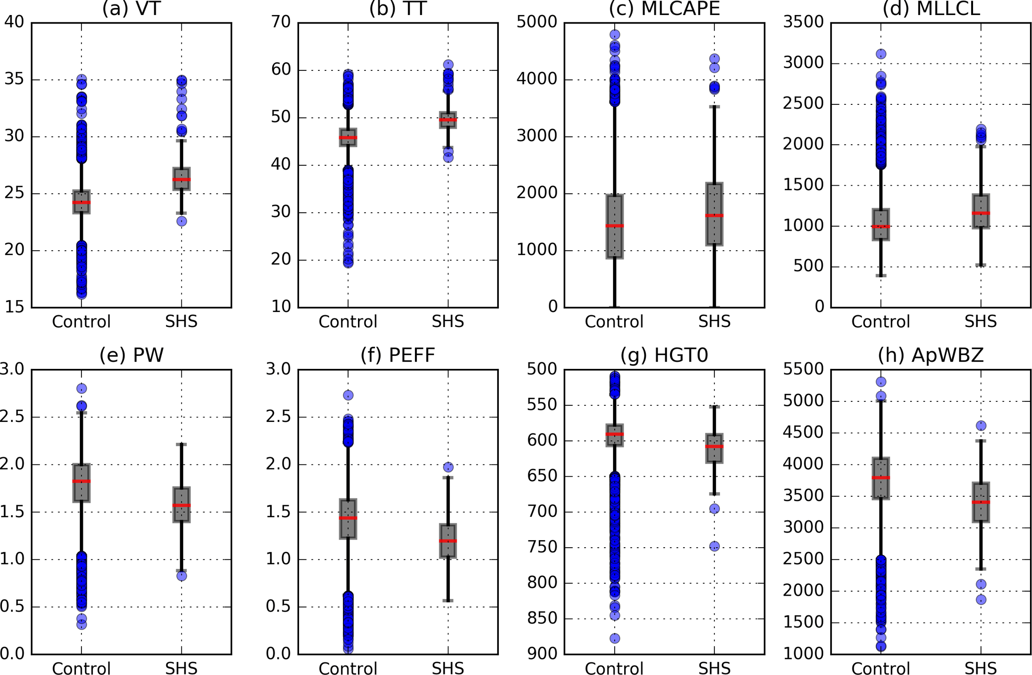
Figure 7 Same as Fig. 5 except for SHS days. Panels (a–d) replicate the same variables shown in Fig. 5, whereas (e–h) are replaced with four SHS-specific parameters from Table 6.

Nonetheless, VT and TT are once again skillful differentiators and are now joined by their related parameter CT. Additionally, several new convective variables demonstrate statistical significance across roughly half of the domain on SHS days that demonstrated little skill on SWS days: PW, PEFF, HGT0, and ApWBZ. For comparison, Fig. 7a–d duplicate Fig. 5a–d, now comparing distributions between the control and SHS days, while Fig. 7e–h display box plots for the SHS-specific convective parameters listed above. The distributions for MLCAPE and MLLCL are similar; however, there is a larger separation between control and SHS days for VT and TT than was apparent on SWS days. This observation is corroborated by the relative changes in VT and TT on SHS days that are several percentage points larger than for SWS days (Table 6). PW, PEFF, HGT0, and ApWBZ demonstrate smaller differences.

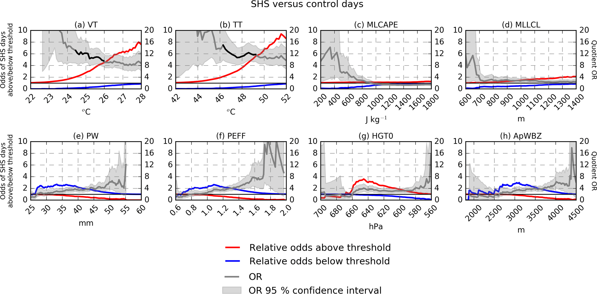
Figure 8 Same as Fig. 6 except for SHS days. Panels (a–d) replicate the same variables shown in Fig. 6, whereas (e–h) are replaced with four SHS-specific parameters from Table 6. At very low and very high threshold values, the variance of the OR may be undefined, and the 95 % OR confidence interval cannot be computed.

Figure 8 replicates Fig. 6 except by representing SHS days and substituting the four wind-specific parameters (DCAPE, TEI, WNDG, MICROB) with the four hail parameters listed above (PW, PEFF, HGT0, ApWBZ). The ORs for VT and TT are large, greater than 10, throughout the entire range of thresholds tested, and contain larger swathes of 2-fold ORs. The maximum 2-fold OR for VT is 13.1 at 24.4 ^∘C, and the maximum VT threshold that achieves a 2-fold OR is 26.0 ^∘C with an OR of 9.61. These values relate to the 53.4th and 86.0th percentiles of the VT distribution. As for TT, the maximum 2-fold OR is 14.98 at 46.3 ^∘C, and the maximum 2-fold-OR threshold is 49.2 ^∘C with an OR of 11.79. These two TT cutoffs translate to the 55.7th and 88.4th percentiles. Similar to SWS days, MLCAPE and MLLCL show little skill with ORs generally between 1 and 2. PW, PEFF, HGT0, and ApWBZ perform more capably than MLCAPE and MLLCL; however, they do not produce any 2-fold ORs. Values for these metrics are generally around 4 with several instances of higher ORs driven by a small denominator with wide 95 % confidence intervals.

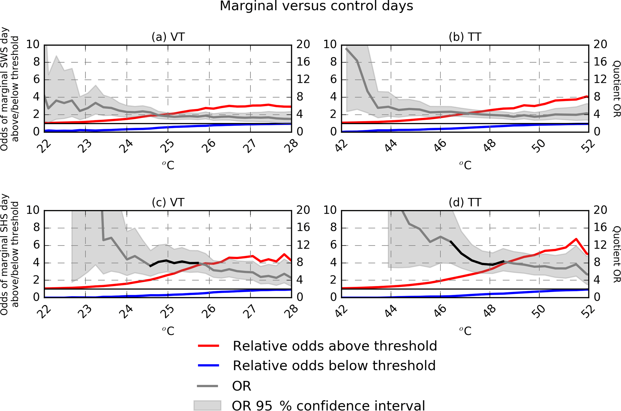
Figure 9 Same as Fig. 6a and b (a, b) and Fig. 8a and b (c, d) except that only marginal SWS and SHS days are used to calculate the OR. At very low and very high threshold values, the variance of the OR may be undefined, and the 95 % OR confidence interval cannot be computed.

3.3 Separating marginal pulse thunderstorm days

Because the severe weather generated by pulse thunderstorms is often near the lower limit used to define severe weather in the United States, some pulse thunderstorm environments may closely resemble non-severe regimes. Consequently, the influence of these “marginal” pulse thunderstorm days on the OR analysis is further scrutinized. For this purpose, “marginal” SWS and SHS days are defined as those on which only one severe wind or hail report was received. Marginal days constitute 48.7 % of the SWS days and 57.7 % of the SHS days in Table 4. Figure 9 replicates the OR analysis for VT and TT, the two most promising environmental parameters from Sects. 3.1 and 3.2, but with only marginal SWS and SHS days being considered. Comparing Figs. 6a and b and 8a and b to Fig. 9, marginal SWS and SHS days resemble the OR patterns of the broader set of SWS (Fig. 6a and b) and SHS (Fig. 8a and b) days. Though the ORs for the marginal subset are slightly smaller than for the broader group, they bear similar OR patterns as the thresholds are increased. Overall, marginal SWS and SHS days are generally characterized by similar VT and TT values as when all SWS and SHS days were aggregated. Corroborating this finding, an OR analysis comparing marginal SWS and SHS days to those with > 1 severe event (not shown) revealed that ORs generally remained near 1 regardless of the VT or TT threshold selected. Thus, although marginal pulse thunderstorm days are by no means easily distinguishable from non-severe WFT days, they do not appear to be particularly more challenging to differentiate than active pulse thunderstorm days.

4 Discussion

The relative changes in the convective variables in Table 5 on SWS days vs. control days correspond well to previous microburst research. Compared to the non-severe control days, SWS days are characterized by a drier near-surface layer (i.e., lower RH, higher LCLs). Simultaneously, steep mid-level lapse rates (i.e., larger VT and TT) aid an increase in CAPE which supports stronger updrafts. As the strong updraft transitions to a downdraft-dominant storm, the drier surface layer supports evaporative cooling, downdraft acceleration, and severe outflow winds. This same conceptual model has been promoted by previous severe convective wind research (e.g., Atkins and Wakimoto, 1991; Kingsmill and Wakimoto, 1991; Wolfson, 1988).

The results of SHS days also support previous findings (Johns and Doswell, 1992; Moore and Pino, 1990; Púčik et al., 2015). The distributions in Fig. 7 (and relative changes in Table 6) indicate that SHS days are characterized by relative decreases in PW, a lower freezing level, a lower wet-bulb freezing level, and dry near-surface air. Smaller PWs result in less waterloading and greater parcel buoyancy (larger VT, TT, and MLCAPE), which maximizes updraft strength. Meanwhile, lower freezing levels and a dry layer between 1000 and 850 hPa support evaporative cooling which can together yield a lower wet-bulb zero height and limit hail stone melting during its descent to the surface. Interestingly, these two concepts are both represented in the PEFF calculation (Appendix A), which was not developed as a hail indicator. PEFF as defined by Noel and Dobur (2002) equals the product of PW and the mean 1000–700 hPa RH. As both values decrease, PEFF becomes smaller and hail is more likely for the reasons stated above.

The poor performance of MLLCLs and MLCAPEs in differentiating SWS and SHS days from their controls is surprising given their prominence in severe storm forecasting. One possibility is that the daily aggregation of MLCAPEs may have smoothed out locally higher values near the WFTs that were responsible for severe weather production. Alternatively, VT and TT were among the strongest indicators of both SWS and SHS days. Recalling from Sect. 2.2, VT and TT are also very well represented by the RAP. TTs were replicated by the model with a < 1 ^∘C bias and a MAE representing only 3 % of the average value (Table 3). Additionally, mid-level temperatures, from which VT is computed, also compared very well to the observed soundings (Fig. 2a). The strong performance of VT and TT compared to other more heavily moisture-weighted metrics may be due to their more accurate representation in the proxy soundings.

Regardless, because the severe weather SNR is already low in WFT environments, any systematic error introduced by the data source (in this case the RAP) may significantly dampen, or even remove, whatever environmental differences exist. As Sect. 2.2 indicated and previous work has also concluded, low-level moisture biases can impede the accurate calculation of convective parameters relying on those terms (e.g., Gensini et al., 2014; Thompson et al., 2003). In this study, MLCAPE, MLLCL, PW, PEFF, and others were vulnerable to such errors. The poorer performance of these variables' ORs (relative to the lapse-rate-based parameters) and the sensitivity of PW, PEFF, and ApWBZ to simulated RAP errors suggests that model inaccuracies may be obscuring their potential skill to detect weakly forced severe weather environments. The perception of the WFT environment as a difficult-to-forecast regime may partly be driven by model inconsistency exacerbating an already small SNR.

Another confounding factor is the quality of the Storm Data severe weather reports. Section 3.3 discussed that marginal SWS and SHS days are more similar to days with > 1 report than days with no reports. Thus, the basis for the similarity may be that severe weather was simply under-reported on “marginal” days. Extending this logic, the pulse regime's low SNR may also be partially attributed to under-reporting of severe weather on “non-severe” days. Given that the severe weather generated by pulse convection is often short-lived, isolated, and narrowly exceeds severe criteria, the notion that some pulse-related severe weather events go undetected is likely. If some “non-severe” days existing above the tested parameter thresholds in Figs. 6 and 8 did in fact host severe weather, then the ORs would have been larger than those found in Sects. 3.1 and 3.2.

5 Conclusions

Hazardous weather within WFT environments is characterized by a lower SNR than other severe thunderstorm regimes. Though past research has developed promising tools for forecasting pulse thunderstorm environments, their relatively small samples sizes may have understated the SNR and, by corollary, overstated the reliability of their tools. With recent research suggesting that the performance of new severe weather forecasting tools is closely tied to the proportion of non-severe thunderstorms in the sample (Murphy, 2017), this study sought to test the relative skill of 31 convective forecasting parameters using realistic proportions of severe and non-severe WFT environments (severe: 7.9 %; non-severe: 92.1 %). Future research may consider broadening the methods of Murphy (2017) to standardize the skill values across previous studies of severe convective environments.

Only 13 (5) of the 31 convective parameters tested were statistically significant (p < 0.10) differentiators of SWS (SHS) days across at least half of the domain. Though the distinctive variables for SWS and SHS days were consistent with previous theories of severe microburst and hail formation, considerable overlap between the distribution of values on severe and non-severe days is problematic. Similarities between the SWS, SHS, and their corresponding control distributions inhibit consistent identification of pulse thunderstorm potential based on the value of any individual parameter. Nonetheless, VT and TT did perform more skillfully than the others. When VTs exceed values between 24.6 and 25.1 ^∘C or TTs between 46.5 and 47.3 ^∘C, the relative odds of a wind event increases roughly 5×. Meanwhile, the odds of a hail event become roughly 10× greater when VTs exceed values between 24.4 and 26.0 ^∘C or TTs between 46.3 and 49.2 ^∘C.

The noteworthy performance of VT and TT, two quantities calculated from the more reliable RAP output fields, is unlikely a coincidence. Our findings suggest that the already weak severe weather SNR in WFT environments is exacerbated by model limitations in the low-level moisture and temperature fields. Meteorologists may perhaps alleviate the challenges of the WFT environment by examining convective parameters that are well-represented by models, such as VT, TT, and other measures of lapse rate. Future research might seek to track the transmission of the model errors through calculation of forecast skill statistics and more concretely ascertain the contribution of model error to the SNR.

Appendix A:  

Table A1 Additional detail describing the convective parameters in Table 2.