Spatial structures of emerging hot and dry compound events over Europe from 1950 to 2023

Compound events (CE), characterized by the combination of climate phenomena that are not necessarily extreme individually, can result in severe impacts when they occur concurrently or sequentially. Understanding past and potential future changes in their occurrence is thus crucial. The present study investigates historical changes in the probability of hot and dry compound events over Europe and North Africa, using ERA5 reanalyses spanning the 1950–2023 period. Two key questions are addressed: (1) Where and when did the probability of these events emerge from natural variability, and what is the spatial extent of this emergence? This is explored through the analysis of “time” and “periods” of emergence, noted ToE and PoE, defined as the year from which and the moments during which changes in compound event probabilities exceed natural variability. The new concept of PoE allows for more in-depth signal analysis. (2) What drives the emergence? More specifically, what are the relative contributions of changes in marginal distributions versus in the dependence structure to the change of compound events probability? The signal is modelled with bivariate copula, allowing for the decomposition of these contributions. A focus on the dependence component is explored to quantify its effect on the signal's emergence. The results reveal clear spatial patterns in terms of emergence and contributions. Five areas are studied in greater depth, selected for their contrasted signal behaviors. In some regions, the frequency of hot and dry events increased, mainly due to a change in the marginals. However, other regions see a decrease of CE probabilities, mainly driven by a change in the drought index. Although the dependence component is rarely the main contributor to PoE, it remains necessary to detect signal's emergence. Without considering the dependence component, the date of ToE and the duration of PoE can be overestimated as well as underestimated (even more than 20 years) depending on the area. These findings provide new insights into the drivers of CE probability changes and open avenues for advancing attribution studies, ultimately improving assessments of risks associated with past and future climate change.

1 Introduction

For several years, Europe has faced severe hot and dry events, corresponding to a combination of drought and heatwave. This climate phenomenon, such as during summer 2018, has significantly affected various sectors of society (Rousi et al., 2023). It has impacted biodiversity with an increased fire risk during this period (San-Miguel-Ayanz et al., 2019), agriculture with yields falling by up to 50 % (Toreti et al., 2019), and human health with an increased number of deaths (Pascal et al., 2021). In 2022, the continent experienced another unprecedented hot and dry event, particularly severe with respect to previous ones (Tripathy and Mishra, 2023). This type of event is categorized as a compound event (CE), “a combination of multiple drivers and/or hazards that contribute to societal or environmental risk” (Zscheischler et al., 2020). Taken individually, the univariate hazards (e.g., heatwave and drought) are not necessarily extreme but their concurrent or sequential occurrences can cause severe impacts and damages, higher than if they occur separately. The non linear relationship between the hydro-climatic variables (e.g., extreme temperature and lack of precipitation) plays a key role for understanding CE (Hao and Singh, 2016). In Europe, if hot and dry events are considered independent, the CE occurrence can be underestimated by a factor of up to 8 over the continent when both variables exceed their 95th percentiles of the reference period (1950–1979) (e.g., Manning et al., 2019).

In Europe, an increase in the frequency and intensity of hot and dry events has been observed since 1950 (Manning et al., 2019) and this trend is expected to continue in the future (Ridder et al., 2022). This is also the case for other CEs, such as compound floodings, due to co-occurring extreme wind and precipitation, that are also becoming more frequent along the European coasts (Bevacqua et al., 2019). The impact of an absolute change depends on the range of natural variability, whether the environment is accustomed to such changes. Ecosystems and species adapted to large natural variability, may be less affected by climate change (Williams et al., 2007). Conversely, species with limited adaptability, such as certain tropical plants, insects, and reptiles, are more vulnerable to warming and climate changes (Deutsch et al., 2008). It is thus important to quantify this CE increase relative to natural variability. To do so, the notion of “emergence” is usually defined as the ratio between the estimated climate change signal (S) and the noise (N) associated to natural variability. A “Time of Emergence” (ToE) is then identified as the first year for which the ratio permanently exceeds a threshold, 1, 2 or 3, corresponding to an “unsusual”, “unfamiliar” or “unknown” emergence, respectively (Frame et al., 2017). Another popular approach consists in detecting when a distribution is statistically different from the reference period, based on a statistical test between distributions, such as the Kolmogorov–Smirnov test (e.g., Mahlstein et al., 2012; King et al., 2015; Gaetani et al., 2020) or based on distances between distributions, such as the Hellinger distance (Pohl et al., 2020).

Emergence of multivariate events remains largely underexplored. The great majority of studies analyses the emergence at a global scale and for univariate variables: mainly temperature (e.g., Diffenbaugh and Scherer, 2011; Mahlstein et al., 2011; Hawkins and Sutton, 2012) and precipitation (e.g., Giorgi and Bi, 2009; Fischer and Knutti, 2014; Murphy et al., 2023), but also drought index (Ossó et al., 2022), fire weather index (e.g., Abatzoglou et al., 2019), sea level (e.g., Lyu et al., 2014) and biogeochemical cycle (Keller et al., 2014). As compound events contribute to the most damaging impacts (Zscheischler et al., 2020), the question of multivariate emergence has recently arisen. The understanding of past and future changes of compound events occurrence is of great importance for adaptation planning. The goal is now to detect when a multivariate distribution is statistically different from a baseline period. Williams et al. (2007) used the standardized Euclidean distance to quantify the differences between two climates in the 20th and 21st centuries. Mahony et al. (2017) adapted this metric to take the covariance between variables into account with the Mahalanobis distance. The latter, transformed into percentiles of the chi distributions, is called “sigma dissimilarity” and has been used to identify multivariate climate departures (e.g., Abatzoglou et al., 2020; Mahony and Cannon, 2018). However the dependence between the variables is assumed to be Gaussian, i.e., fully characterized by a covariance matrix. This implies that only linear relationships are captured, and any non-linear or asymmetric dependence – particularly in the extremes – is ignored. This approach is not well suited for analyzing compound extremes, where the focus lies on understanding how variables co-occur specifically in the tails of the distributions (e.g., Zscheischler et al., 2020; Tootoonchi et al., 2022). Capturing such behavior requires more flexible dependence structures beyond the Gaussian framework (Hao and Singh, 2016). That is why, François and Vrac (2023) defined a time of emergence (ToE) applicable to multivariate events, as the year from which the compound event probability (the signal) is always out of the natural variability. In this method, the signal is quantified with bivariate copula, which allows a modeling of a not Gaussian dependence.

Time of emergence provides limited information. Climate system is highly nonlinear and non-monotonic, detecting the emergence of a signal using ToE can be limited depending on the climate signal under study. ToE detects a significant change only if the latter is permanent until the last year of the studied period (Mahlstein et al., 2012). If the variable remains within the bounds of natural variability, no information is given. As ToE detection only needs the first and the last values of a time series, we do not know what happened in between. Two signals that do not emerge, i.e., finally come back to the range of natural variability may have evolved differently, and even oppositely. In the same way, two signals that emerge simultaneously may have behaved distinctly. The signal could vary in the opposite direction to the final ToE. For example, the signal could significantly decrease below the lower bound of natural variability before sharply increase above the upper bound. Abrupt changes in probability out of natural variability could lead to severe damages if society or human activities are not adapted to such events. Bevacqua et al. (2024b) found that a year above 1.5 °C could very likely announce the beginning of a 20-year period with an average warming above the same threshold. In the same way, variations of probabilities near the upper bound of the natural variability could also help to anticipate ToE. Although not represented through the ToE metric, such variations, called “Periods of Emergence” (PoE) could be linked to the expected impacts. This new metric can be highly beneficial for adaptation planning in a lot of fields. For example, the agricultural sector may question whether they are entering a new phase of unusual compound events and seek to understand if similar situations occurred in the past to better anticipate impacts on water availability and decide which crops to cultivate. The present study takes advantage of ToE definition from François and Vrac (2023) paper and extends it to PoE concept.

From a statistical point of view, the probability of a bivariate compound event relies on three components: the two marginal (i.e., univariate) distributions and the dependence structure coupling them. Consequently, significant probability changes with respect to a reference period can be due to either an evolution of the univariate distributions or a change in their inter-relationship. Studies showed that the change of hot and dry occurrences are mostly due to a change in temperature (Ionita and Nagavciuc, 2021) or a shift in precipitation deficit (Manning et al., 2018). On the other side, the strength of the dependence is crucial for CE analysis (François and Vrac, 2023). If the variables are (falsely) considered independent, the CE occurrence can be strongly underestimated (e.g., Zscheischler and Seneviratne, 2017). However the dependence change is little studied (e.g., Wang et al., 2021). In this study we want to analyse all three statistical components forming the CEs in order to quantify which one contributes the most to the emergence. A method for disentangling the contributions of the marginals and those of dependence to the total change in CE probability will then be proposed, relying on copula theory that allows to model dependencies in CE variables (e.g., Bevacqua et al., 2019; Manning et al., 2019; Li et al., 2022).

Thanks to the introduced notions (times and period of emergence, copula theory and contribution metrics), the present study aims to develop a method for detecting and characterizing changes in probabilities of bivariate CEs. The proposed approach will be applied to hot and dry compounds over Europe from 1950 to 2023, based on reanalysis dataset. The main goals are to investigate if we can already see changes in hot and dry CE probabilities within the last few decades; where and when the signal emerged; if spatial patterns are visible; and which statistical component of the CE contributes the most to a change in CE probability.

The rest of this article is organized as follows. The data used and the CE emergence method will first be presented in Sect. 2. The computation of the different contributions and the influence of the change in dependence on the emergence will then be given in Sect. 3. Finally, the results for hot and dry events over Europe will be presented in Sect. 4 before concluding and providing the main conclusions and some perspectives in Sect. 5.

2 Data and Method

2.1 Data

The present study uses ERA5 daily reanalysis (Hersbach et al., 2020), the fifth generation from the European Center for Medium-Range Weather Forecasts (ECMWF), in Europe and North Africa. The data are available on a regular grid at a 0.25° × 0.25° spatial resolution (22 394 grid points), between 1950 and 2023.

Hot and dry events are usually studied during summer (June–July–August), the probability of occurrence is higher and the heat stress deadlier during this season (Shan et al., 2024). Mid-latitudes experience greater climate variability in winter, which reduces the warming-to-variability signals in most regions, despite the overall increase in warming (Mahlstein et al., 2011). Thus temperature emerges sooner during summer (Hawkins and Sutton, 2012). The most commonly used variables for analysing this compound event are temperature and precipitation (e.g., Zscheischler and Seneviratne, 2017; Singh et al., 2021; Bevacqua et al., 2022). Lack of rainfall usually refers to meteorological drought (Wilhite and Glantz, 1985). Three other types of drought have major impacts on society: hydrological drought, related to low surface and subsurface water resources; agricultural drought, associated with very poor soil moisture; and socio-economic drought characterized by an imbalance between water demand and need (Mishra and Singh, 2010). This classification implies the use of several drought indices, such as: the Palmer Drought Severity Index, PDSI (Palmer, 1965), the Standardised Precipitation Index, SPI (McKee et al., 1993) and the Standardised Precipitation-Evapotranspiration Index, SPEI (Vicente-Serrano et al., 2010). The latter is based on the difference between precipitation and evapotranspiration, reflecting the water balance. The SPEI indicator, considered to be one of the best for drought monitoring (e.g., Ionita and Nagavciuc, 2021; Blauhut et al., 2016), is used for the present study as it combines the advantages of SPI, with its variety of timescales, and those of PDSI with the consideration of temperature evolution. Depending on the chosen accumulation period, it can capture the different types of drought (Ionita and Nagavciuc, 2021). Then the analysis is performed at a monthly time scale to match the temporal resolution of the SPEI.

Hence, in the present study, hot and dry compound events are investigated through the two following variables at grid point scale over the summer (June, July, August) months: monthly maximum of daily maximum temperature, denoted T_max, on the one hand, and the monthly value of the 6-month standardised precipitation-evapotranspiration index (SPEI6) on the other hand. The number 6 refers to the number of previous months taken into account in the calculation of SPEI: here, 6 is chosen to include some winter and/or early spring months in the drought index calculation since a lack of precipitation in the preceding months promotes summer heatwaves (e.g., Quesada et al., 2012; Russo et al., 2019). For modelling reasons, in the following, the variable S = −SPEI6 will be used instead of SPEI6. A severe drought (indicated by negative SPEI6 values) will be characterized by a high positive value of S and wet conditions will be described by low (negative) S values.

2.2 Signal definition

The signal considered in this study is the CE probability quantified with bivariate copula. The copula function is a statistical tool that allows to model the dependence between variables, independently of their marginal distributions. It has been introduced by Sklar (1959), who established that any multivariate joint distribution can be written as a copula function applied to the marginal distributions. This approach has been applied to various hydroclimatological cases since the early 2000s (e.g., Favre et al., 2004; Salvadori and De Michele, 2004). Let us consider two random variables X and Y, with their cumulative distribution functions (CDF) F_X and F_Y. The joint CDF H can be expressed as follows:

$$\begin{array}{}\text{(1)}& \begin{array}{rl}H(x,y)& =\mathbb{P}\left(X\le x;Y\le y\right)\\ & =C\left(F_X\left(x\right),F_Y\left(y\right)\right)=C(u,v),\end{array}\end{array}$$

where C is here a bivariate copula function applied to the transformed variables u = F_X(x) and v = F_Y(y) that are uniformly distributed. The joint exceedance probability (or CE probability) is defined as the probability $\mathbb{P}(X\ge x_e;Y\ge y_e)$ that both variables X and Y exceed a threshold x_e and y_e respectively, which corresponds to an “AND” approach (Salvadori and De Michele, 2004). Sklar's theorem allows a decomposition of the multivariate distribution into marginal distributions and copula function. CE probability, p, can be decomposed as follows (Yue and Rasmussen, 2002):

$$\begin{array}{}\text{(2)}& \begin{array}{rl}p(x_e,y_e)& =\mathbb{P}(X\ge x_e;Y\ge y_e)\\ & =\mathrm{1}-F_X\left(x_e\right)-F_Y\left(y_e\right)\\ & +C\left(F_X\right(x_e),F_Y(y_e\left)\right).\end{array}\end{array}$$

In the following, p will design the temporal series of CE probability p. The latter is estimated at each grid point within the study area. For a given threshold (x_e, y_e), the probability is computed over a 20-year sliding window, which advances by 1 year at each step. Each 20-year window (comprising 20 years × 3 months = 60 data points) is then associated with its central year for analysis purposes. Between 1960 and 2014, this results in 55 annual probability values, each estimated from its corresponding 60-point window. To compute this probability signal p, marginals F_X, F_Y, and the copula function C are fitted to the data through maximum likelihood estimators (MLE). The considered families for marginal distributions are Gaussian (e.g., as in Bevacqua et al., 2022), Generalized Extreme Value (e.g., as in Wang et al., 2021), and log-normal. The considered dependence functions are Archimedean copulas (Frank, Joe, Clayton and Gumbel) and the Gaussian Copula. Archimedean copulas are usually chosen to analyse dependence between hydroclimatic variables (Tootoonchi et al., 2022) and model compound events (Zscheischler and Seneviratne, 2017) due to their simple mathematical form and their flexibility needed, e.g., to capture positive or negative correlation. It requires only one parameter that determines the strength of the relationship. Joe and Gumbel copulas are characterized by an upper tail dependence, making them suitable for modeling correlated extreme values, whereas Clayton copula shows a lower tail dependence. Frank and Gaussian copulas depict a symmetric link without tail dependence. Complete expression of functions can be found in Nelsen (2006) and Sadegh et al. (2017). As fittings are performed by sliding window, the selected distributions can be different from a sliding window to another, which can cause artificial discontinuities in the signal. To address this issue, each grid cell has a unique family for each component (i.e., one for X, one for Y and one for the dependence), which is the one that obtains the highest number of periods with the minimum Akaike information criterion (AIC).

2.3 From ToE to PoE detection

The signal trend can first be characterized by the ratio of probabilities during the first and the last periods, called risk ratio (RR) (Stott et al., 2016). RR is expressed as:

$$\begin{array}{}\text{(3)}& \text{RR}={\displaystyle \frac{p_{\mathrm{end}}}{p_{\mathrm{ref}}}},\end{array}$$

where p_ref and p_end are the first and last values of the probability signal. This metric measures the intensity of the overall change, but it gives no information on the date of change. The ToE of hazard probabilities is the time period (year) when a significant change of probability occurs relative to the probability associated with the estimated natural variability, and persists until the end of available dataset (François and Vrac, 2023). The signal can emerge either above the upper bound (B_up) or below the lower bound (B_low) of baseline period's probability, which leads to two different ToE, ToE_up and ToE_low, expressed as follows:

$$\begin{array}{}\text{(4)}& \begin{array}{l}{\text{ToE}}_{\mathrm{up}}=min\left\{t_e/\forall t>t_e,p_t>B_{\mathrm{up}}\right\}\text{and}\\ {\text{ToE}}_{\mathrm{low}}=min\left\{t_e/\forall t>t_e,p_t<B_{\mathrm{low}}\right\}.\end{array}\end{array}$$

with t being the years for which the probability signal is calculated, and t_e the year from which the signal emerges permanently.

The emergence depends on the probabilities associated with the natural variability. To assess whether a probability is significantly different from that during the reference period, we considered the 68 % confidence interval (i.e., one standard deviation for a Gaussian distribution) of the CE probability during the baseline period, which is a combination of copula and marginal parameters uncertainty. The procedure for the interval estimation is detailed in appendix A of François and Vrac (2023) paper. The obtained confidence interval over the reference period is used in the following as representative of the natural variability of the CE probability. If, for another period, the CE probability is out of the reference 68 % confidence interval, a significant change is then considered. Note that other levels for the confidence interval can be chosen – such as 95 % – in the same way as different ratio values can be fixed (e.g., 1, or 2) in the traditional ToE approach (e.g., Hawkins and Sutton, 2012).

ToE is useful to find out whether a variable is currently outside its natural range, and if so, since when. Although the ToE has been explored in various papers, this metric has only been analysed in cases where the signal significantly increases (ToE_up), and it has its limitations, since it does not provide information on past changes. In order to have a more comprehensive description of signal variations, i.e. not only at the end of the time series (ToE), the concept of period of emergence (PoE) is introduced here as the periods during which the probability signal emerges significantly from the natural variability. This new metric includes ToE concept but is more general, as it does not refer to permanent changes only, but also temporary ones. Thus, PoE does not refer to a specific year (like ToE metric), but rather to a set of years associated with emergence. This allows for more in-depth signal analysis. The number and the duration of PoE can be used to better characterise the signal. The total duration denotes the sum of all PoE durations. Finally, note that a ToE is the first year of a specific PoE that does not end in the available data. In the following, PoE_up and PoE_low are dissociated such as for ToE concept. They correspond to a set of consecutive years where p is above B_up or below B_low. PoE_up and PoE_low are expressed as follows:

$$\begin{array}{}\text{(5)}& \begin{array}{rl}& {\text{PoE}}_{\mathrm{up}}=\mathit{\{}{t}_j,t_{j+\mathrm{1}},\mathrm{\dots },t_{j+k}/\forall t\in \left[t_j,t_{j+k}\right]p_t>B_{\mathrm{up}}\\ & \text{and}{p}_{t_{j-\mathrm{1}}}<B_{\mathrm{up}}\text{and}{p}_{t_{j+k+\mathrm{1}}}<B_{\mathrm{up}}\mathit{\}}\\ & \text{and}\\ & {\text{PoE}}_{\mathrm{low}}=\mathit{\{}{t}_j,t_{j+\mathrm{1}},\mathrm{\dots },t_{j+k}/\forall t\in \left[t_j,t_{j+k}\right]p_t<B_{\mathrm{low}}\\ & \text{and}{p}_{t_{j-\mathrm{1}}}>B_{\mathrm{low}}\text{and}{p}_{t_{j+k+\mathrm{1}}}>B_{\mathrm{low}}\mathit{\}}.\end{array}\end{array}$$

If $p_{t_{j+k+\mathrm{1}}}$ does not exist, a PoE starting with a ToE at t_j is detected. Due to inter-annual variability, the signal may fluctuate from year to year around the upper or lower bound of the natural variability. In such cases, emergence could be detected for some single 20-year periods but not for the surrounding ones. This could result in false or too numerous emergence detections. To avoid getting too many periods that do not reflect a real emergence, PoE and ToE are detected on a smoother probability signal, computed using a 5-year moving average. This smoothing is necessary, as illustrated in the Supplement (Fig. S1), where the unsmoothed signal leads to the detection of a 1-year PoE. From now on, the probability signal p will always refer to the smoothed signal.

To illustrate the different steps of the methodology, the approach is applied to one grid cell located in Vilnius, the capital of Lithuania (25.5° E, 54.75° N), with hot and drought indices presented in Sect. 2.1. The thresholds $T_{{max}_e}$ and S_e are the 95th percentile of the data during the reference period (1950–1969) and correspond respectively to 31.1 °C and 1.43 (without unit). The selected distributions for T_max, S and the copula are respectively a log-normal, a GEV, and a Joe function. In Fig. 1a, the probability signal, shown with the black curve, is smoothed using a 5-year window. For the first and last 2 years, the smoothing is incomplete due to the lack of sufficient preceding or following values, and are thus represented using individual points. The two dashed red lines refer to the estimated natural variability, i.e., the confidence interval for the CE probability during the reference period. Periods of emergence above and below the natural variability are marked with black and yellow hatches respectively, and the time of emergence is highlighted with the vertical dotted-dashed black line. In this example, the probability signal permanently emerged in 2007 (ToE_up = 2007). With this single metric, we lose information about the overall behavior of the signal. Indeed, two PoEs are detected before 2007, one 11-year PoE_low between 1972 and 1983, and one 9-year PoE_up between 1994 and 2003. PoE features (number, length, presence of ToE) allow to better characterise the evolution of the time series.

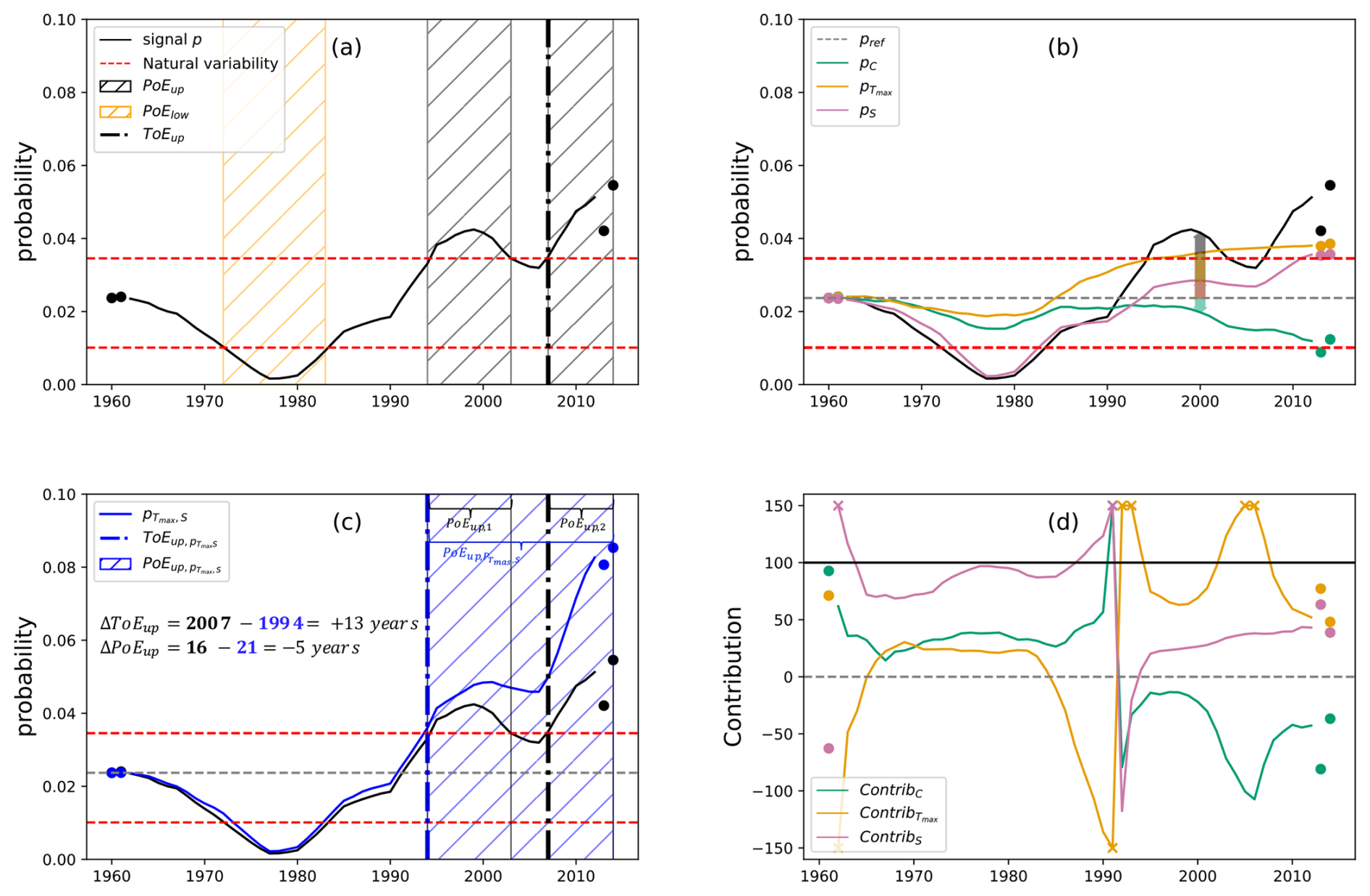
Figure 1 Illustration of the different steps used for characterizing the emergence (PoE, ToE, Contrib, ΔPoE_length, ΔToE_date), through the example of hot-dry CE in Vilnius. See text for details. (a) Periods of emergence below the lower bound and above the upper bound of the natural variability, given by the two dotted red lines, are shown with yellow and black hatched rectangles. (b) CE probability signals when only one component ($F_{T_{max}}$, F_S, C) changes. The computation of contribution is illustrated with the arrows. The difference between the signal p in 2000 and the probability during the reference period p_ref is represented with the black arrow (ΔP). The coloured ones refer to the differences between each time series p_C, ${\mathit{p}}_{{\mathit{T}}_{\mathbf{max}}}$, p_S in 2000 and p_ref. Panel (c) shows in blue the signal ${\mathit{p}}_{{\mathit{T}}_{\mathbf{max}}\mathbf{,}\mathit{S}}$ when the dependence is constant, and the associated PoE and ToE. By comparing (a) and (c), the two metrics ΔPoE_length and ΔToE_date can be computed. (d) Evolution of each component's contribution to the CE probability change (ΔP). CE probability and contributions associated to a change in the dependence, in the temperature index T_max, and in the drought index S are coloured respectively in green, orange and pink. The year indicated on the x axis is the middle of the 20-year window. All signals are smoothed using a 5-year window; thus the 2 first and 2 last years cannot be used for smoothing, and are plotted with points.

3 Marginals and dependence contribution to the emergence

Relying on the copula modelling, the CE probability is a combination of two marginal distributions, and a dependence function (Eq. 2). Thus, it can vary in time due to a change in margins and/or in the dependence structure. Which component change (marginal F_X, marginal F_Y, copula C) contributes the most to the change in CE probability during an emergence (ToE and/or PoE)? How does the dependence variation influence PoE features? Thanks to the decomposition of the signal (Eq. 2), each component can be modelled separately and the analysis of their respective evolution and contribution can be performed.

3.1 Contribution of changes in marginals and dependence to probability signal

In the copula-based formulation, it is possible to compute the probability of a specific event over a given period by assuming that only one component (e.g., F_X) has changed since the reference period, while the two other components (e.g., F_Y and C) remain unchanged, as they were in the reference period. Let us denote the CE probability as p_X when only F_X evolves; p_Y when only F_Y evolves; and p_C when only the copula C evolves. All three probabilities can be compared to p of the period of interest in order to quantify the different contributions. Let us take $p_{X_t}$, at time t (middle of a specific 20-year period), to understand in details how it is computed. The exceedance probability $p_{X_t}$, associated solely with changes in F_X, is computed by fitting the marginal F_Y and the copula C to the reference period ($F_{Y_{\mathrm{ref}}}$ and C_ref), while the F_X is fitted using the data from the period of interests ($F_{X_t}$). Then $p_{X_t}$ can be expressed as :

$$\begin{array}{}\text{(6)}& p_{X_t}=\mathrm{1}-F_{X_t}\left(x_e\right)-F_{Y_{\mathrm{ref}}}\left(y_e\right)+C_{\mathrm{ref}}\left(F_{X_t}\left(x_e\right),F_{Y_{\mathrm{ref}}}\left(y_e\right)\right).\end{array}$$

The probabilities $p_{Y_t}$ and $p_{C_t}$ are found in the same way, by changing the functions F_X, F_Y and C.

Now, in order to quantify the change in probability between the reference period and a period at time t, let us note Z, one of the three components $(Z\subset \mathit{\{}X,Y,C\mathit{\left\}}\right)$. CE probability changes when all the components evolve or when only Z evolves are noted ΔP and ΔPZ respectively, and expressed as:

$$\begin{array}{}\text{(7)}& \begin{array}{l}\mathrm{\Delta }P{Z}_t=p_{Z_t}-p_{\mathrm{ref}},\text{and}\\ \mathrm{\Delta }{P}_t=p_t-p_{\mathrm{ref}}.\end{array}\end{array}$$

We define the “Contribution” metric of the component Z at time t as the percentage of ΔPZ_t in ΔP_t:

$$\begin{array}{}\text{(8)}& {\text{Contrib}}_{Z_t}={\displaystyle \frac{\mathrm{\Delta }P{Z}_t}{\mathrm{\Delta }{P}_t}}\times \mathrm{100}.\end{array}$$

It allows us to quantify the proportion of change in the CE probability that is attributable to the change in the component Z.

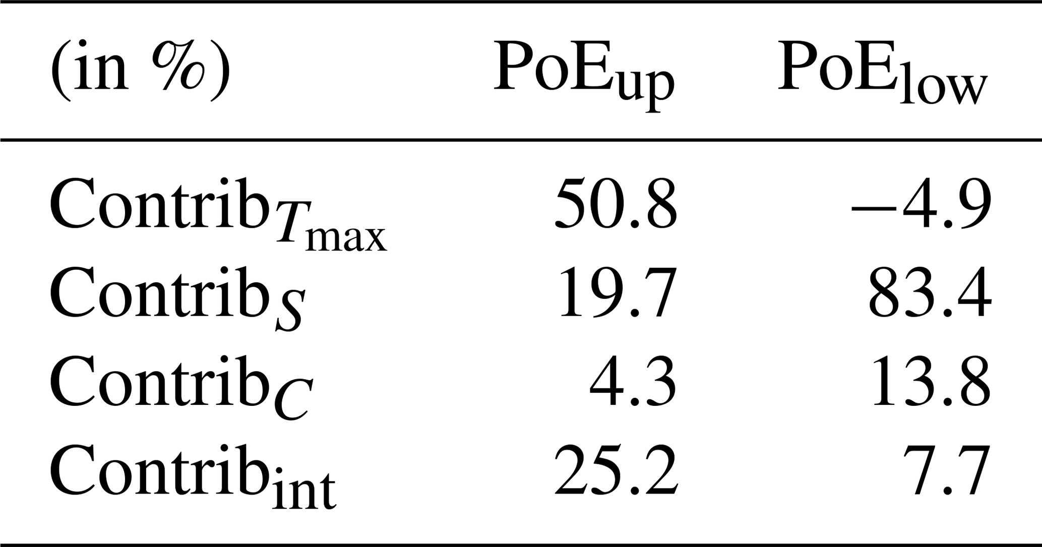
To highlight the contribution of each component during PoEs (i.e., when significant changes are detected), ΔPZ and ΔP are averaged over years that are part of PoEs. The total duration of PoE_up is noted N, and the contribution of Z over these years, Contrib_Z,up is expressed as:

$$\begin{array}{}\text{(9)}& {\text{Contrib}}_{Z,\mathrm{up}}={\displaystyle \frac{\stackrel{\mathrm{‾}}{\mathrm{\Delta }PZ}}{\stackrel{\mathrm{‾}}{\mathrm{\Delta }P}}}\times \mathrm{100},\end{array}$$

with

$$\begin{array}{}\text{(10)}& \begin{array}{l}\stackrel{\mathrm{‾}}{\mathrm{\Delta }PZ}=\frac{\mathrm{1}}{N}\sum _{t\in {\mathrm{PoE}}_{\mathrm{up}}}{p}_{Z_t}-p_{\mathrm{ref}}\\ \text{and}\stackrel{\mathrm{‾}}{\mathrm{\Delta }P}=\frac{\mathrm{1}}{N}\sum _{t\in {\mathrm{PoE}}_{\mathrm{up}}}{p}_t-p_{\mathrm{ref}}.\end{array}\end{array}$$

The simultaneous change in F_X, F_Y and C also contributes to the overall change of the signal. This contribution, called “interaction term” or “residual term”, is noted Contrib_int and is easily calculated as:

$$\begin{array}{}\text{(11)}& \begin{array}{l}{\text{Contrib}}_{\mathrm{int},\mathrm{up}}=\mathrm{100}-{\text{Contrib}}_{X,\mathrm{up}}\\ -{\text{Contrib}}_{Y,\mathrm{up}}-{\text{Contrib}}_{C,\mathrm{up}}\end{array}\end{array}$$

The metric Contrib_Z,up sums up the contribution of Z to the signal's emergence above B_up. If Contrib_X,up is higher than 50 %, the change in F_X mainly brings out the CE probability above the natural variability. It is easily transposable for lower-PoE in order to get Contrib_Z,low. The contribution metric is illustrated Fig. 1b and d, for the same example as in Fig. 1a. The evolution of the three probabilities (p_C, ${\mathit{p}}_{{\mathit{T}}_{\mathbf{max}}}$, p_S) is shown in Fig. 1b and their respective contribution is given Fig. 1d. The more the signal p_Z is close to p, the closer Contrib_Z will be to 100 %. During the lower-PoE, p_S follows the signal p, showing the high contribution of the component S during this period. ${\mathit{p}}_{{\mathit{T}}_{\mathbf{max}}}$ emerged above the natural variability before p, in 1995, T_max becomes the main driver during upper-PoE. Concerning the dependence, as the probability associated to the change of this component decreases until the lower bound of the natural variability, evolving in the opposite direction to p, its contribution during PoE_up is negative. Indeed, although the sum of the contributions is inherently equal to 100 %, individual contributions can be negative or exceed 100 %. This occurs because, for instance, two components may have opposing contributions of equal magnitude.

Bevacqua et al. (2019) approaches the notion of marginals and dependence contribution between two periods as a relative change: their metric was a ratio between a difference ΔPZ and a reference value and not a ratio of two differences. It has been applied either to return periods (Manning et al., 2019) or probabilities (Li et al., 2022) of compound events. If their contribution was equal to 1, it meant that p_Z doubled with respect to p_ref, but that does not place this variation within the total change, whose value we do not know. In our case, if the contribution is equal to 100 %, it means that p_Z has the same value as the probability p. Another difference relies on the sign of the contribution. If both signals p and p_Z decrease, the Bevacqua et al. (2019)'s contribution metric would be negative, while our contribution value would be positive as p behaves like p_Z.

3.2 PoE features influenced by a dependence change

Our contribution metric characterizes the effect of one component (marginals or dependence) change on the signal intensity during an emergence. However it gives no information about its influence on the date and duration of the signal emergences. The same difference between magnitude and time is retrieved between the metrics RR and ToE. That is why, in this part we will focus on the influence of a component change on PoE features, more specifically a change in dependence intensity. Indeed, Wang et al. (2021) highlights the importance of a stronger dependence in the increase of hot and dry events in several areas of the world between 1950 and 2017. Then, this section investigates how changes in dependence can affect the emergence of compound events probability.

Instead of analysing CE probabilities when a single component changes, only one (the dependence) will be kept constant and the two others will evolve. The signal p will be compared to p_(X,Y), when the copula is constant, while the marginals of X and Y change. p_(X,Y) at time t is expressed as:

$$\begin{array}{}\text{(12)}& p_{(X,Y{)}_t}=\mathrm{1}-F_{X_t}\left(x_e\right)-F_{Y_t}\left(y_e\right)+C_{\mathrm{ref}}\left(F_{X_t}\left(x_e\right),F_{Y_t}\left(y_e\right)\right).\end{array}$$

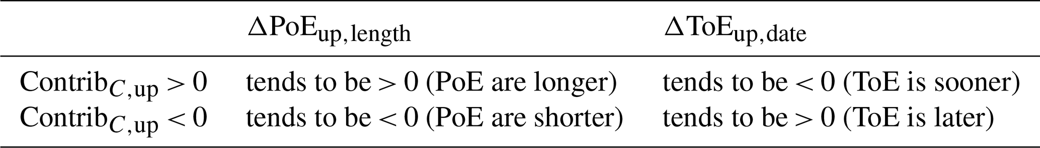
The difference between these two probability time series (p and p_(X,Y)) allows to quantify the influence of the non-stationarity of the dependence in the modelling. Two metrics are used in this section. The first one is defined as the difference between two ToE dates, detected on p and on p_(X,Y), noted ΔToE_date. When this metric is positive, p emerges later than p_(X,Y); considering the dependence change would delay the emergence of the signal p. In the same way, a negative ΔToE_date means that dependence variation tends to advance the permanent emergence of the signal. If the evolution of the component is not taken into account, ToE can be either under or over-estimated. The second metric concerns PoE and is defined as the difference between PoE duration identified on p and on p_(X,Y), noted ΔPoE_length. When this metric is positive, the signal p emerges either during a longer period or more frequently than p_(X,Y). A negative ΔPoE_length imply that p_(X,Y) is often higher than p; not considering the dependence change would overestimate CE probability and its emergence. Dependence can either contribute to increase or decrease the signal, to lengthen or shorten PoE, to advance or delay ToE. The link between these two metrics and the dependence contribution is summarized in Table 1 for upper-PoE.

Table 1 Summary of the link between three metrics, the contribution of the dependence during upper-PoE Contrib_C,up, the difference of PoE duration and ToE date when the dependence is considered or not, noted ΔPoE_up,length and ΔToE_up,date respectively: when the dependence contributes positively to the emergence of the signal, it means that the latter is higher when the dependence is considered, and tends to emerge sooner (ΔToE_up,date < 0) and more frequently (ΔPoE_up,date > 0). When the dependence contributes negatively to the emergence, it is the opposite.

As seen in Fig. 1d, dependence change contributes negatively to upper-PoEs in Vilnius. In Fig. 1c, the probability signal p (in black) is lower than ${\mathit{p}}_{{\mathit{T}}_{\mathbf{max}}\mathbf{,}\mathit{S}}$ when the dependence is constant (blue curve). The two vertical dotted-dashed lines show the shift in ToE when the dependence is considered or not: ${\mathit{p}}_{{\mathit{T}}_{\mathbf{max}}\mathbf{,}\mathit{S}}$ emerges 13 years sooner than the signal p (ΔToE_date is positive). Hence, for Vilnius, the emergence occurs earlier under the assumption of a constant dependence. Blue hatched periods in Fig. 1c can be compared with black hatched periods in Fig. 1a in order to visualize the metrics ΔPoE_length. The latter is negative and equal to −5 years, meaning that the PoE contains more years when the strength of the dependence is constant.

4 Results

The goal of this part is to shed light on spatial patterns of emergence over Europe and north Africa. To showcase a variety of mechanisms, five areas will be studied in greater depth. The latter were selected because signals tend to exhibit similar behaviors within each one. The delimitation is shown in Fig. 2: region MA-IB includes the Iberian Peninsula, the Maghreb, and south-west of France, region IT-BALK comprises south-east of France, Italy, and west part of Balkans, region EAST covers Western Ukraine, Eastern Poland, Eastern Slovakia and Southern Belarus, region NO-BALT consists of the countries along Northern and Baltic seas, and region LAP is located in northern Lapland.

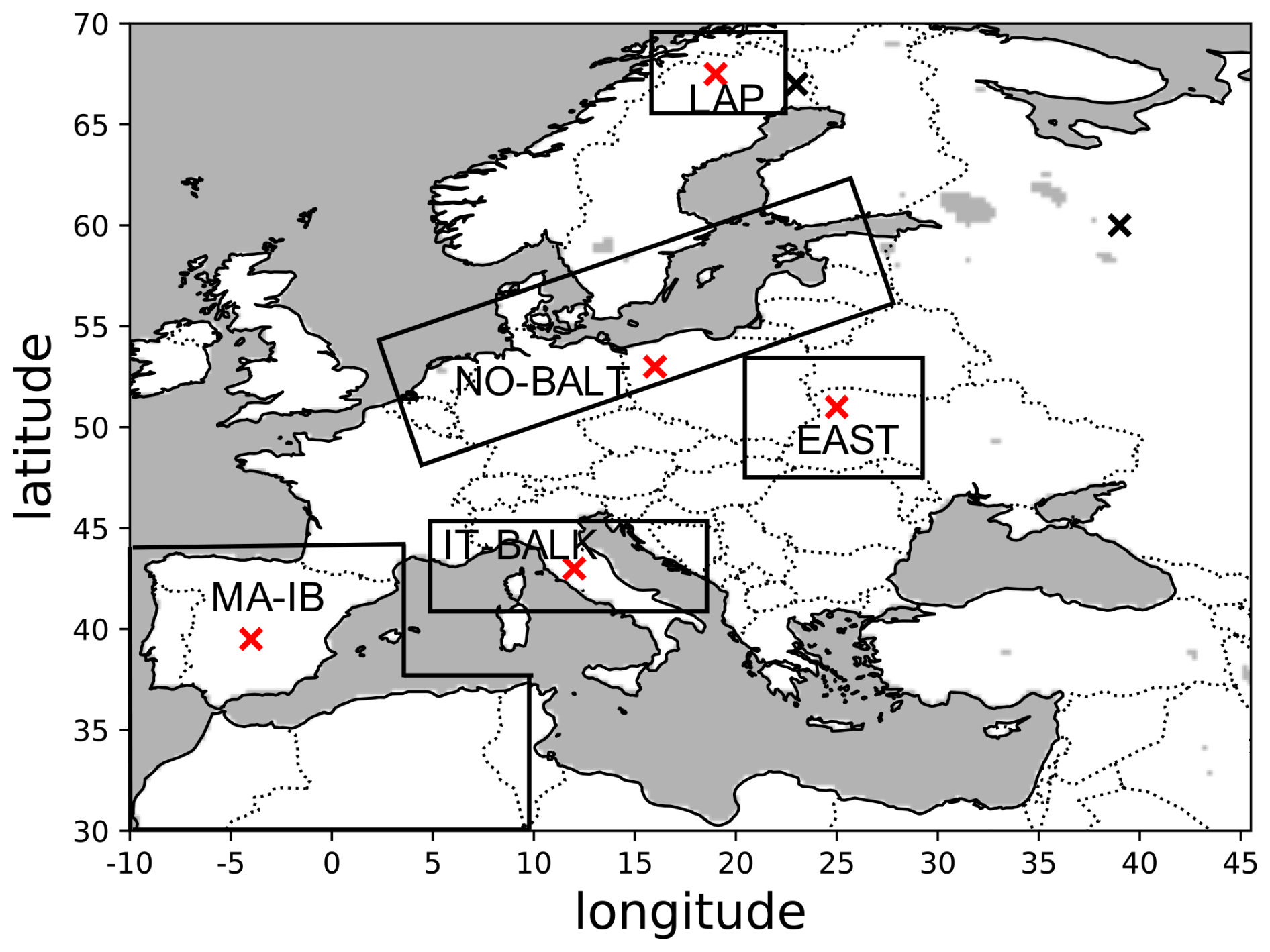
Figure 2 Presentation of the region under study and the five areas specifically analyzed: MA-IB (Iberian Peninsula, the Maghreb, and south-west of France), IT-BALK (northern Italy and western Balkan), EAST (western Poland, eastern Ukrain and southern Belarus), NO-BALT (zones along the north and Baltic seas), and LAP (northern Norwegian and Swedish Lapland). The red (black) crosses are the points specifically examined for the temporal analysis (in the Supplement).

The univariate thresholds $T_{{max}_e}$ and S_e correspond to the 95th percentile of the data during the reference period (Fig. S2). A strong gradient along latitude appears for the temperature: $T_{{max}_e}$ values in the countries along Mediterranean and Black seas are above 35 °C, $T_{{max}_e}$ values in Great Britain and in Scandinavia are below 30 °C, for the rest, $T_{{max}_e}$ range between 30 and 35 °C. For drought threshold, the values are closer through Europe during the reference period. This hot and dry compound event is centennial to millenial depending on the area (Fig. S3). The selected distributions for the two marginals and the copula, needed to compute the probability signal, are displayed in Fig. S4.

4.1 PoE features over Europe

Spatial patterns of emergence are presented Fig. 3. Hot and dry events occurrences emerged in most part of Europe and North Africa. 78 % of the grid points show an upper-ToE (colored points in Fig. 3a) and 4 % show a lower-ToE (colored points in Fig. 3b). In other words, 18 % of the grid points exhibit neither a ToE_up nor a ToE_low, suggesting that at these locations, the signal ultimately returns within the range of natural variability. The 18 % correspond to the white areas in Fig. 3a (no significant permanent rise), excluding the few colored pixels visible in Fig. 3b (significant decrease). The soonest ToE_up occurred in the region MA-IB, in Scandinavia and in Russia, which means that they have been affected by a significant increase of compound hot and dry events for several decades (Fig. 3a). In the whole MA-IB area, ToE_up is detected very early, even before 1970, in contrast to Scandinavia where CE occurrence do not evolve similarly over the region. In Ireland and in the eastern region (EAST), the probability has significantly decreased until the end of the study period, as shown by the coloured pixels Fig. 3b. Results of ToE can be compared to risk ratio (RR) values (Fig. S3). In MA-IB, where ToE is early, RR is the highest above 30. However in Scandinavia, RR is lower but ToE happened as early.

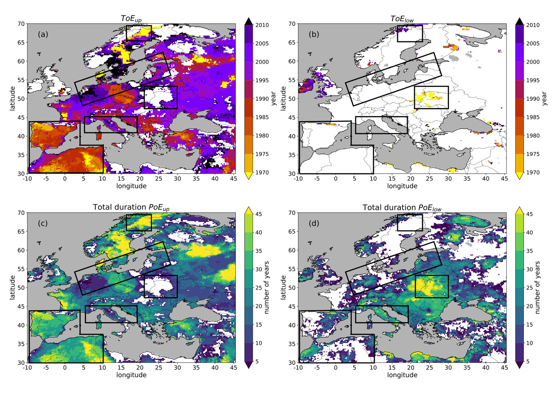
Figure 3 Maps of emergence features, when the signal varies below (b, d) or above (a, c) the natural variability. Date of (a) upper-ToE and (b) lower-ToE. Total duration of (c) upper-PoE and (d) lower-PoE. Maps (a) and (b) highlight the spatial patterns of time of emergence. In most of Europe, the probability signal has emerged above the range of natural variability by the end of the dataset. In contrast, some regions show a significant recent (Ireland) and old (Eastern Europe) decrease in CE probability. White areas in these maps indicate the absence of ToE_up (a) and ToE_low (b). Maps (c) and (d) identify hotspots of periods of emergence, showing where significant increases (PoE_up) or decreases (PoE_low) have occurred over the study period. White areas in these maps indicate the absence of PoE_up (c) and PoE_low (d).

As expected, maps representing ToE_up and PoE_up (Fig. 3a and c) look similar. The sooner the ToE_up, the longer the PoE_up. The differences between both maps lie in the number of PoE_up (Fig. S5). In North West of France, in Russia and in Scandinavia, several (between 2 and 4) upper-PoE occurred. Scandinavia looks more homogeneous in terms of PoE durations compared to ToE date (Fig. 3a and c). In the British Isles, Fig. 3c gives the information that in the past, the area recorded a significant rise out of the natural variability in CE probability, but from Fig. 3a and b we know that today the frequency is stabilizing or even decreasing. When a PoE_low appears, in 67 % of the time, the period lasts more than 10 years (Fig. 3d). The EAST region stands out from the others with a very long PoE_low, which is also highlighted on ToE_low map (Fig. 3b). Then, this area experienced a temporary (sometimes permanent) change of CE probability lower than the natural variability.

4.2 Marginals and dependence contribution to PoE over Europe

What drives these emergences? Figures 4 and 5 show the maps of each component contribution for upper-PoE and lower-PoE respectively. In general, marginals contribute mostly to the significant variations of the signal. On one side, T_max appears the main driver for upper-PoE (Fig. 4a). This is in line with Manning et al. (2019) and Shan et al. (2024) who found that the increase in temperature contributes predominately to the growing number of hot and dry compound events over Europe between 1950 and 2013 and in Belgium between 1901 and 2020. On the other side, the variable S is the primary contributor during lower-PoE (Fig. 5b). The spatial average of each component's contribution during lower and upper PoE is summarized on Table 2.

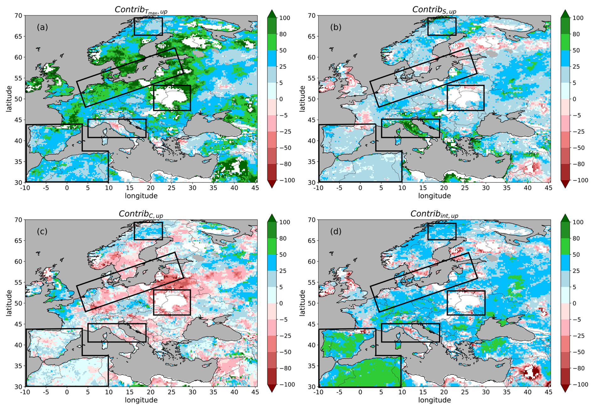
Figure 4 Contribution of each statistical component (T_max and S marginals, and the dependence C) during upper-PoE. Spatial patterns of (a) Contrib${}_{T_{max},\mathrm{up}}$, (b) Contrib_S,up, (c) Contrib_C,up and (d) Contrib_int,up. The last map corresponds to the residual term or interaction term. The sum of the four panels is equal to 100 (unit in %). White areas indicate regions where no PoE_up occurred. The contribution metric allows to identify which component change is most responsible for the significant increase in compound event probability. In most of Europe, T_max is the dominant driver. S is the main contributor only in Italy, though it remains positive across almost all regions. The dependence component shows regional contrast – it contributes positively in the west, but negatively in Eastern Europe. Finally, the residual term is the dominant factor in the Iberian Peninsula.

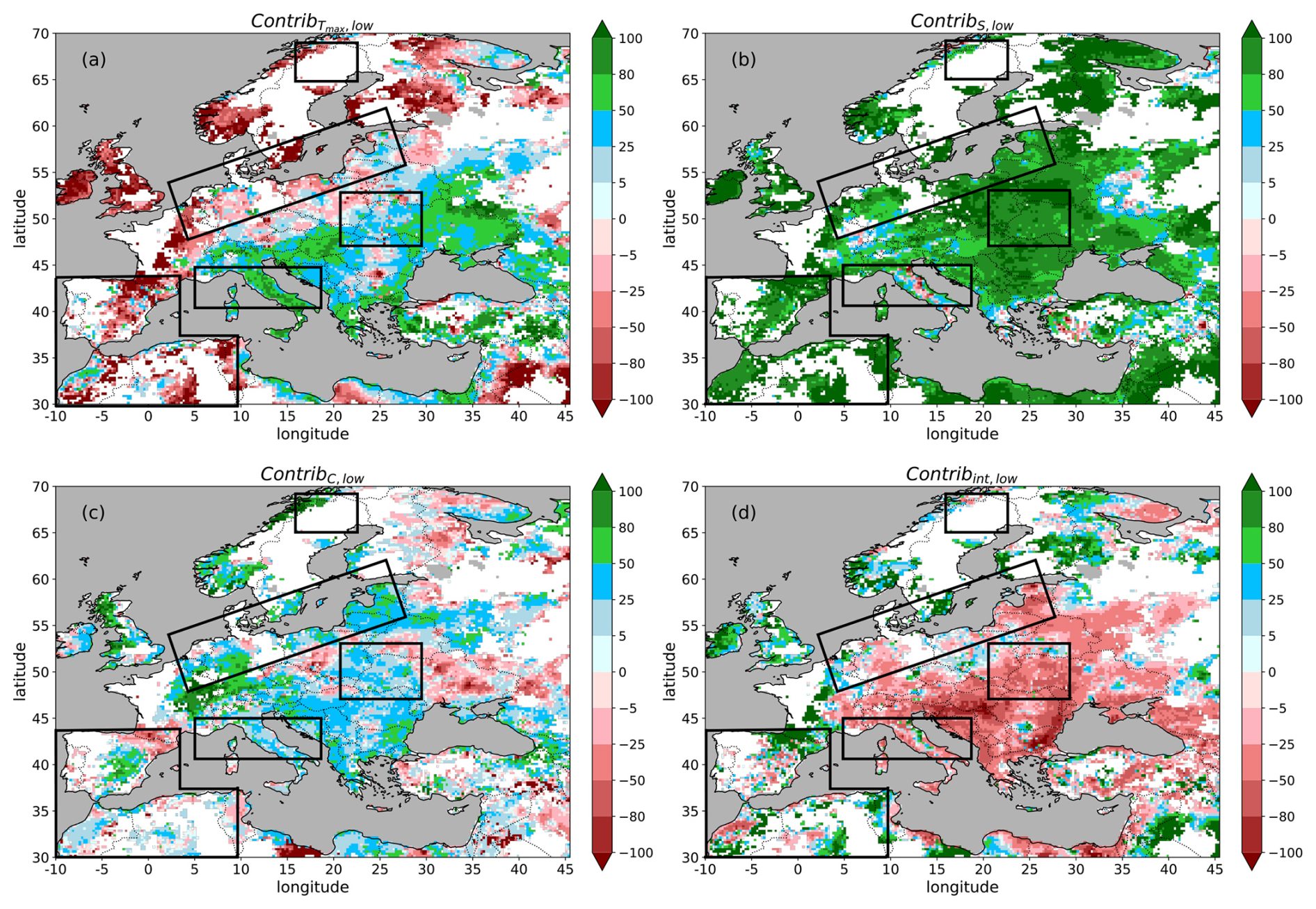
Figure 5 Contribution of each statistical component (T_max and S marginals, and the dependence C) during lower-PoE. Spatial patterns of (a) Contrib${}_{T_{max},\mathrm{low}}$, (b) Contrib_S,low, (c) Contrib_C,low and (d) Contrib_int,low. The last map corresponds to the residual term or interaction term. The sum of the four panels is equal to 100. (unit in %). White areas indicate regions where no PoE_low occured. The contribution metric allows to identify which component change is most responsible for the significant decrease in compound event probability. In most of Europe, S is the dominant statistical driver. T_max is the main contributor in Italy, Hongry, Ukraine, Greece and Turky. Contribution of the dependence change is mainly positive for lower-PoE, contrasting with the residual term which is highly negative.

Table 2 Spatial average of each component (the heat index T_max, the drought index S, and the dependence C) contribution during upper-PoE and lower-PoE (respectively Contrib${}_{T_{max}}$, Contrib_S, Contrib_C). Contrib_int is the residual term.

In 40 % of the time, mostly in NO-BALT area, temperature index explains a large part of the increase of CE probability (Fig. 4a). In this area the dependence contributes negatively to upper-PoE (Fig. 4c), which means that p_C evolves in the opposite direction to the signal p. In MA-IB area, T_max contributes positively around 30 % to PoE_up, twice the value of the drought index contribution (Fig. 4b). In this region, values of contribution are again homogeneous, those for dependence are close to zero (Fig. 4c) – it means that copulas show little change during the emergence – whereas those for the interaction term is the highest (Fig. 4d). The drivers are not the same during lower-PoE (Fig. 5). In 87 % of the time, drought index is mainly responsible of the signal variation below the natural variability (Fig. 5b). In these areas, mostly located in eastern Europe, the contribution of the dependence is positive (Fig. 5c). The IT-BALK region stands out in the sense that the drought index change is the main contributor to upper-PoE (Fig. 4b) while the temperature index plays this role for lower-PoE (Fig. 5a).

Signals p_S and ${\mathit{p}}_{{\mathit{T}}_{\mathbf{max}}}$ represent the CE probabilities when only the drought index and the hot index evolves respectively. Spatial patterns of their ToE and PoE are shown in Figs. S6 and S7 and provide another overview of the contributions. Probability signal ${\mathit{p}}_{{\mathit{T}}_{\mathbf{max}}}$ definitively emerged everywhere except in Italy and in Lapland whereas p_S definitively emerged in less than 50 % of the grid cells. To understand in details what happened during a period of emergence, the probability signal of five points, located in the five areas, are shown in Fig. 6. Their coordinates are represented with a red cross in Fig. 2. p_C (the green curve) does not change significantly as the probability remains in the range of natural variability, except in Lapland (Fig. 6e). For the EAST point (Fig. 6a), hot and dry probability is lower than during the reference period, despite the emergence of ${\mathit{p}}_{{\mathit{T}}_{\mathbf{max}}}$ (orange curve). For the IT-BALK location (Fig. 6b), the probability when only the drought index evolved, p_S (pink curve), emerged around 1990 and contributed in majority to PoE_up. Then for the MA-IB grid cell (Fig. 6c), the probability signal emerged in 1986, after the signal ${\mathit{p}}_{{\mathit{T}}_{\mathbf{max}}}$ and before p_S. For the NO-BALT point (Fig. 6d), ${\mathit{p}}_{{\mathit{T}}_{\mathbf{max}}}$ lies permanently above the natural variability since 1985. In the grid cell located in Lapland (Fig. 6e), the signal p emerges the soonest, around 1970, although ${\mathit{p}}_{{\mathit{T}}_{\mathbf{max}}}$ and p_S are almost constant. Contribution evolutions (Fig. S8) allow to better visualize how and when each component contributes to the variation of the probability signal, and to detect if the main driver changed from one period to another. The predominant role of T_max increase in NO-BALT area is highlighted in Fig. S8d. In the Lapland point (Fig. S8e), the main contributor alternates between margins and dependence change. Two more cases, located in Lapland and in Russia (black points in Fig. 2), are presented in Supplement (Fig. S9). In Lapland (23° E/67° N), the first PoE_up is mostly due to a change in the marginals whereas from 1985, dependence change became the main contributor; the opposite happens in Russia, marginals explain mostly the last PoE_up while dependence impacted the first one.

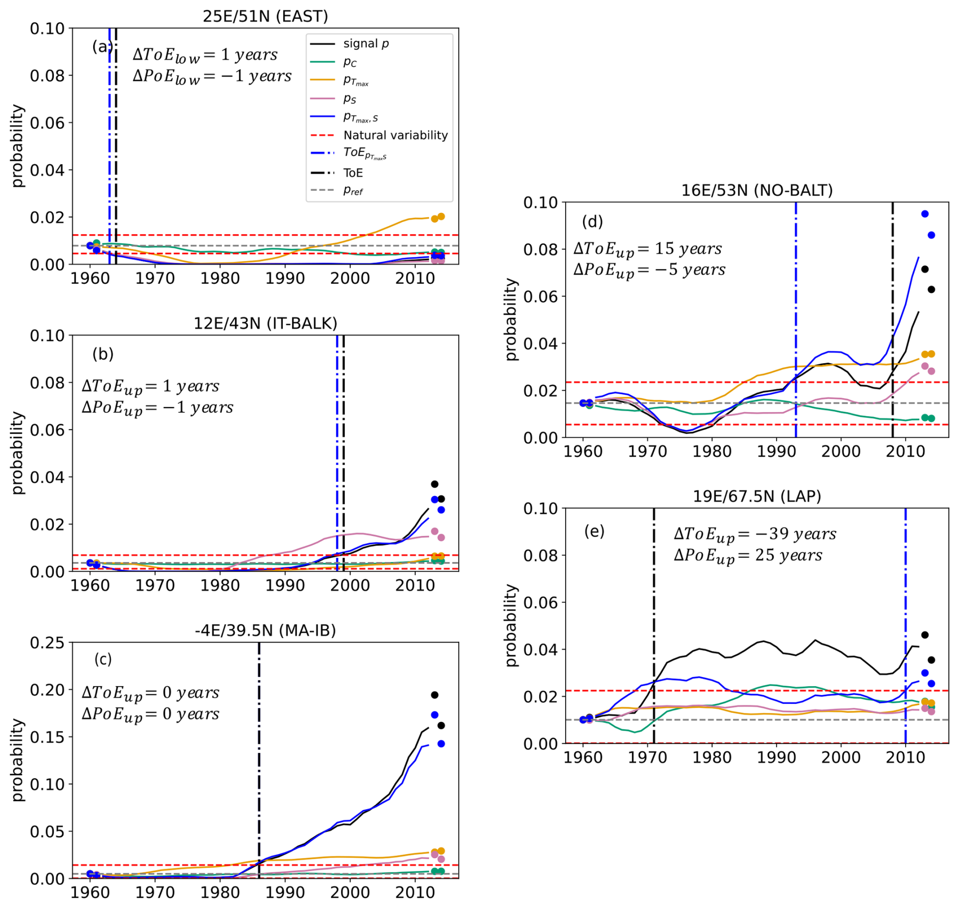
Figure 6 Evolution of hot-dry CE probabilities: when only one statistical component evolves, when the dependence is kept constant and the final signal p, at 5 points located in the 5 areas under study. Locations are given in Fig. 2 by red crosses. The probability associated with changes of dependence, temperature index T_max, and drought index S are coloured respectively in green, orange and pink. CE probability when the dependence is constant (${\mathit{p}}_{{\mathit{T}}_{\mathbf{max}}\mathbf{,}\mathit{S}}$), and the probability signal p are shown in blue and black. The year indicated on the x axis is the middle of the 20-year window. All signals are smoothed using a 5-year window; thus the two first and two last years cannot be used for smoothing, and are plotted with points. These graphs illustrate both the timing and magnitude by which the probabilities from different experiments emerge from natural variability. The vertical lines represent the time of emergence for the signals p (in black) and ${\mathit{p}}_{{\mathit{T}}_{\mathbf{max}}\mathbf{,}\mathit{S}}$ (in blue). In some cases, the interval between these two ToE is large (e.g., panels d and e), while in others it is nonexistent (e.g., panel c).

4.3 Influence of the dependence on PoE features

Although the dependence change is weaker and contributes less to the emergence than both margins variation, by how much does it impact the time and duration of the emergences? This section will compare two time series, the probability signal p and ${\mathit{p}}_{{\mathit{T}}_{\mathbf{max}}\mathbf{,}\mathit{S}}$, the CE probability when only both margins evolve, in order to quantify the influence of the dependence change on PoE features with the two metrics presented Sect. 3, ΔPoE_length and ΔToE_date. We will only focus on upper-PoE cases.

In Fig. 6 these two probability signals p and ${\mathit{p}}_{{\mathit{T}}_{\mathbf{max}}\mathbf{,}\mathit{S}}$ are represented in black and blue respectively. In Fig. 6c (MA-IB), when the signals overlap, both metric ΔPoE_length and ΔToE_date are equal to 0. In Fig. 6d (NO-BALT), ${\mathit{p}}_{{\mathit{T}}_{\mathbf{max}}\mathbf{,}\mathit{S}}$ is much higher than the signal p. The dependence between variables tends to decrease exceedance probabilities, since it contributes negatively to the emergence (as shown in Fig. S8c). As ${\mathit{p}}_{{\mathit{T}}_{\mathbf{max}}\mathbf{,}\mathit{S}}$ emerges sooner than the signal p, ΔToE_up,date is positive and reaches +15 years. As ${\mathit{p}}_{{\mathit{T}}_{\mathbf{max}}\mathbf{,}\mathit{S}}$ lies more often above the natural variability, ΔPoE_length is negative (equal to −5 years). On the contrary, in Fig. 6e (LAP), the probability signal p exceeds ${\mathit{p}}_{{\mathit{T}}_{\mathbf{max}}\mathbf{,}\mathit{S}}$ since p emerged in 1971, 39 years sooner than the ToE of ${\mathit{p}}_{{\mathit{T}}_{\mathbf{max}}\mathbf{,}\mathit{S}}$. In this case, contributions of the dependence and the margins are close, but ΔToE_date is highly negative and ΔPoE_length reaches +25 years.

This analysis points the diversity of ${\mathit{p}}_{{\mathit{T}}_{\mathbf{max}}\mathbf{,}\mathit{S}}$ evolution relative to the signal p. The two metrics are applied to each grid point of Europe and north Africa, ΔToE_date and ΔPoE_length spatial patterns are presented in Fig. 7. In MA-IB, ΔToE_date is close to 0, and ΔPoE_length around 2. NO-BALT stands out with high positive ΔToE_date. In Brittany and in Russia, the positive influence of the dependence is more pronounced for ΔPoE_length than ΔToE_date, as it corresponds to areas with several PoE_up (Fig. S5). In Lapland, the dependence influenced more the last PoE_up, so ToE_up is more impacted.

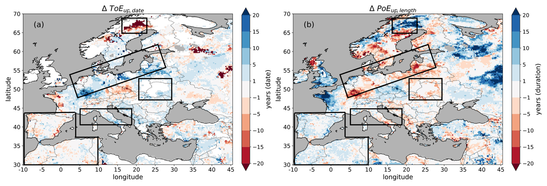
Figure 7 Influence of the dependence change on PoE features: either (a) on the upper-ToE date or (b) on the upper-PoE durations. When the dependence is considered, ToE can be advanced (negative ΔToE_date) or delayed (positive ΔToE_date), PoE can be longer and more frequent (positive ΔPoE_length) or shorter and rarer (negative ΔPoE_length).

4.4 A specific event: July 2022

The event studied so far corresponds to the combination of extreme temperature and drought (95th percentile during the reference period) whose thresholds do not refer to an observed event. That is why we will now focus on an event that happened in Europe and whose damage is documented. From now on, the selected bivariate thresholds $(T_{{max}_e},S_e)$ to compute the probabilities will correspond to the ERA5 values of a specific event. Hot and dry event in 2022 was particularly disastrous over Europe (Tripathy and Mishra, 2023). This phenomenon has drawn attention for numerous studies, such as the specific atmospheric circulation of the event (e.g., Faranda et al., 2023; Herrera-Lormendez et al., 2023), a particular attribution analysis (Bevacqua et al., 2024a), its impact on forests (Gharun et al., 2024) or on human death (Ballester et al., 2023). Summer 2022 has also been analysed on one side as an extreme heatwave (Feser et al., 2024) and on the other side as an extreme drought (Biella et al., 2025). What threshold does this hot and dry compound event correspond to? How likely was it to occur in the past compared to now? Is this likelihood emerged everywhere?

Regarding the corresponding thresholds (i.e., ERA5 values) for this event (Fig. S10), $T_{{max}_e}$ reached 45 °C in MA-IB (even higher in Northern Africa) and ranged between 40 and 45 °C over Europe (except Fennoscandia); and droughts were severe to extreme (S_e > 1.5 or 2) in a large part of the studied area. Their corresponding probability during the reference period (Fig. S10c and d) is not the same everywhere, this will impact the interpretation of the contribution maps (Figs. S11 and S12). For example, in the south of Sweden, $T_{{max}_e}$ is extremely high, above 30 °C, whereas S_e is even below 1. The likelihood of the hot index exceeding $T_{{max}_e}$ is around 10⁻⁴ while the probability of the drought index exceeding S_e is 10⁻¹. Then the joint exceedance probability signal is driven by the variation of T_max extreme values. It then differs to what has been done so far with percentile-based thresholds. Figure 8 presents the probability of occurrence during the baseline period and the risk ratio between the first and the last period (1950–1969 and 2004–2023). The event was unlikely to occur in MA-IB and in western France during the baseline period. There is a positive gradient, from west to east: the probability was around 10⁻⁴ in eastern France and eastern Germany, between 10⁻³ and 10⁻² in central Europe, and 10⁻¹ in Ukraine and Russia (Fig. 8a). The risk ratio highlights a huge increase in probability even higher than 50 in Central Europe (Fig. 8b).

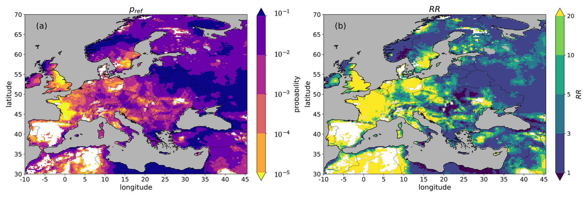
Figure 8 Probability during the reference period of the July 2022 hot and dry event and its associated risk ratio over Europe. (a) Probability of the event during the 1950–1969 period and (b) risk ratio (ratio of CE probabilities between the first period 1950–1969 and the last period 1994–2023). White grid cell refers to a null probability during the baseline period.

The probability associated to this event emerged almost everywhere, except in the EAST area and in the south of Norway (Fig. 9). This map, representing ToE_up, provides information on when the probability has increased significantly. In Ukraine and in Russia, ToE occurs after 2000, while the soonest ToE happens in Northern Algeria, Western Europe, Western Turkey and Southern Scandinavia. However this map has to be interpreted carefully, regarding map of p_ref (Fig. 8a). Indeed, in Spain for example, ToE means the moment at which the probability is no longer zero; whereas in Turkey, it refers to the time at which the probability is permanently above the estimated natural variability. This point is illustrated through two examples in Fig. 9b and c, in Northern France and in Poland.

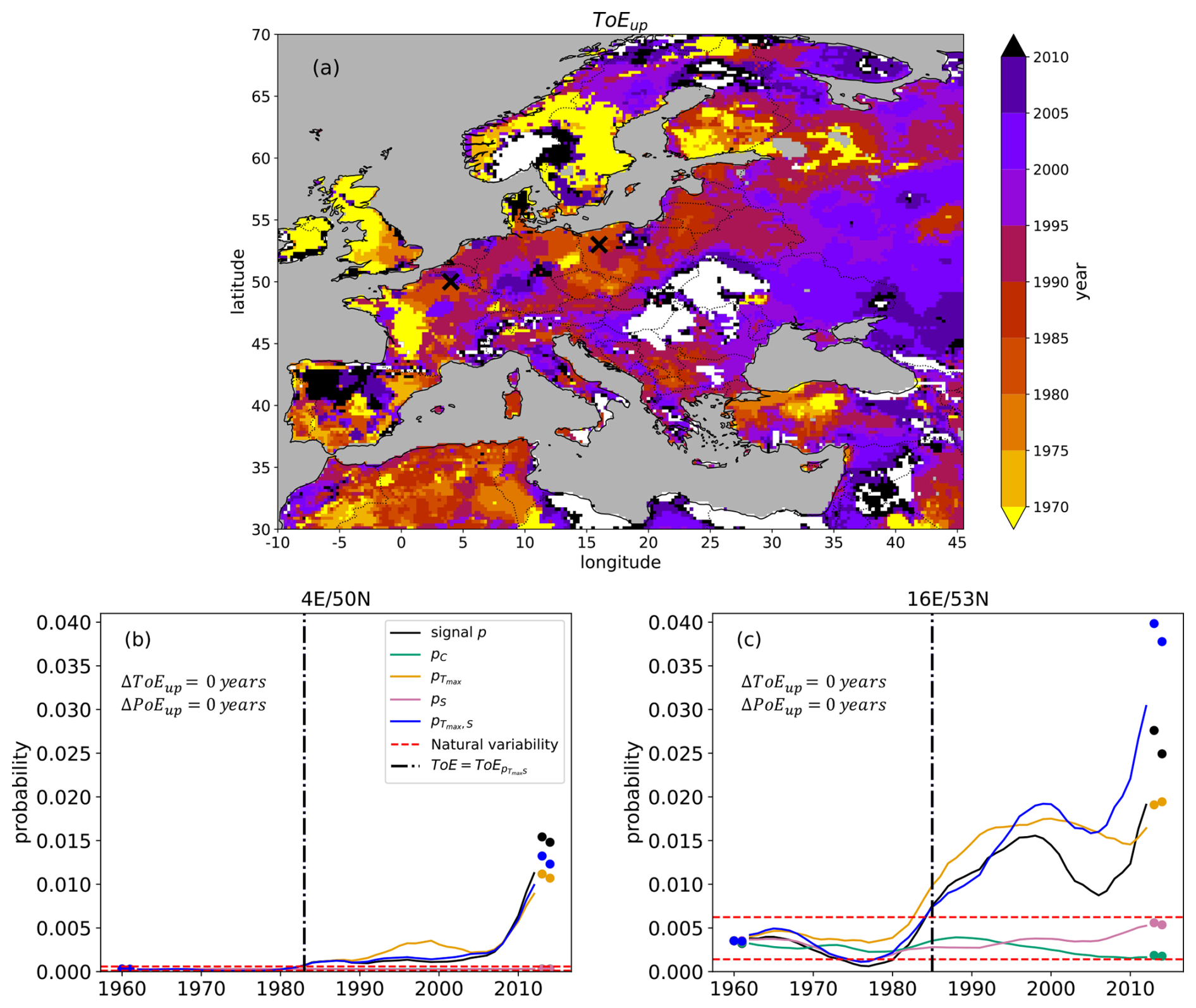
Figure 9 Time of emergence above the natural variability for the July 2022 hot and dry compound event. (a) Spatial distribution of upper-ToE. White grid cells indicate no upper-ToE detected within the study period (i.e., no significant and persistent increase in CE probability up to 2014). (b–c) Evolution of compound event probabilities at two specific locations, marked by black crosses in panel (a). These points are selected to illustrate two contrasting cases with similar upper-ToE: one with zero probability during the reference period (b), and another with greater natural variability (c). The probability associated with changes of dependence, temperature index T_max, and drought index S are coloured respectively in green, orange and pink. CE probability when the dependence is constant is shown in blue. The year indicated on the x axis is the middle of the 20-year window. All signals are smoothed using a 5-year window; thus the 2 first and 2 last years cannot be used for smoothing, and are plotted with points.

5 Conclusion and perspectives

5.1 Conclusion

Compound events are the most impactful phenomena. Changes in compound hot and dry event probability (signal) relative to the natural variability (noise) were detected in terms of timing and location. Time of emergence (ToE) is the year from which the signal goes out from the noise, while the new concept of period of emergence (PoE) refers to the periods during which the signal leaves the range of natural variability. This study analyses the evolution of the co-occurrence of extreme heat and drought and highlights the diversity of types of emergence over Europe and north of Africa between 1950 and 2023.

The signal permanently emerged above the natural variability in the majority of the area (78 % of the grid points show a time of emergence prior to the end of the temporal record). This implies a trend towards warmer and drier compound events. In order to better understand what happened in the past, periods of emergence were analyzed. In 65 % of the time, the signal experienced only one upper-PoE starting with a ToE. In some cases, the signal experienced an upper-PoE before the time of emergence, like in Scandinavia, Russia and Brittany (between 2 and 4 upper-PoE). In others, a lower-PoE occurred before, like in Italy. It is also interesting to detect areas where the signal never exceeds the upper bound, like in eastern Europe, or never evolve below the lower bound of the natural variability, like in Sweden, in Portugal and western Spain.

Temperature is the main driver for upper-PoE in most of Europe, while the drought index mostly contributes to lower-PoE (except in Italy). The magnitude of the dependence change is less significant, p_C almost never emerged permanently. Even if the dependence evolution is a low process, a few dependence variations can impact PoE features, either advance or delay ToEs, either lengthen or shorten PoEs. Sometimes, the main driver (among the three components) can change from one period of emergence to another.

Five areas were studied in detail, each characterized by their own specificity in terms of ToE, PoE, contributions and ΔPoE_length. The frequency of hot and dry events sharply increased in Maghreb and the Iberian peninsula (MA-IB), and this rise is mainly due to a change in the marginals. Conversely, in eastern Europe (EAST) the signal experienced a long lower-PoE, that can lead to a lower-ToE, and this decline is mainly driven by a change in the drought index. In northern Italy and western Balkan (IT-BALK), S contributes mostly to the emergence above the natural variability, and not below like the rest of Europe. Finally, the dependence change impacted Baltic states and Lapland differently. It influenced negatively the probability around the northern and Baltic seas (NO-BALT), which means that the signal is lower when copula parameter evolves, periods of emergence are shorter and time of emergence later. However, in Lapland (LAP), time of emergence could be delayed by 30 years if the dependence were not taken into account. The study highlights regional contrasts and specificities.

The study shows that the developed approach can be adapted to the analysis of a specific impactful CE (not only CE event based on climatology). As an example, July 2022 has been taken as a threshold. Indeed, this methodology can be applied to any bivariate compound event, with any bivariate threshold, and at any location. An R package has been developed, allowing to detect upper/lower PoE, upper/lower ToE, to visualize the time series of the probabilities p, p_C, ${\mathit{p}}_{{\mathit{T}}_{\mathbf{max}}}$, p_S and ${\mathit{p}}_{\mathbf{(}\mathit{S}\mathbf{,}{\mathit{T}}_{\mathbf{max}}\mathbf{)}}$, to detect their emergences and to quantify the contribution of the three statistical components. This package is available on https://github.com/josephine400/emergence.compound (last access: 11 December 2025).

All in all, this paper identifies hotspots of emerging hot and dry compound events (CEs) across Europe. Most regions show a permanent and significant increase in CE probability, while some areas such as Ireland and parts of Eastern Europe exhibit a significant recent and old decrease respectively. In most cases, increases in CE frequency are primarily driven by changes in the heat index, whereas decreases are mainly linked to variations in the drought index. Importantly, the study demonstrates that the statistical dependence between heat and drought is a key factor in detecting the emergence of compound events.

5.2 Limitations and perspectives

The emergence of a climate signal is a valuable impact indicator, as it marks the point when the signal exceeds natural variability – beyond which human and ecological systems are typically adapted. Compound events, especially those combining heat and drought, have severe impacts on society, water resources, and agriculture (Ribeiro et al., 2020). Therefore, identifying when, for how long, where, and to what extent the occurrence of these high-impact events has changed is of great interest to many communities. Stakeholders and farmers can benefit from such studies in designing adaptation strategies. For instance, Lesk et al. (2022) emphasize the importance of developing agricultural adaptation policies tailored to different spatial and temporal scales of hot and dry events.

This type of research is also valuable for climate physicists, hydrologists, and agronomists, who aim to understand the physical and physiological mechanisms underlying significant increases or decreases in these compound events. We analyzed how changes in statistical dependence affect the emergence of compound events. While it is well established that there is a physical link between heat and drought, particularly through land–atmosphere feedbacks (Miralles et al., 2014), it is essential to further explore how changes in statistical dependence reflect underlying physical processes. In terms of atmospheric drivers, Ionita and Nagavciuc (2021) demonstrated that hot and dry events across Europe are frequently associated with atmospheric blocking patterns. It would be valuable to connect statistical contributions with physical drivers: how might the spatial patterns of the contributions (of the three components forming the CE) relate to soil characteristics, oceanic influences, or atmospheric dynamics?

The method developed in this study is generic and applicable to any bivariate compound event. Changing the variables, spatial scale, or temporal resolution will naturally change the event probabilities and, in turn, highlight different patterns of emergence and contribution. Further analysis of other bivariate events, such as extreme precipitation and wind, or alternative representations of hot and dry conditions (e.g., minimum temperature with precipitation, or the number of hot days with SPEI3), across different spatial and temporal scales, could yield valuable insights for future research tailored to the needs of societal stakeholders.

The method is adaptable to any reference period. In this study, we used the 1950–1969 period for its early timing, stationarity, and limited global warming influence. Reference periods are often around 30 years (with reanalyses), and up to 50 years (with simulations). However, several studies have used shorter baseline periods, such as the 20-year window from 1980 to 1999 (Giorgi and Bi, 2009; Diffenbaugh and Sherer, 2011; Vrac et al., 2023). Diffenbaugh and Sherer (2011) found similar results for the global emergence of permanent, unprecedented heat in the 20th and 21st centuries when using either the 1980–1999 or 1951–1999 reference period. Zscheischler and Lehner (2022) even adopts a 10-year baseline period (1950–1969) for a compound event attribution study. Then other baseline periods (whether longer or set at different times) can be used to analyze the emergence of compound event probabilities. The choice of the reference period is crucial when interpreting detection results, as detection is inherently relative to this baseline. Changing the reference period can alter the estimation of natural variability, either narrowing or widening it, which in turn affects Periods of Emergence (PoE). This flexibility allows the analysis to be adapted to different research objectives.

The methodology developed here uses copula functions to disentangle univariate and dependence contributions during PoEs. The study is then limited to 2-dimension compound events. But spatial compound events or multivariate hazards described with more than two variables (like wildfires studied with wind speed, temperature and humidity) are other high-impact phenomena and need further multivariate statistics (e.g., Tavakol et al., 2020; Davison et al., 2012). This work would then deserve to be extended to higher dimensional events. Several approaches have been implemented to tackle this modelling issue. Nested Archimedean construction for example also called Hierarchical archimedean copula, introduced by Joe (1997) consists in inserting copula into copula. A tree structure of dependence is built to guide the computation (Ribeiro et al., 2020). Pair Copula Construction, also proposed by Joe (1997), deals also with more than 2 dimensions, by decomposing a multivariate distribution into multiple bivariate copulas (Manning et al., 2018). These methods allow to model more complex dependencies than a multivariate Archimedean parametric copula that imposes the same parameter for each pair of variables.

In the present study, CE probabilities are modelled by fitting marginal and copula distributions to the data of each sliding window. Then, a large portion of the same data is used several times from a sliding window to another. The signal modelling can be improved by considering more properly the non-stationarity, e.g. including physical covariates to condition the joint distribution, and by applying other bivariate methods, such as non-parametric approaches or multivariate generalized Pareto distribution (Legrand et al., 2023).

The ERA5 reanalysis dataset is analysed for the present case study in order to detect past changes. However the period is only available from 1950 to 2023. Using simulations from climate models can shed new lights on multivariate detection and attribution framework. Simulations provide access to longer datasets, enabling the analysis of extended PoE trends. They offer insight into how climate models represent natural variability compared to reanalysis data. Analysing simulations can be used to evaluate CMIP6 models ability to retrieve compound events emergence. If simulations detect the right frequency of PoE without the right main driver, the reliability of the model may be weakened. In addition to improve CE detection, models are needed for attributing a phenomenon to anthropogenic activities (e.g., Stott et al., 2016). For this purpose, compound event probabilities computed in two different periods are compared, either the present with the past (pre-industrial period) or a factual world with a counterfactual world (without anthropogenic forces) (Zscheischler and Lehner, 2022). The modelling and method proposed in this study could then be directly used for such a task.

Finally, as compound events are expected to change in the future (Ridder et al., 2022), the methodology presented in this study could be applied to climate model simulations for projection, in order to anticipate potential future significant CE probability variations (future PoE and ToE), and be as prepared as possible to these complex and devastating events.