
the Creative Commons Attribution 4.0 License.
the Creative Commons Attribution 4.0 License.
 | 17 Nov 2026
Present and future trends of extreme short-term rainfall events in Germany, by downscaling convective environments of ERA5 and a CMIP6 ensemble

Maik Heistermann
For the four main quadrant regions of Germany we study the possibility of projecting the occurrence of extreme convective rainfall events, as monitored by the CatRaRE database, into the future, based on CMIP6 projections of corresponding convective environments. We characterize such environments by using the atmospheric profile derivates convective available potential energy (cape) and convective inhibition (cin), along with model-simulated convective precipitation (cp). The convective environments are linked to the small-scale CatRaRE events by classifying the corresponding ERA5 fields according to the concurrent occurrence of such events. Classifiers are conventional machine-learning procedures along with more modern deep learning schemes. Positive centennial trends are identified for both antagonists cape and cin, serving as a source for large uncertainties of the corresponding CatRaRE-type trends. Their full distribution is analyzed using ANOVA, based on the factors of event severity, greenhouse gas emissions, climate models, classifiers, and region. Beyond all uncertainty, positive trends outweigh the negative ones for all regions.
- Article
(3227 KB) - Full-text XML
-
Supplement
(1282 KB) - BibTeX
- EndNote


Flash-floods are among the most destructive environmental hazards. The areas mostly affected are mountainous regions as well as urban agglomerations. As a result, flash-floods are for Germany the most costly type of extreme events, with an estimated cost of more than EUR 70 billion due to flood damages for the last two decades (Trenczek et al., 2022).
It is known that a warmer atmosphere can hold more water vapor (the so-called Clausius-Clapeyron (CC) law), giving rise to enhanced downpour once a heavy precipitation event is under way (CC scaling, cf. Fowler et al., 2021). There is also evidence of such downpour happening more often, even more so for the strongest events (Myhre et al., 2019). This pertains in particular to short-term heavy convective summerly rainfall that is typically the cause of flash floods. To quantify future impacts, climate models are increasingly being developed and applied at km-scale resolution, so called convection-permitting climate models, where deep convection is treated explicitly instead of being parameterized, resulting in a highly improved representation of convective precipitation (Fosser et al., 2020; Kendon et al., 2021; Lin et al., 2022; Lucas-Picher et al., 2021). These being computationally expensive, corresponding simulations remain limited and statistical estimations uncertain. To overcome such limitations, convection is sometimes emulated in climate models, using a whole spectrum of schemes ranging from simple parametric approaches to full-blown emulators driven by artificial intelligence (AI) (Gentine et al., 2018; O'Gorman and Dwyer, 2018); see also Ukkonen and Mäkelä (2019). More conventionally, a variety of empirical schemes known as “statistical downscaling” have been employed, with varying success, to obtain realistic heavy local rainfall patterns that are consistent with the large-scale atmosphere; for a more recent overview see Devadarshini et al. (2025). This is facilitated by using, for example, variables that describe the atmospheric conditions prone to convection – so called convective environments – and hence to heavy precipitation. This way, century-long projections of short-term regional or local future rainfall and correspondingly more stable statistics of rainfall extremes can be obtained (Bürger et al., 2019; Bürger and Heistermann, 2023), henceforth BH). Still, many questions remain unsettled regarding the interplay between (present or future) atmospheric convective environments and heavy local precipitation (Meyer et al., 2022).
For Germany, an inventory of extreme rainfall events has recently been compiled from more than 20 years of weather radar records (CatRaRE, cf. Lengfeld et al., 2021). In a first effort to project CatRaRE-type events into the future, BH applied a classification approach to downscale a single future simulation of the EURO-CORDEX suite. As classifiers, conventional statistical downscaling schemes were benchmarked against more modern AI-based models. Regardless of method, CatRaRE-type extreme events were projected to increase significantly throughout the century. This study is now extended in various directions: while BH had used a binary predictand (event/no event), this is now extended to include multivariate regional predictands as well as different event magnitudes. And most notably, instead of using a single model of the older CMIP5/CORDEX suite, here we use the new CMIP6 models directly, and we do so with as many of them as possible to obtain thorough uncertainty estimates of our results.
2.1 CatRaRE
The basis of CatRaRE is a 22-year (2001–2022) long record of hourly precipitation fields of 1 km resolution over Germany, which itself is derived from weather radar observations (Winterrath et al., 2018). From these precipitation fields, CatRaRE identifies spatio-temporally contiguous objects (events) in which rainfall exceeds warning level 3 (as defined by the Germany Meteorological Service). This threshold corresponds to 25 mm in one hour or 35 mm in 6 h. Each event is assigned a location and timestamp, using its centroid and mean of start and end date, respectively, as well as a set of additional metrics. One of these metrics is the extremeness index ET,A of Müller and Kaspar (2014), which combines area, duration and intensity measures. Focusing on convection, we select events that took place in the summer months May to August with a duration of at most 9 h, leaving a total of 20 824 cases. As a first glimpse, Fig. 1 displays our selection of CatRaRE events grouped into single years, along with the corresponding annual 99, 99.9, and 99.99 percentiles of ET,A and their trends. While the 99 percentiles show no trend (p>0.5), the extreme (99.9) and very extreme (99.99, equaling the maximum) percentiles reveal, with growing significance (p<0.02 and p<0.002, resp.), clear upward trends. We note that throughout the following, trends are estimated using linear (ordinary least squares) regression, and that in all cases corresponding residuals are consistent with this model (normality), so that trend lines and significance estimates are reliable. In the case above this is quite remarkable because, after all, we are looking at a measure of annual extremes of precipitation; it is a likely consequence of the integrating effect of that measure, the extremeness index ET,A. The Supplement contains an alternative approach via quantile regression, also revealing positive, albeit insignificant trends.
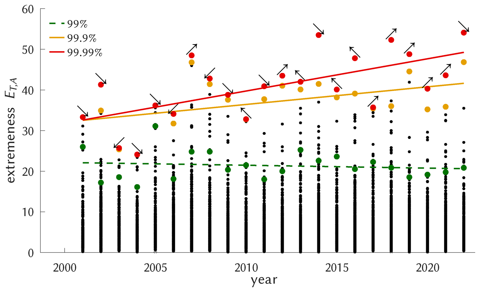
Figure 1For each year, all relevant CatRaRE events (≤ 9 h, May–August) are shown (black dots), along with their 99, 99.9, and 99.99 percentiles and corresponding regression trendlines (colored dots and lines) and p-values p≈0.6, p≈0.02, and p≈0.002. The arrows attached to the red dots point to the region quadrant of the respective event.
To further study these very extreme cases, we select events that have and , corresponding to the 90th and 99th percentiles and representing the 2040 and 208 strongest cases, respectively. The severity classes, denoted as P00 (all events), P90, and P99, respectively, should be sufficiently large to undergo the statistical modeling as described below.
2.2 Atmospheric data
We use observed (reanalyzed) atmospheric fields from ERA5 for the summer months of the years 1979–2022 (Hersbach et al., 2020) and corresponding fields as simulated for present (1960–2014) and future (2015–2100) by the current version of the Coupled Model Intercomparison Project (CMIP6), available on the Earth System Grid (https://pcmdi.llnl.gov/CMIP6, last access: 13 December 2024). As convective environments we use convective available potential energy (cape), convective inhibition (cin), and (model-simulated) convective rainfall (cp). As the name suggests, cape is a measure of the atmosphere's potential to freely develop convection between the level of free convection (LFC) and the equilibrium level (EL) where buoyancy stops. cin, on the contrary, measures the stability below: starting at the surface level (SFC), it quantifies the effort that is needed to reach LFC and hence initiate convection; a typical force for such upward movement are orographically forced or frontal updrafts. It follows that the local effect of cape is mostly on rainfall intensity while for cin it is on rainfall occurrence (or frequency). Both, cape and cin, are integral measures of the temperature and humidity profiles, basically measuring each level's contribution to the parcel's buoyancy.
The latter is essentially given by the relative difference of the parcel's virtual temperature and the virtual temperature of the environment, Tv,p and Tv,e, respectively, so that cape and cin are obtained from Eqs. (1) and (2):
As cape and cin are not provided by the CMIP6 models they had to be calculated from these profiles, following Bolton (1980). ERA5 provides convective environments, but for consistency, Eqs. (1) and (2) were also used for ERA5. Note, however, that upper-air measurements from observations are sparse, so that atmospheric profiles, from reanalysis or simulations, remain uncertain (Taszarek et al., 2021). Convective precipitation (cp) itself is provided by all models (Emmenegger et al., 2024).
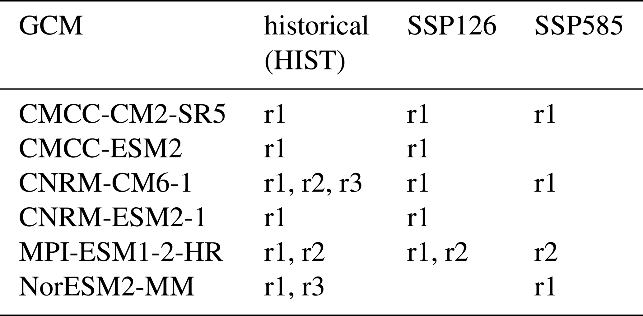
To capture uncertainty, we have attempted to obtain as many of the CMIP6 simulations as possible. Several limitations applied: because we use an anomaly approach (see below), respective reference (historical) simulations of the same model are required; furthermore, only models were used whose temporal resolution of the vertical profiles was at least 6-hourly, and cp was interpolated or aggregated to the same temporal resolution. Spatially, we allowed only models with an original resolution not coarser than 1.5 × 1.5°, and interpolated or aggregated their fields to a unique 10 × 10 grid between the corners [5.75° E 47.25° N] and [15.25° E 55.25° N]. A summary of all simulations is shown in Table 1. For any GCM, field variable, and severity level ξ, the reference climate was calculated as mean and standard deviation (μ,σ) across all grid points and historical realizations of the same GCM from the reference period 1981–2010; from that, standardized anomalies are formed to enter the classification. For the shallow methods all fields undergo, as in BH, an EOF reduction prior to the classification task, see more details in the Supplement.
Table 1Summary of CMIP6 simulations with realizations r1, r2, r3.
A typical constellation of ERA5 cape and the concurrent state of CatRaRE from 17 June 2001 is shown in Fig. 2. It was a day with strong atmospheric convectivity (cape > 700 J kg−1) that led to numerous heavy thunderstorms over Northeast Germany, including the cities of Hamburg and Berlin.
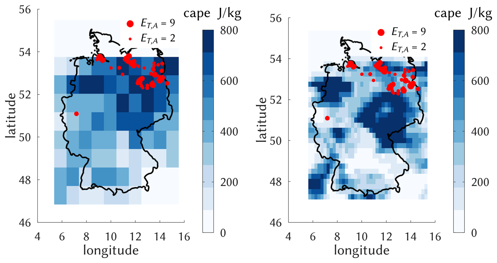
Figure 2Left: typical strong convective constellation on the afternoon of 17 June 2001, with a corresponding cape field at resolution 0.8 × 0.8, as calculated from ERA5 profiles using Eq. (1) (see text) and classified as a Northeast (NE) event; red dots indicate CatRaRE events and their extremeness ET,A, with . Right: the same situation with the original ERA5 resolution of 0.25 × 0.25 as used by BH.
2.3 Classification
In order to investigate whether any change in the frequency of heavy rainfall varies regionally within Germany, we subdivide the area of Germany into four quadrants (NW, NE, SW, SE), defined by maximum and minimum longitude and latitude coordinates and respective centers. Any 6 h interval d is now classified as belonging to
-
0, if no event exists whose timestamp falls into d;
-
R, if more than half of the events that fall into d lie within the region R, with ;
-
1, otherwise.
As an example, the 6 h-interval after 17 June 2001, 12:00 LT, pertaining to Fig. 2 is classified a NE extreme event. Note that no further distinction is made, for example, with regard to multiple, almost simultaneous events in a single quadrant. Note also that the classification depends on the particular shape of the German border although its small-scale details (an event might occur just outside Germany) have certainly no representation in the atmospheric predictor fields. This is the same kind of limitation that station downscaling shows in general, and cannot be avoided. The relative frequency of each of these 6 CatRaRE-based classes, in the following referred to as the class's base rate, are displayed in Table 2.
Table 2Base rate (in % of all events) for all classes (regions) under different percentiles.
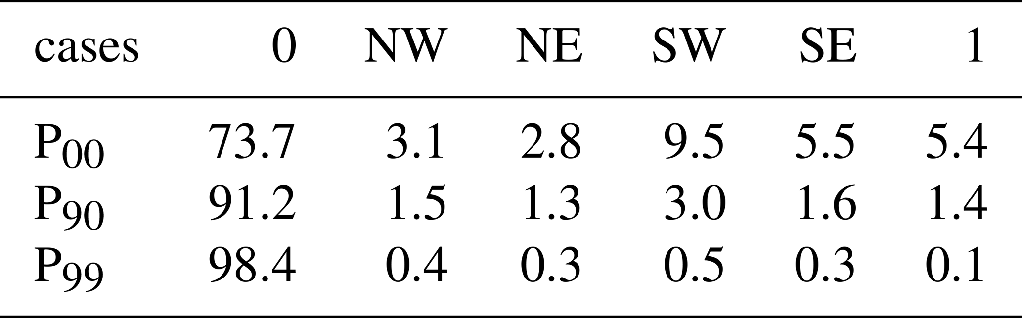
The focus of this study lies in estimating the evolution of these class rates through time, and specifically whether the rates are affected by climate change.
2.4 Conventional (“Shallow”) and Deep Learning models
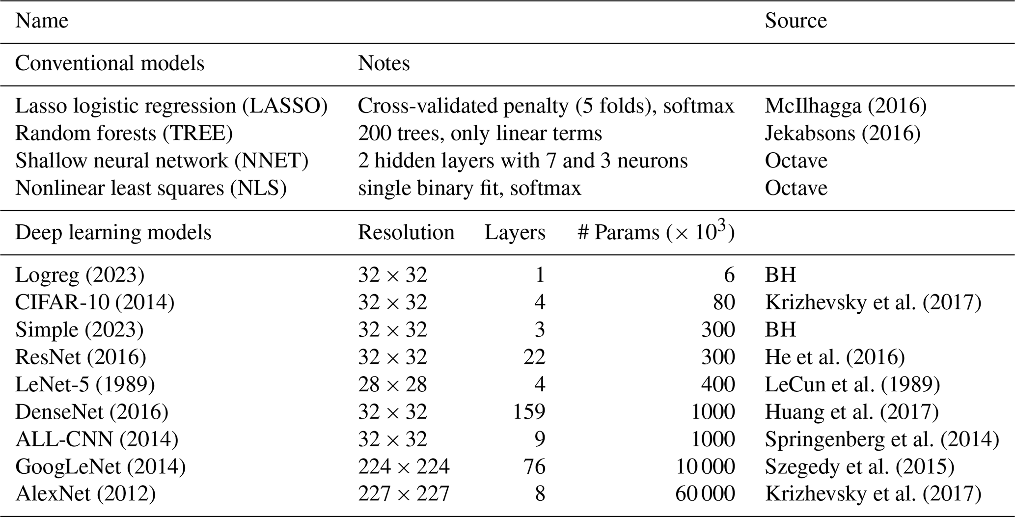
As classifiers, we employ two groups of empirical schemes, one using more conventional statistical or machine learning tools, and another representing deep learning (DL) neural networks. The DL network architectures are based on convolutional neural networks, a concept that was introduced with the famous LeNet-5 model of LeCun et al. (1989) for the classification of handwritten zip codes. While those numbers were coded on a 28 × 28 grayscale grid, the efforts quickly evolved into classifying high-resolution color images of cats and dogs and other increasingly complex objects from daily life. All networks of our selection had in its time excelled in the notorious ImageNet classification contest, cf. https://en.wikipedia.org/wiki/ImageNet (last access: 1 April 2025). By interpreting each instance of the atmospheric fields of cape, cin, and cp as the 3 color channels of an image, the networks can be used for the classification. More details are provided in the Supplement and BH, and a summary in Table 3.
McIlhagga (2016)Jekabsons (2016)Krizhevsky et al. (2017)He et al. (2016)LeCun et al. (1989)Huang et al. (2017)Springenberg et al. (2014)Szegedy et al. (2015)Krizhevsky et al. (2017)Table 3The conventional (“shallow”) and deep learning classifiers. The DL resolution is taken from corresponding images of typical applications, e.g. 32 × 32 from the CIFAR-10 dataset.
2.5 Exceedance counting
Prolonging the trends of Fig. 1 linearly into future decades would represent a quite simplistic projection of ET,A, concluding that, for example, the annual 99.99 percentiles grow from a starting level near ET,A = 30 to one of ET,A = 50 merely 20 years later, which amounts to a centennial trend of about 100 ET,A units. This approach is appealing but certainly not much more than heuristic. Our probabilistic classification scheme described above, instead, employs the full information contained in present and future convective atmospheric environments on a sub-daily basis. But such a scheme is incapable of deriving actual events with concrete values of ET,A, as displayed in Fig. 1. To relate class probabilities to Fig. 1, we show in Fig. 3 for the severity classes P90, P99, P99.9 (i.e. the all-time 90th-, 99th-, and 99.9th-percentiles) the corresponding annual exceedance counts. These quantities, in particular their centennial trends, are the target quantities for which this study provides future estimates. In Fig. 3 they are shown relative to their overall mean per severity class, to allow a comparison across these classes. The respective trends are all positive, however non-significant, with stronger trends for the more extreme cases, similar to Fig. 1.
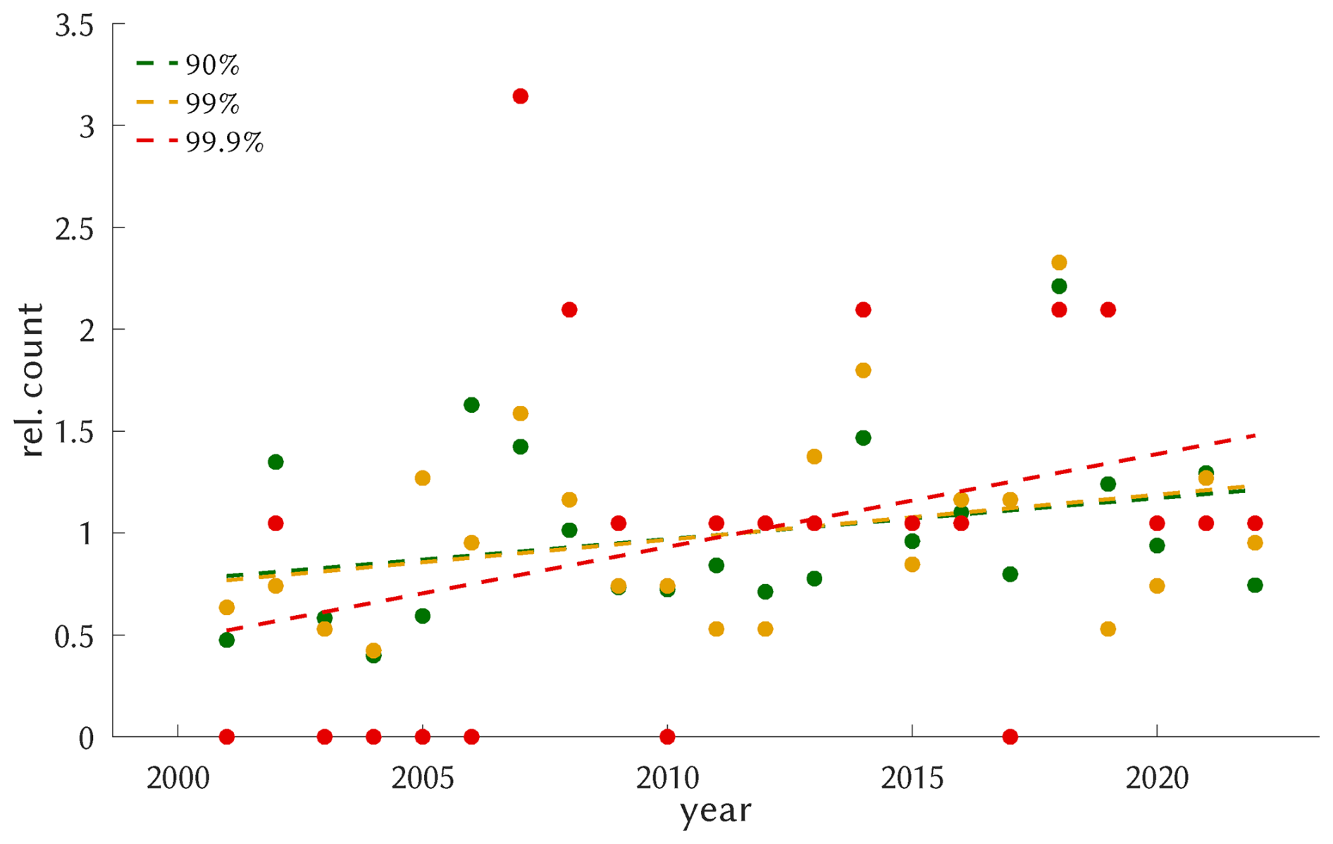
Figure 3For each percentile (90th, 99th, 99.9th), a single dot represents the annual exceedance count relative to the long-term average. The corresponding trends are positive but insignificant, indicated by the dashed linestyle.
One cannot get around the sample size limitation, however: as mentioned, only 208 cases remain when the analysis is limited to P99 and above (applied to all cases instead of annually); corresponding results should be interpreted with caution, hence. The sample size shrinks to 21 for P99.9 (and to 2 for P99.99).
3.1 Training and testing the classifiers with ERA5
The CatRaRE version used in this study covers the period from 2001 to 2022. By limiting the analysis to the summer months from May to August, a total of 10 824 6-hourly ERA5 fields remains to be classified according to the local conditions of CatRaRE. For the technical details of the probabilistic predictions, we refer to BH. The cases are split into a calibration (train) and validation (test) period of 2001–2011 and 2012–2022, respectively. For the DL training, cross-entropy loss (equivalent to logistic loss, see, e.g., Goodfellow et al., 2016) is used as a loss function, and the Ranked Probability Skill Score (RPSS) is used to assess the classification performance (RPSS is the skill score corresponding to the deviance of the predicted probabilities from the actual outcome, relative to predicting climatology; cf. Wilks, 2006, p. 302).
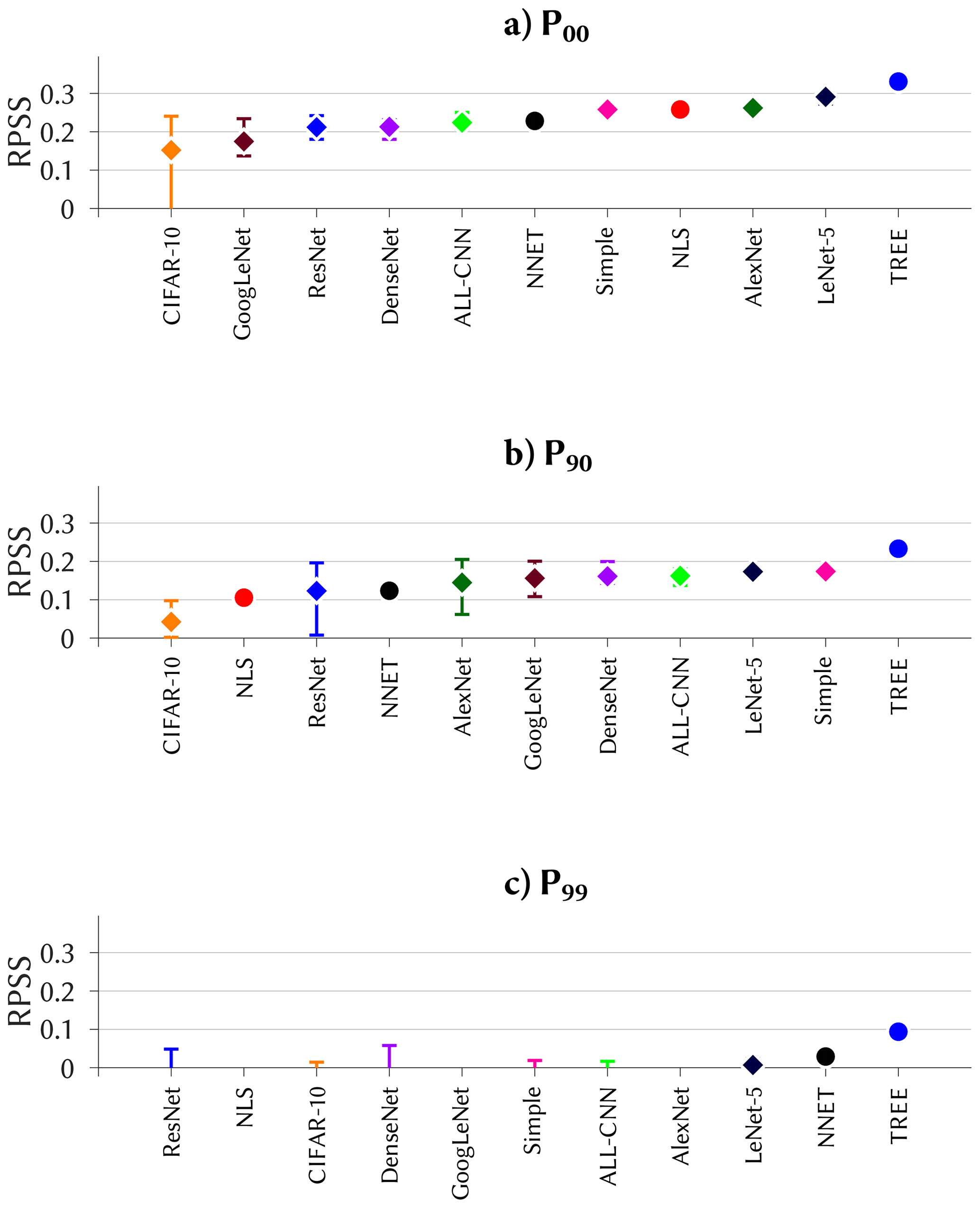
Figure 4Ranked probability skill score for the skillful classifiers, based on all CatRaRE events (a, P00) and on the upper extremes P90 and P99 (b, c). For visibility, classifiers with no skill (Logreg, LASSO) are skipped.
Figure 4 shows the scores for the respective severity classes P00, P90, and P99. For all, the TREE classifier outperforms all others markedly, including the DL methods, with scores of RPSS > 0.3 for P00 and RPSS > 0.2 for P90, in accordance to the findings of BH. The decreasing scores from P00 to P99, with the latter having almost no positive skill left, are in line with the decreasing sample size, or increasing rareness, of the classified events. This may have a number of reasons: very extreme events may not be represented as well in the ERA5 predictor fields; they may contain stronger stochastic elements; and as a simple arithmetic effect, misclassifications have a larger influence when numbers are small. We recall from BH that for DL there is a range in skill due to the stochastic nature of the optimization; for P90, some of the DL methods (ResNet, AlexNet, GoogLeNet) show a fairly large RPSS-range with maximum scores near that of TREE, but it is unclear how the stochastic nature of their training algorithm (Brownlee, 2018, cf.) can be “tricked” into finding that maximum every time. Compared to such highly sophisticated DL frameworks, the Simple DL with just one convolutional and one dense layer performs remarkably well, and that with almost no spread, even ranking second after TREE for the P90 case.
3.2 ERA5 and CMIP6 driving the trained classifiers
The trained classifiers are now applied to the observed (reanalyzed) and simulated atmospheric fields. The results are predicted probabilities for each of the 6 classes, cf. Sect. 2.3, at 6 h intervals from the respective summer months.
Our analysis starts by a case study in which we check whether the June 2001 event (see Fig. 2) is captured by our classification of the ERA5 fields. Figure 5 shows the probability forecasts from the TREE classifier for the cases P00 and P90. For both, a clear tendency is seen to generate elevated probabilities for non-zero classes towards mid-month. For P00, the SE and NW classes dominate at the start, the NE region is persistently prominent at mid-month, and the South again dominates in the decay phase. For P90, the evolution is much clearer: throughout the month of June there is essentially zero activity, to be interrupted only by three strong 6 h periods at mid-month, one occurring in NW and the other two in NE.
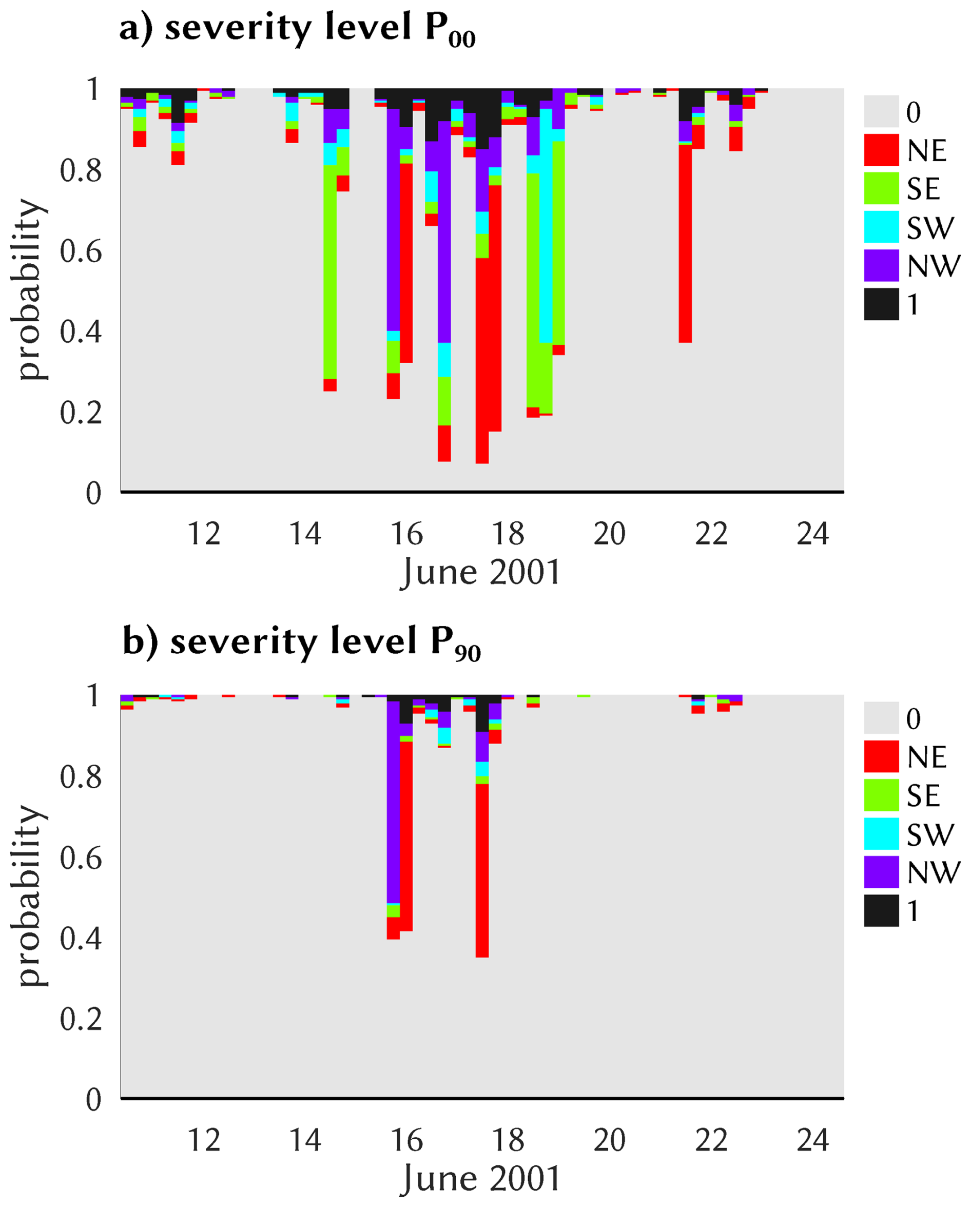
Figure 56-hourly probabilistic predictions of regional classes around the 17 June 2001 events, as obtained by the TREE classifier from ERA5 convective environments for the two severity levels P00 (a) and P90 (b).
To allow for a view at longer time scales, we form annual (i. e. May–August) averages of the resulting 6-hourly probabilities as obtained from the classifiers, and from now on focus entirely on these annual values and their centennial trends. We start by showing in Fig. 6 the results for the TREE classifier for class 1 and the entire ERA5 period 1979–2022; the other classifiers and regions are similar, cf. Figs. S1–S4 in the Supplement. The simulations quite well reproduce the observed base rate of class 1 for all severities P00, P90, and P99 of CatRaRE (cf. Table 2); interannual variability appears somewhat reduced. The ERA5-based trends are significantly positive throughout, with values of 3.1, 1.1, and 0.1 percentage points per century for the three severities, respectively. The simulated annual values are strongly correlated with observations for P00 and P90 (ρ=0.67 and ρ=0.43 for the validation period, resp.); such levels of correlation are somewhat surprising given the relatively poor sub-daily performance (cf. Fig. 4), but it adds confidence to using annual trends as the main target quantity. For P99, the performance is not easy to judge since, for example, observations have virtually no variability after 2015.
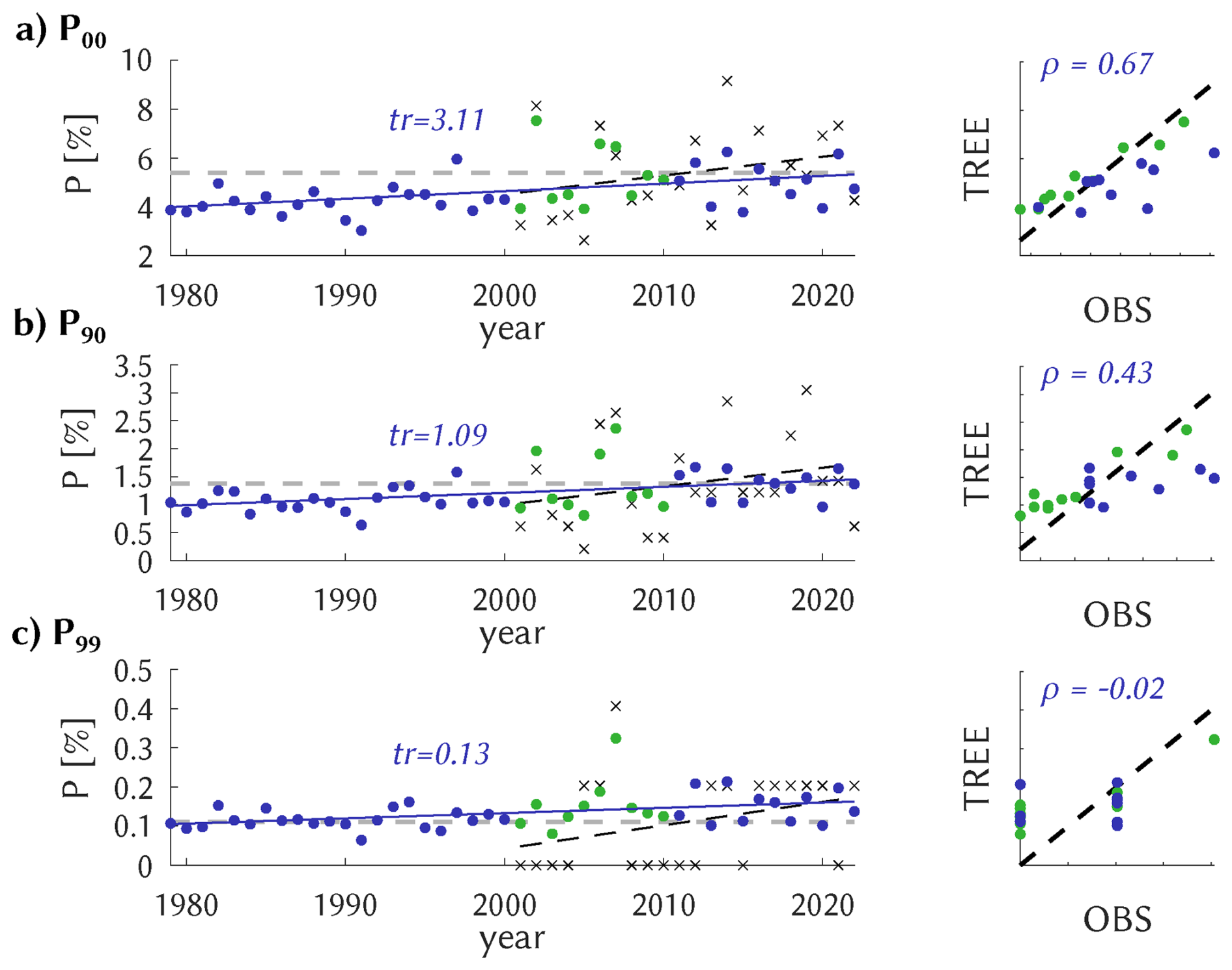
Figure 6Left: annual mean probabilities of class 1 occurrence for P00 (a), P90 (b), and P99 (c) from observations (CatRaRE class 1 relative frequency, black crosses) and from ERA5 using the TREE classifier as a time series (colored dots). Also shown is the centennial trend (solid if significant at 5 %). Right: the same as a scatter plot for the common period (2001–2022). The calibration period is indicated as green.
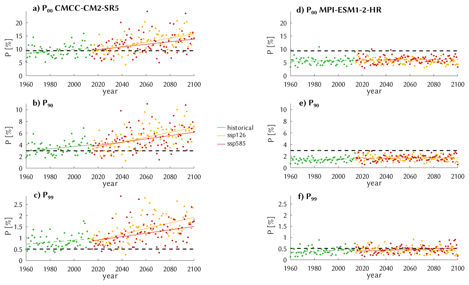
Figure 7Simulated annual probabilities of the 3 severity classes P00 (a, d), P90 (b, e), and P99 (c, f) occurring in the SW and corresponding centennial trends (solid if significant at 5 %), by applying the TREE classifier to the scenarios HIST (green), SSP126 (orange), and SSP585 (red) of the two GCMs CMCC-CM2-SR5 (a–c) and MPI-ESM1-2-HR (d–f). Also shown is the observational base rate as obtained for the period 2001–2022 (black dashed).
Now we turn to the simulated atmospheres as provided by the CMIP6 ensemble of climate simulations of Table 1. Given the 20 entries of the table (r1, r2, …), the 3 severity classes, the 6 regions, and the 12 classifiers, we have a total of centennial trends. For the illustration of individual results we confine ourselves to a few typical outcomes here and several more in the Supplement. The trend distribution is analyzed by discarding zero-skill classifiers and the two non-regional classes 0 and 1, leaving a total of 2400 regional trends. In Sect. 3.3 that distribution is subject to an ANOVA to disentangle the relevant sources of uncertainty. We start by showing in Fig. 7, similar to Fig. 6 for ERA5, examples for the SW region from two different GCMs. The TREE classifier is applied here to the climate scenarios HIST, SSP126, and SSP585 as simulated by CMCC-CM2-SR5 and by MPI-ESM1-2-HR. For the former, the simulations appear consistent with the overall observed base rate for the P00 and P90 case, the P99 case is positively biased. Compared to ERA5, cf. Fig. S4, interannual variability is increased. Furthermore, all trend lines point upward, most of them significantly. It is, however, noticeable – but possibly insignificant – that the warmest scenario SSP585 exhibits a weaker trend than the moderately warming SSP126. At first sight that may not seem to be in line with the narrative of warmer atmospheres generating heavier rainfall (e.g. Fowler et al., 2021), and we shall return to this point shortly. The results for the MPI-ESM1-2-HR model are less conclusive. Except for the extreme severity class P99 the values are negatively biased against observations, and no scenario exhibits a significant centennial trend. We have not been able to sort out any reason for this model behavior. Indeed, trend significance is more the exception than the rule, as of the 2400 cases only 610 are significant. Examples analogous to Fig. 7 are Figs. S5–S8.
Returning to the CMCC-CM2-SR5-based trends and their consistency with the global warming narrative, we inspect atmospheric drivers, cape, cin, and cp. To study their long-term behavior, we again form annual averages and corresponding trends, assuming implicitly that diurnal effects between them, such as cape depletion from convective precipitation, remain unaffected by climate change. Indeed, Fig. 8 may seem to violate that narrative, as model-simulated convective precipitation (cp) increases in the moderate SSP126 scenario but decreases in the warmer SSP585. But one also notes that while for cape those two future trends (which are both significantly positive) are not substantially different, the cin trend is markedly stronger for SSP585 and appears to dominate the negative influence on cp. It means that rainfall intensity indeed increases due to the stronger cape, but at the same time that rainfall frequency decreases due to the stronger cin, a delicate balance that can lead to a positive or a negative effect on rainfall amount depending on GCM, region, etc. Growing precipitation intensity is in line with the law of Clausius-Clapeyron and the global warming narrative; cin trends appear to depend on more factors, such as land vs. ocean, see Chen et al. (2020), Myhre et al. (2019), and also Sect. S3 of the Supplement. For the MPI-ESM1-2-HR model, corresponding trends are much weaker, and so is the negative influence of cin, leading to less divergence between the scenarios. More examples are presented in Figs. S9–S12.
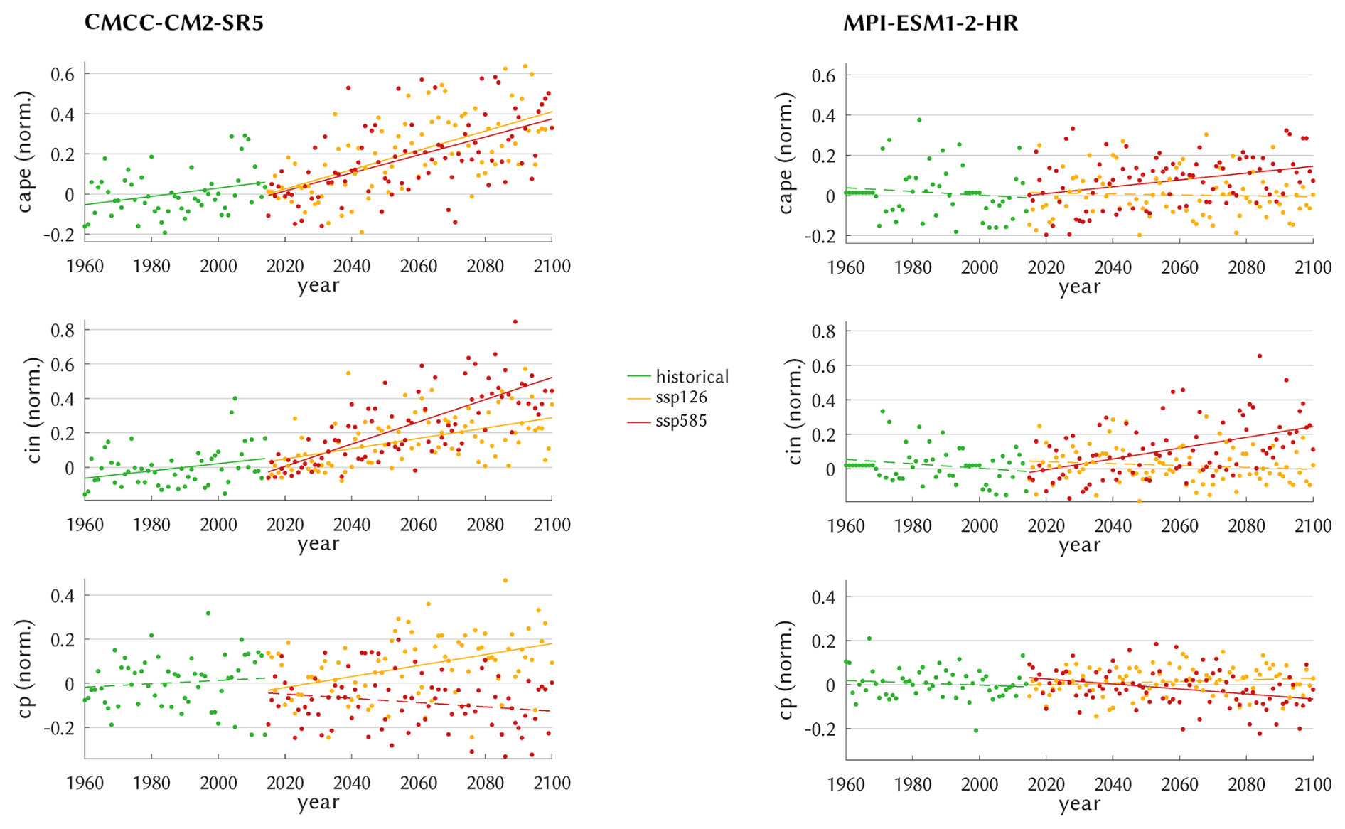
The above results pertain to the SW region. For the other regions no essential differences were obtained, which also reflects the results of the last section.
3.3 Distribution and ANOVA of the simulated trends
The distribution of the simulated trends is now investigated in the next figures. We start by showing in Fig. 9 the case of the classes with no regional focus, 0 (no events) and 1 (events anywhere), for the severity level P90. Despite a considerable range of uncertainty in all scenarios the majority 0-class decreases and the 1-class increases. The corresponding medians of the 0-class vary between −5 percentage points (for ERA5) and slightly below 0 percentage points (for SSP126). With a much smaller base rate the absolute class 1 trends are smaller as well, with a largest median from ERA5 just below 1 percentage points, a value that appears quite strong given a base rate of just 1.4 %, cf. Table 2; the GCM-based trends are smaller with medians varying near 0.2. The SSP585 trends for the 0-class (1-class) are generally more negative (positive) than the SSP126 trends, as would be expected from greenhouse forcing. The strong skewness for SSP126 may be related to the cape vs. cin antagonism that was potentially influential for the larger CMCC-CM2-SR5 amplitudes. The results for P00 are generally similar but with weaker amplitudes, cf. Fig. S13. Likewise, by confining to significant trends the overall picture does not change much, merely the strength of the trends is stronger and more in line with ERA5, cf. Fig. S14.
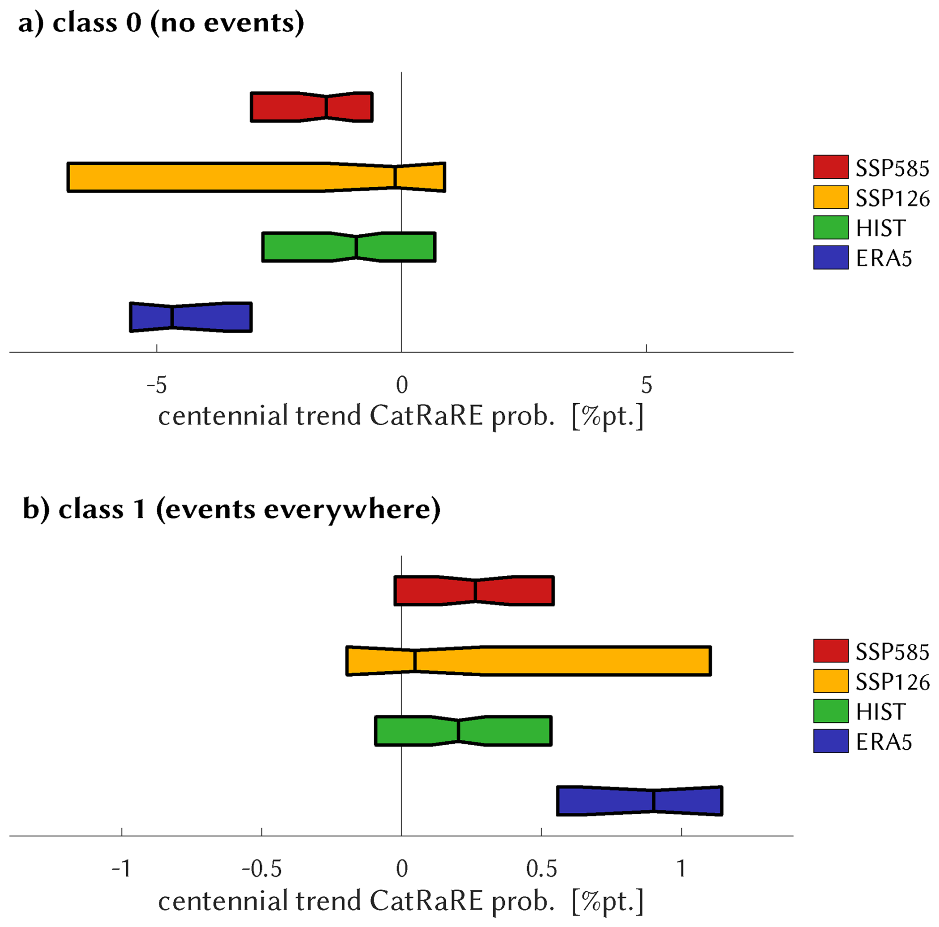
Figure 9For ERA5 and the HIST, SSP126, and SSP585 scenarios, boxplots of the distribution of centennial trends of simulated annual CatRaRE-type probabilities of severity type P90, for class 0 (a) and class 1 (b). Trend magnitude is given in percentage points. The width is determined by the inter-quartile-range and the vertical line depicts the median of the distribution. The different scaling of the x-axis is due to the much larger base rate of no events.
For the 4 quadrant regions, we depict trends relative to the respective base rate, to allow for a “fair” regional comparison. The overall message, shown in Fig. 10, is thus: trend uncertainty is large and the medians are positive throughout but below ERA5, whose medians vary regionally about half of the base rate. And contrary to the example of Fig. 7, for all regions the SSP585 median is larger than that of SSP126 (consistent with Fig. 9), and HIST is between both. For P00, see Fig. S15.
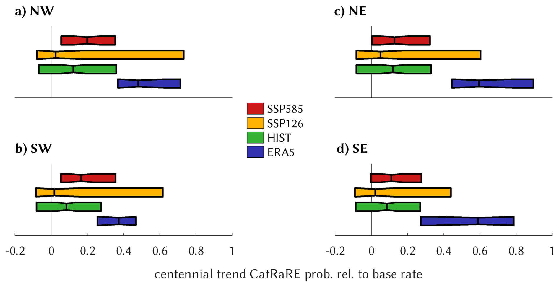
Figure 10Similar to Fig. 9, for the 4 quadrant regions. Trend magnitude is given relative to the respective base rate.
Each single trend is the result of a cascading set of model applications and assumptions, called “factors” here, and their entirety can to some degree be disentangled back into the single factors by employing the statistical machinery of ANOVA (= ANalysis Of VAriance). For the GCM-based simulations (HIST, SSP126, SSP585), the obvious factors are severity (SEV), scenario (SCN), climate model (GCM), classifier (DSC), and region (RGN); we do not consider factor interactions. One has to observe that including all trends would put too much weight on the RGN class because of the mostly negative trends of the 0-class vs. the positive trends for the others. To have comparable RGN classes we confine the ANOVA to the four quadrant classes NW, NE, SE, SW. We are thus left with the above mentioned total of 2400 trends, of which 610 are significant. Figure 11 shows the outcome in terms of the F-ratios of the factors, a measure that expresses the between-sample variance (factor effect) relative to the within-sample variance (background noise). For the case of all trends, by far the greatest influence on the centennial trends comes from the GCM factor, followed by SCN; DSC and RGN are very small, which for DSC is astonishing given the great diversity of classifiers. It means that most of the uncertainty is caused by the choice of GCM, even more than picking different emission scenarios. When confining the ANOVA to significant trends, the GCM F-ratio is largely reduced, and SCN remains the sole dominating factor. In other words, the significant trends are driven mainly by the scenarios.
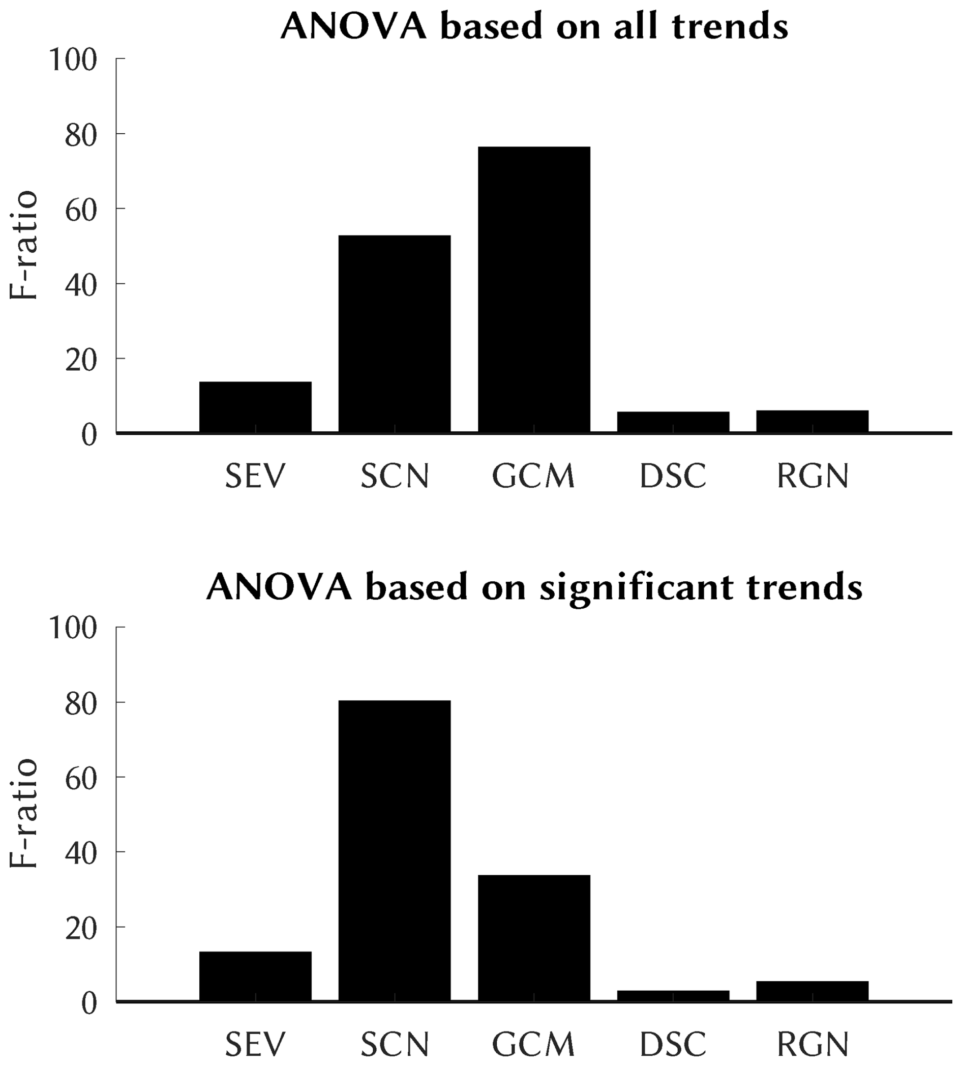
Figure 11Upper panel: F-ratio of ANOVA of the centennial trends for any of the four quadrant regions over the factors severity (SEV), climate scenarios (SCN), climate model (GCM), classifier downscaling (DSC), and region (RGN). All factors (i.e. its F-ratio) are significant. Lower panel: The same, confined to significant trends.
We have investigated past and future trends in the occurrence of extreme rainfall events. Our modeling chain consists of a CMIP6 ensemble of simulated atmospheric convective environments that are fed into statistical classifiers to predict occurrence probabilities of CatRaRE-type events over the four quadrant regions of Germany. The classifiers are trained on corresponding ERA5 fields, the learning target being the occurrence of CatRaRE events at a specified level of severity (all, upper 10 %, and upper 1 %). We are aware of, and have in the above analysis encountered, the trivial fact that increasing severity comes with a lower sample size and corresponding higher uncertainty. To counter this basic dilemma, we have employed an ensemble approach that tries to reflect as many aspects of the modeling chain as possible, and analyze the resulting distribution. We used as many of the current CMIP6 model data as we could retrieve (a number that is limited by the availability of upper tropospheric fields). As classifiers we have employed a wide range of conventional and more novel (“deep”) machine learning schemes. Based on the ranked probability skill score, various classification approaches were shown to be skillful when applied to ERA5, with the conventional tool of random forests outperforming all others; as is to be expected, towards the most rare and severe events the skill drops significantly. Of course, the approach to extreme rainfall trends can be widened to cover, for example, alternative concepts of extreme events itself (here CatRaRE) or their statistical estimation (here simple linear regression on annual quantiles). Before doing so one should, however, try to understand the large range of results that are already seen in the current setup, see below.
Regarding the convective environments we have found growing levels of both antagonistic drivers cape and cin, cf. Fig. 8. This is in line with current knowledge and has been attributed to the fact that rising greenhouse gases are causing, at lower levels, an increase in specific humidity and thus more latent heating and buoyancy, but over land a decrease in relative humidity and thus an elevated LFC, respectively (cf. Eqs. 1 and 2; Chen et al., 2020). The antagonism leads to higher uncertainty with respect to the future frequency of extreme convective events. But still, our analysis finds evidence that across Germany they are occurring more often, with only little differences between regions. This evidence, moreover, becomes clearer with growing levels of severity (Figs. 7, 9, 10), a fact that appears to be consistent with current observations, as exemplified by Fig. 1.
With respect to uncertainty in the centennial trends, the choice of classifier (downscaling) is less relevant, and so is the region considered. For downscaling this may be good news, as it means that very different approaches still arrive at similar results. The main source of uncertainty is the choice of climate model, followed by emission strength. This is reversed if insignificant trends are ignored, resulting in a largely reduced ensemble but with emissions now becoming the main factor for determining the trend.
The relevant code underlying this paper can be found at https://gitlab.dkrz.de/b324017/carlofff (last access: 11 November 2026) and is archived at Zenodo (https://doi.org/10.5281/zenodo.8146270, Bürger, 2023). Training and deployment of DL models is performed using the Caffe framework with its Octave interface (https://github.com/BVLC/caffe, Jia et al., 2014); using a corresponding container it can be run on various platforms.
All data are publicly available: CatRaRE at https://doi.org/10.5676/DWD/CatRaRE_W3_Eta_v2023.01 (Lengfeld et al., 2023), ERA5 at https://doi.org/10.24381/cds.adbb2d47 (Copernicus Climate Change Service, 2023), and CMIP6 data are available via the Earth System Grid at https://esgf.github.io/ (last access: 11 November 2026). Due to the diversity of modeling centers no unique DOI exists for CMIP6.
The supplement related to this article is available online at https://doi.org/10.5194/nhess-26-5897-2026-supplement.
GB and MH envisaged the project, GB developed and conducted the modeling, GB and MH wrote the manuscript.
The contact author has declared that neither of the authors has any competing interests.
Publisher's note: Copernicus Publications remains neutral with regard to jurisdictional claims made in the text, published maps, institutional affiliations, or any other geographical representation in this paper. The authors bear the ultimate responsibility for providing appropriate place names. Views expressed in the text are those of the authors and do not necessarily reflect the views of the publisher.
This research has been funded via the “ClimXtreme II” (sub-project CARLOFFF) by the German Ministry of Research, Technology and Space (Bundesministerium für Forschung, Technologie und Raumfahrt, BMFTR) in its strategy “Research for Sustainability” (FONA).
This research has been supported by the Bundesministerium für Bildung, Wissenschaft, Forschung und Technologie (grant no. 01LP2324B).
This paper was edited by Gregor C. Leckebusch and reviewed by two anonymous referees.
Bolton, D.: The computation of equivalent potential temperature, Mon. Weather Rev., 108, 1046–1053, 1980. a
Brownlee, J.: Statistical Methods for Machine Learning: Discover how to Transform Data into Knowledge with Python, Machine Learning Mastery, google-Books-ID: 386nDwAAQBAJ, https://machinelearningmastery.com/statistics_for_machine_learning/ (last access: 11 November 2026), 2018. a
Bürger, G.: Convective Atmospheres: Linking Radar-based Event Descriptors and Losses From Flash Floods (CARLOFFF), Zenodo [code], https://doi.org/10.5281/zenodo.8146270, 2023. a
Bürger, G. and Heistermann, M.: Shallow and deep learning of extreme rainfall events from convective atmospheres, Nat. Hazards Earth Syst. Sci., 23, 3065–3077, https://doi.org/10.5194/nhess-23-3065-2023, 2023. a
Bürger, G., Pfister, A., and Bronstert, A.: Temperature-driven rise in extreme sub-hourly rainfall, J. Climate, 32, 7597–7609, 2019. a
Chen, J., Dai, A., Zhang, Y., and Rasmussen, K. L.: Changes in Convective Available Potential Energy and Convective Inhibition under Global Warming, J. Climate, 33, 2025–2050, https://doi.org/10.1175/JCLI-D-19-0461.1, 2020. a, b
Copernicus Climate Change Service: ERA5 hourly data on single levels from 1940 to present, Copernicus Climate Change Service (C3S) Climate Data Store (CDS) [data set], https://doi.org/10.24381/cds.adbb2d47, 2023. a
Devadarshini, E., Geethalakshmi, V., McDermid, S. P., Bhuvaneswari, K., Mohan Kumar, S., Sathyamoorthy, N. K., Senthilnathan, S., Senthilraja, K., and Anandhi, V.: A systematic review of climate downscaling and extremes in Coupled Model Intercomparison Project 6 (CMIP6), Environmental Development, 56, 101280, https://doi.org/10.1016/j.envdev.2025.101280, 2025. a
Emmenegger, T., Ahmed, F., Kuo, Y.-H., Xie, S., Zhang, C., Tao, C., and Neelin, J. D.: The Physics behind Precipitation Onset Bias in CMIP6 Models: The Pseudo-Entrainment Diagnostic and Trade-Offs between Lapse Rate and Humidity, J. Climate, 37, 2013–2033, https://doi.org/10.1175/JCLI-D-23-0227.1, 2024. a
Fosser, G., Kendon, E. J., Stephenson, D., and Tucker, S.: Convection-Permitting Models Offer Promise of More Certain Extreme Rainfall Projections, Geophys. Res. Lett., 47, e2020GL088151, https://doi.org/10.1029/2020GL088151, 2020. a
Fowler, H. J., Lenderink, G., Prein, A. F., Westra, S., Allan, R. P., Ban, N., Barbero, R., Berg, P., Blenkinsop, S., Do, H. X., Guerreiro, S., Haerter, J. O., Kendon, E. J., Lewis, E., Schaer, C., Sharma, A., Villarini, G., Wasko, C., and Zhang, X.: Anthropogenic intensification of short-duration rainfall extremes, Nat. Rev. Earth Environ., 2, 107–122, https://doi.org/10.1038/s43017-020-00128-6, 2021. a, b
Gentine, P., Pritchard, M., Rasp, S., Reinaudi, G., and Yacalis, G.: Could Machine Learning Break the Convection Parameterization Deadlock?, Geophys. Res. Lett., 45, 5742–5751, https://doi.org/10.1029/2018GL078202, 2018. a
Goodfellow, I., Bengio, Y., and Courville, A.: Deep Learning, MIT Press, http://www.deeplearningbook.org (last access: 11 November 2026), 2016. a
He, K., Zhang, X., Ren, S., and Sun, J.: Deep Residual Learning for Image Recognition, in: 2016 IEEE Conference on Computer Vision and Pattern Recognition (CVPR), 770–778, https://doi.org/10.1109/CVPR.2016.90, 2016. a
Hersbach, H., Bell, B., Berrisford, P., Hirahara, S., Horányi, A., Muñoz-Sabater, J., Nicolas, J., Peubey, C., Radu, R., Schepers, D., Simmons, A., Soci, C., Abdalla, S., Abellan, X., Balsamo, G., Bechtold, P., Biavati, G., Bidlot, J., Bonavita, M., De Chiara, G., Dahlgren, P., Dee, D., Diamantakis, M., Dragani, R., Flemming, J., Forbes, R., Fuentes, M., Geer, A., Haimberger, L., Healy, S., Hogan, R. J., Hólm, E., Janisková, M., Keeley, S., Laloyaux, P., Lopez, P., Lupu, C., Radnoti, G., de Rosnay, P., Rozum, I., Vamborg, F., Villaume, S., and Thépaut, J.-N.: The ERA5 global reanalysis, Q. J. Roy. Meteor. Soc., 146, 1999–2049, https://doi.org/10.1002/qj.3803, 2020. a
Huang, G., Liu, Z., Van Der Maaten, L., and Weinberger, K. Q.: Densely Connected Convolutional Networks, in: 2017 IEEE Conference on Computer Vision and Pattern Recognition (CVPR), 2261–2269, https://doi.org/10.1109/CVPR.2017.243, 2017. a
Jekabsons, G.: M5PrimeLab: M5'regression tree, model tree, and tree ensemble toolbox for Matlab/Octave, http://www.cs.rtu.lv/jekabsons/Files/M5PrimeLab.pdf (last access: 11 November 2026), 2016. a
Jia, Y., Shelhamer, E., Donahue, J., Karayev, S., Long, J., Girshick, R., Guadarrama, S., and Darrell, T.: Caffe: Convolutional Architecture for Fast Feature Embedding GitHub [code], https://github.com/BVLC/caffe, (last access: 1 April 2025), 2014. a
Kendon, E. J., Prein, A. F., Senior, C. A., and Stirling, A.: Challenges and outlook for convection-permitting climate modelling, Philos. T. Roy. Soc. A, 379, 20190547, https://doi.org/10.1098/rsta.2019.0547, 2021. a
Krizhevsky, A., Sutskever, I., and Hinton, G. E.: ImageNet classification with deep convolutional neural networks, Commun. ACM, 60, 84–90, https://doi.org/10.1145/3065386, 2017. a, b
LeCun, Y., Boser, B., Denker, J. S., Henderson, D., Howard, R. E., Hubbard, W., and Jackel, L. D.: Backpropagation Applied to Handwritten Zip Code Recognition, Neural Comput., 1, 541–551, https://doi.org/10.1162/neco.1989.1.4.541, 1989. a, b
Lengfeld, K., Walawender, E., Winterrath, T., and Becker, A.: CatRaRE: A Catalogue of radar-based heavy rainfall events in Germany derived from 20 years of data, Meteorol. Z., 469–487, https://doi.org/10.1127/metz/2021/1088, 2021. a
Lengfeld, K., Walawender, E., Winterrath, T., Weigl, E., and Becker, A.: Heavy precipitation events Version 2023.01 exceeding DWD warning level 3 for severe weather based on RADKLIM-RW Version 2017.002 Parameter and polygons of heavy precipitation events in Germany version v2023.01, Deutscher Wetterdienst [data set], 2023, https://doi.org/10.5676/DWD/CatRaRE_W3_Eta_v2023.01, 2023. a
Lin, J., Qian, T., Bechtold, P., Grell, G., Zhang, G. J., Zhu, P., Freitas, S. R., Barnes, H., and Han, J.: Atmospheric Convection, Atmos.-Ocean, 60, 422–476, https://doi.org/10.1080/07055900.2022.2082915, 2022. a
Lucas-Picher, P., Argüeso, D., Brisson, E., Tramblay, Y., Berg, P., Lemonsu, A., Kotlarski, S., and Caillaud, C.: Convection-permitting modeling with regional climate models: Latest developments and next steps, WIREs Climate Change, 12, e731, https://doi.org/10.1002/wcc.731, 2021. a
McIlhagga, W.: penalized: A MATLAB Toolbox for Fitting Generalized Linear Models with Penalties, J. Stat. Softw., 72, 1–21, https://doi.org/10.18637/jss.v072.i06, 2016. a
Meyer, J., Neuper, M., Mathias, L., Zehe, E., and Pfister, L.: Atmospheric conditions favouring extreme precipitation and flash floods in temperate regions of Europe, Hydrol. Earth Syst. Sci., 26, 6163–6183, https://doi.org/10.5194/hess-26-6163-2022, 2022. a
Müller, M. and Kaspar, M.: Event-adjusted evaluation of weather and climate extremes, Nat. Hazards Earth Syst. Sci., 14, 473–483, https://doi.org/10.5194/nhess-14-473-2014, 2014. a
Myhre, G., Alterskjær, K., Stjern, C. W., Hodnebrog, Ø., Marelle, L., Samset, B. H., Sillmann, J., Schaller, N., Fischer, E., Schulz, M., and Stohl, A.: Frequency of extreme precipitation increases extensively with event rareness under global warming, Sci. Rep., 9, 16063, https://doi.org/10.1038/s41598-019-52277-4, 2019. a, b
O'Gorman, P. A. and Dwyer, J. G.: Using Machine Learning to Parameterize Moist Convection: Potential for Modeling of Climate, Climate Change, and Extreme Events, J. Adv. Model. Earth Sy., 10, 2548–2563, https://doi.org/10.1029/2018MS001351, 2018. a
Springenberg, J. T., Dosovitskiy, A., Brox, T., and Riedmiller, M.: Striving for Simplicity: The All Convolutional Net, arXiv [preprint], https://doi.org/10.48550/arXiv.1412.6806, 2014. a
Szegedy, C., Liu, W., Jia, Y., Sermanet, P., Reed, S., Anguelov, D., Erhan, D., Vanhoucke, V., and Rabinovich, A.: Going deeper with convolutions, in: 2015 IEEE Conference on Computer Vision and Pattern Recognition (CVPR), 1–9, https://doi.org/10.1109/CVPR.2015.7298594, 2015. a
Taszarek, M., Allen, J. T., Marchio, M., and Brooks, H. E.: Global climatology and trends in convective environments from ERA5 and rawinsonde data, npj Clim. Atmos. Sci., 4, 1–11, https://doi.org/10.1038/s41612-021-00190-x, 2021. a
Trenczek, J., Lühr, O., Eiserbeck, L., Sandhövel, M., and Leuschner, V.: Übersicht vergangener Extremwetterschäden in Deutschland, Projektbericht “Kosten durch Klimawandelfolgen”. Methodik und Erstellung einer Schadensübersicht. Studie im Auftrag des Bundesministeriums für Wirtschaft und Klimaschutz, https://www.prognos.com/sites/default/files/2022-07/Prognos_KlimawandelfolgenDeutschland_%C3%9Cbersicht%20vergangener%20Extremwettersch%C3%A4den_AP2_1.pdf (last access: 11 November 2026), 2022. a
Ukkonen, P. and Mäkelä, A.: Evaluation of Machine Learning Classifiers for Predicting Deep Convection, J. Adv. Model. Earth Sy., 11, 1784–1802, https://doi.org/10.1029/2018MS001561, 2019. a
Wilks, D. S.: Statistical Methods in the Atmospheric Sciences, Academic Press, https://doi.org/10.1016/C2017-0-03921-6, 2006. a
Winterrath, T., Brendel, C., Hafer, M., Junghänel, T., Klameth, A., Lengfeld, K., Walawender, E., Weigl, E., and Becker, A.: Radar climatology (RADKLIM) version 2017.002; gridded precipitation data for Germany: Radar-based gauge-adjusted one-hour precipitation sum (RW), Deutscher Wetterdienst [data set], https://doi.org/10.5676/DWD/RADKLIM_RW_V2017.002, 2018. a