The operational 3DEnVar data assimilation scheme for the Météo-France convective scale model AROME-France

Since October 2024 the Météo-France operational convective scale model AROME-France has been using a 3DEnVar data assimilation (DA) scheme in order to improve the performance of severe weather prediction. This paper describes the configuration and evaluation of this 3DEnVar scheme. It summarizes the work carried out to configure this scheme in an operational context, with the inherent constraints of numerical robustness, compatible execution times, and of course correct performance of the forecasts produced. The adjustment of horizontal and vertical localization, inflation, hybridization, and the use of Incremental Analysis Updates (IAU) are studied in sensitivity experiments, and the impact on the spin-up is investigated. A configuration and its variation with IAU are thus defined and evaluated using different scores over a long period and on different severe meteorological situations (winter storms, fog, and High Precipitating Events): they largely outperform the operational 3D-Var. The version with IAU was implemented in the new operational version of the AROME-France assimilation system.

1 Introduction

For 15 years now, AROME-France has been the Météo-France operational Numerical Weather Prediction (NWP) System for convective scales. Since the beginning, this model, as many of its equivalents (Gustafsson et al., 2018), has been equipped with a Data Assimilation (DA) system that benefits from initial conditions that contain information at scales that the model resolves. Using the same principles as for lower resolution NWP systems, this DA system combines regional observations with a previous high resolution model forecast (the background) to produce a 3D analysis at the model resolution. The first version (Seity et al., 2011) used a 2.5 km horizontal resolution in a 3 h continuous assimilation cycle, based on a 3D-Var scheme. Numerous improvements to the AROME-France system have been implemented, then released into operations approximately once a year, of which two major ones occurred in April 2015 (Brousseau et al., 2016): the increase of vertical and horizontal model resolution and the increase of the DA cycle frequency (from a 3 to a 1 h period cycle).

This DA system has demonstrated its ability to provide very useful information to improve general scores of forecast performance. In many situations, it has also helped forecasters to take the right decisions during high impact events (High Precipitating Events, fog events, storms, etc.). However, it suffers from two major flaws:

• the use of climatological background error statistics (the so-called B matrix) modelled using the Berre (2000) formulation in spectral space under the assumption of horizontal homogeneity and isotropy (Brousseau et al., 2011),

• the lack of a temporal dimension within the assimilation window in the 3D scheme, which restricts the frequency of assimilated observations to the assimilation cycle frequency, as well as the temporal resolution of the comparison of the observation to the background. While the use of the First Guess at Appropriate Time (FGAT) approach may address the latter issue, it does not yield any improvements regarding the former (Brousseau, 2012).

Regarding the first limitation, numerous studies have tried to introduce some flow-dependent features into the AROME-France framework, using either an update of the different coefficients implied in the covariance formulation (Brousseau et al., 2012; El-Said et al., 2022) or geographical masks to deal with dependencies on different meteorological phenomena (Montmerle and Berre, 2010; Ménétrier and Montmerle, 2011). However, the impact on the performance remains very weak compared to the increase of the numerical cost of such implementations. Furthermore, larger improvements can be expected from ensemble-based formulations such as the 3DEnVar implemented at NCEP (Wu et al., 2017) and the Local Ensemble Transform Kalman Filter (LETKF) used in operations at DWD (Schraff et al., 2016). Concerning the second limitation, several NWP operational centers (UK Met Office, Ballard et al., 2016, Japan Meteorological Agency, Honda and Sawada, 2008) currently employ a 4D-Var scheme, using an analysis increment at a lower horizontal resolution than the non-linear model, in order to keep the numerical cost within acceptable limits for operational use (see also Gustafsson et al., 2012 for a previous regional 4D-Var application with analysis increments at 48 km resolution). A prototype of a 4D-Var scheme for AROME-France has already been tested. On one hand, the development of the tangent linear and adjoint versions of the non-linear model is very difficult in a convective scale system. On the other hand, the resulting improvement remains weak compared to the numerical cost increase.

At Météo-France, these two limitations are now addressed through the EnVar approach, which consists in specifying background error covariances directly from an ensemble of perturbed forecasts, provided by an ensemble of data assimilations (EDA) (Hamill and Snyder, 2000; Lorenc, 2003; Buehner, 2005). Such fully flow-dependent covariances are then used in a variational context to produce a deterministic analysis. Moreover, as demonstrated in numerous studies (Desroziers et al., 2014; Wang and Lei, 2014; Gustafsson and Bojarova, 2014), this approach makes it possible to derive temporal background error cross correlations, and thus to formulate a 4DEnVar cost function involving a 4D state (i.e. the succession of the different 3D model states along the assimilation window). In this context, the information of an observation at a given time is propagated to other instants of the 4D assimilation window by the 4D background error covariances in order to produce an analyzed 4D state. In this way, a 4D scheme can be implemented without developing the tangent linear and adjoint models for complex model components (e.g. micro-physics, non-hydrostatic dynamics). Furthermore, the numerical cost of this approach is lower than that of 4D-Var. The minimization process does not require any model integration and the numerical cost partly depends on the number of assimilation window timeslots. The main numerical cost increase is due to the computation of the newly required EDA and can be adjusted with the horizontal resolution or the size of the ensemble for example. The drawback of EnVar methods is the need for localization in order to remove long-range correlations in background error covariances affected by sampling noise due to a limited ensemble size.

The development of a 3DEnVar version presented in this study is a first step towards a 4DEnVar scheme for AROME-France, and a major component of the scientific forward planning of Météo-France's NWP activities. Such schemes facilitate a lot of further developments, such as the extension of the control vector to hydrometeors (Wang and Wang, 2017; Destouches et al., 2023), since background error covariances for these new variables are directly available from the EDA. Consequently, the direct assimilation of radar reflectivities or lightning observations (Combarnous et al., 2024) can be considered.

In this context, two early preparatory studies have already been published, regarding preliminary 3DEnVar experiments at Météo-France:

• Montmerle et al. (2018, MO18 hereafter) presented the formulation and some preliminary tests concerning a first 3dEnVar scheme for AROME-France.

• Michel and Brousseau (2021, MI21 hereafter) focused on a hybrid configuration, merging climatological and flow-dependent background error covariances of a dual-resolution 3DEnVar scheme.

As first results of both studies were promising, numerous investigations have been conducted since their publication in order to be able to use a 3DEnVar scheme in the operational AROME-France system, with the following objectives:

• to tune and implement a robust system in an operational context with its associated constraints: robustness, numerical cost and stability, temporal constraint for the operational use, etc.

• to outperform the 3D-Var scheme in terms of meteorological quality of the forecast provided to forecasters,

• to propose a system allowing further developments. This includes the use of the OOPS (Object-Oriented Prediction System) software framework, and if possible a configuration using the full (i.e. non-hybrid) ensemble background error covariance matrix. These would facilitate the shift towards 4DEnVar planned for the next evolution, or the extension of the control vector (the vector of variables explicitly modified by the DA scheme) to variables missing in the current modeling of the B matrix (e.g. hydrometeors, non hydrostatic variables, surface variables).

The present article aims at summarizing these investigations and describing the retained configuration and its performance. After the introduction, Sect. 2 introduces the 3DEnVar formulation, describes how this new data assimilation scheme is integrated into Météo-France's numerical weather prediction (NWP) system, and outlines the context and motivation for the present study. The third section is dedicated to sensitivity experiments performed to tune the system. The performance of the selected configuration compared to the previous 3D-Var scheme is evaluated using statistical scores in the fourth section. A focus on different severe meteorological events such as winter storms, fog and High Precipitating Events (HPEs) is made in Sect. 5 to complete a comprehensive evaluation of the new system.

2 Configuration setting

2.1 3D-Var and 3DEnVar formulations

MO18 and MI21 described the formulations used in both studies to minimize the following incremental 3D cost function J:

$$J\left(\mathit{\delta }\mathbf{x}\right)={\displaystyle \frac{\mathrm{1}}{\mathrm{2}}}\left(\mathit{\delta }\mathbf{x}{)}^T{\mathbf{B}}^{-\mathrm{1}}\right(\mathit{\delta }\mathbf{x})+{\displaystyle \frac{\mathrm{1}}{\mathrm{2}}}{\left(\mathbf{d}-\mathbf{H}\mathit{\delta }\mathbf{x}\right)}^T{\mathbf{R}}^{-\mathrm{1}}(\mathbf{d}-\mathbf{H}\mathit{\delta }\mathbf{x})$$

where δx stands for the analysis increment, the difference between the analysis and the background, B and R respectively represent the matrices of background and observation error covariances. d = y^o−ℋ(x^b) is the innovation vector representing the difference between the observations y^o and the background x^b projected in the observation space by the observation operator ℋ, H being the linearized version of the latter. This cost function is quadratic and nullifying its gradient leads to solving the following linear system:

$$\left({\mathbf{B}}^{-\mathrm{1}}+{\mathbf{H}}^T{\mathbf{R}}^{-\mathrm{1}}\mathbf{H}\right)\mathit{\delta }\mathbf{x}={\mathbf{H}}^T{\mathbf{R}}^{-\mathrm{1}}\mathbf{d}$$

which needs to be preconditioned for efficiency, through a change of variable. The square root form δx = ${\mathbf{B}}^{\mathrm{1}/\mathrm{2}}\mathcal{X}$, which can be solved with the conjugate gradient algorithm, is historically used at Météo-France.

The 3D-Var scheme involves a climatological parametrized background error matrix hereafter noted B_s. In the versions of AROME-France using a 3D-Var DA scheme, ${\mathbf{B}}_{\mathrm{s}}^{\mathrm{1}/\mathrm{2}}$ is modeled following the Berre (2000) multivariate formulation, which involves a sequence of linear operators to represent variances, correlations and cross-covariances between the different variables of the control vector. Brousseau et al. (2011) used an AROME-EDA at the model resolution to calibrate the different operators.

The 3DEnVar scheme, now implemented in AROME-France, is based on the use of a B matrix directly sampled from an AROME-EDA noted B_e:

$${\mathbf{B}}_{\mathrm{e}}=\mathbf{C}\circ {\mathbf{XX}}^T$$

where C is the localization matrix, “∘” the Schur product and X = $\left[{\mathit{ϵ}}_{\mathrm{1}},{\mathit{ϵ}}_{\mathrm{2}},\mathrm{\dots },{\mathit{ϵ}}_{n_{\mathrm{e}}}\right]$, the perturbation matrix in which every column contains the deviation ϵ_l = $\frac{\mathrm{1}}{\sqrt{n_{\mathrm{e}}-\mathrm{1}}}\left({\mathbf{x}}_l^{\mathrm{ae}}-{\stackrel{\mathrm{‾}}{\mathbf{x}}}^{\mathrm{ae}}\right)$ of an ensemble member model state ${\mathbf{x}}_l^{\mathrm{ae}}$ with respect to the ensemble mean ${\stackrel{\mathrm{‾}}{\mathbf{x}}}^{\mathrm{ae}}$ (where n_e is the ensemble size and superscript ae stands for AROME-EDA state interpolated onto the 1.3 km horizontal AROME-France grid).

Finally, a hybrid scheme used in MI21 merges these two approaches with B = ${\mathit{\beta }}_{\mathrm{s}}^{\mathrm{2}}{\mathbf{B}}_{\mathrm{s}}+{\mathit{\beta }}_{\mathrm{e}}^{\mathrm{2}}{\mathbf{B}}_{\mathrm{e}}$ where ${\mathit{\beta }}_{\mathrm{s}}^{\mathrm{2}}$ and ${\mathit{\beta }}_{\mathrm{e}}^{\mathrm{2}}$ are scalar weights.

2.2 Météo-France operational numerical weather prediction system and data flow

The Météo-France numerical weather prediction system used in operations contains two main models and their different versions (Fig. 1):

• the global model ARPEGE (Courtier et al., 1994; Bouyssel et al., 2021) that uses a stretched grid with a horizontal resolution of 5 km over France. It employs a multi-incremental 4D-Var scheme (2 outer-loops) in a 6 h data assimilation cycle. Background errors are simulated by running a 50-member ARPEGE-EDA (Fisher, 2003; Raynaud et al., 2011), allowing flow-dependent covariances to be specified. Since October 2024, the B matrix is a hybrid combination (Berre and Arbogast, 2024) of covariances localized in gridpoint space and of covariances modeled in wavelet space (Berre et al., 2015), which are both computed from the ARPEGE-EDA.

• the limited area model AROME-France (Seity et al., 2011) at 1.3 km using a 3DEnVar scheme (instead of the historical 3D-Var that was used before October 2024) in a hourly cycle (Brousseau et al., 2016). An AROME-EDA is run at the lower horizontal resolution of 3.2 km (MI21) in a 3 h cycle in order to reduce the numerical cost of the 50 members currently used.

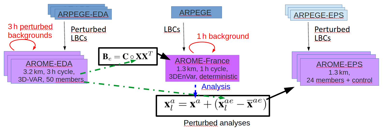
Figure 1 Schematic representation of the data exchanges between the main components of the Météo-France NWP operational system (deterministic, EDA and EPS versions) for the global model ARPEGE (blue rectangles) and the LAM AROME-France (purple rectangles). B_e is the ensemble background error covariance matrix, C the localization matrix, “∘” the Schur product and X the perturbation matrix provided by the AROME-EDA. x is a model state, $\stackrel{\mathrm{‾}}{\mathbf{x}}$ the ensemble mean. Subscript l stands for an ensemble member and superscript a (resp. ae) for analysis (resp. AROME-EDA model state interpolated on the 1.3 km AROME-France horizontal grid).

One can note that these two main systems are complemented by their Ensemble Prediction System (EPS) versions, ARPEGE-EPS (Descamps et al., 2015) over the globe and AROME-EPS (Raynaud and Bouttier, 2017) for the limited area version. Both EPS systems run at the same horizontal resolution as their deterministic equivalents since the operational upgrade of June 2022. They consist of 35 and 24 members respectively. The uncertainties of their initial conditions are sampled from their respective EDAs. For AROME-EPS, 24 perturbed initial atmospheric conditions are obtained by starting from the AROME-France deterministic analysis (x^a) and adding 24 random draws among the 50 available differences $({\mathbf{x}}_l^{\mathrm{ae}}-{\stackrel{\mathrm{‾}}{\mathbf{x}}}^{\mathrm{ae}})$ from the AROME-EDA (Fig. 1). Other AROME configurations (not represented in Fig. 1) also exist for nowcasting purposes (Auger et al., 2015) and overseas domains (Faure et al., 2020), without assimilation for the latter. The reader can refer to the respective references for more details. Only the AROME-France data assimilation system and its EDA version (AROME-EDA) are detailed here.

AROME-France uses the 3DEnVar scheme described in this paper in a 1 h cycle. AROME-EDA still relies on the 3D-Var scheme (Fischer et al., 2005) in a 3 h cycle. Both assimilate a wide range of observation types, including radar reflectivities through retrievals of humidity profiles (Caumont et al., 2010; Wattrelot et al., 2014), radial winds from Doppler weather radars over Europe (Montmerle and Faccani, 2009; Martet et al., 2022), brightness temperatures from various instruments on polar orbiting and geostationary satellites (Guidard et al., 2011) as well as ground-based GNSS atmospheric path delays (Mahfouf et al., 2015) in addition to conventional observations.

Data exchanges between the different systems are illustrated in Fig. 2. This figure specifically shows all the exchanges required to run the DA cycle of AROME-France at 11:00, 12:00, and 13:00 UTC, as well as the extended (“long”) forecasts at 12:00 UTC. It also depicts the sequence in which the various systems are executed and the resulting coupling choices. This execution pattern repeats throughout the day. More precisely, the 1 h range forecasts of the DA cycle (plain red arrows) asynchronously use Lateral Boundary Conditions (LBCs) from the latest available ARPEGE forecast. For example executions at 08:00, 09:00, 10:00, 11:00, 12:00 and 13:00 UTC analysis times use LBCs from the 06:00 UTC ARPEGE analysis time (dotted black arrows). On the contrary, long forecasts used in operations are launched 8 times a day (every 3 h, for example at 09:00 and 12:00 UTC in Fig. 2) and use synchronous LBCs from ARPEGE to benefit from the most recent LBCs, with a positive impact on the performance. These long forecasts also have the particularity in that they are initialized with the AROME analysis valid at H but are also updated by Incremental Analysis Update (IAU; Bloom et al., 1996) of the H+1 analysis (dashed blue arrows in Fig. 2) to benefit from the most recent observations available when this forecast is effectively launched (Brousseau et al., 2016). This particular setup implies that the H+1 analysis has to be executed just after the H one. The reader can note that, in this configuration, the IAU is not used for its filtering properties, but is employed to update the forecast with more recently observed information.

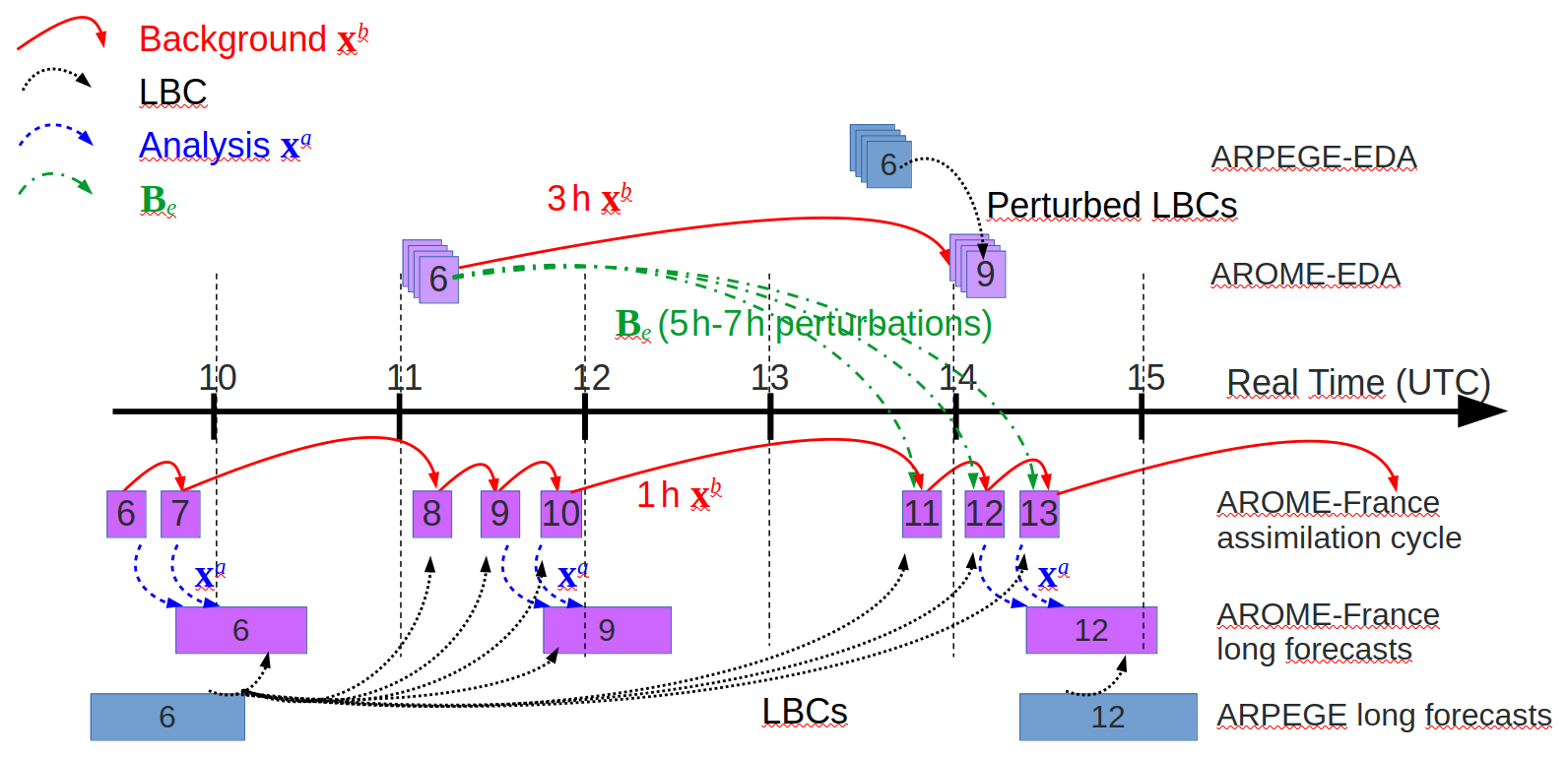
Figure 2 Temporal implementation of the operational AROME-France model from the 08:00 to the 13:00 UTC analysis times (with the same pattern repeated throughout the day for other analysis times). The rectangles represent the execution of an assimilation-forecast block, each corresponding to the analysis time indicated by the number within the rectangle. These blocks are positioned along the time axis according to their actual execution time. The length of each rectangle is proportional to the wall-clock time required to complete the block on Météo-France's high-performance computing (HPC) system. Purple rectangles denote AROME runs, blue rectangles denote ARPEGE runs, and stacked rectangles represent ensemble systems. Here, x refers to a model state, with the superscript a (respectively b) indicating the analysis (respectively, the background state).

The operational AROME-EDA aims to simulate the propagation of different errors through the assimilation cycle in order to sample initial uncertainties in the operational AROME-EPS (Raynaud and Bouttier, 2016), and to provide background error covariances to the EnVar schemes. Model errors are taken into account by perturbing the total parametrized tendencies of physical processes with multiplicative noise (SPPT: Buizza et al., 1999) implemented in the AROME-EPS by Bouttier et al. (2012). Observation errors are simulated by adding random draws from the observation error covariance matrix. The addition of such model and observation perturbations and their propagation in the assimilation cycle allows analysis and background errors to be simulated (Brousseau et al., 2011). Finally, the LBC errors are represented through the use of perturbed LBCs asynchronously provided every 6 h by the global ARPEGE-EDA given by the availability of the different forecasts in real time: H and H-3 AROME-EDA assimilation times (where H is either 00:00, 06:00, 12:00 or 18:00 UTC) use LBCs from the H-6 ARPEGE-EDA assimilation time.

Regarding this organization and the way the different systems are linked and strongly dependent on each other, the AROME-France 3DEnVar analyses have to use perturbations from the AROME-EDA in an asynchronous way.

For example, the AROME-France analyses at 11:00, 12:00, and 13:00 UTC respectively use 5, 6, and 7 h range perturbation matrices X (dashed-dotted green arrows) from the 06:00 UTC AROME-EDA analysis time to estimate B_e.

2.3 Software framework

AROME-France was historically developed using the same code base as ARPEGE and IFS, as part of a collaboration between ECMWF, Météo-France and its LAM partners from the ALADIN and HIRLAM consortia (now merged into the ACCORD consortium). The Object-Oriented Prediction System (OOPS) project began in 2009 with the aim of upgrading the shared data assimilation code to facilitate the development of new algorithms and simplify maintenance. It uses an object-oriented design and consists in adding an upper-level C++ code layer to the existing IFS-ARPEGE-LAM FORTRAN code, which required significant refactoring of the latter. The majority of the coding work has now been completed. While previous versions of the code included prototypes for initial investigations and developments, the cy48 version is fully operational and enables the execution of AROME and ARPEGE DA systems with all the features present in the original FORTRAN code, including all operational observation types, variational bias correction and digital filters. In addition, OOPS enables the use of various data assimilation (DA) schemes (3D-Var, 3DEnVar, 4DEnVar, hybrid versions, etc.), of different minimizers or preconditioning, and allows the control vector to be easily modified (e.g. variables can be added or changed). All the experiments used in this study were performed using OOPS (including the 3D-Var reference experiment), using the cy46 version for earlier runs and the cy48 version for later ones.

2.4 Summary of previous studies

As stated in the introduction, two early preparatory studies regarding preliminary 3DEnVar experiments at Météo-France have already been published:

• MO18 (Montmerle et al., 2018) presented the formulation and some preliminary tests concerning the localization, hybrid formulation and DA experiment. Results were promising as the 3DEnVar scheme outperformed standard 3D-Var in an experimental study conducted over a 5-week winter period. This study had the advantage of being performed using a prototype of OOPS, which was due to replace the historical framework in ARPEGE/AROME/IFS. Nevertheless, it used a non operational configuration with a 3.8 km horizontal resolution, both for the ensemble and the deterministic model (versus 1.3 km in operations for the latter) and a 3 h period DA cycle (versus 1 h in operations).

• MI21 (Michel and Brousseau, 2021) evaluated a dual-resolution 3DEnVar scheme (1.3 km for the deterministic model, 3.2 km for the EDA) in an hourly cycle as in the operational system. A hybrid configuration, merging climatological and flow-dependent background error covariances, was tuned and evaluated over a 3-month summer period, confirming better performance of hybrid 3DEnVar compared to 3D-Var. Numerous sensitivity studies related to localization lengths, ensemble size or hybrid weights have also been done. However, this study presents two weaknesses. Firstly, the use of the historical ARPEGE/AROME/IFS software framework makes further developments technically much more cumbersome than with OOPS. Likewise, the exclusive use of a hybrid formulation makes some scientific developments much more complex, as the temporal dimension (4DEnVar) or the covariances involving the new variables (hydrometeors) are not fully managed with the hybrid B matrix, whereas they are in a fully ensemble-based one.

Regarding these two articles, the following settings have been selected as a basis for the investigations described in the present study. The 3DEnVar scheme uses the ${\mathbf{B}}^{\mathrm{1}/\mathrm{2}}$ preconditioning and the associated cost function as in MI21. The localization is done in spectral space as in MO18, without using any recursive filter as in MI21, mainly as a preliminary step towards the use of the Scale Dependent Localization (SDL; Caron et al., 2019). The same localization is applied to all variables in order to be factorized and applied only once, allowing the numerical cost to be reduced. The control vector includes temperature (T), surface pressure (P_s), specific humidity (q) and the two horizontal wind components (u and v), instead of vorticity and divergence, in order to use similar spatial scales when applying this common localization length scale (Berre et al., 2017). Ménétrier et al. (2015) have proposed a theory that allows the diagnosis of optimal localization length scales using only information from the ensemble. MO18 used this method to estimate a common localization length scale in the AROME EDA framework; in the AROME-France 3DEnVar they retained and evaluated a value of 170 km, constant in the vertical, despite a diagnosed vertical profile increasing with altitude. MI21 obtained better performance by reducing this constant value to 40 km. The important choice of the localization length scales is thus discussed in the following section, in addition to other features such as the potential use of a hybrid version, a coefficient of inflation to adjust the ensemble spread, or the use of an IAU technique to reduce the spin-up.

3 Tuning of the 3DEnVar scheme

3.1 Methodology

The first goal of these investigations is to build a data assimilation cycle allowing subsequent forecasts to perform better than if it were 3D-Var. In order to have consistent results, all sensitivity tests will be compared using the diagnostics that have been found to be representative of the obtained results. Two kinds of diagnostics have been selected. The first one is the Root Mean Square (RMS) of observation-guess (O-B) and observation-analysis (O-A) differences in observation space for several observation types. We focused here on observations with a wide spatial and temporal coverage over the AROME-France geographical domain: aircraft measurements of temperature and wind from commercial airlines that are informative on the larger scales, and radar reflectivities that are informative on the smaller scales resolved by the system, and which are more representative of convective scale phenomena. Relative differences of RMS of O-A and O-B between the different experiments are summarized in Fig. 3.

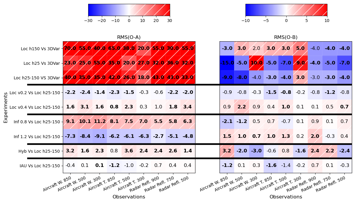
Figure 3 Relative difference (%) of RMS(O-A) (left panel) and RMS(O-B) (right panel) between different pairs of experiments (labeled on the left side of each line) for aircraft Wind, aircraft Temperature and radar reflectivity measurements at different atmospheric levels (hPa). Positive (resp. negative) difference values in red (resp. in blue) indicate larger (resp. smaller) RMS values in the experiment (first part of the left label) compared to the reference (second part of the left label). Bold numbers indicate statistically significant differences using a student test with a 95 % confidence interval.

The second diagnostic is the precipitation scores resulting from the comparison between (i) 24 h accumulated precipitation observed by a blend of radar and rain-gauge measurements from the ANTILOPE product (Laurantin, 2013) and (ii) 24 h accumulated precipitation simulated by the sum of the 1 h precipitation accumulation from the successive 1 h forecasts of the DA cycle over 24 h. Since the simulated precipitation can be seen as the result of a temporal and vertical integration of the different prognostic fields of the model, this diagnostic appears to be a good measurement of the general behavior of the system. Relative differences of Heidke Skill Score (HSS) for 24 h accumulated precipitation are presented in Fig. 4.

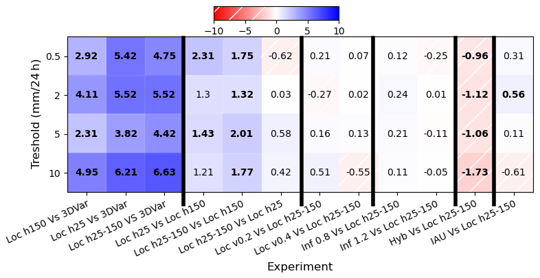
Figure 4 Relative difference (%) of HSS between different pairs of experiments (labeled at the bottom of each column). For each experiment comparison, the HSS relative difference for the 0.5, 2, 5 and 10 mm 24 h⁻¹ thresholds are plotted on corresponding rows. Positive (resp. negative) difference values in blue (resp. in hatched red) indicate improvements (resp. degradations) in the experiment (first part of the bottom label) compared to the reference (second part of the bottom label). Bold numbers indicate statistically significant differences using a boostrap test with a 95 % confidence interval.

Scores of 1 h accumulated precipitation simulated by the 1 h range forecasts of the DA cycle, as well as scores of longer accumulated precipitation (6, 12, and 18 h) were also calculated. They provide results consistent with the results discussed below and are not shown. The use of 24 h accumulated precipitation also allows a wide range of accumulated precipitation thresholds to be sampled; enough to provide statistically significant results.

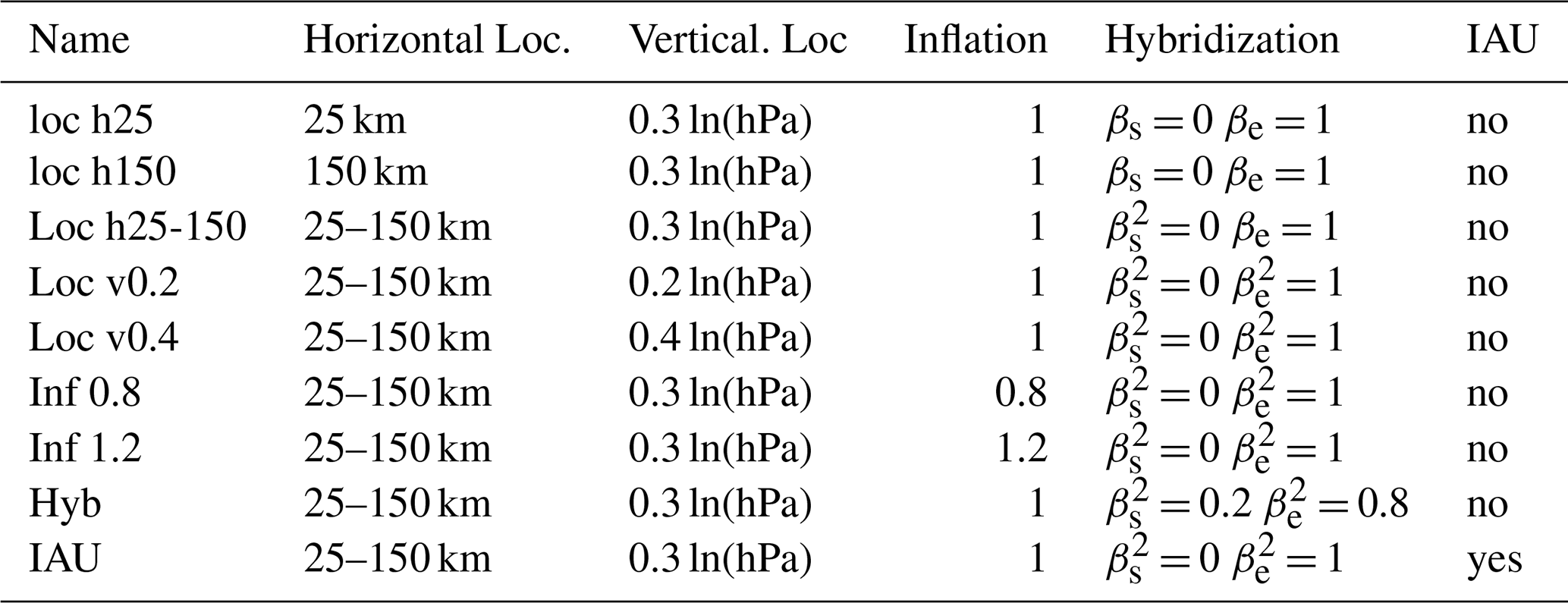
Different parameters have to be tuned in such a 3DEnVar scheme. The authors are aware that all these parameters are linked to each other and that changing one parameter can have an impact on the optimal value of another one. However, the number of experiments that can be run and evaluated is limited. Three different horizontal length scales for the horizontal localization were first evaluated, since in the previous studies MO18 and MI21 this parameter appears to have the most visible impact. Then, different experiments were performed to evaluate the sensitivity to the vertical localization, inflation (i.e. multiplicative factor on background error standard deviations), hybridization (i.e. use of both ensemble and climatological parts in the B matrix representation) and to the use of IAU for initializing the forecast and reducing the spin-up effects. As this section relies on the investigation of forecasts from the DA cycle, the IAU experiment mentioned hereafter incoporates IAU solely to initialize the forecast with the analysis performed at H. No experiment uses IAU to update the forecast initialized at H with the H+1 analysis for long forecasts as explained in Sect. 2.2. These sensitivity experiments, described in Table 1, were run from 13 September to 15 October 2021.

Table 1 Summary of the experiment characteristics used in Sect. 3.

3.2 Horizontal localization length scale

Based on the optimal results of the previous studies, two horizontal length scales constant in the vertical are first evaluated, namely the longer 150 km as in MO18 (experiment Loc h150 hereafter), and the shorter 25 km similar to MI21 (experiment Loc h25 hereafter). O-A and O-B results against 3D-Var (3DVar hereafter) are summarized in the two first lines of each panel of Fig. 3. For both experiments, RMS(O-A) are substantially smaller in the 3D-Var experiment than in the 3DEnVar experiment due to lower σ_b in the flow-dependent 3DEnVar B matrix than in the climatological modelized 3D-Var one: the analysis fits observations to a lesser extent in 3DEnVar. RMS(O-B) are closer between the two compared experiments. In the Loc h150 configuration, the differences reach only 5 % in absolute value. Some are degraded such as for temperature and wind (except at 850 hPa); few are improved. In the Loc h25 experiment, RMS(O-B) values are improved in most of the troposphere but degraded in the high troposphere for both wind and temperature. In order to retain beneficial impacts while avoiding the degradation in upper levels, an experiment using a horizontal localization length scale uniformly varying from 25 km in the lowest vertical level to 150 km in the highest was performed (experiment Loc h25-150 hereafter). This experiment shows lower improvement against 3D-Var than Loc h25 in the low troposphere, but remains better than 3D-Var in the high atmosphere. These results are confirmed by the HSS for 24 h precipitation, simulated by the sum of the 24 1 h range forecasts of the DA cycle for each day (Fig. 4). The three 3DEnVar experiments show better performance than the 3D-Var one (first three columns of Fig. 4). Relative HSS differences are higher than 2 % and can reach around 6 %. They are statistically significant for all experiments and precipitation thresholds. Experiments using the shorter horizontal localization length scales, namely Loc h25 and Loc h25-150, present the best performance. Indeed, both are better than Loc h150 (fourth and fifth columns of Fig. 4) and show very similar performance: the weak differences between these two experiments (sixth column of Fig. 4) are not statistically significant.

3.3 Spin-up investigation

Spin-up here refers to a non realistic propagation of rapid waves in the model, generated by existing imbalances in the model fields. Firstly, it leads, for example, to unrealistic surface pressure tendencies due to gravity wave propagation. In some cases, this phenomenon can also jeopardize the model numerical stability and generate numerical crashes in the case of too large accumulated imbalances. This aspect is investigated by examining the evolution of the RMS of surface pressure tendency averaged over the domain of ten long range forecasts, for the different configurations considered (Fig. 5). For all experiments, each forecast starts with high RMS values, which decrease quickly and regularly during the model integration to reach reasonable values after 2 h of integration. After this forecast lead time, these diagnostic values are very low, as demonstrated by the averaged curves but also the envelope of minimum and maximum values: this suggests that these higher averaged values at the beginning of the forecast are due to imbalances in the model states, and are not an indication of meteorological gravity waves, which could be encountered in a non-hydrostatic model solution. This diagnostic also shows that:

1. the spinup is higher in all 3DEnVar experiments not using IAU than in the 3D-Var one,

2. the shorter the localization length scale is, the faster the spin-up decreases during the first hours of forecast (Loc h25 Versus Loc h150),

3. hybridization helps also to reduce the spin-up,

4. the spin-up level is similar for Loc h25-150 and Loc h150 experiments on this diagnostic,

5. as expected, the use of IAU allows the elimination of this spin-up.

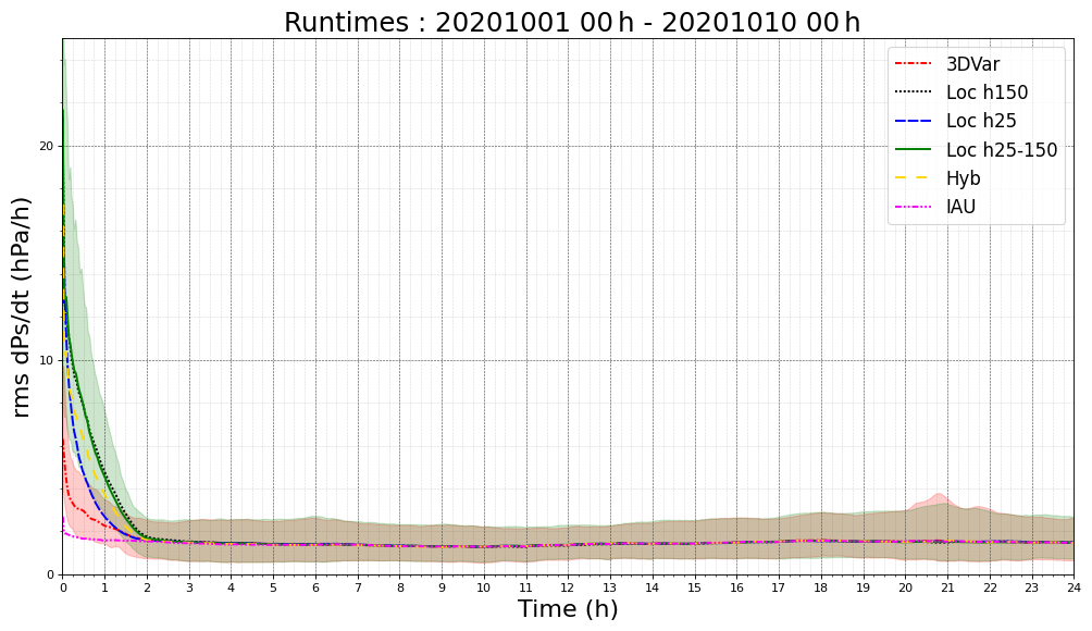
Figure 5 Evolution of the RMS of surface pressure tendency (hPa h⁻¹) over the whole domain at each model timestep during the 24 h forecast ranges averaged over the ten long range forecasts initialized at 00:00 UTC between 1 and 10 October 2020 for 3DVar (dashed-dotted red line), Loc h150 (dotted black line), Loc h25 (short dashed blue line), Loc h25-150 (plain green line) and Hyb (long dashed yellow line) and IAU (dashed-double dotted line) experiments. The envelope of minimum and maximum values is also plotted for 3DVar and Loc h25-150 experiments.

The evolution of the RMS of surface pressure tendency averaged over the domain during several successive forecasts of the DA cycle for the different configurations considered has also been investigated (not shown) and it presents a similar behaviour as in the 24 h forecast. Moreover, while 3DEnVar experiments exhibit higher values at 1 h forecast range than 3D-Var, these higher values are not accumulated through the DA cycle and do not degrade performance as demonstrated in Sect. 3.2.

Finally, the numerical stability aspect is investigated by comparing the number of numerical crashes in the different experiments. Like 3DVar, Loc h25-150 did not crash during the investigated 6-month period, while Loc h150 and Loc h25 experiments crashed both once, during the winter storm Alex on 3 October 2020.

The better results obtained in this study with shorter localization length scales than the optimal ones diagnosed by Ménétrier et al. (2015) could be explained by the fact that, while filtering sampled covariances, the localization helps to improve the analysis quality and the subsequent forecast performance. It also helps to filter the numerical noise due to imbalances in the analysis and thus improves performance of the hourly DA cycle used. MO18 used a 3 h DA cycle and the fast spin-up reduction was not so essential, and MI21 used a hybrid formulation which also helps to reduce spin-up.

Regarding these results, Loc h25-150 shows the best performance for these diagnostics and has been selected as a baseline for the subsequent sensitivity studies.

3.4 Other sensitivity experiments: vertical localization, inflation, hybridization, Incremental Analysis Update

Various experiments were performed to evaluate the sensitivity to the vertical localization, inflation (i.e. multiplicative factor on background error standard deviations), hybridization (i.e. use of both ensemble and climatological parts in the B matrix representation) and to the use of IAU to initialize the forecast and reduce the spin-up effects. In this section, the IAU is used to smooth the imbalances provided by the analysis increment at the beginning of each 1 h forecast from the DA cycle: The new forecast restarts from the background and a constant fraction ($\mathrm{1}/\mathrm{36}$ with a 50 s model timestep during 30 min) of the new analysis increment (analysis minus background) is added to the model solution at the end of each model timestep during the first 30 min of the model integration for the variables of the control vector (u, v, T, q and P_s). The characteristics of the different experiments are summarized in Table 1 and the results compared to the Loc h25-150 experiment are plotted in Figs. 3 and 4. The first result is that the differences obtained on these diagnostics in this section are much smaller than in Sect. 3.2. Relative differences of RMS(O-B), RMS(O-A) and precipitation HSS can be an order of magnitude smaller than the changes provided by the switch from a 3D-Var to a 3DEnVar scheme or by the tuning of the horizontal localization length scale studied in the previous part. Differences are also less often statistically significant. In detail:

• Reducing (respectively increasing) the vertical localization from 0.3 to 0.2 (resp. 0.4) ln(hPa) can provide some weak improvements (resp. degradations). These results are consistent with MI21 (0.25 ln(hPa)) and MO18 (0.3 ln(hPa)) who also diagnosed an optimal value varying from 0.2 ln(hPa) in low levels to 0.4 ln(hPa) in the mid-stratosphere.

• As expected, reducing (resp. increasing) σ_b by a factor of 0.8 (resp. 1.2) leads to increased (resp. reduced) RMS(O-A) as the analyses fit less (resp. more) the observations. The impacts on the subsequent forecasts (the backgrounds) are weak and rarely statistically significant. On these diagnostics, reducing the background error standard deviations, which is a way to compensate for the use of 5, 6 and 7 h forecast range perturbations from the AROME EDA to estimate background error covariances of the 1 h cycle, can provide some slight improvements. Nervertheless, these positive impacts are not propagated to the longer forecast ranges, and lead to a deteriorated performance in the lowest model layers (not shown). A stronger σ_b reduction (inflation factor of 0.5) confirms these worse results (not shown).

• The use of the hybridization (β_e = 0.8 and β_s = 0.2 is illustrated here) can help to slightly improve some O-B values. Nevertheless, It leads to statistically significant weaker performance regarding the HSS of precipitation simulated by the sum of the 1 h range forecasts (Fig. 4). Scores on longer forecast ranges have also been investigated (not shown) and present the same kind of degradation.

• The use of the IAU seems to provide some slight improvements, but once again rarely statistically significant.

Finally, different combinations of values and a mixture of the previous components were also evaluated, but associated impacts are not detailed here. For example, horizontal localization sensitivity experiments using IAU were also performed, leading to the same conclusion concerning the optimal lengths. Localization, by filtering sampled covariances, helps to improve analysis performance and, thus, performance of subsequent forecasts, while it has a weak impact on the spin-up reduction diagnosed on surface pressure tendencies. IAU filters numerical noise introduced by imbalanced analysis increments into the model integration during the forecast step: it has a strong impact on the surface pressure tendency but a weaker one on system performance. Localization and IAU do not filter the same things; they have different impacts on forecast performance and on model stability, while both are useful for the system robustness.

On the other hand, the results of MI21 concerning the better performance provided by a 50 member ensemble versus a 25 member ensemble have also been confirmed (not shown).

3.5 Numerical cost

As in MI21, some adjustments had to be done in order to keep the numerical cost of the new scheme compatible with operational use. The 3D-Var scheme needs a 260 s wall time to perform the analysis with 50 iterations (inner loop) on 8 nodes of the “taranis” Bull Sequana XH2000 platform at Météo-France equipped with AMD Rome technology (AMD EPYC 7742 64 core 2.25 GHz). These 8 nodes offer sufficient memory to allow the reading of the 50 ensemble members in the 3DEnVar scheme. However, the additional time to read these 50 members, estimate the perturbations and mainly apply the localization can increase the wall time up to 600 s. In order to compensate for this increase, the maximum number of iterations in the inner loop is reduced from 50 to 40 without any impact on the analysis quality (not shown). On the other hand, the number of used nodes is increased from 8 to 12 (among the 1152 available) without any impact on the super computer exploitation and side effects on the other components of the NWP system.

3.6 Summary

Using the two diagnostics described above, an “optimal” configuration, hereafter called EnVar experiment has been chosen using:

• a perturbation matrix X from a 50-member AROME-EDA at 3.2 km resolution,

• a varying horizontal localization length scale on the vertical from 25 km at the lowest level to 150 km at the highest,

• a constant vertical localization of 0.3 ln(hPa),

• an inflation factor of 1.0: the dispersion of the 5, 6 an 7 h perturbed forecast ranges from the AROME-EDA is considered to be realistic and still representative of background errors,

• no hybridization.

This configuration has been investigated over a long time period and on the simulation of various severe meteorological events such as winter storms, fog or HPEs. The correct numerical stability of the model dynamic in this configuration has been demonstrated by the fact that no numerical explosion has been reported during more than 1 year of forecast experiment time despite the simulation of numerous storms with strong winds. Surprisingly, this configuration met numerical problems while simulating heat-waves during summer 2022: four 1 h forecasts from the assimilation cycle crashed at the beginning of the model integration in mountainous areas, while the temperature analysis increment provided by surface stations was concentrated near the ground by the flow-dependent background error vertical correlations from the 3DEnVar scheme compared to the climatological 3D-Var ones.

As a precaution, a second configuration was also investigated in parallel. It is called EnVarI in this study, and it uses IAU to smoothly introduce the analysis increment in the first 30 min of the model forecasts in the assimilation cycle, and also in the longer range forecasts.

4 Evaluation of the selected configuration over a long time period

This section presents the results of the comparison between the 3D-Var (3DVar) and 3DEnVar experiments (EnVar and EnVarI) retained after the previous section over a 5.5-month period using different scores. In this section, focusing at 00:00 UTC, the long forecasts initialized at 00:00 UTC are updated with the analysis performed at 01:00 UTC in the three experiments. Only the EnVarI experiment uses IAU to initialize the forecast with the 00:00 UTC analysis.

4.1 Standard scores

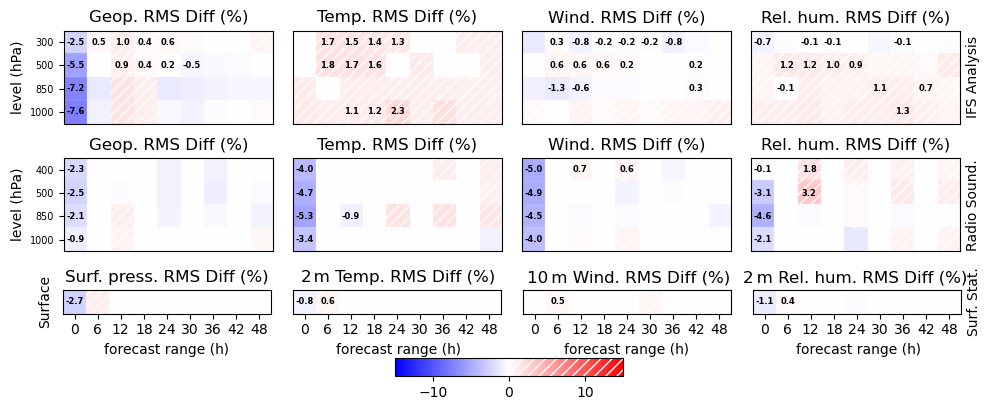
First, classical scores estimated against the ECMWF/IFS analysis, radio-sounding and surface station measurements are evaluated. The relative differences of the Root Mean Square Error between EnVar and 3DVar experiments for different model variables, levels and forecast ranges are summarized in Fig. 6. Concerning the tropospheric fields, EnVar is generally closer to the reference than the 3DVar experiment. Rare exceptions concern geopotential (IFS analysis and radio-sounding) and temperature (only for radio-sounding) at the analysis time, as already seen for O-A values in Fig. 3. This RMSE reduction in the EnVar experiment is higher for lower levels and earlier forecast ranges and decreases when forecast range increases, as the impact of the initial conditions is reduced in long forecast ranges. Using IFS analyses as reference, these differences still reach 5 % for all the fields at 12 h forecast range and 4 % at 24 h forecast range for temperature and specific humidity. Most of these differences are statistically significant (as indicated by the presence of a number in the corresponding boxes), particularly for temperature, wind and specific humidity. Regarding radiosondes, the improvements are weaker but still significant for almost the same forecast range albeit over fewer vertical levels. Concerning surface observations, the behaviour of EnVar is close to 3DVar except at analysis time.

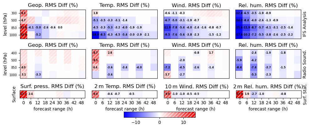
Figure 6 ScoreCard of the relative difference (%) of Root Mean Square Error between 3DVar and EnVar experiments averaged from 15 September 2020 to 1 March 2021, for geopotential and surface pressure (first column), temperature (second column), wind (third column) and relative humidity (last column) against IFS analysis (first row) and radio-sounding (second row) at different vertical levels (y axes), and surface stations (last row) from 0 to 48 h forecast ranges (x axes) every 6 h (12 h for radio-sounding). Negative values (in blue) indicate better performance for the EnVar experiment. Numbers indicate that the difference is statistically significant using a Bootstrap test with 95 % confidence interval.

The use of IAU in the EnVarI experiment, compared to EnVar in Fig. 7, improves the analysis fit to observations. For the other forecast ranges, differences between these two experiments are very much smaller than those with the 3DVar experiment and rarely reach 2 %.

Figure 7 Same legend as Fig. 6 but between EnVar and EnVarI experiments: negative values (in blue) indicate better performance for the EnVarI experiment.

4.2 Precipitation and wind gust probabilistic scores

This first general evaluation is completed using probabilistic scores of precipitation and wind gusts better suited for verification at convective scale than deterministic verification at grid resolution as they take into account the double penalty, which affects classical local scores if e.g. small-scale phenomena like convective cells are predicted well but with some dislocation. The Brier Skill Score (BSS, Amodei et al., 2015) of an event (in general a threshold exceedance) is estimated comparing the frequency of the observation and the simulation of this event in a spatial neighborhood. Relative differences of BSS between 3DVar and EnVar experiments are shown in Fig. 8a for the convective period from 15 September to 1 December 2020 and Fig. 8b for the winter period from 1 December 2020 to 1 March 2021 without neighborhood (in this case BSS is equivalent to HSS) and with a 52.8 km spatial neighborhood. This neighborhood is used to compute the AROME-France Performance Index employed to measure the evolution of the quality of the AROME-France forecasts. This index is computed as the average of the BSS values obtained for precipitation thresholds of 0.5, 2.0, and 5.0 mm 6 h⁻¹, as well as for wind gusts exceeding 40 km h⁻¹, evaluated over forecast ranges of 6, 12, 18, and 24 h. As expected, the BSS comparison between the two periods shows that the 3DEnVar analysis has a more important impact during the convective period, as initial conditions have a larger influence on the simulation than during the winter period. This impact is visible for all precipitation thresholds. It is weaker when using the 52.8 km neighborhood, but it remains statistically significant and higher than 4 % for the 18 h forecast range. For wind gusts, the improvement concerns the lower threshold and is weaker and less significant than for precipitation. However, the improvement provided by the use of a 3DEnVar analysis in the selected configuration is obvious and visible in the AROME-France Performance Index which changes from 0.814 to 0.823 (+1.1 %) during the winter period and from 0.800 to 0.822 (+2.75 %) during the convective one which is consistent with the findings of MI21. Using these scores, performance of EnVarI is very close to that of EnVar and is not shown or discussed here.

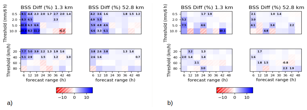
Figure 8 ScoreCard of the relative difference (%) of Brier Skill Score between 3DVar and EnVar experiments averaged from 15 September to 1 December 2020 (a) and from 1 December 2020 to 1 March 2021 (b) for 6 h precipitation against ANTILOPE radar/raingauge blended product (first row) and 6 h maximal wind-gust against surface stations (second row) for different threshold (y axes: 0.5, 2, 5 and 10 mm 6 h⁻¹ for precipitation, 5.6, 11.1, 16.7, 22.2 m s⁻¹) from 0 to 48 h forecast ranges (x axes) every 6 h estimated without (first column) and with a 52.8 km spatial neighborhood (second column). Positive values (blue) indicates better performance for the EnVar experiment. Numbers indicate that the concerned difference is statistically significant using a Bootstrap test with a 95 % confidence interval.

As shown in this section, the retained configuration exhibits better general performance than the operational 3D-Var. It is now evaluated on its ability to simulate particular meteorological events: fog and storm cases during winter, and Mediterranean High Precipitating Events during autumn.

5 Evaluation for severe meteorological situations

5.1 Winter storms

The performance of the 3DEnVar configuration on the prediction of storms and particularly on the intensity of wind gusts was evaluated for 6 winter storms over the French territory and compared to that from the 3D-Var. For each storm, 48 h forecasts are computed every hour starting from an analysis from the hourly DA cycle. A large sample of long-term forecasts is thus available over the period of the event. Contingency table scores for 80 and 100 km h⁻¹ wind gust thresholds are calculated using French surface station measurements for the different forecast ranges (1, 2, 3, 6, 9, 12, 15, 18, 24, 30 and 36 h) which have a validity time during the storm period. The following storms are studied: Daniel, from 16 December 00:00 UTC to 17 December 2019 12:00 UTC (36 forecasts), Fabien, from 21 December 12:00 UTC to 22 December 2019 18:00 UTC (30 forecasts), Jorge, from 27 February 00:00 UTC to 28 February 2020 00:00 UTC (24 forecasts), Alex, from 1 October 00:00 UTC to 2 October 2020 00:00 UTC (24 forecasts), Barbara, from 20 October 12:00 UTC to 21 October 2020 18:00 UTC (30 forecasts) and Bella, from 27 December 00:00 UTC to 29 December 2020 00:00 UTC (48 forecasts).

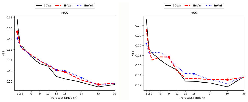
Figure 9 HSS for 80 km h⁻¹ (left) and 100 km h⁻¹ (right) wind gusts simulated during 6 winter storms over the french territory (Daniel, Fabien, Jorge, Alex, Barbara and Bella) by hourly initialized forecasts as a function of the forecast range (h) for 3DVar (plain black line), EnVar (dashed red line) and EnVarI (dotted blue line) compared to surface station measurements. Colored dot above the lines indicates that the HSS difference with the 3DVar experiment is statistically significant for the indicated forecast range using a bootstrap test with a 95 % confidence interval.

For instance, for storm Daniel the 1 h HSS is estimated from the 1 h forecast range from each of the 36 forecasts starting between 15 December 23:00 UTC and 17 December 11:00 UTC, the 2 h HSS is estimated from the 2 h forecast ranges from the 36 forecasts starting between 12 December 22:00 UTC and 17 December 10:00 UTC … and the 36 h HSS, is estimated from the 36 h forecast ranges from the 36 forecasts starting between 14 December 12:00 UTC and 16 December 00:00 UTC. 192 different forecasts are thus used to estimate the Frequency Bias (not shown) and the HSS presented on Fig. 9. For both thresholds and all forecast lead times, the two experiments are very close in average. There are few differences over the first forecast ranges, for which 3DVar performs better, possibly due to dynamical fields being affected by a higher and longer spin-up in EnVar and EnVarI. Fortunately, this longer spin-up does not have a negative impact on longer forecast ranges and EnVar can be slightly better (at 15 or 18 h for 80 km h⁻¹ or 9 h for 100 km h⁻¹). On average, the three experiments seem to present similar performance. This result is not surprising as this kind of meteorological event is driven by large scales and limited area analyses at smaller scales are not expected to be decisive. However, the fact that the smaller scales analyzed with 3DEnVar, and the associated spin-up increase, do not degrade the wind gust simulations, is a very interesting result. The use of IAU in EnVarI provides similar results except at 1 h forecast range which shows a higher degradation than EnVar. At the other forecast ranges, the differences with 3DVar remain very close, even if the statistical significance of these differences can vary from one experiment to another.

5.2 Fog events

Unlike winter storms, fog events are very sensitive to very local conditions. Therefore, the improvement of their simulations can be expected when using a 3DEnVar analysis, e.g. through vertical error correlations in lower layers, which are more representative of temperature inversions involved in this kind of situation. The ability to simulate fog events has been evaluated in the framework of the SOFOG3D field campaign (Burnet et al., 2020), which took place in the south-west of France during winter 2019–2020. 48 h forecasts were performed starting at 18:00, 20:00, 22:00, 00:00, 02:00, 04:00 and 06:00 UTC during the nights when stable winter conditions, favourable to fog formation, were expected. In addition, Intense Observation Periods (IOPs) were carried out during the SOFOG3D field campaign, whether the fog was observed or not, in order to measure detections, non detections but also false alarms. 3D-Var and 3DEnVar experiments have been evaluated by computing contingency tables of fog occurrence. Observations came from the French surface stations (a visibility lower than 1000 m being considered as a fog event) and the simulations were deduced from a new visibility diagnostic calculated using a second degree polynomial relation that links 6 months of observed visibility to AROME-France forecasts of liquid water and rain contents (Ingrid Etchevers, personal communication, 2021). Frequency Bias (the closer the frequency bias value is to one, the better the forecast performance) and HSS (the higher the HSS value, the better the forecast performance) for the event “visibility lower than 1000 m” are presented in Fig. 10. Both 3DEnVar experiments (EnVar and EnVarI) perform better than 3DVar for both scores and the HSS differences are statistically significant for the first 14–16 h forecast ranges.

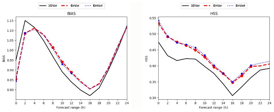
Figure 10 Frequency Bias (left) and HSS (right) for fog events (visibility lower than 1000 m) simulated by forecasts initialized at 18:00, 20:00, 22:00, 00:00, 02:00, 04:00 and 06:00 UTC during 16 nights of the SOFOG3D field campaign IOPs as a function of the forecast range (h) for 3DVar (plain black line), EnVar (dashed red line) and EnVarI (dotted blue line) experiments compared to surface station measurements. Colored dots above the lines indicate that the score difference with 3DVar is statistically significant for the indicated forecast range using a bootstrap test with a 95 % confidence interval.

5.3 High Precipitating Events over the Mediterranean area

The improvement of the simulation of High Precipitating Events (HPEs) is one of the main goals of a convective scale DA system such as AROME-France. This kind of meteorological event is an important issue for weather forecasting in the south of France as they lead to severe damage and numerous casualties. They occur regularly over these French regions in autumn when low geopotential areas over the near Atlantic or the Iberic peninsula generate low-level southerly flows, which bring hot and moist air masses from the Mediterranean sea. The latter generate strong convective events when they meet the first hilly areas. The main difficulty is to evaluate if this strong convection will remain in the mountainous areas or will give stationary precipitation over more populated areas near the Mediterranean seaboard. A 3DEnVar configuration is first evaluated on 7 HPEs during autumns 2020 and 2021. The behavior of the data assimilation cycle itself is investigated by comparing the observed rainfall and the sum of the 1 h forecasts from the DA cycle, as mentioned in Sect. 3.1. As a second step, long-term forecasts are investigated. As the predictability of such events is very low, it is not sufficient to compare one or two forecasts from different experiments to be able to conclude about their respective performance. In this study, each event is investigated using a lagged ensemble approach: the simulation of the HPE is repeated 16 times for each experiment, using long-term forecasts initialized with successive hourly analyses from the DA cycle. The experiments are evaluated using the full sample in order to obtain a robust comparison. EnVar and EnVarI experiments present very similar performance and only EnVarI is compared to the 3DVar one in this section.

5.3.1 The 19 September 2020 case in detail

The first event investigated occurred on 19 September 2020 in the Gard region and gave more than 500 mm in 20 h over the same limited mountainous area. Damage was not so severe as this is not an urban area, but important cities are not very far away and a slight difference in the location of the maximum of precipitation, as simulated by some of the operational AROME-France runs, would have had a higher impact. The uncertainty of the location of this huge amount of precipitation is an important issue for forecasters in terms of forecasting and warning.

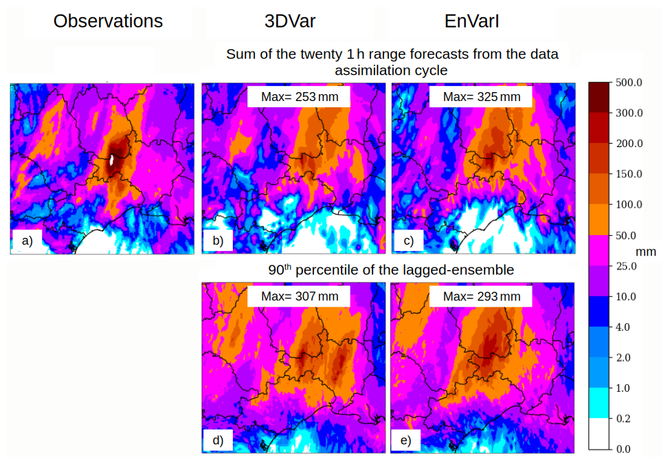
Figure 11 Total rainfall between 19 September 2020 at 04:00 UTC and 20 September 2020 at 00:00 UTC measured by the blending product (radar and rain-gauges) ANTILOPE (a) and simulated by the sum of the twenty 1 h forecast ranges from the DA cycle for 3DVar (b) and EnVarI (c) and the 90th percentile of the lagged-ensemble built with the sixteen long-term forecasts hourly initialized from 18 September 2020 at 13:00 UTC to 19 September 2020 at 04:00 UTC for 3DVar (d) and EnVarI (e).

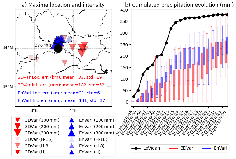
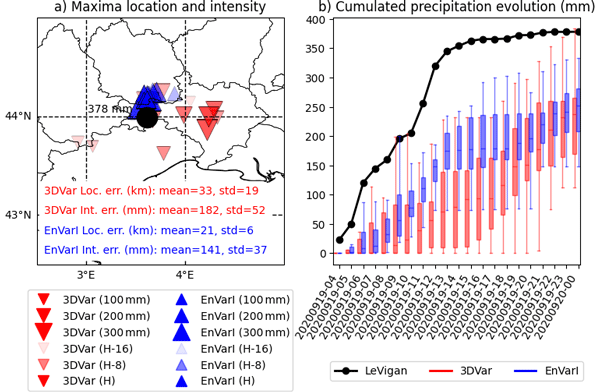
Figure 12 19 September 2020 event: maxima location and intensity for each member of the lagged-ensemble (a) and temporal evolution of the maxima intensity during the forecast (b) measured by Le Vigan rain gauge (black dot) and simulated from 19 September, at 04:00 UTC to 20 September, at 00:00 UTC by each member of the lagged-ensemble by 3DVar (red bottom triangle/boxplot) and EnVarI (blue up triangle/boxplot) experiments using forecasts initialized from 18 September 13:00 UTC (H-16) to 19 September 04:00 UTC (H).

First, the total rainfall observed by the blended product ANTILOPE (based on radar and rain gauges) between 19 September at 04:00 UTC and 20 September 2020 at 00:00 UTC (Fig. 11a) is compared to the sum of the 1 h range forecasts from the DA cycle (Fig. 11b, c). Both 3DVar and EnVarI experiments are able to forecast the correct location of the maxima, but its intensity is underestimated in 3DVar as it reaches only 253 mm, far from the 500 mm observed in the blended product or the 378 mm actually measured by the rain gauge of Le Vigan station (Fig. 12). On the other hand, the EnVarI experiment reaches 325 mm. This result shows that 3DEnVar is able to simulate the phenomenon, even in the shorter lead times, with a better intensity than 3D-Var. Longer forecasts from the lagged-ensemble are investigated using ensemble diagnostics. The 90th percentile of precipitation is plotted and compared to ANTILOPE product on Fig. 11d, e. While the 3DVar experiment exhibits 2 maxima of precipitation, the successive EnVarI simulations are more consistent with each other and mainly target the observed location. However, the intensity of the maxima remains close in the two experiments and differences are not statistically significant. Going further, the location of the maximum of precipitation for each forecast of the lagged ensemble built from the 3DVar and EnVarI experiments is plotted on Fig. 12a; moreover, the temporal evolution of these maxima during each forecast is plotted also for both experiments using box plot on Fig. 12b, in order to compare the simulated intensities and their dispersion. For each lagged-member the location error (the distance between the observed and simulated maximum position) and the intensity error (difference between the observed and simulated maximum intensity) is estimated and their mean and standard deviation for each experiment are indicated on Fig. 12a. The results confirm the general better accuracy of the location of the event in the EnVarI experiment. Mean and standard deviation of the location error reach respectively 33 and 19 km in the 3DVar experiment and are reduced to 21 and 6 km in the EnVarI one. EnVarI also exhibits higher intensities (the size of the triangle indicating the position of the maximum is proportional to its intensity). The intensity error mean and standard deviation are also reduced from 182 and 52 mm in 3DVar to 141 and 37 mm in EnVarI. The lagged-ensemble approach also makes it possible to evaluate the ability of the system to converge toward a realistic solution while the data assimilation cycle progresses. In Fig. 12a, the color shade of the triangle depends on the analysis time used to start the forecast: the darker the shade, the more recent the analysis. Thus, the general tendencies along the different analysis times of the location and intensity errors can be estimated. Both experiments exhibit negative tendencies of intensity error: the more recent lagged-members simulate higher intensity, as also illustrated by the larger size of the darker (more recent) triangles. The location error tendency is also slightly negative for the 3DEnVar experiment and actually, the more recent maxima are closer to the observed location than the older ones. This is not the case for the 3D-Var experiment: the general location error tendency is positive large and recent maxima can be located far from the observed position. Figure 12b confirms that EnVarI is able to simulate higher intensities and maximum rainfall. Moreover, the temporal evolution shows that the higher values for 3DVar are obtained thanks to the simulation of a second precipitating period during the second part of the event which is not observed, according to the rain-gauge measurements at Le Vigan (black dotted line) and less visible in the EnVarI experiment.

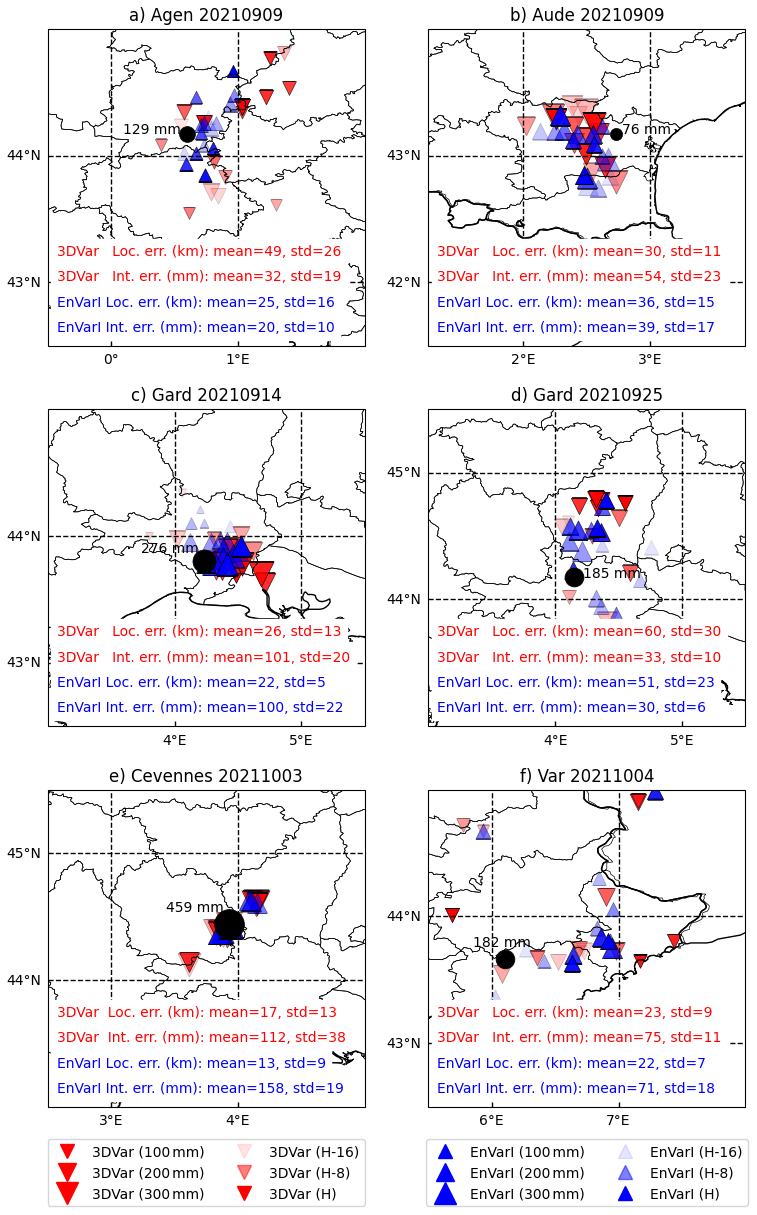
Figure 13 Same legend as Fig. 12a but for HPE observed and simulated on different areas for panels (a) and (b) from 8 September 2021 at 18:00 UTC to 9 September 2021 at 06:00 UTC by 16 forecasts hourly initialized from 8 September 03:00 UTC (h-16) to 8 September 18:00 UTC (h), for panel (c) 14 September 2021 from 06:00 to 12:00 UTC by the 16 forecasts hourly initialized from 13 September 2021 at 15:00 UTC (h-16) to 14 September 2021 at 06:00 UTC (h), for (d) from 25 September 2021 at 12:00 UTC to 26 September 2021 at 12:00 UTC by the 16 forecasts hourly initialized from 24 September 2021 at 21:00 UTC (h-16) to 25 September 2021 at 12:00 UTC (h), for (e) from 3 October 2021 at 00:00 UTC to 4 October 2021 at 00:00 UTC by the 16 forecasts hourly initialized from 2 October 2021 at 10:00 UTC (h-16) to 3 October 2021 at 00:00 UTC (h), and for (f) from 4 October 2021 at 06:00 UTC to 5 October 2021 at 06:00 UTC by the 16 forecasts hourly initialized 3 October 2021 at 15:00 UTC (h-16) to 4 October 2021 at 06:00 UTC (h).

5.3.2 Summary of the other cases

Similar studies, using the same tools, were performed on seven other HPEs. The results of the comparison between 3DVar and EnVarI are illustrated in Fig. 13, except for the event that occurred on 2 October 2020.

• 2 October 2020 (not shown): Storm Alex generated a HPE over the Alpes-Maritimes area which caused severe damage and casualties (Vésubie valley disaster). Unlike the 19 September case, this event is driven by large scale conditions and its predictability is high. The operational 3D-Var AROME-France system was efficient and forecasters could trigger an appropriate warning. 3DEnVar experiments perform as well as the 3D-Var one, both in location and intensity of the event.

• 9 September 2021 (Fig. 13a and b): this event affected two different areas. The 3D-Var operational system encountered two difficulties: the non-detection of a stationary thunderstorm over the town of Agen and a false alarm due to the simulation of a HPE over the Aude region which was not observed (only 76 mm were measured), bearing in mind that this area was strongly affected by severe flash-flooding during October 2018. For both issues, EnVarI performs better than 3DVar: the stationary cell over Agen is, on average, simulated with a better location and intensity. Over the Aude area, the intensity is less overestimated.

• 14 September, 25 September, 3 October 2021: these 3 events affected the Gard region. The stakes were the same as for the 19 September 2020 event: the issue is to correctly estimate the location and the intensity of the maximum rainfall over the plains (14 September, Fig. 13c) or the mountainous and less urbanized areas (25 September, Fig. 13d and 3 October, Fig. 13e). The higher dispersion of the ensemble for the 25 September event indicates a higher uncertainty than for the two others events. For this aspect, the 3DVar and EnVarI experiments have equivalent performance, but EnVarI presents a better location and the reduction of the location error along the analysis time is better for these three events (darker triangles are closer to the observed maxima in EnVarI than in 3DVar).

• 4 October 2021 (Fig. 13f): the weather situation encountered the day before continued, with important rainfall over the Var region, which was not correctly simulated by the 3D-Var operational system. 3DEnVar (EnVarI) helps to simulate more realistic intensities and to target the hinterland areas, even if it is sometimes too eastward.

All the cases studied suggest that the retained EnVarI configuration generally makes it possible to improve the simulation of HPEs compared with the 3DVar configuration, even if this is not systematic. More accurate analyses that are more representative of the small scales involved in such phenomena explain these results. The results of the EnVar experiment are not shown here but are very close to those of EnVarI.

5.3.3 Impact on the system jumpiness

Jumpiness here refers to the run-to-run consistency (or lack of) and the fact that, for the same event, different successive forecasts produced by the same NWP system can differ more or less, depending on the predictability of the event. Investigations into these seven HPE cases indicate that 3DEnVar can help to reduce the jumpiness (i.e. improve the run-to-run consistency) of the AROME-France system. The forecasters subjectively reached the same conclusion when comparing the operational AROME-France (3D-Var) and its E-suite using 3DEnVar, during the period when both sets of runs were available for other HPE cases. In order to objectively measure this improvement, correlations between the accumulated precipitation fields, respectively observed by the ANTILOPE product and simulated by the different hourly initialized forecasts (from H, the most recent, to H-15, the oldest), both valid at the same time, were computed for the 3DVar (a) and EnVarI (b) experiments. The results have been averaged over the 8 HPEs described in this section, and they are plotted in Fig. 14. The first column corresponds to correlations between the observation fields and the different lagged forecast fields: it can be noticed that the correlation increases when the forecast is more and more recent (from h-15 to h) appearing somewhat more clearly in EnVarI than in 3DVar. Moreover, correlations between the different forecast fields (columns h to h-15) appear to be larger in the EnVarI experiment for all the analysis times considered, regardless of the delay between successive analysis times. For example, correlations between forecasts initialized by 3 h lagged analyses (3rd off-diagonal lines) are always larger than 0.65 in EnVarI, while the correlation between forecasts initialized by 1 or 2 h lagged analyses (1st and 2nd off-diagonal lines, respectively) rarely reach this value in 3DVar.

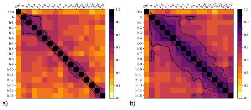
Figure 14 Correlations between accumulated precipitation field observed (first column: ANTILOPE blended product) or simulated by the different hourly initialized forecasts (h to h-15 columns) valid at the same time for 3DVar (a) and EnVarI (b) experiments averaged on the 8 HPE observed and simulated on different areas for 19 September–3 October 2020 and 9 September, 14 September, 25 September, 3 October and 4 October 2021.

6 Conclusion

After 15 years of operational runs, a major update of the AROME-france DA scheme occurred in October 2024: the historical 3D-Var scheme was replaced by 3DEnVar, including fully flow-dependent background error covariances, which was achieved after several years of thorough studies and experiments. While preliminary investigations have already been described in MO18 and MI21, the purpose of the present paper is to describe the set of studies which were conducted in order to achieve this operational implementation.

The first part describes the complex current operational NWP system used at Météo-France in which the new scheme has been included, paying particular attention to its interactions with existing LAM EDA and EPS applications. Operational constraints require that the AROME-France 3DEnVar uses forecast perturbations from the AROME EDA in an asynchronous way: H-1, H and H+1 3DEnVar analysis times use 5, 6 and 7 h range perturbed forecasts from the H-6 EDA analysis time.

The second part of the article is devoted to fine-tuning the different elements of the 3DEnVar scheme itself. Several sensitivity studies were performed and evaluated using diagnostics relevant for the DA cycle. Among these various elements, the horizontal localization length scale was found to have the largest impact. Best performance was obtained with a length scale varying regularly along the vertical, from 25 km at the lowest model level, to 150 km at the highest. This optimal setting is different from those diagnosed in MO18 (170 km constant over the vertical) or resulting from sensitivity experiments in MI21 (40 km constant over the vertical) in different experimental frameworks. The vertical localization length scale setting is more consistent with these two previous studies, since the value of 0.3 ln(hPa) has also been retained here. Sensitivity experiments to the EDA spread were also performed, by modifying the multiplicative inflation factor. The purpose of such a modification would be to compensate possibly for the use of 5, 6 and 7 h forecast ranges from the EDA to estimate the 1 h background error covariances of the hourly DA cycle of the deterministic system; in the end, the obtained optimal value of 1 confirms that the spread of the ensemble of perturbations used is quite correct. As in MO18, the use of a full ensemble-based B matrix (no hybridization) was also found to provide the best results. This is very important as it makes further developments easier, such as the extension of the control variable to new variables (hydrometeors, non hydrostatic variables) or to the temporal dimension (4DEnVar), since relevant flow-dependent background error covariances are directly available from the EDA. Finally, the use of IAU was evaluated in order to reduce the spin-up, which is higher in 3DEnVar experiments than in the operational 3D-Var.

As a result of these investigations, a configuration, declined in two versions – without and with IAU, was retained and evaluated over a long period and for different meteorological events. Several averaged scores (against IFS analysis, radiosondes, surface stations) indicate that 3DEnVar outperforms the operational 3D-Var for all parameters in the troposhere at numerous forecast ranges. An outstanding example is the RMSE improvement of relative humidity at 850 hPa against IFS analysis (resp. radiosondes) reaching 8.7 % (resp. 7.4 %) at 12 h forecast range, 4.1 % (resp. 3.7 %) at 24 h forecast range and 2.5 % (resp. 1.5 %) at 36 h forecast range. The simulation of different weather events is significantly improved with 3DEnVar. Results for rainfall and wind gusts are also better. The improvement of the official performance indicator of the AROME-France NWP system, which accounts for the forecast quality of precipitation and wind gusts, reaches 1.1 % during the winter period and 2.75 % during the convective one.

In addition, the simulation of the strongest wind gusts during 6 winter storms is not affected by the higher spin-up in 3DEnVar. Finally, meteorological events sensitive to small scales, such as winter fog (16 IOPs in the SOFOG3D campaign) or Mediterranean HPEs (7 cases during the autumns of 2020 and 2021) are better simulated thanks to the 3DEnVar analyses. Regarding the simulation of these HPEs, the run-to-run consistency is also improved using 3DEnVar.

Due to the improved quality of the control 3DEnVar analysis, to which initial perturbations are added, significant improvements in the performance of the AROME-EPS system has also been observed. In addition, improvements of the AROME-France short-range forecasts (2 to 7 h) that are used as backgrounds in the nowcasting version of AROME-France (AROME-NWC) also have a positive impact on the performance of AROME-NWC (personal communications).

These results have allowed the 3DEnVar to become the new version of the DA scheme for the operational AROME-France NWP system. The retained configuration exhibits a good numerical stability after having run for more than a year. Yet the heat waves over France in the summer 2022 revealed some very rare weaknesses: four 1 h forecasts of the DA cycle crashed as very strong temperature increments appeared in some points of an Alpine Valley in the two lowest model levels, due to very narrow vertical background error correlations. For this reason, the IAU flavour of the defined configuration was finally preferred, as it simulates this period without any problem, leading to its operational implementation on 15 October 2024.

This major change, combined with the use of OOPS, offers interesting prospects in terms of development. On one hand, the scheme itself can benefit from the use of a Scale Dependent Localization (Caron et al., 2019), which is a way to introduce some flow dependency in the specification of the localization length scale: different localization length scales are allowed and are more or less active, according to the scales involved in the meteorological situation. Increasing the ensemble size can also be investigated using lagged- (Caron et al., 2019) or shifted-approaches in order to reduce the impact of sampling noise. Adding hydrometeors in the control vector (Destouches et al., 2023) opens the way for investigations related to direct assimilation of radar reflectivity, in order to replace the current retrieval approach, as well as lightning observations (Combarnous et al., 2024). A major improvement is also expected from the shift towards a 4DEnVar system in order to assimilate radar, SEVIRI radiances, and surface station observations every 15 min in the 1 h DA cycle (at H-30 min, H-15 min, H and H+15 min). In this case, the temporal dimension along the assimilation window is managed by using a 4D state built with the 3D states from the non linear-model at the different timeslots, and using background error temporal correlations between these different 3D states directly estimated from the EDA. First investigations demonstrate that the 4D increment involving the five 3D increments along the 1 h assimilation windows every 15 min is temporally consistent even at convective scale. Such a 4DEnVar system is currently evaluated in an AROME-France test suite and shows very encouraging results compared to the operational 3DEnVar. Finally, coupled DA can also be envisaged: preliminary works concerning the ability of an AROME EDA coupled with a 1D Ocean Mixing Layer to estimate background error cross-correlations between variables for the ocean and the atmosphere have been initiated, and first strongly coupled ocean-atmosphere analysis increments have been obtained.