Predicting slope instabilities in Salvador, Brazil, using machine learning and georeferenced data

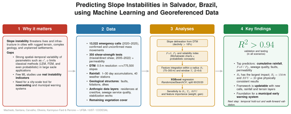
Municipalities worldwide struggle with slope instability, a particularly pressing issue in cities such as Salvador, Brazil, where rugged terrain, escarpments, and complex geology create a high risk of instability. The complexity of the problem is evident in the variability of terrain properties, the bedrock’s inherited structural features, and anthropogenic action. This range of variables makes it well-suited to machine learning (ML) approaches for instability prediction. Although ML has experienced an impressive recent boost, only a few cases have applied ML to real-world instability events. In this paper, a data bank of hydromechanical properties of soils is used in conjunction with a digital terrain model (DTM) and different geo-referenced information, including rainfall, vegetation coverage, geological structures, sewage collection/treatment status, and residential density, to predict the occurrence of soil mass movements and related emergency calls to the municipality from the population living in risk areas. 13 522 emergency calls were considered during the period from 2020 to 2025. Excellent predictive performance, with an R²≈ 0.98 consistently across both the validation and testing phases, was obtained in this original study. This strong result underscores the viability of machine learning as a powerful tool for this kind of problem, particularly within municipal warning systems.

1 Introduction

Slope stability analysis is a key branch of geotechnical engineering, a necessary tool for hazard prediction (Silva et al., 2008; Kinde et al., 2024). It is essential, along with other related knowledge areas such as debris flow (Fannin et al., 2015), to mitigate landslide risks that cause billions of dollars in economic damage annually and threaten lives and infrastructure. Traditional limit equilibrium methods (LEMs), such as Bishop's Simplified Method (Bishop, 1955) and Morgenstern-Price (Morgenstern and Price, 1965), and numerical techniques such as the Finite Element Method (FEM) and Strength Reduction Method (SRM), rely on assumptions about slip surfaces, soil homogeneity, and force equilibrium that struggle with uncertainties in soil properties (cohesion c), friction angle (ϕ), unit weight (γ), geometry (height H), angle (β), pore pressure (r_u), and external factors (seismicity, anthropic actions). c, ϕ, and r_u exhibit significant spatial-time variations (Trinidad and Momayez, 2025; Baecher, 2023), making it challenging to choose typical values for analysis, although they are related to the soil formations of the site and cannot be considered purely random. Several works recognize the importance of spatial correlation of geological properties (Griffiths and Fenton, 2004; Griffiths et al., 2009; Fenton and Griffiths, 2008; Ghasemian et al., 2024). Furthermore, data scattering is linked to the volume of soil mobilized in a test and the smaller the specimen, the greater the variability (Baecher, 2023). Probabilistic methods such as Monte Carlo simulation (Wang and Akeju, 2016; Mehdizadeh et al., 2020; Javankhoshdel and Bathurst, 2014) and the first order second moment (FOSM) (Wong, 1985; Phoon and Kulhawy, 1999) aim to mitigate some of these deficiencies, representing the variability and uncertainty inherent to natural geological structures, despite facing challenges in modeling the complex non-linear interactions that are inherent of the soil/rock masses (Trinidad and Momayez, 2025). Furthermore, the interactions between soil and environment, anthropic factors, and the scale of the simulation have a significant impact on the probability of slope instability events (Neves et al., 2025).

Data-driven based methods, including machine learning (ML), deep learning (DL), and soft computing techniques can leverage simulations, field data, and literature to model slope stability. By predicting the Factor of Safety (FoS) or classifying stability status (e.g., stable, unstable), these approaches offer a powerful, data-centric solution for municipal decision-making in risk-prone areas, particularly when handling large, complex databases. Although many of the published papers deal with ML for FoS prediction (Ahangari Nanehkaran et al., 2022; Yadav et al., 2025), ML techniques have proven applicable in a wide range of geotechnical problems, including landslide susceptibility mapping (Trinidad and Momayez, 2025), illustrating the versatility of ML and identifying opportunities for transference of cross-disciplinary knowledge and enhancement of slope stability analysis in large areas. In this regard, the ML models Random Forest and XGBoost are particularly valuable as they combine multiple learners, reducing overfitting while enhancing generalization in cases with substantial data uncertainty (Trinidad and Momayez, 2025).

However, geohazard research on landslide prediction spans four distinct but often conflated categories that differ fundamentally in their temporal orientation and operational intent, and whose distinctions are essential for accurately positioning the present contribution. Landslide susceptibility mapping estimates the spatial propensity of terrain to experience slope failure based on time-invariant intrinsic factors, without reference to any specific triggering event or time period (Guzzetti et al., 1999; ter Braak and Šmilauer, 2018), and while ML has advanced this field considerably (Merghadi et al., 2020; Reichenbach et al., 2018), susceptibility maps carry no temporal probability statement and cannot support time-sensitive warnings. In the Brazilian context, susceptibility mapping remains geographically concentrated in southeastern states, with northeastern Brazil, including Bahia, comparatively underrepresented in the published literature (Dias et al., 2021)

Retrospective event classification incorporates time implicitly by pairing historical landslide inventory records with the environmental conditions that prevailed at the time and location of each event, training models to discriminate recorded failure events from stable reference cases (Lombardo and Mai, 2018; Pellicani et al., 2017); while methodologically informative, such frameworks yield optimistic performance estimates when spatial autocorrelation between training and test samples is not controlled (Goetz et al., 2015), and do not demonstrate skill on conditions genuinely unknown at the time of prediction. Nowcasting estimates current or imminent landslide activity in near-real-time by combining static terrain and geotechnical susceptibility information with dynamic observed forcing to produce spatially distributed hazard intensity estimates with a temporal horizon of hours to a few days (Baum and Godt, 2010; Piciullo et al., 2018); rainfall intensity-duration thresholds represent the most widely deployed nowcasting approach (Guzzetti et al., 2008; Segoni et al., 2018), and integrating terrain susceptibility into spatially variable threshold derivation has been shown to improve nowcasting performance (Monsieurs et al., 2019). In the Brazilian context, Calvello et al. (2015) evaluated the operational performance of the Rio de Janeiro municipal early warning system over four years, providing the most directly relevant precedent for a city-scale nowcasting framework and establishing performance benchmarks against which the present system should ultimately be measured. Operational forecasting extends nowcasting by coupling landslide models with numerical weather prediction outputs to issue probabilistic hazard forecasts with lead times of one to several days, enabling proactive rather than reactive emergency response (Rossi et al., 2017); in Brazil, CEMADEN (National Center for Monitoring and Early Warning of Natural Disasters) operates a national early warning framework integrating satellite rainfall monitoring with susceptibility zonation across thousands of municipalities, representing the operational infrastructure within which city-scale systems such as the one developed here must ultimately be situated.

Although ML has experienced an impressive recent boost, only a few cases have applied ML to real-world instability events in an operational nowcasting context. In this paper, a data bank of hydromechanical properties of soils is used in conjunction with a digital terrain model (DTM) and different georeferenced information, including rainfall, vegetation coverage, geological structures, sewage collection/treatment status, and residential density, to predict calls from the population living in risk areas to the municipality reporting soil mass movements or the perception of risk indicators. This paper predicts landslide hazards in Salvador, Bahia, Brazil, using machine learning (ML) on georeferenced data, which could be categorized as “Nowcasting” of landslides. The model is trained using a novel data source: emergency calls from residents in areas at risk in Salvador, Bahia, Brazil, one of the few cities in Brazil with a consistent and reliable data set in this regard. Results from shear strength and permeability tests conducted by the geotechnical laboratories of the Federal University of Bahia over the past few decades are also used, along with the city's digital terrain model (DTM), to calculate FoS, the probability of failure, and the reliability index across the entire urban area. The cumulative rainfall over periods ranging from 1 to 30 d prior to each event was estimated using data from 40 weather stations. This was used in conjunction with the mapped geological structures, including faults, foliations, and dikes, as variables influencing slope stability. As anthropic input layers, the presence of residences at both the top and the foot of the slope, as well as the quality of the sewage service around the slope, were evaluated. The developed framework can be helpful for municipalities in risk management activities and can provide a tool for online risk monitoring using rain data from city weather stations. Furthermore, the nature of ML enables frequent updates to the system, changing the DTM, residence, and sewage layers over time, and adding new emergency calls and rainfall data to the machine learning database. This strong result underscores the viability of machine learning as a powerful tool for this kind of problem, particularly within municipal warning systems.

2 Materials and methods

2.1 Soil formations and geological structural aspects

The urban area of the city of Salvador is formed of three geological-geomorphological domains: (i) the Recôncavo Sedimentary Basin; (ii) the Atlantic Coastal Margin; and (iii) the high Salvador. The Recôncavo sedimentary basin, formed from the evolution of the crustal stretching, which caused the fragmentation of the Gondwana supercontinent in the Mesozoic era (de Lima, 1999), is separated from the high Salvador by the main fault (fault 1,1 in Fig. 1) of the region (locally known as the high city and the low city). The high city, where most of the landslides occur, has a complex geological history, with different kinds of metamorphic rocks with high degrees of metamorphism, often cut by diabase and granitic dikes (Barbosa et al., 2005; Souza and Gandolfo, 2012). The metamorphic rocks are essentially (i) orthoderived metamorphic rocks of quartz-feldspathic composition, light to dark gray in color (Souza-Oliveira et al., 2014); (ii) paraderived metamorphic rocks (Souza and Gandolfo, 2012) of dark gray color; and (iii) mafic (metagabbros) and ultramafic (metapyroxenites) enclaves, commonly associated with paraderived granulites in the form of boudins (Souza-Oliveira et al., 2014).

With the separation of the Gondwana supercontinent and the formation of the south Atlantic in the Mesozoic, a brittle phase developed, correlated with the opening of the Brazilian marginal basins, among them the Recôncavo Sedimentary Basin, forming faults and fractures, which can be grouped according to their orientation into:

1. N020°–N030° – faults cidade alta-cidade baixa (high-low city, 1,1 in Fig. 1), Iguatemi (1,2) and Jardim de Alah (1,3) and their reverberations.

2. N120^o–N130^o and N130°–N140° faults parallel to the system Mata-Catú (2) (Barbosa et al., 2005; Nascimento, 2008).

3. N080°–N090° fault of Barra (3).

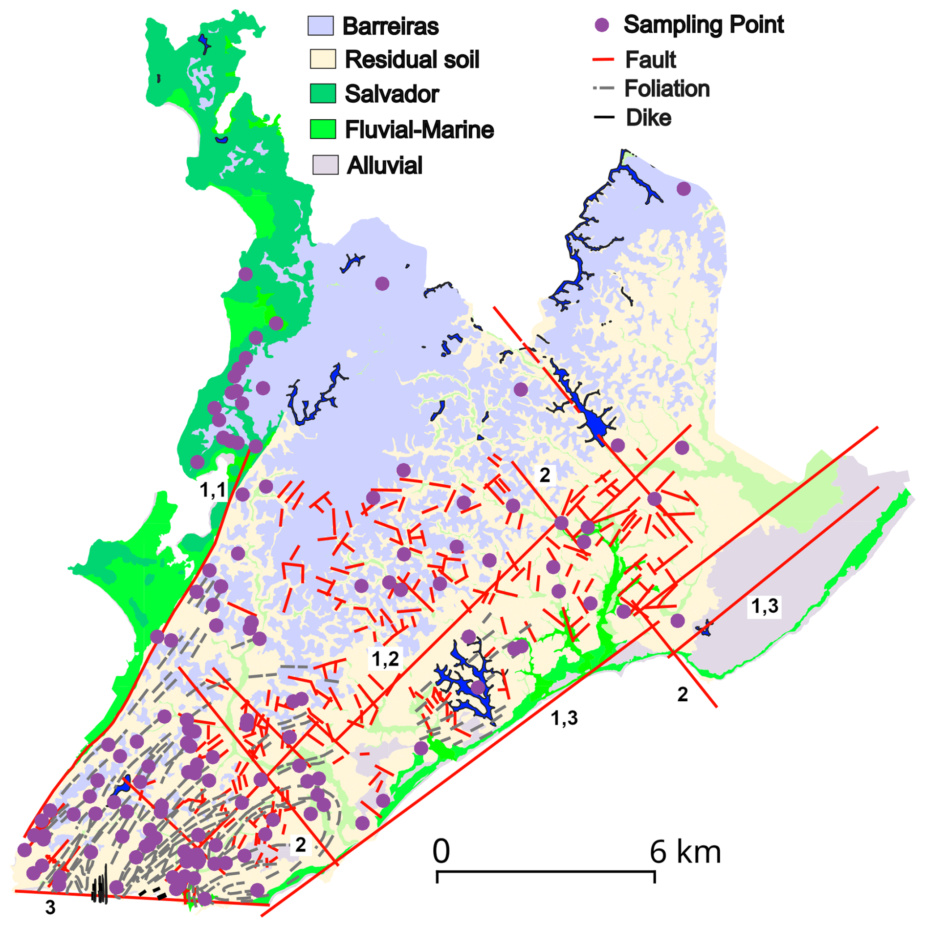
Figure 1 Presence of the main soil formations at surface, sampling points and geological aspects.

Table 1 Databank distribution by formation and geotechnical typical results.

Obs: mean ± SD values.

Table 2 Shear strength parameters and variability of soil formations.

2.2 Databank

The Databank used in the research comprises 350 results of drained triaxial (ASTM-D7181, 2011) and direct shear (ASTM-D3080, 2012) tests performed on saturated and natural water content undisturbed samples collected in the city of Salvador from 2005 to 2022 by Geotechnical (mainly) and Geoenvironmental laboratories of the Federal University of Bahia. Only data providing a satisfactory location (geocoordinates, street address, or a well-known building) were considered. As observed in Table 1 and Fig. 1, most of the data (232 samples) come from the crystalline bedrock's residual soil of Granulite/Gnaisse, which is coherent with the dominant presence of this soil in the urban area. The second most frequently tested formation (68 samples) is the Barreiras sedimentary formation, which typically occupies elevations above 70 m in the city (Fig. 1). These two formations encompass almost the entirety of the slopes analyzed due to their predominance in the superficial soil, particularly in slope areas. The samples of residual of Granulite/Gnaisse presented the highest plasticity and clay & silt content. Apart from the residual soil and Barreiras formations, the Quaternary formations are discontinuous, and the geological map scale can influence the genesis attributed to the samples. Due to the high scattering, the values of k presented in Table 1 express only the order of magnitude of the expected value of permeability for the soil.

Figure 2 Example of slope areas calculation from DTM. (a) resulting streamlines and (b) calculated FoS.

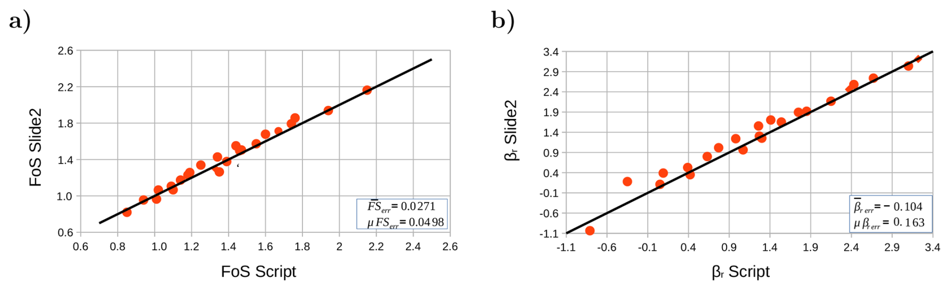
Figure 3 Comparison between developed Python script and Slide2^® (RocScience, 2025) in terms of (a) FoS and (b) β_r.

Reflecting the observed variability in terms of Atterberg limits, soil formations also presented high variability in terms of shear strength parameters (Table 2), mainly for tests performed in natural water content, and for cohesion intercept, since no water content control is applied in the tests (commercial demand of consultants to the laboratories) and the soil's moisture changes over the course of the year. All the formations exhibited high spatial variability, and the different specimen positions in the weathering profile also increased the variability of the residual soils. The idea of the research was to use a Databank that is continuously updated by consultants who require shear strength tests to be conducted at our facilities as part of their activities. Besides the expected values of shear strength parameters, all the observed variability was taken into account in the slope calculation, as discussed below. The correlation coefficient between friction angle (ϕ) and cohesion (c^′), (cor_ϕ−c) was always negative, as reported by many authors in literature (Lumb, 1970; Cherubini, 2000; Wang and Akeju, 2016), however, with different intensities, and was also considered in the performed slope stability calculus. In Table 2, the subscripts nat and sat stand for natural water content and saturated specimens, respectively, and γ is the unit weight of the soil.

2.3 The machine learning model

2.3.1 Input variables

Slope stability results

A Python script was developed to isolate slope areas using the digital terrain model of the city (https://cartografia.salvador.ba.gov.br/dados-geoespaciais/baixar-dados-geoespaciais/, last access: 15 May 2026). The entire city's DTM is of a size of approximately 4.5 GB (54 299×53 010 pixels) and a horizontal resolution of 0.5 m. Areas with a declivity higher than 18 % were isolated, and the top of the slope was identified. Then streamlines were traced at 5 m intervals along the top, and the slope sections were drawn by linking the beginning and end of each streamline (the slope's crest and foot) with a straight line. Using this method, around 775 500 slopes were calculated for the entire city. Figure 2a shows a portion of the urban area where the slope areas were selected and the streamlines traced. For FoS calculation, the slope stability charts by Michalowski (2002) (r_u=0) were digitized and fitted by Eq. (1)

$$\begin{array}{}\text{(1)}& {\displaystyle \frac{\mathrm{FoS}}{\tan \left(\mathit{\varphi }\right)}}=a+{\displaystyle \frac{bx+c{x}^{\mathrm{2}}}{\mathrm{1}+x}}\end{array}$$

where $x=c^{\prime }/\left[\mathit{\gamma }H\tan \right(\mathit{\varphi }\left)\right]$, H is the slope height, FoS is the slope's Factor of Safety and a, b and c are fitting constants for frelieach slope angle (β) of the Michalowski's charts. All the fitted curves had R²>0.999, and the equation's performance was considered adequate. Figure 2b illustrates the slopes and the obtained values of FoS (saturated condition) for the areas illustrated Fig. 2a. Table 3 illustrates the adopted values of a, b and c for each β value and r_u=0. A linear interpolation was adopted between slope angles.

Table 3 Fitting constants for the Michalowski's charts considering r_u=0.

The variability presented in Table 2 for γ, c^′ and ϕ for each condition (natural and saturated) were used with the concepts of the First Order Second Moment method (Wong, 1985) to calculate the FoS's standard deviation (SD, σ) and the probability of failure (PF) of the slope (Eq. 2). The FOSM method is a probabilistic technique for uncertainty and reliability analysis that uses a first-order Taylor series approximation of a function, along with the first and second moments (mean and variance) of the random input variables. This method simplifies reliability analysis by assuming the function can be linearized at the mean values of the inputs and that the output has a normal distribution. It is widely used due to its relative simplicity, however, it can be inaccurate if the function's behavior at the mean is significantly different from the actual value. Despite presenting spatial variability and dependence of the soil's genesis/classification, the unit weight and the shear strength parameters were assumed to be random within the same soil formation.

$$\begin{array}{}\text{(2)}& {\mathit{\sigma }}_{\mathrm{FoS}}=\sqrt{\sum _{i=\mathrm{1}}^n{\left[{\displaystyle \frac{\partial \mathrm{FoS}}{\partial x}}\right]}_i^{\mathrm{2}}{\mathit{\sigma }}_{x_i}^{\mathrm{2}}+\sum _{i=\mathrm{1}}^n\sum _{j(j\ne i)=\mathrm{1}}^n{\displaystyle \frac{\partial \mathrm{FoS}}{\partial x_i}}{\displaystyle \frac{\partial \mathrm{FoS}}{\partial x_j}}{\mathrm{COV}}_{x_i{x}_j}}\end{array}$$

where σ_x is the SD of the variable x (i.e., γ, c^′, and ϕ) and COV${}_{x_i{x}_j}$ is the covariation between the variables x_i and x_j (only the covariance between c^′ and ϕ was considered, using the cor_ϕ−c values presented in Table 2). The $\partial \mathrm{FoS}/\partial x$ values were calculated using the finite difference concept ($\partial y/\partial x\approx \mathrm{\Delta }y/\mathrm{\Delta }x$), varying the values of γ, c^′, and ϕ by 1 % and observing the corresponding variation in FoS.

Once the values of σ_FoS were obtained, the probability of failure was calculated. This was the same as that for obtaining FoS<1 (normal distribution assumed) and the reliability index (β_r) was calculated using Eq. (3):

$$\begin{array}{}\text{(3)}& {\mathit{\beta }}_{\mathrm{r}}={\displaystyle \frac{\mathrm{FoS}-\mathrm{1}}{{\mathit{\sigma }}_{\mathrm{FoS}}}}\end{array}$$

The FoS and β_r values obtained using the script were compared with those by Slide2^® (RocScience, 2025), adopting the Morgenstern and Price (1965) method with a half interslice force function. β values ranged from 30 to 45° and values of H 10–20 m were adopted, with values of c^′ of 5, 15, and 25 kPa and ϕ of 30° and 35°, totaling 48 validation cases. The semi-probabilistic analysis used the Monte Carlo method with a number of samples (N) of 60 000 and the overall slope statistical analysis option, where the entire slip surface search is repeated N times. Some analyses were performed using N>60 000 with no noticeable change in the observed results. As illustrated in Fig. 3, the mean difference in the FoS values between the two methods was ${\stackrel{\mathrm{‾}}{\mathrm{FoS}}}_{\mathrm{err}}=\mathrm{0.0271}$, with a σFoS_err=0.0498, whereas values of ${\stackrel{\mathrm{‾}}{{\mathit{\beta }}_{\mathrm{r}}}}_{\mathrm{err}}=-\mathrm{0.104}$ and $\mathit{\sigma }{{\mathit{\beta }}_{\mathrm{r}}}_{\mathrm{err}}=\mathrm{0.163}$ were rendered, confirming the compatibility between the two methods of analysis.

Figure 4 illustrates some of the input layers and the emergency calls in the period of analysis used in the machine learning process. As observed, most of the emergency calls to the municipality are concentrated in areas with low FoS_sat values. 13 522 emergency calls were analyzed in this paper, including both confirmed and non-confirmed mass movements.

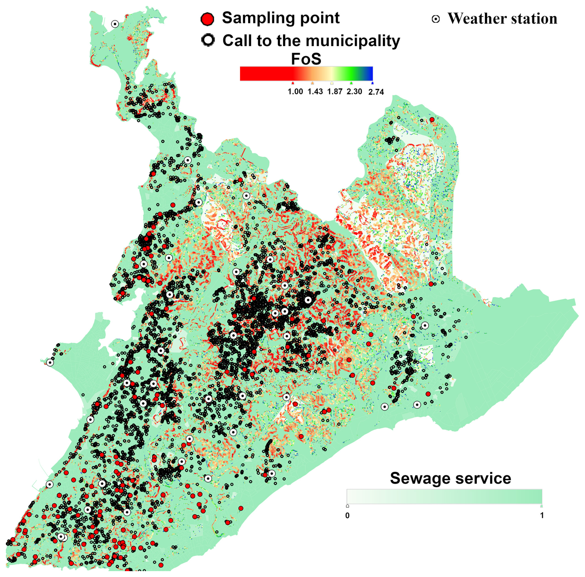
Figure 4 Map with some input layers and the emergency calls to the municipality used to calculate the output variable.

Additional input layers

Besides the values of FoS_sat, FoS_nat, PF_sat, PF_nat, β_rsat and β_rnat calculated for each slope, additional information was used in the machine learning process. For most of the input layers, a radius of influence (R_i) (see Fig. 5) was drawn at the midpoint of each slope to define an area of influence (Ia). Only the georeferenced information inside the Ia was considered in the performed analysis.

Figure 5 Illustration of the calculation process of input and output variables.

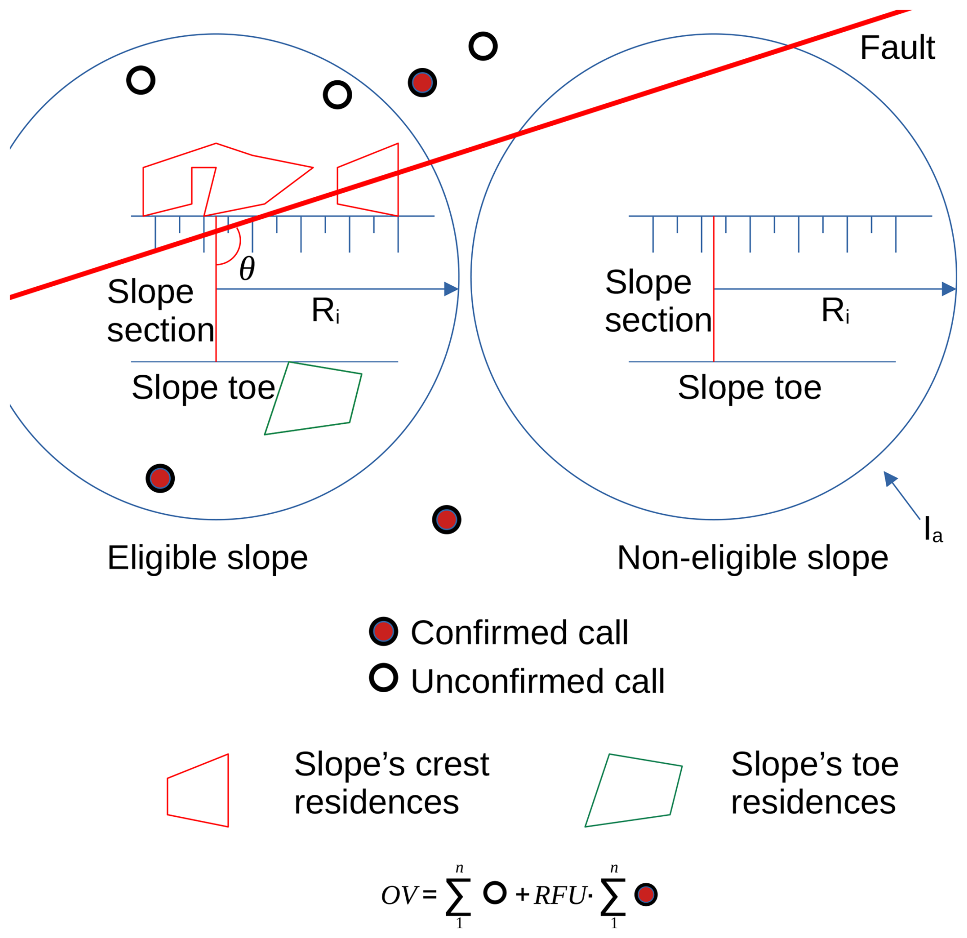
This was the case with the geological aspects of the city. The script searches each eligible slope (slopes having at least one emergency call in the period of analysis inside Ia, as illustrated in Fig. 5) for the geological structures shown in Fig. 1 (faults, foliations, and dikes) and calculates the sine of the angle (θ) between the structure and the line defining the slope itself, generating an input value. The worst scenario occurs when a geological structure intersects the slope direction perpendicularly, having a negligible effect when slope direction and geological structures are parallel. This variable can be considered the complement of the scalar product between the vectors; therefore, the sine of the angles was used in this representation (see Fig. 5). Slopes with no structures inside Ia had a zero structure value. For slopes with more than one structure in the vicinity, the closest structure was considered. Faults, foliations, and dikes were considered separately. As illustrated in Fig. 1, the area of the high city is formed superficially mainly of residual soils from crystalline rock weathering, which contain relic structures that may form preferential failure surfaces, conditioning slope stability (Stead and Wolter, 2015; Santana, 2021).

The presence of residences in the Ia (i.e., Figs. 2a and 5) was also considered using the residence layer provided by the local municipality (https://cartografia.salvador.ba.gov.br/dados-geoespaciais/baixar-dados-geoespaciais/, last access: 15 May 2026). Two input variables were derived as the ratio between the occupied area and the Ia in the slope body and top, and in the neighboring of the slope's foot. This distinction is necessary because the residences located in the vicinity of the slope's foot tend to have a stabilizing effect, in contrast to those observed at the top of the slope and along its length. A further data layer provided by the municipality was the vegetation cover of the slope. In this case, the input variable for each eligible slope was the ratio between the vegetation area and the slope's Ia.

The weather stations presented in Fig. 4 provided hourly information on rainfall in the period of analysis (2020–2025). For each eligible slope, the accumulated rainfall for 1, 2, 3, 5, 7, 10, 15, and 30 d was calculated using as a reference the date of the emergency call and the values recorded in the weather stations, which were interpolated using the inverse of the square distance as weight. All the weather stations provided valid rainfall records on almost all days. In the case of weather stations with no valid data on a given day, the interpolation procedure was performed using the remaining weather stations.

The Brazilian Institute of Geography and Statistics (IBGE) and the Institute for Applied Economic Research (IPEA) published recently data (https://github.com/ipeaGIT, last access: 15 May2026) concerning the quality of the sewage services in Brazil, which is available for analysis using a R^® (R Core Team, 2026) package titled CensoBr (Pereira and Barbosa, 2025). For the city of Salvador, Bahia, information about the sewage system is provided for 4541 census sectors (Fig. 4). For each sector, the quality of the sewage service was evaluated as a weighted mean by the number of residences for the following conditions:

• No sewage collection system and no septic tank or pit – 0

• Sewage disposal in a rudimentary pit – 0.1

• Sewage disposal in a non-engineered septic tank – 0.2

• Sewage disposal in an engineered isolated septic tank – 0.3

• Sewage disposal in an engineered septic tank linked to the sewage collection system – 0.6

• Sewage disposed in the sewage collection system – 1.0

This input variable reflects the development status of the population in the census sector and, to some extent, the presence of the public services. Furthermore, areas with no sewage collection systems (and probably no proper drainage systems) suffer from what may be called anthropic rainfall, as practically all the sewage water infiltrates the terrain along with part of the rainfall.

Finally, in some regions, a preliminary stabilization procedure composed of slope cover with nonwoven geotextile and shotcrete has been applied by the municipality, with potential positive impacts on the slope stability. Therefore, for each eligible slope, the script checks for the existence of stabilization measures prior to the emergence-call date. Only two values are assigned to this variable: 0 or 1.

2.3.2 The output variable and considered scenarios

The output (OV) variable was calculated considering the number of confirmed and unconfirmed calls made to the municipality in the slope's radius of influence and within a time interval (T_i), as illustrated at the bottom of Fig. 5.

Different scenarios performed by varying some analysis parameters were produced for machine learning training. The parameters that were changed in the performed analysis were:

• Slope's radius of influence R_i. Adopted values of 75, 100, 150, 200, and 300 m

• Time interval, in days, before the emergence call date, in which the calls are assumed as part of a unique event. Adopted values of 2–6 d

• Ratio failure/unconfirmed call (RFU) weight. Adopted values of RFU of 5, 10, 20, and 30

During the rainy season, the emergency calls are seldom just received on one single day and may be received over periods longer than one week. Therefore, the machine learning procedures were repeated for different T_i values so as to maximize the R² value in the validation and testing phases of the ML process. Furthermore, only some of the emergency calls were about a mass movement later confirmed in the field by the municipality staff. In order to take this into consideration in the analysis, confirmed calls were given a higher weight (RFU value) in the output variable value, which is calculated as the weighted sum of all the calls in the adopted T_i. Unconfirmed calls were attributed a unity value.

Increasing RFU, T_i, and R_i also increases the value of the output variable. Analysis with a higher R_i will encompass a larger area and involve more slopes per emergency call. The combinations of slopes and emergence calls, for the period of analysis, yielded approximately 872 000 and 11 000 000 observations for values of R_i of 75 and 300 m, respectively, for each RFU, T_i, and R_i, which were modeled as described below. For the same radii cited above, the mean number of slopes embraced by the influence area was 64.5 and 819.

It is important to note that the output variable reflects human reporting behavior, population exposure, accessibility, public awareness, and municipal response practices, not only physical instability. The city of Salvador has implemented warning systems and direct communication channels to reach the population in risk areas. However, the population's perception of risk does not always match with instability events, and when confirmed, landslides exhibit a wide range of scales and impacts, from economic losses to loss of human life. The complexity of the problem is therefore evident, involving geotechnical and geological aspects, the effects of anthropogenic actions, the quality and coverage of public services, and the human response when confronted with risk situations. The use of landslides as an output variable, as adopted in many papers in literature would require deeper investigation of the slip surface geometry, determination of local soil properties, and performing a retroanalysis of the events. The authors believe that the population's perception of risk can be a valuable source of feedback, since they live in such risk areas and, unfortunately, most of them have already experienced such instability events, which helps create a kind of natural perception, being able to analyze local indicators of instability and contact the municipal authorities.

2.3.3 Adopted machine learning procedure

The ML procedure used the XGBRegressor, a Gradient Boosting algorithm based on trees. The XGBRegressor is a class within the XGBoost library that implements gradient boosted decision trees for regression tasks. It is a powerful and popular machine learning algorithm known for its efficiency, flexibility, and performance (Chen and Guestrin, 2016).

Constructing an efficient ANN requires optimizing the various parameters of the model to reach an optimal network configuration. This optimized configuration enables the ML algorithm to establish complex predictive relationships, making ML a powerful and versatile tool in various scientific fields. The optimization process can use empirical (i.e., by trial and error) procedures, which gradually increase the ML model's complexity, or use optimization algorithms, such as Hyperband (Li et al., 2018; Dos Santos Pereira et al., 2025) or the RandomizedSearchCV (Pedregosa et al., 2011).

During the training phase, the RandomizedSearchCV by the scikit-learn library automatically provided the optimized hyperparameters. This method is an alternative to GridSearchCV, and is especially useful when the hyperparameter search space is large. For each R_i, T_i, and RFU combination, the following hyperparameters were optimized seeking the maximum R² of the validation subset: number of boosting trees used (n_estimators) [100, 2500], overly large values can cause overfitting; learning rate (learning_rate) [0.01, 0.5], controls the learning speed. Training is faster with a high value, but might overshoot optimal solutions; maximum depth (max_depth) [3, 15], controls model complexity and training speed; subsample (subsample) [0.1, 0.9], used to build each tree, helping reduce overfitting; colsample by tree (colsample_bytree) [0.1, 0.9], fraction of predictor variables randomly selected for each tree, to reduce overfitting; L1 regularization term (reg_α) [0, 5], to add sparsity and reduce overfitting; L2 regularization term (reg_λ) [0.01, 5]; to improve stability and reduce overfitting; minimum sum of instance weights [1, 10], required in a child node, limiting overly specific tree splits; maximum number of bins [256, 2048], used in the tree splits. The final optimized model adopted the following hyperparameter values: n_estimators =2310, learning_rate =0.1186, max_depth =13, subsample =0.9674, colsample_bytree =0.9552, reg_alpha =3.6742, reg_lambda =1.5491, min_child_weight =3, and max_bin=1353. The XGBoost regressor was configured with the gbtree booster, reg objective function, and hist tree construction method.

For each combination of RFU, T_i, and R_i, the Databank was stratified based on the values of the output variable into 10 classes using 10 percentiles (from 10 % to 90 %), and then randomly split into subsets with 60 % (training), 20 % (validation), and 20 % (testing) of the whole Databank. The test subset remained unseen by ML model during the entire training procedure.

3 Results and analysis

Figure 6 summarizes all the obtained results in the machine learning attempts performed. As observed, in all the scenarios, ML was able to deliver a very good and similar performance for the testing and validation Databanks, with values of R²>0.94.

Figure 6 ML performance for (a) R_i=75 m; (b) R_i=100 m; (c) R_i=150 m; (d) R_i=200 m and (e) R_i=300 m, with varying T_i and RFU.

= Table 4 summarizes the best results obtained for each R_i presented in Fig. 6, and Figs. 7 and 8 illustrate how the slope's radius of influence and RFU impact the ML performance. As observed, R_i had the greatest impact on ML predictive ability, with the highest R² values obtained for R_i=300 m. Furthermore, the influence of RFU and T_i, indicated by the dispersion bars, decreases with R_i. However, using such a large radius of influence may capture emergency calls from adjacent areas and relatively distant structural aspects of the bedrock, as illustrated in Fig. 9, where circles with R_i of 150 and 300 m were traced in a typical area of risk in the city. To further analyze the relative size of the employed radii, they were compared with the distances between the centroids of nearest slope areas.

Figure 10 illustrates the obtained results. As observed, only 24 % of adjacent areas have distances less than 75 m, with 43.1 % of the distance between the nearest areas being less than 100 m.

Using a RFU =20 led to slightly better results for all the R_i. Using a time interval of 4 d, in most cases, resulted in a better performance, although the T_i influence was considered negligible. Figure 6a presents the ML performance for a R_i=75 m with varying T_i and RFU, chosen as the best option in terms of R_i considering the individuality of each slope area.

Table 4 Best machine learning performances for each radius.

Figure 7 ML performance as a function of R_i.

Figure 8 ML performance as a function of RFU.

Figure 9 Illustration of the R_i effect merging data from different adjacent slopes.

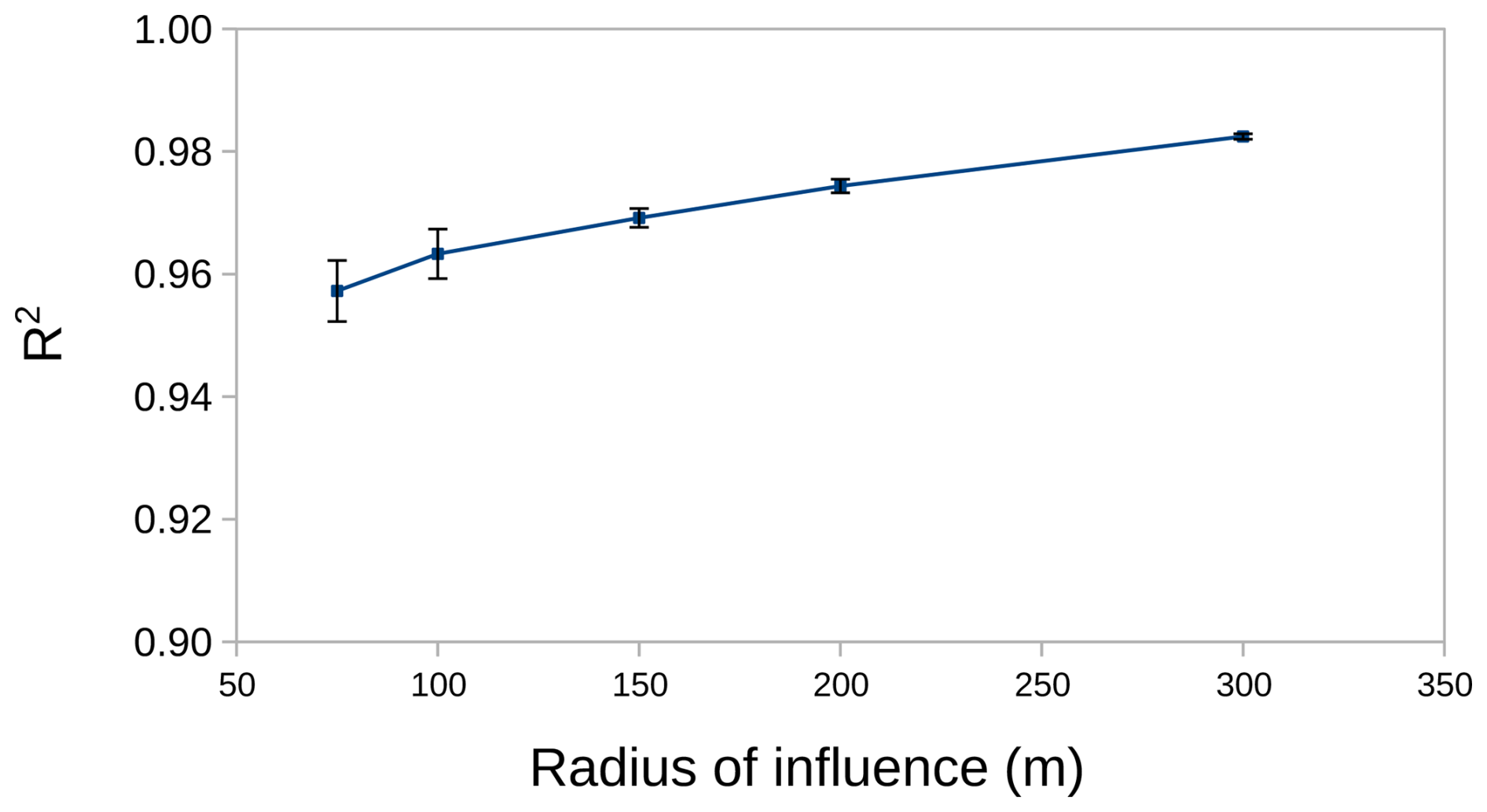
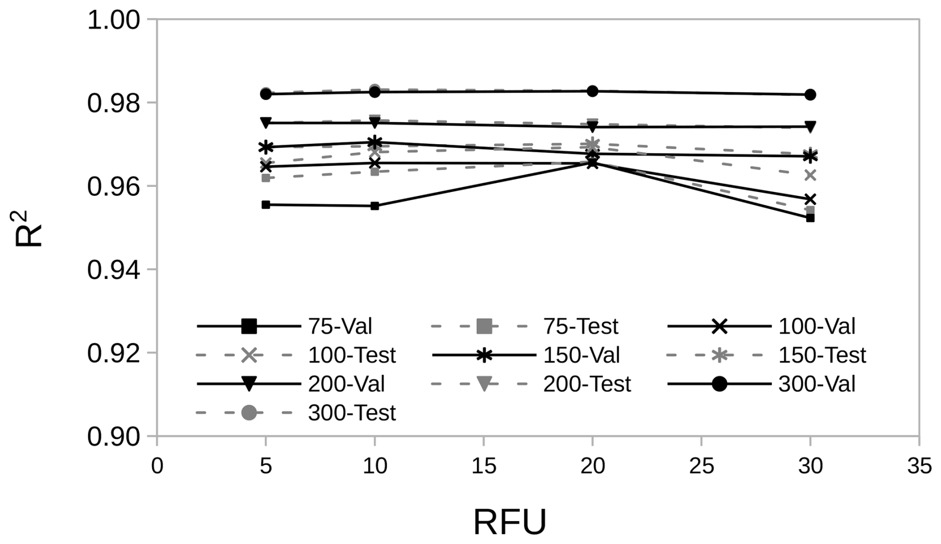
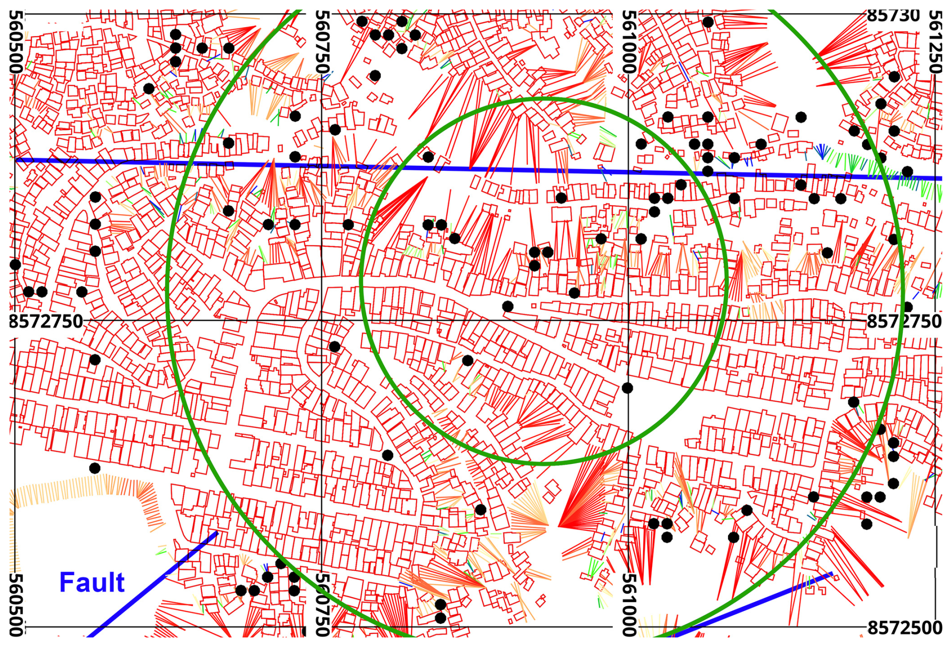
Figure 10 Histograms of the distances between the two nearest centroids of slope areas.

Figure 11 shows the ML performance for a R_i=75 m, T_i=3 d and RFU =20. Although the presence of relatively few scattering points, the ML model presents a similar and excellent performance in both the validation and test phases. In XGBoost, “weight” and “gain” are key concepts related to feature importance and the tree-building process. The weight refers to the number of times a feature is used to split the data across all trees in a given XGBoost model, whereas the gain is linked to the reduction in training loss achieved when using a feature for splitting. The gain quantifies the improvement in the model's performance (reduction in the objective function) achieved by using a particular feature to make splits throughout the ensemble of trees. As observed in Fig. 12a, the variables related to the slope stability analysis, both in natural and saturated states (probability of failure and FoS), and the different periods of cumulative rainfall, had the highest weight values. The density of residences at the slope toe, the quality of the sewage service, and proximity to the rock's faults also had a significant influence on the obtained results, followed by the density of residences at the slope crest. Figure 13 compares the feature's weight for different values of R_i. Although the list of parameters with higher weights remains almost unchanged, the relative weight of the sewage service increases with R_i, going from 14th to 8th place when R_i increases from 75 to 300 m. According to Fig. 12, the input variables for different periods of rainfall presented high values of both weight and gain, meaning that they are often used in splitting data and are effective in improving the model performance. The proximity to the faults in the bedrock, the quality of the sewage service, and the soil permeability tend to form a second tier in terms of variable gain.

Figure 11 ML results for R_i=75 m, RFU =20, and T_i=3 d. (a) validation and (b) test phases.

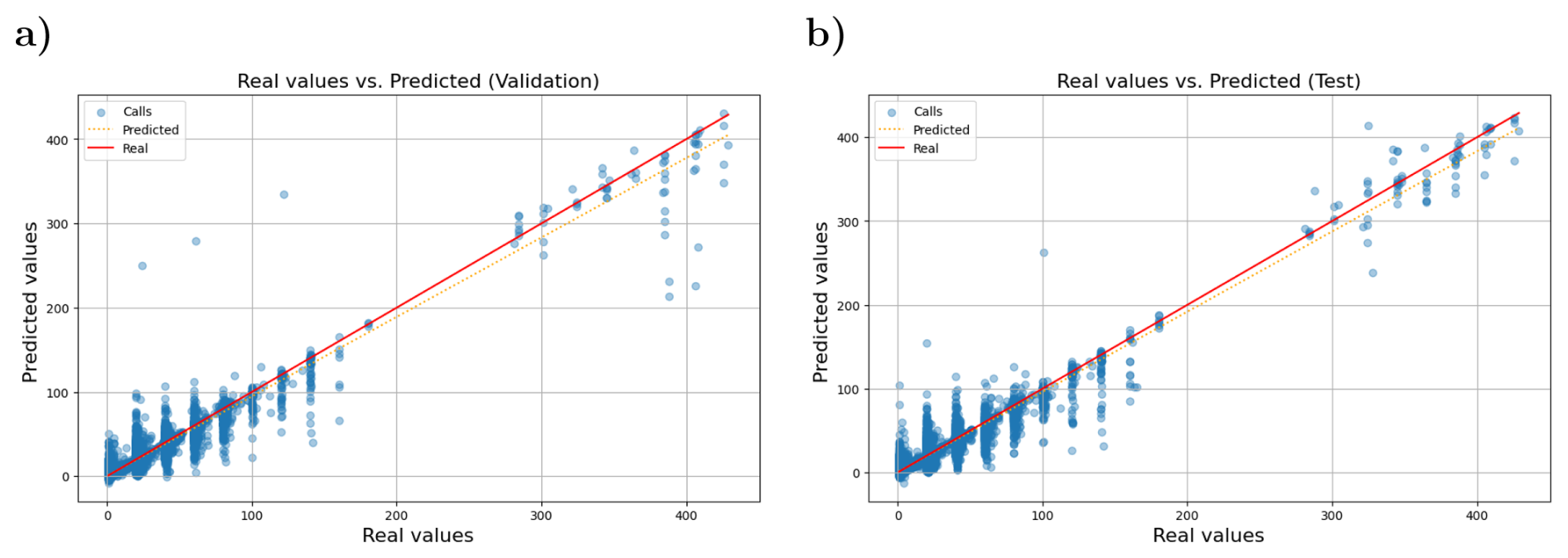
Figure 12 Importance of the features (input parameters) on the ML performance in terms of (a) weight and (b) gain (R_i=75 m, RFU =20, and T_i=3 d).

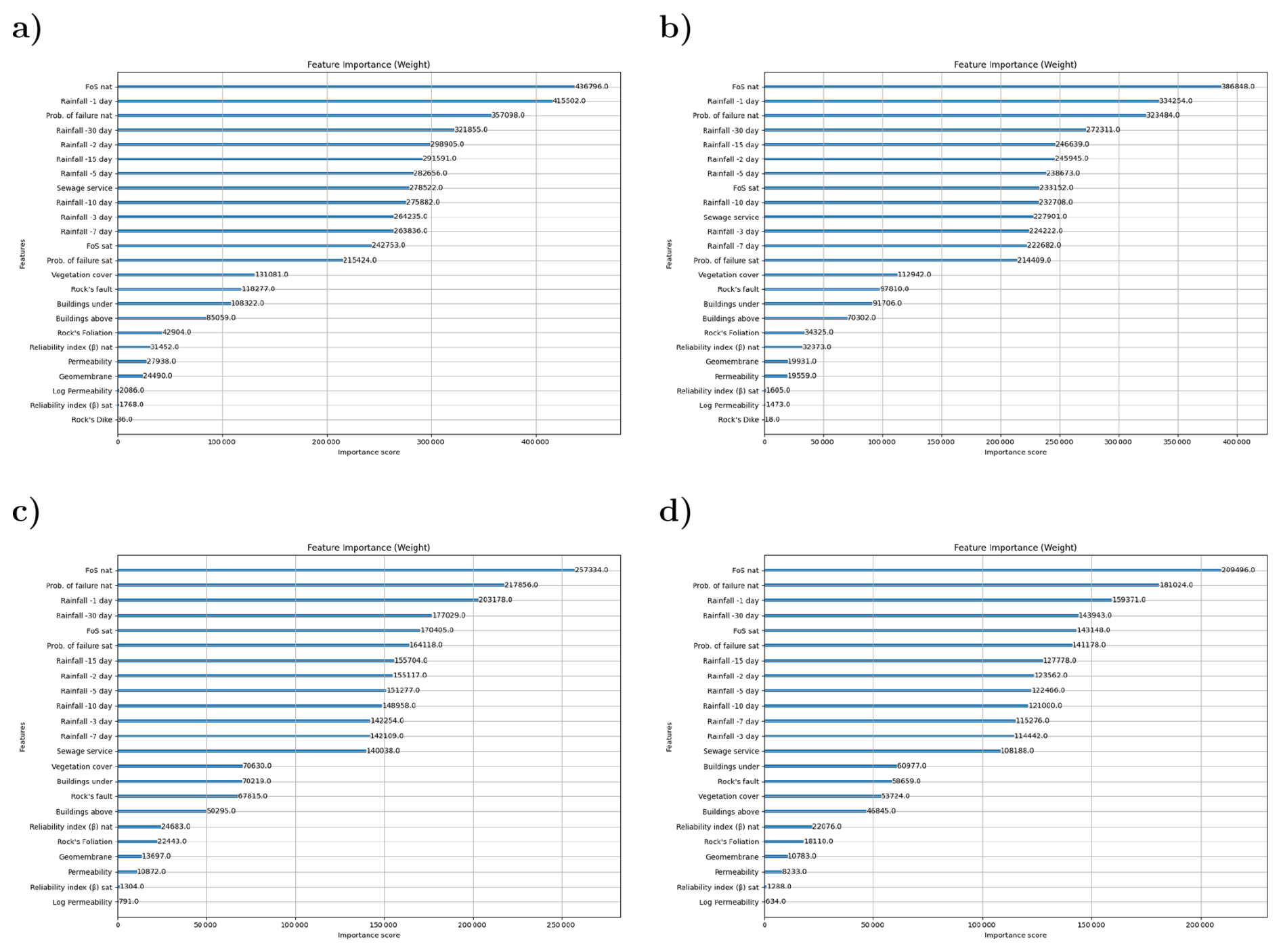
Figure 13 Importance of the features (input parameters) on the ML performance in terms of weight for different R_i values: (a) R_i=300 m; (b) R_i=200 m; (c) R_i=100 m and (d) R_i=75 m. RFU =20, and T_i=4 d.

Figure 14 compares the feature's gain for different values of R_i (RFU =20, and T_i=4 d). The cumulative rainfall inputs still tend to present the highest gains. However, the soil permeability and the faults in the bedrock play a first-level role in this case. The faults in the bedrock lose gain as R_i increases, reaching the 2nd place for R_i=75 m and the fourth position for R_i=100 m. The same pattern is observed for the soil permeability, whereas the quality of the sewage service tends to preserve an intermediate ranking. These findings also suggest that using R_i=75 m is a wise choice because it tends to ensure greater effectiveness for variables other than those linked to rainfall. In gradient boosting, variables that have the highest “weight” (the number of times used in a split) may present smaller “gains” (reductions in loss) in later trees because earlier trees have already captured the most significant predictive power of that feature. Gradient boosting is an iterative process where each new tree is built to correct the errors (residuals) of the previous ones. It must be pointed however, that feature importance metrics based on XGBoost weight and gain should be interpreted with caution in the present study, which involves multiple cumulative rainfall as well FoS, probability, and reliability as model variables, with a clear interdependence relationship, which makes accurately accounting for their individual contribution to model performance much complex.

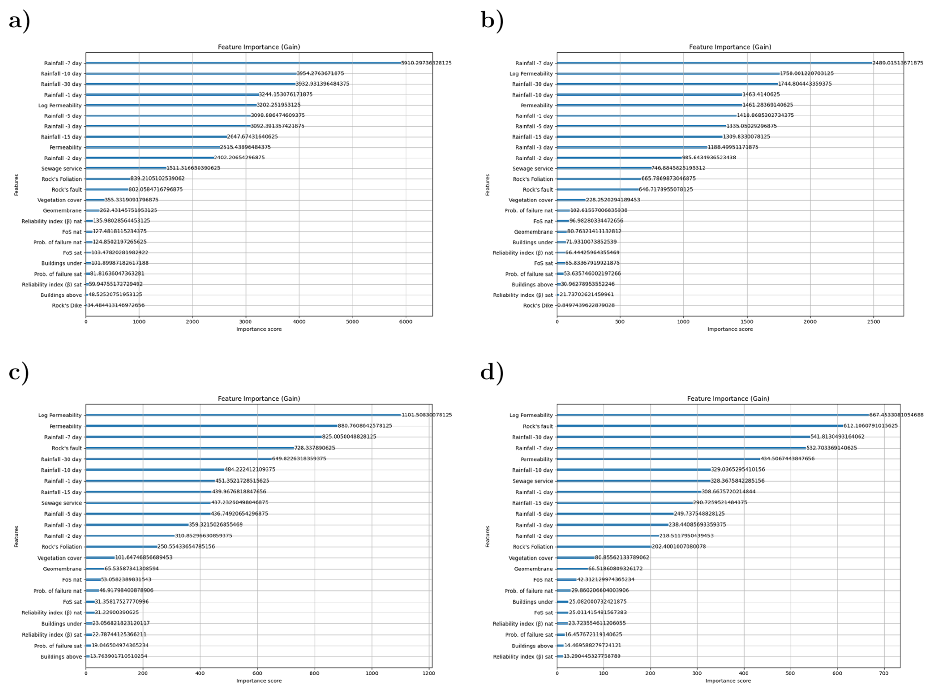
Figure 14 Importance of the features (input parameters) on the ML performance in terms of gain for different R_i values: (a) R_i=300 m; (b) R_i=200 m; (c) R_i=100 m and (d) R_i=75 m. RFU =20, and T_i=4 d.

4 Conclusions

This research paper presents a robust and effective machine learning (ML) framework for the prediction of slope instabilities in the city of Salvador, Bahia, Brazil. The primary purpose was to address the significant challenge of managing slope stability issues in urban areas with complex terrain by developing a data-driven model capable of providing accurate, real-time predictions of soil mass movements. This model was designed to serve as a critical decision-support tool for municipal authorities, enabling proactive risk management so as to ensure public safety. The study's approach involved integrating a comprehensive dataset comprising 13 522 emergency calls (about both confirmed and unconfirmed mass movements) with a digital terrain model (DTM) and extensive geotechnical data. A suite of georeferenced variables was used as input for the ML model, including cumulative rainfall over various time intervals, vegetation cover, key geological structures such as faults and foliations, the status of the sewage collection system, and residential density, both at the slopes's foot and crest. The XGBoost algorithm, a powerful gradient boosting technique, was used to build the predictive model, which was rigorously trained and validated. The results of this study are highly compelling and demonstrate the significant potential of ML in geotechnical hazard prediction. The model achieved an outstanding performance, with an R² value consistently exceeding 0.94 across various scenarios and reaching a peak of approximately 0.98 during both the validation and testing phases. This exceptional accuracy underscores the model's reliability in forecasting slope instability events. A detailed analysis of feature importance revealed that variables directly related to slope stability, such as the Factor of Safety (FoS) and probability of failure, along with cumulative rainfall and the quality of the sewage service, were the most influential predictors. The model's performance was found to be sensitive to parameters like the slope's radius of influence (Ri) and the weighting of confirmed versus unconfirmed emergency calls (RFU), with an Ri of 75 m and an RFU of 20 yielding physically consistent optimal results. The practical implications of this research, particularly for evacuation alarming in high-risk situations, are profound. The high predictive accuracy of the model provides a solid foundation for developing an effective early warning system. By continuously processing real-time data on rainfall and other dynamic factors, the system can identify areas where the risk of slope failure has surpassed critical thresholds. This enables municipal authorities to issue timely and targeted evacuation orders, thereby minimizing the risk to human life and property. The model's ability to be frequently updated with new emergency call data and weather information ensures its dynamic nature, allowing it to adapt to changing conditions and improve its predictive power over time. Ultimately, this work provides a scalable and efficient tool that can be integrated into existing municipal warning systems, transforming reactive responses into proactive risk mitigation strategies and significantly enhancing the resilience of communities vulnerable to slope instability hazards. Although in its present form, the proposed framework demonstrated a strong ability to reproduce retrospective events in time series, this good performance is usually not sufficient to ensure strong predictive performance. Temporal holdout validation and an interactive implementation of this model are under development, aiming to gradually replace the municipality's current warning and emergency declaration criteria. All the new data produced during this period will help with the model implementation task, using walk-forward validation with Sliding Windows to Test Memory Depth, since most variables tend to evolve (e.g., the quality of the sewage collection system and the geometry of the slopes). Different (at least two) thresholds must be defined in this stage, considering the predicted and experimental values of the output variable: a warning and an emergency state. This is a very delicate phase, because declaring an emergency without confirmed events (false alarms) can jeopardize the entire system, leading the population to gradually discredit it and expose them to risk in future events.