Using machine learning for the prediction of flood-related 112 calls

As weather-related disasters become more frequent and severe, there is a growing global push toward impact-based early warning systems, exemplified by initiatives such as EW4All. This transition positions machine learning (ML) and artificial intelligence (AI) as powerful tools for integrating meteorological hazard data with information on vulnerability and exposure into data-driven forecasting systems. In this work, we explore the use of 112 emergency calls as high-resolution impact proxies for an ML-based prediction problem. Specifically, we develop a model that combines rainfall-related weather data, information on recent emergencies, and static vulnerability-exposure layers to predict, at a municipal and hourly resolution, whether flood-related impacts will occur in the next hour. This study covers the period between October 2018 and February 2025 in Catalonia, northeastern Spain.

To address the severe temporal class imbalance and uncertainty characteristics of emergency call data, we define a custom walk-forward evaluation scheme that ensures the same number of positive samples across comparable time periods. We then distribute municipalities into three distinct population density groups (low, medium, and high) and train one model for each one. This stratification enables us to evaluate performance across diverse population dynamics and varying data availability. The resulting models are compared against operational methodologies, such as climatology-based weather warnings issued by meteorological agencies. Our results show that the ML approach represents a substantial improvement in two out of the three groups. The model for the lowest-density group, however, struggles due to a substantial lack of impact data, highlighting a key roadblock for data-driven algorithm development in sparsely populated regions.

Further experiments focus on explainability to improve trust by understanding the models' behaviours using feature importance analyses like SHAP (SHapley Additive exPlanations), feature group selection, and ablation. Additionally, we present a methodology to evaluate model behaviour across different stages of a rainfall event. These experiments show how ML models can effectively combine various data sources to provide more effective predictions than using these sources in isolation. Moreover, while the best-performing model exhibits moderate performance at the onset of rain, it still consistently improves upon traditional baselines. As the event evolves, its prediction skill rises significantly and is maintained even after precipitation has stopped. This highlights the strong potential of even relatively simple ML pipelines to deliver timely, localised anticipation of weather-related impacts.

1 Introduction

Extreme weather and climate events have become a pressing global concern in recent decades, posing significant hazards and leading to major disasters when they intersect with vulnerable populations and natural systems. According to some estimates (United Nations Office for Disaster Risk Reduction, 2015a), natural disasters pose an average annual economic loss of between USD 250 billion and USD 300 billion, with nearly two-thirds of such disasters being caused by extreme weather hazards. Among these events, flooding emerges as one of the main causes of disasters, along with storm surges and windstorms. Flood frequency and intensity are increasing, driven primarily by climate change (Merz et al., 2021), and the growing socio-economic and environmental impacts of floods demand effective risk management strategies to mitigate their consequences.

Traditionally, Disaster Risk Management (DRM) has relied on hazard-centric approaches for the prediction and monitoring of natural disasters by modelling physical weather phenomena (Alfieri and Thielen, 2012; Raynaud et al., 2015; Corral et al., 2019; Park et al., 2019). While effective for understanding meteorological risks, these methods often overlook the socio-economic factors that ultimately determine the real impacts. However, recent trends advocate for a shift toward impact-based forecasting (United Nations Office for Disaster Risk Reduction, 2015b), which aims to anticipate consequences by incorporating data on vulnerability and exposure. This paradigm shift can allow for more targeted decision-making, encouraging proactive responses from all levels of society (Schroeter et al., 2021; Harrison et al., 2022).

The transition toward impact-based forecasting can be understood as a data-integration challenge between very diverse sources. Artificial intelligence (AI) and machine learning (ML) are technologies that excel in processing vast and complex datasets, identifying patterns, and generating useful insights. With this in mind, ML has already proven effective in resource allocation and anticipatory actions (Van Den Homberg et al., 2020; Teklesadik and van den Homberg, 2022), and in weather forecasting (Chen et al., 2023; Nguyen et al., 2024; Alet et al., 2025; Price et al., 2025).

In this work, we propose an ML methodology for predicting flood-related impacts, using emergency calls as the target variable. We focus on Catalonia, in northeastern Spain. The region has a typical Mediterranean climate, resulting in periods of drought and recurring flood events, including intense flash floods. Our methodology works at the municipal level and with hourly temporal resolution between October 2018 and February 2025.

Emergency calls can serve as a very valuable impact indicator, as they represent one of the most immediate signals of population distress, particularly during early stages of flooding. However, it is important to note that the population-dependent nature of these data (they depend on people reporting) makes them heterogeneous both across time (occurring usually during hazardous events) and territory, following the population distribution. From an ML perspective, this results in a highly imbalanced problem, particularly in less populated areas. We address this problem by stratifying models based on population densities, allowing for a better assessment of performance based on the data availability, as this stratification also groups localities with similar urban or rural dynamics.

The main objective of this study is to demonstrate how ML pipelines integrating data on impacts, vulnerability and exposure can produce impact predictions that are more actionable than current operational weather-based systems. We evaluate the methodology's capacity to increase detection power and reduce false alarms when compared to hazard-based baselines (e.g., official weather warnings) across different population densities. Furthermore, we analyse how performance depends on data availability, highlighting the main limitations of impact modelling in less populated regions.

2 Related work

Impact and risk assessment for floods has traditionally been approached by combining hazard-based models with static layers of vulnerability and exposure. An example in flash floods is the ReAFFIRM method (Real-time Assessment of Flash Flood Impacts; Ritter et al., 2020), which quantifies impacts on population, economic losses, and affected critical infrastructure. This methodology was later expanded to the pan-European level in ReAFFINE (Real-time Assessment of Flash Flood Impacts at paN-European scale; Ritter et al., 2021). For pluvial floods, Meléndez-Landaverde and Sempere-Torres (2025) introduced a site-specific framework (SS-EWS) to guide the design of community-based, impact-focused early warning systems. Furthermore, Láng-Ritter et al. (2022) developed a methodology for forecasting the impacts of compound floods by leveraging predictions from both fluvial and flash flood models. The European Flood Awareness System (EFAS; Thielen et al., 2009, European Commission, 2026) currently integrates operational products developed under the TAMIR project (Advanced Tools for pro-Active Management of Impacts and Risks Induced by Convective Weather, Heavy Rain and Flash floods in Europe; Niemi et al., 2021); and it is planned to incorporate tools from EDERA (Early warning Demonstration of pan-European rainfall-induced impact forecasts; Berenguer et al., 2024; EDERA Consortium, 2025), the successor to TAMIR. Together, these systems can enhance the anticipation and management of the risks posed by heavy-rainfall-induced events across Europe.

Although less common than physical methods, machine learning (ML) methodologies are increasingly being explored for impact assessment. In flood risk management, AI approaches enable automated mapping and dynamic inundation forecasting, which are critical for real-time warnings and resilience planning in vulnerable urban areas (Zhou, 2025). For instance, Terti et al. (2019) explored the probabilistic prediction of flash-flood-related human incidents and fatalities using random forest classifiers. Moving to the topic of tropical cyclones, an early example of ML-based impact forecasting was developed by the 510 initiative of the Netherlands Red Cross to predict the humanitarian impact of typhoons (Wagenaar et al., 2021; Teklesadik and van den Homberg, 2022), classifying municipalities based on whether more than 10 % of houses were completely destroyed or not. This approach was later improved by Kooshki Forooshani et al. (2024), adapting the methodology to work with globally available data. Additionally, Zheng et al. (2025) developed a multi-hazard impact modelling framework for economic loss assessment. Moreover, some works have also seen success in modeling weather-related impacts on airport disruptions (Schultz et al., 2021; Dalmau et al., 2023). The application of ML tools in the context of disaster risk reduction is promising. However, as highlighted by Kox et al. (2025), these systems should not replace human decision-making, but rather serve as decision support tools that must be implemented ethically and responsibly. Consequently, explainable AI (XAI) techniques are increasingly used to improve the trust and transparency of these models, mitigating the “black-box” problem and helping to understand the links between hazards and susceptibility (Alcântara et al., 2025). Techniques like SHAP (Lundberg and Lee, 2017) and LIME (Ribeiro et al., 2016) are commonly paired with machine learning approaches to identify key predictors and provide interpretability. For example, in hurricane risk assessment, Gao and Wang (2023) employed LIME alongside deep learning methodologies to offer actionable knowledge to stakeholders, improving proactive risk mitigation.

To train such impact models requires robust and comprehensive datasets. Emergency calls, as high-resolution indicators of population distress, serve as an excellent proxy for real-time impacts and have been used in the past to approximate weather damage. Early studies, such as Schuster et al. (2005), used calls to correlate hailstone size with on-the-ground damage in Australia. Rossi et al. (2013) use emergency calls in the context of convective storms, introducing a methodology capable of tracking the storm path and determining the hazard level. More recently, several case studies have demonstrated the value of calls for refining flood risk mapping and creating impact catalogues (Camarasa-Belmonte and López, 2018; Oliva and Olcina, 2022; Ortiz et al., 2024). The utility of these types of data have also been proven for relating the impact of rainfall on road accidents through ambulance dispatches (Sangkharat et al., 2021), and for developing a framework for exploring urban vulnerability dynamics through ambulance calls (Sirenko et al., 2025). However, access to emergency call data, and impact data in general, is severely limited. To address this gap, Gaztelumendi et al. (2024) presented a comprehensive methodology for building such catalogues, including emergency calls. The framework was later operationalised by the Basque Meteorological Agency. But even when available, impact data tend to be sparsely distributed both temporally and spatially due to the infrequent nature of impactful weather events, but also underlying socio-economical characteristics (Diboulo et al., 2012; Brousse et al., 2024). The study conducted by Papagiannaki et al. (2026) shows how impacts are predominantly concentrated in major urban areas, suggesting that population density and regional characteristics influence recorded incidences. To account for this, we explore a methodology for training distinct models based on population density.

Closest to our work is the study by Iglesias et al. (2024), which also employs ML and emergency call data in Catalonia to make predictions at the municipality level, with great success compared to traditional daily meteorological warnings. However, their model targets multiple weather phenomena simultaneously and operates at a daily resolution, potentially missing fast-occurring events such as flash floods, which require finer temporal resolutions (Collier, 2007) and are particularly common in the region, often resulting in significant losses (Barnolas and Llasat, 2007). Our work aims to advance this line of research by producing hourly predictions focused specifically on flood-related impacts, offering more granular and timely information for emergency response.

3 Study region

This section describes the study area, focusing on its geographical and climatological characteristics and the distribution of its population. The chosen spatial and temporal resolutions for the study are also presented.

3.1 Geography and climate

This study is centred around Catalonia, located in northeastern Spain. Its territory has a surface area of approximately 32 000 km², and borders Andorra and France to the north, with the Valencian and Aragonese autonomous communities to the west and south, respectively, and with the Mediterranean Sea across all the eastern border.

Catalonia has a typical Mediterranean climate. Winters are mild and summers are hot and humid (mean yearly humidity is around 70 % to 75 %), and the significant variation in topography gives rise to a variety of climates. It receives ∼ 700 mm of annual rainfall with irregular interannual distribution. Flood events are recurring, including intense flash floods. The main causes for this are the evaporative nature of the Mediterranean Sea and the “Litoral” and “Prelitoral” mountain ranges, which run parallel to the coast, acting as natural barriers and forcing hot, humid masses of air to quickly rise, cool, and condense. On the other hand, in the territories surrounding the Pyrenees, longer and less intense rain episodes are most common. Despite all this, Catalonia is also prone to periods of drought. Most notably, water reserves reached historical lows during the drought episodes of 2023 (Cascante, 2023).

3.2 Population

In total, 8 012 231 inhabitants live in Catalonia (Statistical Institute of Catalonia, 2024), distributed across 947 municipalities. Approximately two-thirds of the total (5 066 684 inhabitants) live inside the Barcelona Metropolitan Demarcation, one of nine vegueries (a high-level regional division). The second and third most populated ones are the Girona region with 804 851, and Camp de Tarragona with 555 957. This highlights how Catalonia's population is heavily concentrated around major coastal cities, and particularly around the Barcelona area, while the rest of the territory is sparsely populated. This distribution can be clearly seen not only in terms of absolute population values, but also when looking at population centres (Fig. 1).

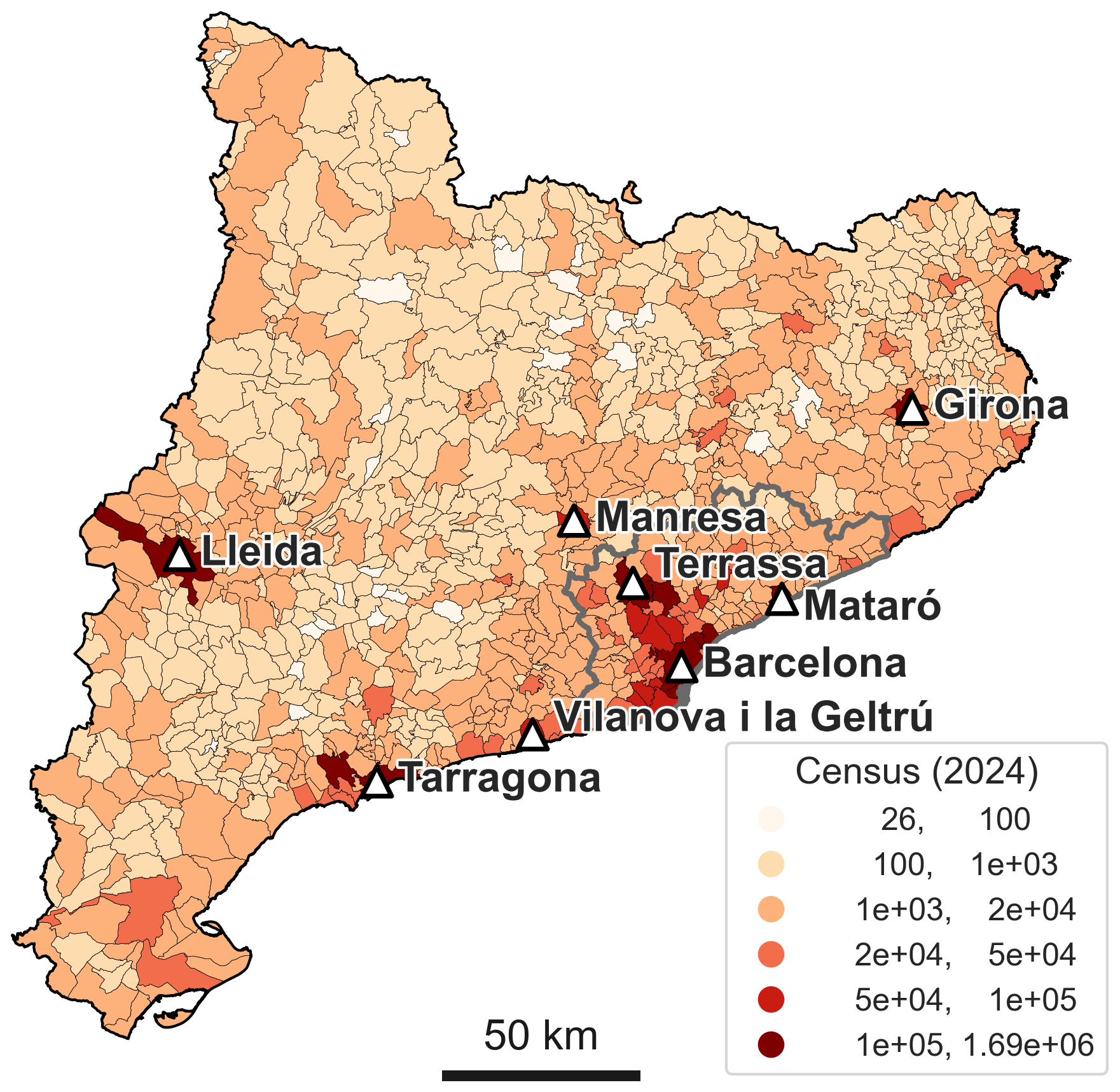
Figure 1 Catalonia's population distribution by municipality. Additionally, we highlight important city centres. Note how the population is heavily skewed towards the coast, and especially around the city of Barcelona (Barcelona Metropolitan Demarcation, in grey).

These significant population disparities across Catalonia create two important challenges. First, the class imbalance becomes even more severe in less populated municipalities, with the great majority of calls being concentrated in the most populated areas. Secondly, urban and rural areas often react differently to severe weather events, a pattern reflected in Fig. 2 as the positive correlation between the total number of emergency calls and municipal population.

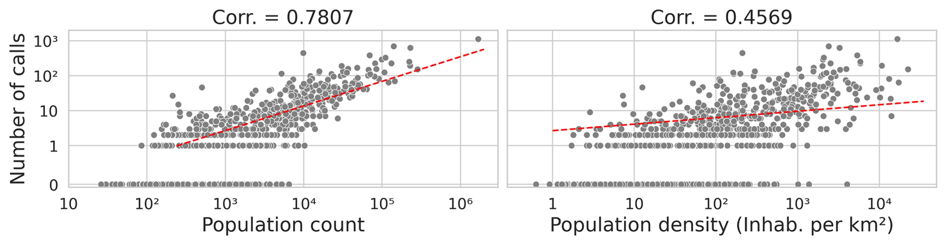
Figure 2 Relationship between total emergency calls and municipality population (left) and density (right). Each point represents one of the 947 municipalities in Catalonia. The correlation coefficients and their corresponding linear fits (red dashed line) are indicated. Note that all axes are in logarithmic scale (except for values between 0 and 1, for which a linear scale is used). The linear regression was fitted using the logarithms of the variables, ignoring instances without calls (where the log is undefined).

To mitigate these issues, we divide the territory into three equal-sized population density groups and train individual models for each. We group by population density rather than by census, as density has a more direct relation to the notions of “rural” or “urban”. Figure 3 shows the result of this grouping. High-density municipalities are mostly clustered along the coast, primarily in the central area around Barcelona. Medium-density towns tend to be adjacent to high-density ones, while low-density municipalities fill the gaps between major populated areas in the interior and along the Pyrenees.

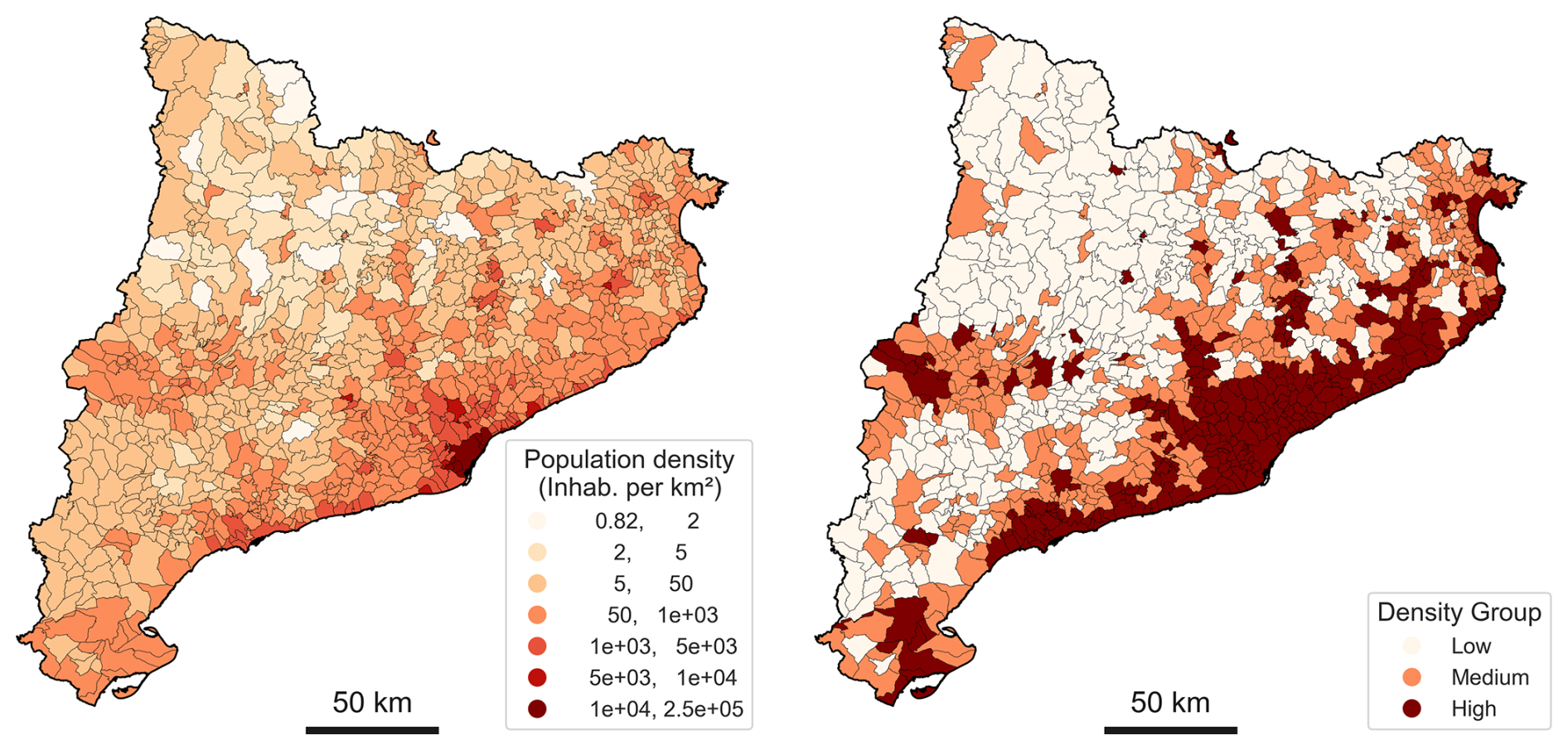
Figure 3 Population density per municipality (left) and the resulting density-based groups (right). Municipalities are classified into three groups of equal size (316, except Medium with 315), using the following population density thresholds (inhabitants per square kilometre): [0,20) for the Low Density group; [20,120) for Medium Density; and [120,∞) for High Density.

3.3 Study resolution

The study covers a time window of nearly six and a half years, from 27 October 2018 to 28 February 2025. There is a gap in the data from 14 March to 31 December (both included) of 2020, first due to the COVID-19 confinement (a period which we ignore because impact data potentially exhibited a different behaviour), and a later, unrelated, gap of missing data in our dataset

From our conversations with Catalonia's Civil Protection, we derive the municipality as the basic territorial unit used when coordinating emergencies (General Directorate of Catalonia Civil Protection, 2022). Based on this, we choose to also use the municipality as the spatial unit of this work. In particular, we employ the municipality boundaries found in Cartographic and Geological Institute of Catalonia (ICGC) (2024), with a territorial detail scale of 1:5000. Regarding temporal resolution, we will work at an hourly resolution, making predictions at the start of every hour, and with a forecast horizon of one hour.

4 Data

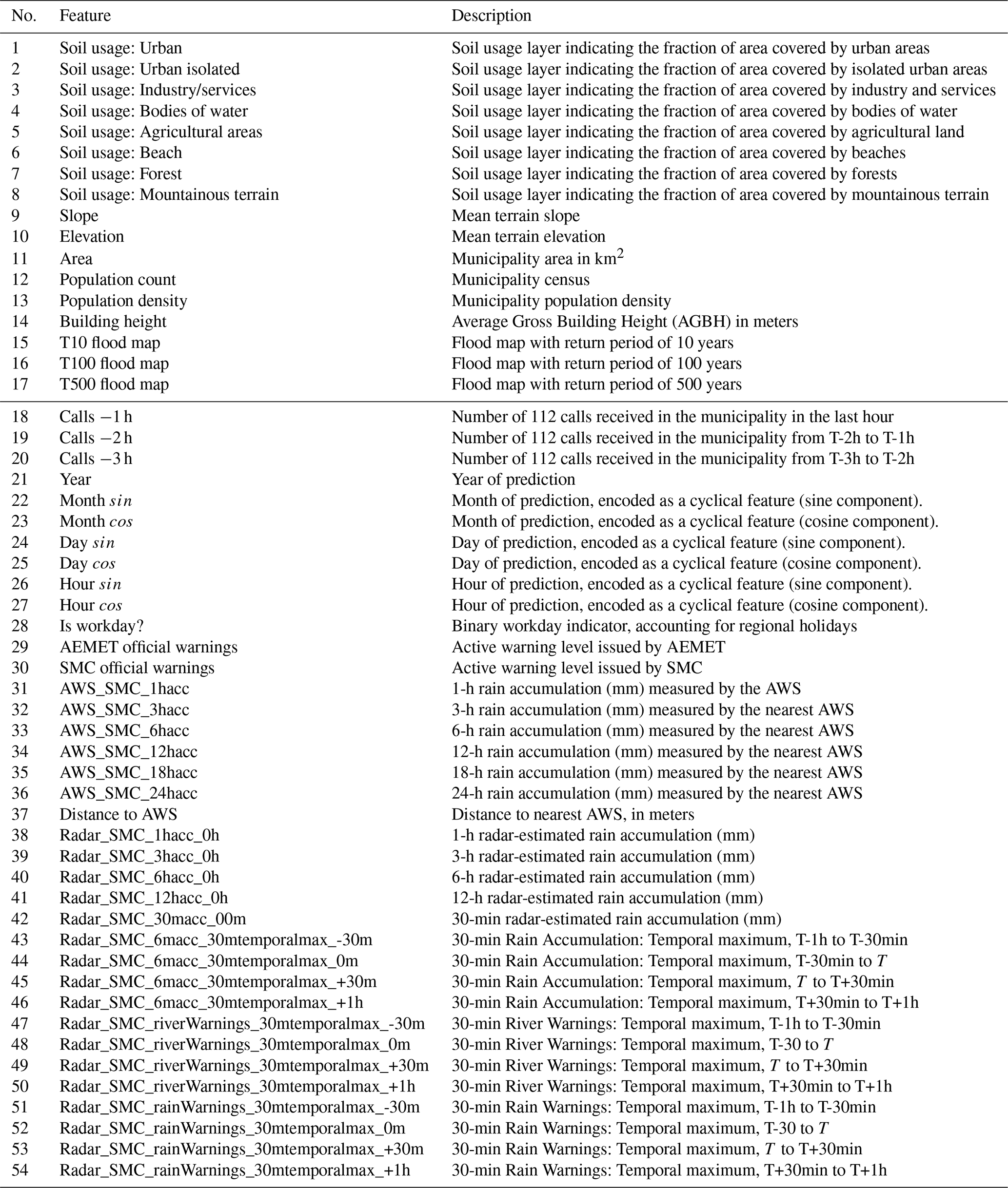
To successfully model impact, it is essential to provide relevant and diverse information so the model can identify relationships between input data and the ultimate impacts. This section describes how our dataset is created, including the integration of static and dynamic data sources at the study's resolution and the partitioning of the data based on population density groups. In the end, 54 input features are created (see Table A1 for the full listing).

4.1 Target data

This work trains machine learning (ML) models to predict flood-related emergency calls to 112, the European emergency number, a powerful indicator of severe weather consequences on the population. We design this as a binary classification task: for each municipality and timestamp, the model predicts whether one or more such calls will occur within the next hour. The data used for this study were provided by the Catalan Civil Protection authorities.

The data contain information about the position (longitude-latitude), time, and categorization of individual calls based on the type of emergency. To ensure precise labelling for model training, only calls explicitly categorised as “flood” or “flash flood” have been included in the study. This was necessary because, while other categories are also potentially related to floods (e.g., traffic incident, power outage), these relationships are weaker. Note, however, that there is no guarantee that there is really causality, only coincidence with a flood or heavy rain event.

The final selection of calls is aggregated to the study resolution to obtain the number of calls per municipality and hour. Since we are modelling a binary problem, an impact threshold must be defined to create a Boolean target (i.e., where the number of calls is greater than or equal to the impact threshold). We use a threshold of 1 call per hour for the medium- and low-density groups, as selecting a higher threshold would excessively reduce the already limited number of impacts. For high-density municipalities, we experimented with different thresholds and found that values varying between 1 and 5 yielded similar results. Ultimately, we opted for 3 calls, as it resulted in a number of impacts comparable to that of the medium-density group. Instances meeting these respective thresholds constitute the positive class, while all other samples form the negative class, which signifies no-impact.

Table 1 shows the number of calls for each population group, as well as the final target after applying the impact threshold. The values presented here reflect the data after applying the daily rainfall filter presented in Sect. 4.4, which significantly reduced the number of negative samples. Low-density municipalities recorded only 279 calls during the entire study period, compared to the 11 736 in high-density areas. This disparity is also reflected in the number of impacts, although the difference between Medium and High is less pronounced due to the more severe threshold applied. It is also interesting to note a notable shift in call type distribution: flash flood-related emergencies appear to decrease as population density increases (19.35 %, 12.69 %, and 6.35 % for Low, Medium, and High density groups, respectively), signalling that rural areas might be less resilient to these kinds of events. In all cases, an extreme class imbalance is present across all population groups, as indicated by the low positive rate (i.e., the fraction of total samples belonging to the positive class).

Table 1 Emergency call statistics and target distribution across population density groups. Specifically, the table presents the total number of emergency calls, their categorization into flood or flash flood events, and how they translate into final positive samples based on the study's resolution. The presented statistic were obtained from the dataset after applying the daily rain filter detailed in Sect. 4.4.

Finally, Fig. 4a shows the geographical distribution of calls. As population density decreases, a growing number of municipalities have received only a few calls, or none at all. Even within high-density municipalities, a significant disparity exists between major cities like Barcelona, Terrassa, and Tarragona, which show the highest values (red), while the rest have generally registered between 10 and 100 calls. The distribution of the number of calls for the Low and Medium groups is very similar to that of the number of positive instances (see Fig. 4b), as in these municipalities it is uncommon to register more than one call per hour. However, for the high-density group, the use of a higher impact threshold means that many instances with fewer than 3 calls per hour are filtered out, giving rise to a more concentrated pattern of significant impacts.

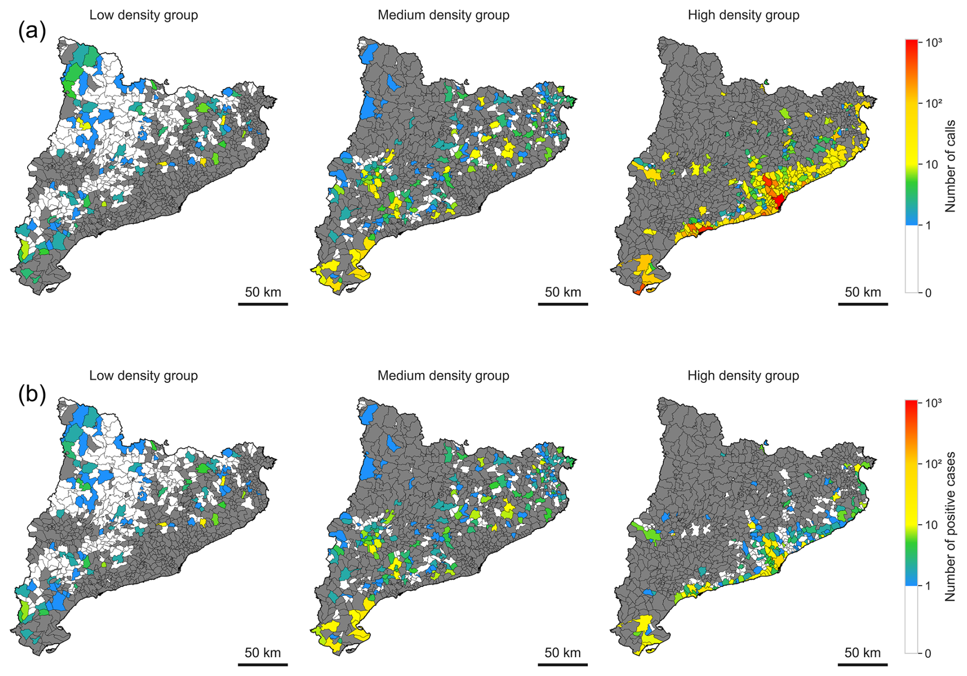
Figure 4 Number of calls and positive instances received per municipality over the duration of this study. Municipalities belonging to other groups are shown in grey.

4.2 Static input data

Static data refers to data that do not vary over time and is instead used to represent population dynamics and characteristics. In particular, the following data are collected:

1. Population census (National Institute of Statistics, 2024), from which we also derive the population density for each municipality (inhabitants per square kilometre).

2. Multiple soil usage layers (eight features in total: Urban , Urban Isolated, Industry and Services, Bodies of Water, Agricultural Areas, Forests, Mountainous Terrain, and Beaches). These layers are formed by grouping different categories from the original Soil Usage raster in Cartographic and Geological Institute of Catalonia (ICGC) (2022) and are projected to the municipality level by taking the fraction of the municipality's area covered by each layer.

3. Flood maps (three features with return periods of 10, 100, and 500 years), provided by the Ministry for Ecological Transition and the Demographic Challenge (2024), aligning with the goals of the INSPIRE European Directive (European Parliament and Council of the European Union, 2007). Each flood map is converted to the municipality level by computing, for each municipality, the fraction of the municipality's area covered by the flood map.

4. Topographical data (two features). In particular, we take the mean slope and elevation for each municipality. For the elevation, we use data from the EuroDEM digital elevation model (Eurogeographics, 2024). For the slope, we use the slope layer of the CatLC dataset (Cartographic and Geological Institute of Catalonia (ICGC), 2021a, b, 2025).

5. Average building height in each municipality. We use the Built-H spatial raster found in the Global Human Settlement Layer data package (GHS-BUILT-H; Pesaresi and Politis, 2018; Pesaresi et al., 2024)

4.3 Dynamic input data

Capturing adequate hazard information is a crucial step in the forecasting of flood impacts. In this section, the dynamic data sources (i.e., data that vary over time) used to train our models are described, providing crucial hydrometeorological information about hazards.

4.3.1 Automatic weather station data

One of the data sources used for this work is the historical measurements provided by SMC's network of automatic weather stations (AWSs), which are publicly available online through SMC's REST API (Meteorological Service of Catalonia (SMC), 2023).

For the scope of this project, we retrieve data from the 30-min rain accumulation variables. We then create larger accumulation intervals to serve as inputs for our models, capturing the temporal evolution of the rain. In the end, we derive six features for 1-, 3-, 6-, 12-, 18-, and 24-h rainfall accumulation. These features are created at the start of every hour, and projected to the municipality level by taking, for each municipality, the value of the closest AWS. Distances are computed as the Euclidean distance between the AWS coordinates and the centroid of the polygon defining each municipality. This distance is also provided to the model as an additional feature.

4.3.2 Official weather warnings

Official weather warnings refer to those warnings issued by meteorology agencies to inform about meteorological hazards that could potentially pose a risk to activities, people, and infrastructure. In our research, we collect official warnings issued by both AEMET, the Spanish State Meteorological Agency, and the SMC, the Meteorological Service of Catalonia. Below, we explain the particularities of each one:

• AEMET warnings: AEMET warnings, which contribute to the European MeteoAlarm project (EUMETNET, 2025), were obtained through AEMET's OpenData API (Spanish National Meteorological Agency (AEMET), 2016). These warnings are issued for specific isoclimatic zones, which represent regions with similar climatic characteristics. In the case of Catalonia, after ignoring 5 regions that cover the sea, 16 warning zones can be found. Only the warning categories of “Storm”, “1 h Rain Accumulation” and “12 h Rain Accumulation” are considered as hazards. Each warning has one of three possible severity levels, from least to most severe hazard: “yellow”, “orange” and “red”. “Green” is used when there is no warning. We convert these levels to numerical values (0 for “green”, up to 3 for “red”).

• SMC warnings: These warnings are publicly available using SMC's REST API (Meteorological Service of Catalonia (SMC), 2023). They are issued at the comarca (county) level. As of February 2025, there are 43 of these regions, but this number has been changing in recent years, with the last modification being the creation of the Lluçanès county in 2023. This does not impact our data as municipality boundaries are not affected. We use the adequate administrative boundaries depending on the warning's date to assign the right warning level to each municipality. Only “Rain intensity” and “Rain accumulation” warnings are taken into account. SMC uses a hazard level taking values from 1 to 6, from lowest to highest hazard degree.

  SMC also issues “observation” warnings to emphasise a significant meteorological event in an already-warned region, or to update regions where a significant event has been observed that previously had not been warned. For our analysis, all warnings are used, and only the most recent warning level for each municipality and time step is used.

In the end, SMC and AEMET warnings are treated as two different features, translating each to the municipal level by taking the maximum warning level active for each municipality and hour (Fig. 5).

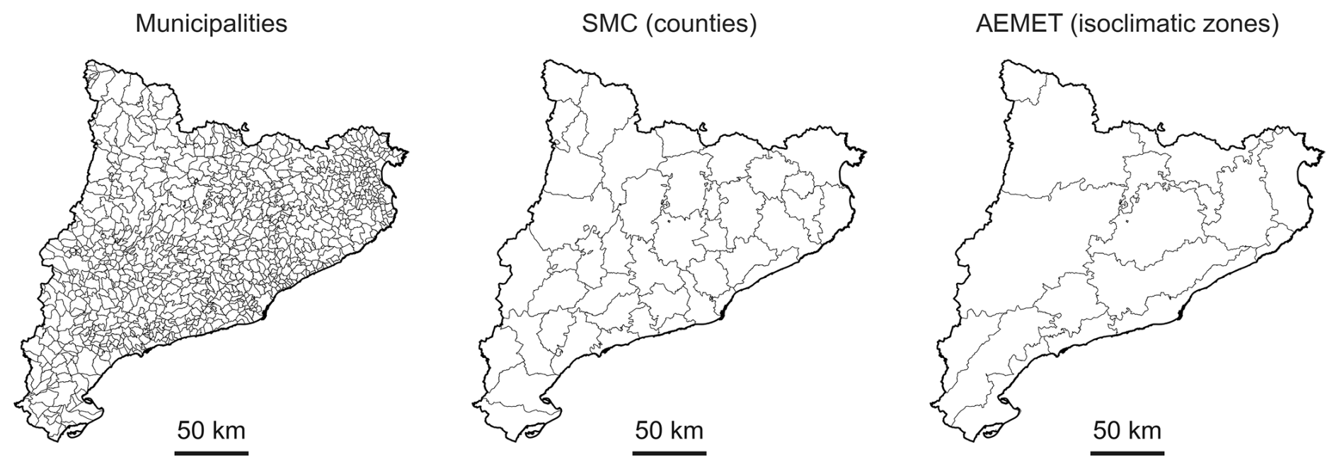
Figure 5 Spatial resolution of SMC (middle) and AEMET (right) warning zones compared to the study's municipality-level resolution (left). For this work, warnings are translated to the municipality level by taking the maximum active warning level for each one.

4.3.3 Radar data

Weather radars are remote sensing tools used to detect rain presence and estimate its intensity. The SMC has a network of 4 C-band Doppler radars, which scan the sky at multiple elevation angles and produce volumetric observations every 6 min. These observations are processed to estimate the precipitation on the terrain, producing precipitation observation rasters at a 1 km resolution. We aggregate multiple of these rasters to create larger rain accumulation periods of 30 min and 1, 3, 6, and 12 h. Moreover, we create a temporal maximum for the most recent two half-hour periods by calculating the pixel-wise maximum from the last ten 6-min rainfall rasters.

Additionally, we utilise two products derived from the radar data (Corral et al., 2019; Park et al., 2019):

• Rain warnings: A statistical estimation of rainfall intensity, expressed in terms of its return period (in years) to quantify the rarity of the event for each pixel.

• River warnings: A statistical estimation of the basin-aggregated rainfall intensity that accounts for upstream contributions in the drainage network. Similarly to Rain Warnings, these values are expressed as return periods (in years).

These products are obtained every 6 min and aggregated using the same temporal maximum procedure as the 6-min rain accumulation rasters.

To provide our models with some prediction data for the next hour, we use radar nowcasting (Berenguer et al., 2005, 2011) to obtain a forecast of the 6-min rain accumulation rasters for the next hour, which is also used to obtain predictions of the River and Rain warning products. Temporal maxima are again used to aggregate these forecasted rasters for the upcoming two half-hour periods.

Finally, the different radar products are projected into the municipality domain by taking the maximum value for each municipality and hour of the dataset. We choose the maximum to not “dilute” essential information about maximums.

4.3.4 Number of calls in past hours

We also create three additional features with the number of flood-related emergency calls received 1, 2, and 3 h ago. These features incorporate some auto-regressive behaviour into the model.

4.3.5 Date features

Date features are derived from the date of each sample. “Year” is a simple integer feature, while “Month”, “Day”, and “Hour” are encoded as cyclical variables (with periods 12, the number of days in the given month, and 24, respectively) following Eq. (1), where v is the variable's value, and T its period. This results in two features for each cyclical variable (7 input features in total, counting the singular year feature).

$$\begin{array}{}\text{(1)}& f_{\mathrm{1}}=\text{sin}\left({\displaystyle \frac{v\mathrm{2}\mathit{\pi }}{T}}\right);f_{\mathrm{2}}=\text{cos}\left({\displaystyle \frac{v\mathrm{2}\mathit{\pi }}{T}}\right)\end{array}$$

4.4 Daily rain filter

The exceptional nature of emergency calls creates an extremely imbalanced dataset, as positive impact cases are very rare. This is further exacerbated by Catalonia's drought periods, resulting in many days with no useful signal for modelling flood impacts.

To mitigate this, we apply a retrospective daily filter to include in the dataset only days with significant observed rainfall. A day is included if at least three automatic weather stations register a 30-min rain accumulation exceeding a set threshold. After evaluating several thresholds, we selected 3 mm as it optimally balances data reduction with call retention, removing 1603 potentially uninformative days (only 245 calls occurred) while preserving 15 081 calls across 714 relevant days.

Regarding the operational validity of applying this filter, the models developed in this study could still be deployed every hour. Even after removing a significant number of days without rainfall, samples where neither rainfall nor impacts occurred still constitute the majority of the dataset, allowing models to train on situations without risk. The objective of the filter is just to mitigate class imbalance by focusing the problem towards days with actual impact potential. Therefore, please note that the metrics presented in the following sections reflect performance strictly under these conditions rather than over a continuous operational deployment.

5 Methodology

In this section, we describe the methodology followed in the study. This includes the definition of the baselines, relevant metrics, and the evaluation setup.

5.1 Model choice

For this work, we base our approach on eXtreme Gradient Boosting (XGBoost; Chen and Guestrin, 2016) classification model, a robust and fast traditional machine learning method well-suited for tabular data and unbalanced learning problems. We also tested other methods such as Random Forests, AdaBoost, and logistic regression, but no significant improvements were observed.

5.2 Baselines

Given that there are no previous works on the classification task approached in this paper with a similar resolution, we compare our approaches against official weather warnings, as they serve as the standard for communicating hazardous weather phenomena to society. We use the same weather warnings described in Sect. 4.3.2, considering only rainfall-related warnings. Additionally, we define a baseline using the River Warnings radar product (Sect. 4.3.3, referred to as FF-EWS from now on), as Civil Protection agents have also found it to provide good results and utilise it operationally.

Importantly, all these baselines are meteorology-based and do not use any information on vulnerability and exposure for their calibration and threshold definition.

Three random baselines were also tested: always predicting negative, always predicting positive, and a stratified approach that predicts the positive class with the same probability as its frequency in the dataset. All three obtained nearly 0 % across all metrics and population groups.

5.3 Evaluation setup

To evaluate the performance, we use the Critical Success Index (CSI; Eq. 2) as the main metric, commonly used in meteorology and forecast verification (Stanski et al., 1989), measuring the fraction of correctly predicted positive cases while penalizing for both false positives and false negatives. Additionally, we provide the recall (the fraction of total observed positive cases that were correctly predicted; Eq. 3) and the precision (the fraction of positive predictions that corresponded to actual impacts; Eq. 4) for a more comprehensive assessment.

$$\begin{array}{}\text{(2)}& \begin{array}{rl}& \text{Critical Success Index}=\\ & {\displaystyle \frac{\text{True Positives}}{\text{True Positives + False Negatives + False Positives}}}\end{array}\end{array}$$

$$\begin{array}{}\text{(3)}& {\displaystyle }& {\displaystyle }\text{Recall}={\displaystyle \frac{\text{True Positives}}{\text{True Positives + False Negatives}}}\text{(4)}& {\displaystyle }& {\displaystyle }\text{Precision}={\displaystyle \frac{\text{True Positives}}{\text{True Positives + False Positives}}}\end{array}$$

Due to the temporal nature of the data, we employ a walk-forward validation scheme, training ten distinct models that sequentially advance in time (Fig. 6). Each model is trained on all available past data and evaluated on dedicated validation and test sets. In particular, the first model is trained on data preceding 1 January 2021.

Figure 6 Walk-forward evaluation scheme used in this study. Models are trained on ten temporal configurations, each advancing further in time than the previous. Validation and test sets are built ensuring they contain the same number of positive examples, not only between themselves but also across all configurations. To assess the variability of the test result metrics, bootstrapping is used to generate 250 random samples, evaluate them, and estimate their variance.

To mitigate the high temporal variability in impact occurrence, we construct 10 validation and test sets to contain the same number of positive samples, preventing periods with few impacts from skewing the metrics. This alone results in sets with significant size disparities. To homogenise set sizes and increase temporal coverage, we also allowed for overlap between validation and test sets from different temporal configurations. Further details regarding the timelines for all temporal configurations across the different population groups are presented in Appendix D.

The validation set results are used for two purposes:

1. Hyperparameter optimization: For the machine learning models, we use the Optuna framework¹ (Akiba et al., 2019) to maximising the Area Under the Precision-Recall Curve (AUC-PR). This step is not applied to the baselines.

2. Threshold selection: We select the optimal classification threshold by maximising the CSI on the validation set. For the baseline methods, we instead select the most effective warning level (or return period for the FF-EWS approach) to be used as an activation threshold. The concrete classification and activation thresholds chosen can be seen in Appendix C.

The final performance metrics are reported on the test set. We compute the mean and standard deviation across all ten configurations to estimate the overall performance of each approach. Given the observed temporal variance during experimentation, we also provide the metrics for each individual configuration and its estimated uncertainty through bootstrapping. Specifically, we follow a 1-d block bootstrap strategy on the test set to generate 250 random samples with replacement, compute performance metrics for each, and take the standard deviation as a measure of uncertainty. To maintain a consistent positive-to-negative class balance across resamples, we fixed the number of sampled “positive days” (i.e., days containing at least one positive instance). We opted for a block bootstrap to account for the temporal correlation between observations belonging to the same rainfall event, using 1-d blocks since the majority of rainfall events in the region last no longer than one day.

While we acknowledge that the validation scheme proposed can lead to different test periods, background distributions, or varying numbers of negative samples, after extensive experimentation with multiple approaches, we have found that stabilizing the positive class was the most effective way to derive meaningful insights from such an imbalanced dataset. Other strategies, like fixing temporal periods (e.g., specific months), resulted in highly inconsistent counts of both positive and negative samples per set, leading to high variance in performance metrics. Conversely, fixing the total number of samples led to sets with drastically different positive-to-negative ratios and varying temporal periods. Furthermore, under both previous approaches, we could not ensure that the validation and test sets contained any positive samples, an issue especially common in medium- and low-density municipalities.

5.4 Class imbalance

As mentioned in Sect. 4.1, class imbalance is a major concern across all population groups. To mitigate this issue, we apply class weighting to the loss function during model training, imposing a higher penalty for misclassifying the impacts (which are the minority class). Specifically, positive instances are assigned a weight inversely proportional to their overall frequency within the training set.

6 Results

Table 2 shows the mean and standard deviation of test set results. Performance improves drastically with population density. In particular, regarding the Critical Success Index (CSI), while the low-density model struggles to surpass 1 % (0.83 %), medium- (9.52 %) and high-density (28.77 %) models achieve more competitive results. This is also true for the precision and recall metrics. It is worth mentioning that these results are obtained using the group-specific impact thresholds from Sect. 4.1, so population density is not the only factor influencing performance. However, because the low- and medium-density groups both share the same impact threshold of 1 call, the superior results of the medium-density model confirm the underlying effect of population density.

Table 2 Mean (± standard deviation) test results for the three population group models.

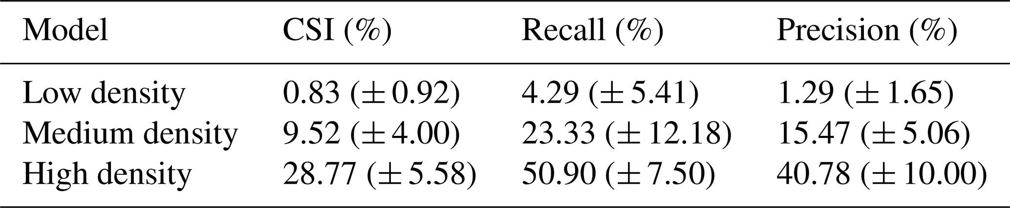
A similar trend is observed in the standard deviation. The low-density model shows very high variance (± 0.92 % CSI), exceeding its own mean value. As the population increases, models become more stable, with standard deviation values that are relatively smaller compared to the mean. However, the absolute SD intervals remain significant even for the best-performing models.

In Fig. 7, we show the performance of the high-density model across the different temporal configurations (test set results), along with a bootstrap variance estimate for each test set. Additionally, we display the overall mean (dotted line) and standard deviation (grey strip) across all configurations. Although no clear trend is observed, we note how the standard deviation intervals of individual configurations (indicated by the error bars) closely align with the overall performance variability across all three metrics. This suggests that once intra-event correlation is accounted for through block bootstrapping, uncertainty within specific time windows matches the overall variability across all temporal configurations. It should be noted, however, that these two types of intervals reflect different sources of uncertainty, with bootstrapping capturing intra-event dynamics, while the overall standard deviation captures performance fluctuations across temporal configurations.

Figure 7 Test set results for all temporal configurations for the high-density model and their variance estimates from bootstrapping. We also highlight the overall mean (dotted line) and standard deviation (coloured strip) across all configurations, and the time period they cover. By allowing temporal overlap, we are able to cover a significant number of days for each configuration, otherwise some splits would contain just a few days or even hours. Also, it is important to note that configurations spanning large periods of time contain many days without rainfall, which are not included in the dataset.

6.1 Baseline comparison

In Fig. 8, our ML approach is compared against the climatology-based baselines. For the high-density group, the ML model outperforms all baselines by a large margin, achieving a CSI 24.35 percentage points higher than FF-EWS, the second-best approach. In the medium-density group, the ML model also obtains substantially better results than the rest, achieving a good balance between recall (23.33 %) and precision (15.47 %). AEMET warnings in this group achieve a much higher recall (+16.11 %) but with very low precision. Finally, for the low-density group, the large variability in all metrics for this group makes it difficult to draw any strong conclusions. While the ML model attains the highest mean CSI, its recall is the lowest among all approaches by a significant margin (14.28 % lower than FF-EWS, which had the second-worst recall). Precision seems to be the determining factor in this case since, despite FF-EWS warnings achieving a slightly higher mean precision (1.32 % versus 1.29 % from the ML model), the ML approach is more consistent (as indicated by the standard deviation intervals), resulting in better results overall.

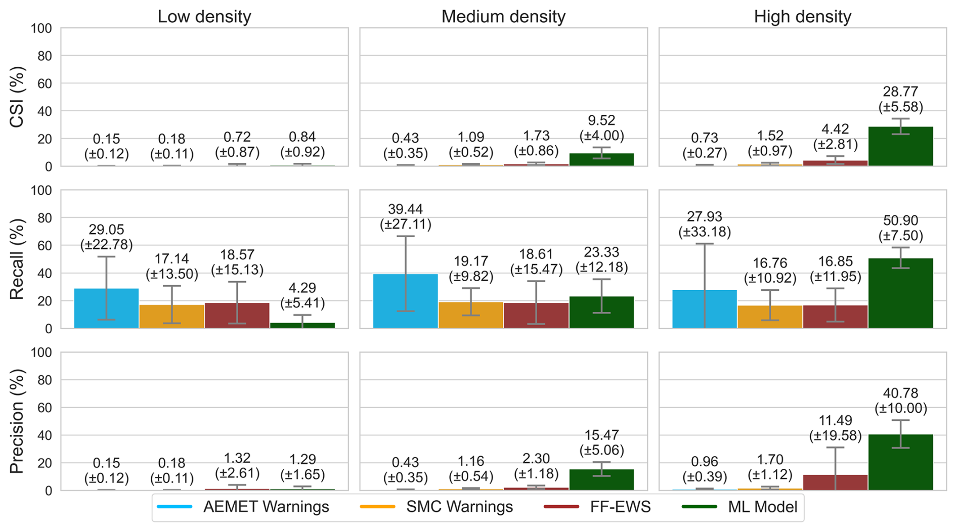
Figure 8 ML model and baseline performance (test set results), across population groups. “AEMET Warnings”, “SMC Warnings”, and “FF-EWS” are the baselines.

6.2 Model explainability

Understanding and interpreting model results is critical for applying ML in a context of Disaster Risk Management. In this section, we will analyse our models' behaviour to discover the performance patterns observed previously.

6.2.1 SHAP feature importance

Figure 9 shows, for each population group model, the ten features with the highest mean absolute SHAP values across all configurations, along with their standard deviation intervals. SHAP (SHapley Additive exPlanations; Lundberg and Lee, 2017) values, a game theory approach, quantify the contribution of each feature to the model's output, assuming a collaborative framework.

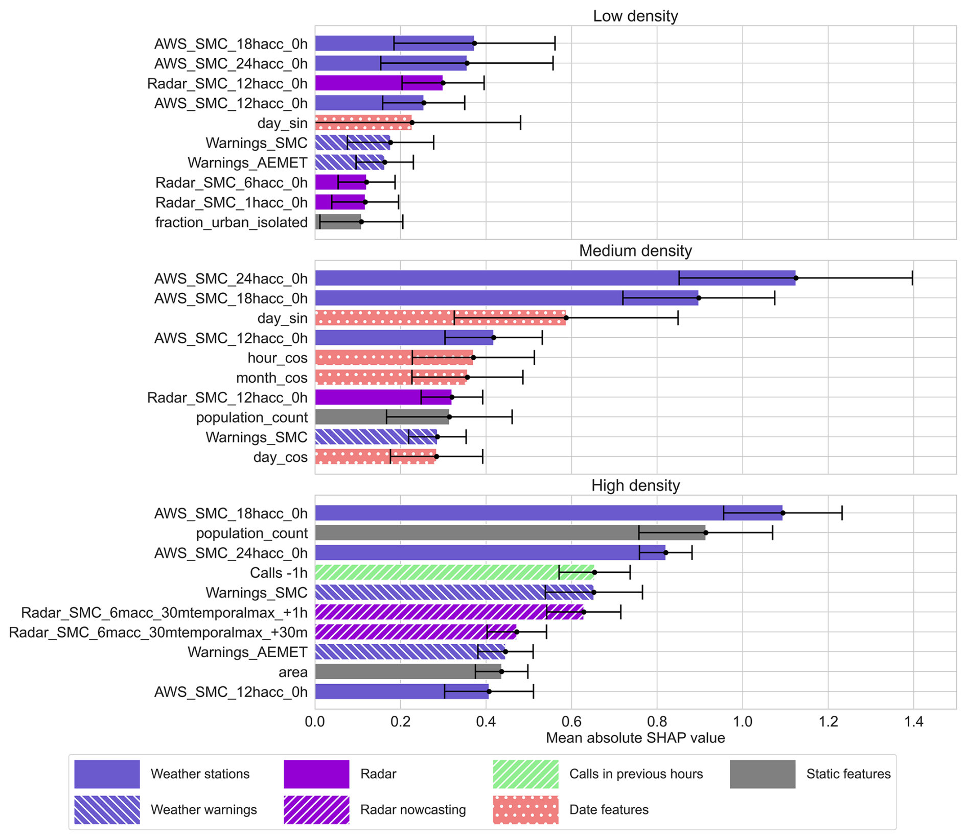
Figure 9 Mean absolute SHAP feature importance value for all three population density models, across all configurations. We also provide the standard deviation intervals. Features are colored based on their general feature group. The higher these values are, the greater its contribution is on the model's output.

This analysis reveals distinct feature importance patterns across population density groups. The low-density model seems to rely mostly on weather features, particularly longer rainfall accumulation periods from automatic weather stations (a trend common also for the rest of models), and official weather warnings. The medium-density model also finds importance in date features (day, hour and month), and in the static population count feature. For the high-density model, we see how, apart from weather station data, the number of inhabitants and the amount of calls received in the previous hour are highly important. Weather warnings remain relevant, and radar nowcasting features, which forecast rain in the target hour, seem to have a significant impact.

However, it is immediately clear that as we move from higher to lower population densities, and consequently from the best- to the worst-performing models, we not only observe smaller absolute SHAP values but also larger variance (as expressed by the standard deviation intervals). This suggests that models with weaker performance struggle to learn consistent relationships between input features and the target, which in turn results in less consistent interpretations.

In Fig. 10, the SHAP values for the models trained on the temporal configurations of the high-density group that obtained the best and worst CSI scores are shown. Both models share similar behaviour, displaying almost the same features in a comparable importance order. Moreover, generally larger values have a stronger contribution towards the positive class, which makes sense considering the features refer to rain accumulation, emergency calls in the previous hours, population, and weather warning level, all indicators of risk. The main difference appears to be in the “Calls -1 h” feature, which indicates the number of emergency calls received in the previous hour. Here, the best-performing model captured a wider range of values, while the worst-performing model was trained on generally smaller values.

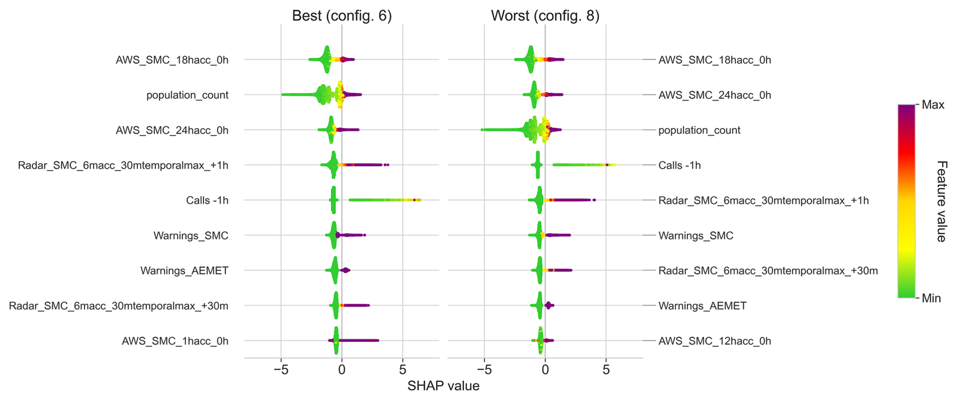
Figure 10 SHAP value comparison between the high-density models trained on the best- and worst-performing temporal configurations. Positive SHAP values indicate a positive impact on the model output (increasing the probability of the positive class), and vice versa for negative values.

6.2.2 Feature group models

To better understand the individual contribution of the different feature types in the data. Models are trained on different feature groups and are then compared with the model trained on all features (Results in Fig. 11). On their own, the number of calls in the past hours has the best prediction capabilities of all feature groups (when considering the mean CSI). This is expected, as the occurrence of emergency calls indicates an ongoing harmful event, increasing the probability that more impacts will follow in the next hours. Even for the medium-density case, a model using only past call data achieves a mean CSI higher than the model trained on all features. This is interesting, as the SHAP analysis for the full medium-density model did not give much importance to this feature group.

Interestingly, weather stations, providing measurements on sparse points in the geography, give better results than radar data, which have more spatial coverage but with a tendency to underestimate rain. This was observed in the SHAP analysis and is again clear for these experiments. Official weather warnings have decent detection capabilities (recall), but the large number of false alarms (low precision) results in a very low CSI when used alone. Other than that, static and time features, as expected, are not useful on their own.

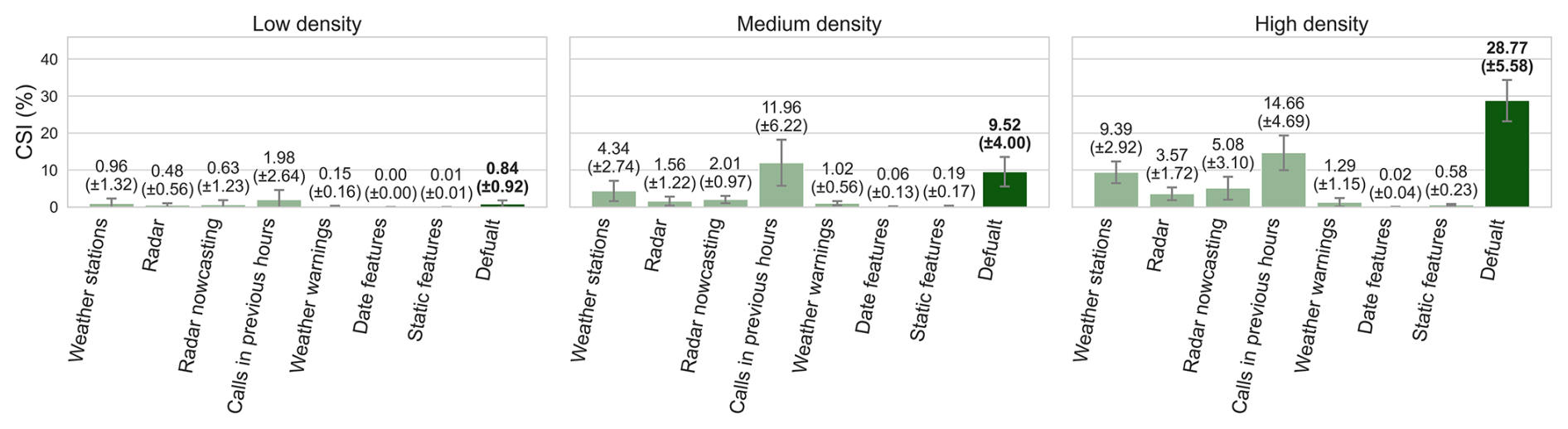
Figure 11 Result comparison of models trained on different feature groups, and the default model, which is trained on all features (in bold)

6.2.3 Ablation study

We now conduct an ablation study to quantify the effect that ignoring particular feature groups has on performance. Results of this can be seen in Fig. 12. If we look at the high-density group, ignoring calls in previous hours has a very negative effect on the model's performance (−11.61 % CSI). Also, weather stations (−6.53 % CSI) seem to be slightly more important than radar (−5.68 % CSI), but overall, the model is capable of using one or the other to provide similar results. The model does not seem to rely much on nowcasting features (−2.74 % CSI). Also notable, static indicators barely contribute to better predictions. We argue that this might be because we already separate municipalities by density, so the model might already have enough population information.

A different picture can be seen in the medium-density case, where ignoring automatic weather station or nowcasting data actually results in slightly better performance overall (+0.79 % and +1.16 % CSI, respectively). This is interesting given that radar data now seem to be the most important group (−3.08 % CSI when ignored), while calls are less relevant in this context (−0.55 % CSI). For the low-density group, the best model results are obtained when static indicators are ignored. However, standard deviations make it hard to confidently draw conclusions for these two population groups.

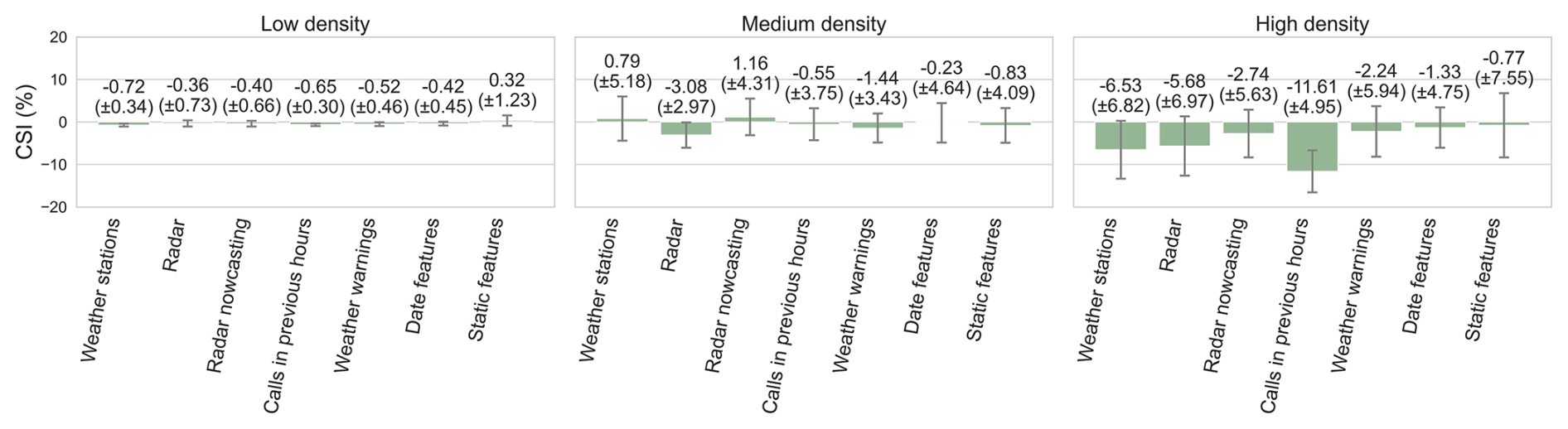
Figure 12 Ablation study, where each bar shows the impact that ignoring that particular feature group has on the overall performance of the ML model trained on all features.

6.2.4 Model performance depending on rain stage

Emergency calls are not always received immediately when rain begins. Their timing can vary considerably, sometimes arriving in the first hour of an event or up to two hours after it ends. To understand model performance through this cycle, we analyse predictions at different stages of a rainfall event, focusing on the high-density model, where patterns are clearest. We define stages per municipality and hour based on observed rain in the last and next hours. We categorise a sample as the “start” if rain began in the target hour after a dry hour, the “end” if rain stopped after a rainy hour, and the hours in between as the “middle”. We also examine the four hours after an event (“after event”), with all other hours classified as “no rain”. We use a rain threshold of 6 mm of rainfall accumulation in one hour, similar to how it was defined in Sect. 4.4.

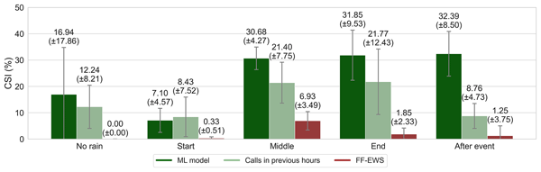
Figure 13 shows a comparison of three approaches on the high-density population group across these stages: our ML model, the model only trained on past calls, and the “FF-EWS” baseline, which obtained the best baseline results. Focusing on the ML approach, the CSI is relatively low at the start (7.10 %) but quickly increases as the event progresses, a pattern that appears more clearly in Fig. 14. This phenomenon mimics a “warm-up” effect. Because the model relies heavily on calls received in recent hours, it experiences a “temporal lag” at the start of an event. It is not until it starts receiving the first impacts (or that the event consolidates and the hazard becomes more apparent), that the model has enough context to make predictions more effectively. However, relying solely on past calls is insufficient, as shown by the inferior performance of the model trained only on call history. While it exhibits a similar pattern, its overall performance is significantly worse (except for a slight improvement at the start), especially after the event, confirming that combining diverse features results in more powerful predictions. For further discussion on the influence of incorporating recent emergency calls as predictors, please refer to Appendix A.

Notably, the ML model maintains a robust performance even after the rain has stopped. In contrast, a climatology-based system such as the “FF-EWS” baseline reaches the best performance during the intermediate stages (6.93 % CSI), but once rain stops, the detection capabilities become severely limited (CSI of 1.85 % and 1.25 % for the “end” and “after event” stages).

It is also interesting that our model struggles more in the first hour (Start) of an event than in hours without rain. This may stem from ambiguity in our definition of when and where it is raining, as some impacts occur with little local rainfall or can be linked to fluvial flooding originating elsewhere. This could also explain the large standard deviation in this stage. Nonetheless, this analysis provides an approximation of the model's behaviour under different stages of a rain event, from which useful insights can be derived.

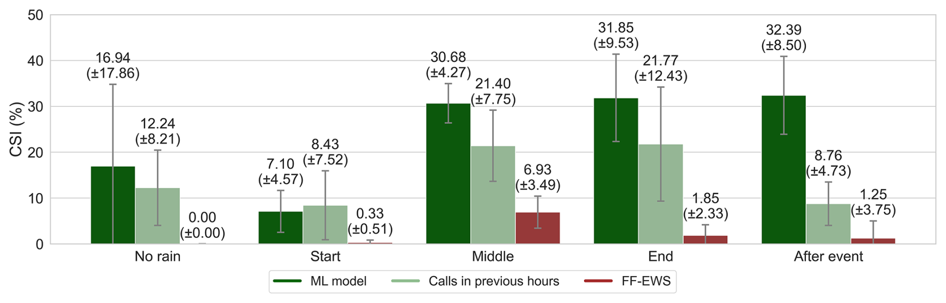
Figure 13 Performance of our ML model, the model trained only on past three hours of call data, and the “FF-EWS” baseline, across the proposed rain stages, on the high-density data partition. The ML approach maintains a high CSI even after rainfall has stopped. A sample is categorised as the “start” if rain began in the target hour following a dry hour, the “end” if rain stopped after a rainy hour, and the hours in between as the “middle”. The four hours following an event are labelled as “after event”, while all other hours as “no rain”.

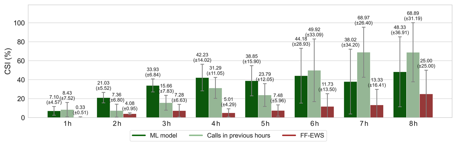
Figure 14 Performance on the high-density population group as the duration of a rainfall event increases, showing the ML model, the model trained only on call data, and the FF-EWS baseline. All approaches go through a “warmup” phase during the first hours, starting with a relatively low CSI, but quickly improving performance as the event lasts longer.

7 Discussion and conclusions

In this work, we have explored how machine learning (ML) models can be used for the hourly prediction of flood-related impacts at the local scale, using high-resolution emergency call data as an impact proxy. To address the varying data availability across the territory, municipalities are divided into three population density groups (Low, Medium, and High), and individual models are trained for each.

We find that ML has great potential for localised impact anticipation where sufficient data exists. Even with a severe class imbalance (a positive rate of around 0.02 %), our high- and medium-density models successfully learn to extract meaningful patterns from the data, improving current methods. However, in extremely low-data scenarios, such as sparsely populated areas like our low-density group, traditional hazard-based methods remain a more reliable tool for identifying general regions of risk. Given the low volume of emergency calls in these areas, training data-driven models with current datasets does not seem realistic.

We compare the proposed ML approaches against traditional, hazard-based methodologies currently in use: official weather warnings issued by the national (AEMET) and regional (SMC) meteorological agencies, and a radar-based river warning product (FF-EWS) used by Catalan civil protection authorities. For high-density areas (containing over 92 % of the total population), the model surpasses all baselines by a large margin across all performance metrics. In medium-density areas, the ML model also substantially outperforms the baselines, notably in achieving a precision of 15.47 %, compared to the 2.30 % of the best-performing baseline. For low-density municipalities, the ML approach obtains the best average Critical Success Index, but this is driven mainly by a higher precision, while its recall is the lowest among all approaches (4.29 %).

Iglesias et al. (2024) explored a similar problem in Catalonia also using 112 emergency calls, proving strong predictive capabilities for severe weather impacts at a daily temporal resolution and municipal scale. The transition to an hourly temporal resolution, despite only targeting flood-related emergencies, allows us to provide more timely and actionable insights into incoming impacts, thereby improving anticipation and readiness. Moreover, our strategy of providing distinct models based on population density allows different behaviours to emerge based on local characteristics. However, shifting to a higher resolution exacerbates the data imbalance problem, as the total number of samples increases significantly while the number of observed impacts remains similar, leading to a higher sparsity. To address this, targeting multiple weather phenomena simultaneously could be beneficial, as it would allow the model to leverage a larger set of impact indicators.

Additionally, we examined the behaviour of the different approaches during different phases of a rainfall event. We observe that all approaches struggle during the first hour of rainfall, showing reduced performance compared to that of the following hours. This is expected, as predicting the onset of impacts is arguably more challenging than predicting their continuation. However, the high-density model still obtains better results than traditional hazard-based methods in this situation, and once the event has started, the performance rises and is maintained even after the rainfall stops, showing promising results for tracking unfolding impacts. Pairing this with explainable AI techniques like SHAP allows for the interpretability of model outputs. In low- and medium-density areas, rainfall-related features appear to have a greater average contribution to the predictions than other variables, largely ignoring static indicators about population. In contrast, the high-density model achieves the most accurate predictions by modulating information on emergency calls in previous hours with weather data and population counts. These findings highlight how interpretability can vary significantly by demographic region. However, since the reliability of SHAP values depends on the model's prediction capabilities, the interpretations from medium- and especially the low-density models must be understood as exploratory insights rather than robust conclusions. This variability underscores the necessity of studying the behaviour of ML systems under different conditions, to correctly support decision-making, instead of simply outputting “solutions”. Ultimately, this analysis intends to build trust in these algorithms by addressing the “black-box” problem (United Nations Advisory Body on Artificial Intelligence, 2024; Scientific Advice Mechanism to the European Commission, 2025; Kox et al., 2025), a requisite for the operational application of any ML-based approach in real-time Disaster Risk Management contexts.

With this paper, we have not only demonstrated the effectiveness of ML for improving impact anticipation, but also highlighted a critical challenge that affects both the adoption of ML-based models, and the broader transition from hazard-based forecasting towards localised impact-based systems: the need for systematic frameworks to collect, share, and integrate diverse impact data sources, such as emergency calls, insurance claims or infrastructure impacts (Kuglitsch et al., 2022; Harrison et al., 2022; Gaztelumendi et al., 2024; Potter et al., 2025; Giner Pérez De Lucia et al., 2026). We argue that combining multiple data sources can overcome the individual limitations of each (for example, the dependence of emergency calls on people reporting) and ultimately build a more complete and homogeneous picture of actual societal impacts. In practice, this translates into two paths for implementation: in data-rich urban areas, models like ours could already be operationalised to improve impact anticipation and warnings, while in more rural regions with data scarcity, the focus should shift towards building the foundational data catalogues this work proves are essential.

7.1 Future work

Future work should explore the effect of varying spatio-temporal resolutions. In particular, adapting the current approach to a higher resolution or making predictions with longer lead times, as this would allow emergency responders more time to prepare for potential emergencies. Utilizing a spatial grid rather than municipalities could benefit the potential applications of this approach, not only allowing for a more in-depth analysis of the optimal spatial resolution, but also potentially making the model more generalizable to other contexts (Kooshki Forooshani et al., 2024), even directly applicable or only require fine-tuning instead of training from scratch.

In addition to refining the model's resolution, the operational evaluation of these systems must be expanded. While the municipality-hour evaluation framework employed in this study provides statistically robust metrics for comparing model performance, it does not fully translate into how emergency managers would perceive the activations (e.g., the number of distinct alerts generated per event). Additionally, evaluating performance across a continuous time period is necessary to better emulate operational deployment, as false alarms could potentially arise from the excluded days with little to no rainfall. Future work focusing on operational deployment should address these limitations in detail, integrating strategies such as event-based evaluation and adequate training protocols to better reflect the real-world management of impactful events.

Moreover, as noted in our discussion, we believe that exploring other impact indicators is critical, as this kind of data is scarce. Different impact data should be studied individually while also assessing how multiple indicators can be combined. On a similar note, this impact modelling should be extended to other natural hazards, either in isolation, as compounding events, or as a cascading succession of hazards (Schroeter et al., 2021).

Finally, in this work, we explored impact modelling through the use of a traditional ML algorithm (XGBoost), working with tabular data. It would be interesting to test the applicability of more complex deep learning models in a context where impact data remains scarce. The use of convolutional neural networks (CNNs) or transformers could allow for more powerful feature extraction, potentially incorporating information from neighbouring areas or past instances to capture complex spatio-temporal patterns. In doing so, explainable AI techniques should continue to be prioritised.

Appendix A: Influence of recent emergency calls

In Sect. 6.2.2, 6.2.3, and 6.2.4 we found that the use of recent calls as a predictor contributes significantly to model performance. In this subsection, we analyze this further by presenting metrics separately for cases where emergency calls were received in the preceding three hours (which serve as input features for the model) and cases where none were received. These results, alongside general model performance, are shown in Fig. A1 as the average across temporal configurations, with error bars indicating the standard deviation.

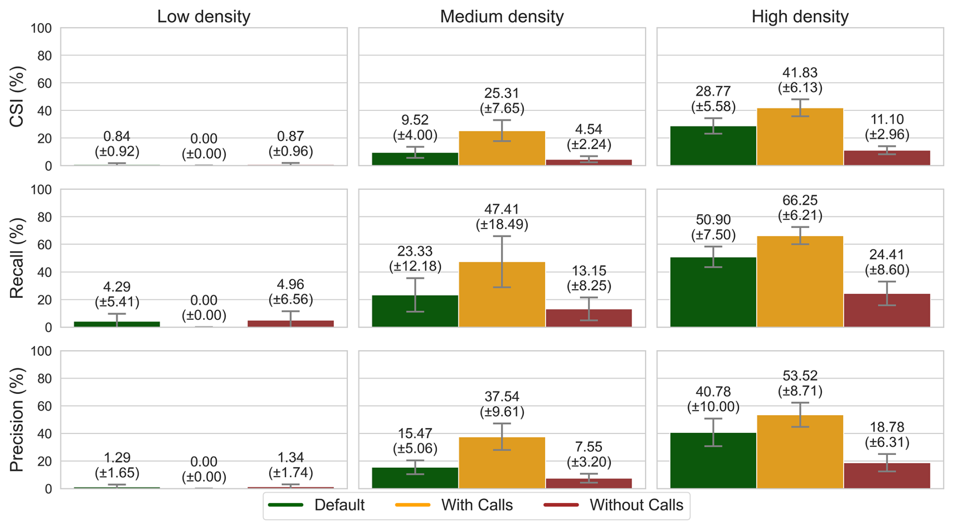
Figure A1 Performance of the ML approaches across population density groups for all data (“Default”), samples with recent emergency calls (“With Calls”), and samples without recent emergency calls (“Without Calls”). Metrics reflect the mean and standard deviation computed across test sets for all temporal configurations.

For the high-density group, results are highest in cases where calls were received, achieving a CSI of 41.84 % compared to 11.10 % without recent calls. This trend is consistent across all three metrics and aligns with the results of Sect. 6.2.4, as at the start of a rainfall event, where generally there are no preceding impacts recorded, performance is worse.

We perform the same study with the model trained without previous call features (from Sect. 6.2.3) and identify a similar pattern of superior performance in situations with continuing impacts (CSI of 27.00 % ± 6.05 % in cases with recent calls versus 8.93 % ± 3.20 % without) for the high-density model. This indicates that while access to recent call history drives significant performance improvements, situations with lingering impacts are inherently easier to predict (coinciding with persistent rainfall that can saturate the soil and drainage systems), even when the model lacks explicit data on these ongoing impacts.

Table A1 Sample counts and positive cases for scenarios with and without recent emergency calls across population density groups (mean ± standard deviation across all temporal configurations).

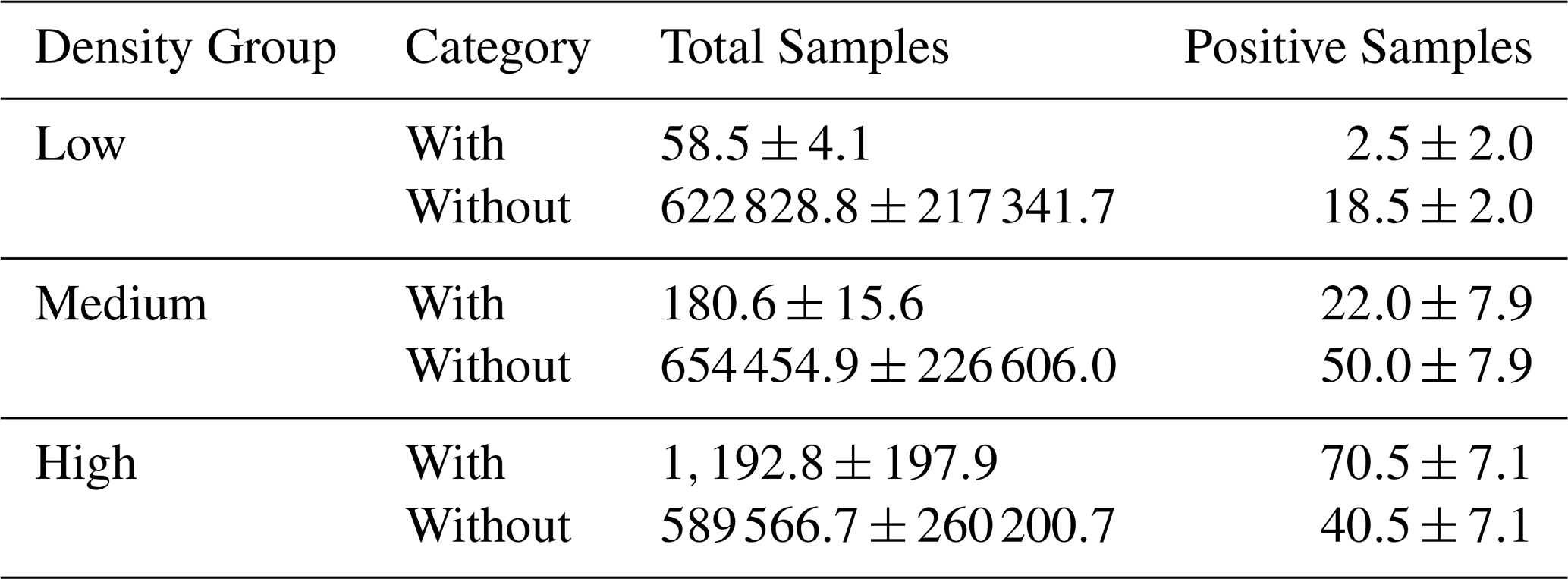
Moving to medium-density populations, we still find that situations with ongoing impacts yield better results. However, the same cannot be said for the low-density group, which achieves a CSI of 0.00 % ± 0.00 %. This discrepancy can be explained by examining the counts of positive cases found in Table A1. In the high-density group, positive samples are more frequent in situations where calls were already received. In contrast, for the medium- and low-density groups, positive samples occur predominantly in cases without recent impacts, indicating that lingering impact events are less common in lower-density regions. Although such events are less frequent in the medium-density group, the model still performs well when they occur. For low-density municipalities, however, these situations are extremely rare, averaging only 2.5 ± 1.96 positive samples with recent impacts across the evaluated time periods.

Appendix B: Model features

A variety of input features were used to effectively identify relationships between weather data, local characteristics, and impact records. Table B1 lists the full set of input features utilised for the machine learning models.

Table B1 Description of model features. Features 1–17 are static, while features 18–54 are dynamic. Features 43–54 represent the pixel-wise temporal maximum over a 30-min window using 6-min rasters, where positive time indices (+) denote forecasts derived from radar nowcasting. “T” refers to the relative prediction time.

Appendix C: Classification and baseline activation thresholds

As explained in Sect. 5, classification thresholds were defined for the ML models, while activation thresholds were defined for every baseline. AEMET utilises a three-level warning system, while the SMC uses a 6-level system. Finally, the FF-EWS takes discrete values representing return periods in years.

Thresholds were chosen by maximizing the Critical Success Index (CSI) on the validation set. The final selections for each approach, population group, and temporal configuration (ten in total) are listed below.

• XGBoost classification thresholds:

  • Low density group: 0.75, 0.825, 0.925, 0.875, 0.875, 0.95, 0.875, 0.925, 0.925, 0.875

  • Medium density group: 0.8, 0.95, 0.875, 0.95, 0.95, 0.95, 0.95, 0.925, 0.95, 0.95

  • High density group: 0.725, 0.95, 0.825, 0.95, 0.95, 0.95, 0.95, 0.95, 0.95, 0.90

• AEMET warning level activation thresholds:

  • Low density group: 3, 3, 3, 2, 2, 2, 2, 2, 2, 2

  • Medium density group: 2, 3, 3, 3, 2, 2, 2, 2, 2, 2

  • High density group: 2, 2, 3, 3, 3, 3, 3, 3, 2, 2

• SMC warning level activation thresholds:

  • Low density group: 5, 5, 5, 3, 3, 4, 4, 4, 4, 4

  • Medium density group: 5, 5, 5, 5, 4, 4, 6, 6, 6, 4

  • High density group: 5, 5, 5, 4, 4, 6, 6, 6, 3, 3

• FF-EWS return period activation thresholds (in years):

  • Low density group: 2, 10, 10, 10, 5, 2, 2, 2, 10, 10

  • Medium density group: 2, 2, 2, 10, 10, 10, 10, 5, 5, 5

  • High density group: 2, 10, 10, 10, 10, 10, 10, 2, 2, 10

Appendix D: Temporal configuration details

Figures D1, D2, and D3 show the temporal configurations used for the low-, medium-, and high-density population groups. Our evaluation scheme ensures that all validation and test sets contain the same number of positive samples, while also helping to cover comparable time periods encompassing multiple months. This latter part, however, is not always possible, as large concentrations of impacts can occur within a small time window, as observed, for example, in the final configurations of Fig. D3. This period coincides with the last months of 2024 and the severe DANA event that affected the Spanish Mediterranean coast (Spanish National Meteorological Agency (AEMET), 2024).

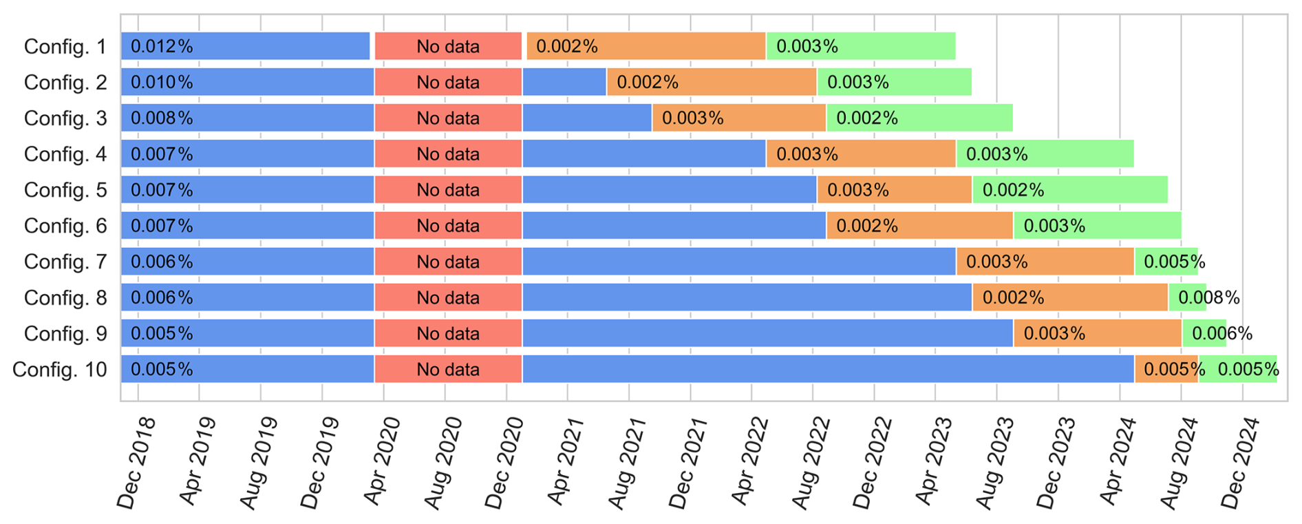
Figure D1 Temporal configurations used for the low-density data group. The timelines for training (blue), validation (orange), and testing (green) are indicated, along with the percentage of positive samples in each. The data gap is highlighted in red. All validation and test sets contain 21 positive samples. Note that not all days are included in the dataset, only those with sufficient daily rain accumulation are retained (see Sect. 4.4).

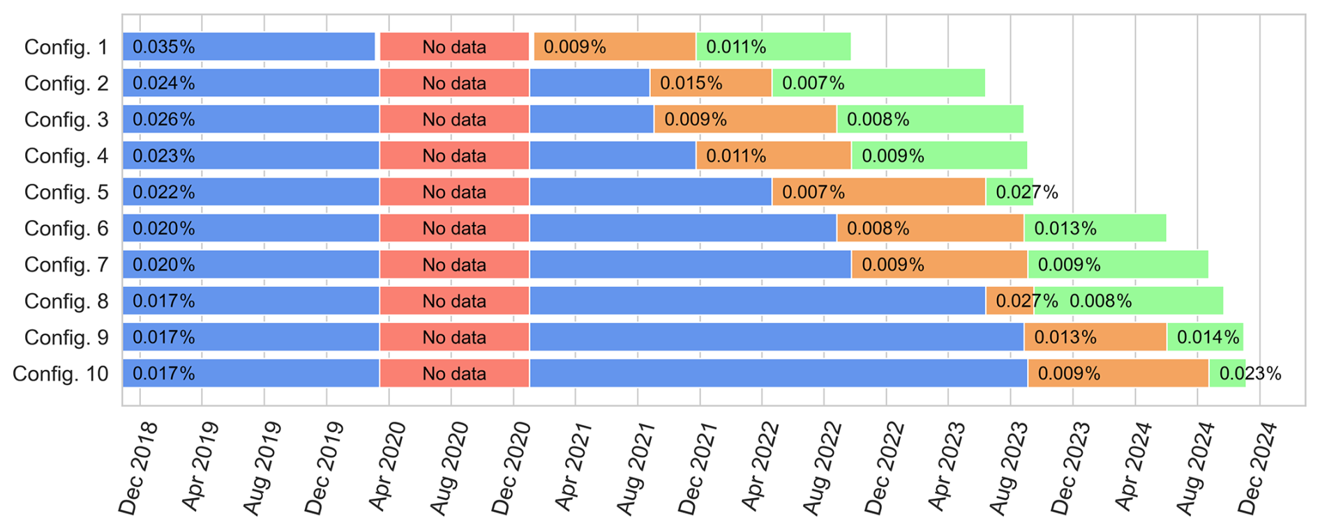
Figure D2 Temporal configurations used for the medium-density data group. The timelines for training (blue), validation (orange), and testing (green) are indicated, along with the percentage of positive samples in each. The data gap is highlighted in red. All validation and test sets contain 72 positive samples. Note that not all days are included in the dataset, only those with sufficient daily rain accumulation are retained (see Sect. 4.4).

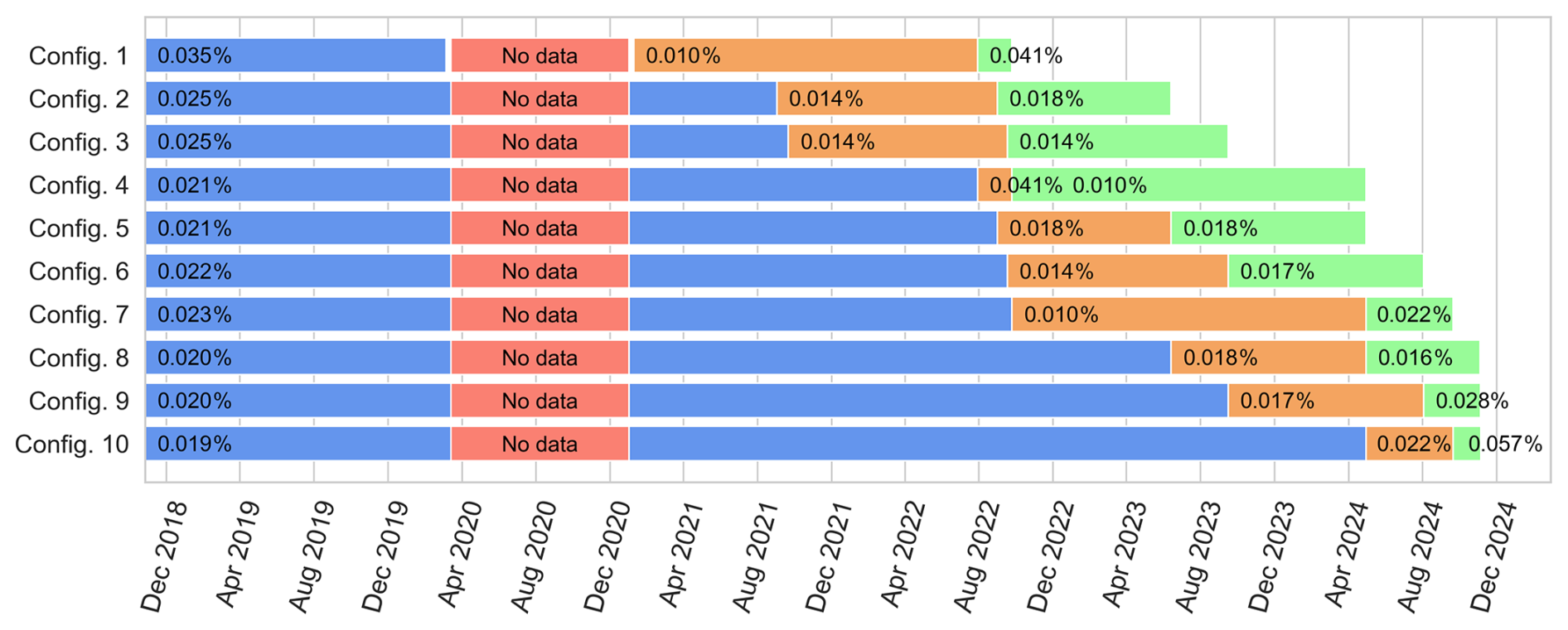
Figure D3 Temporal configurations used for the high-density data group. The timelines for training (blue), validation (orange), and testing (green) are indicated, along with the percentage of positive samples in each. The data gap is highlighted in red. All validation and test sets contain 111 positive samples. Note that not all days are included in the dataset, only those with sufficient daily rain accumulation are retained (see Sect. 4.4).