Potential glacier contributions to the 2024 La Bérarde flood

On 20–21 June 2024, an unprecedented flood of the Etançons river caused important damage to the village of La Bérarde (Écrins, France). An analysis of the event showed that the flood was caused by the combination of an intense rain-on-snow event at high altitude and the subglacial drainage of a supraglacial lake from Glacier de Bonne Pierre. In this study, we quantify the water volume that could have also been trapped beneath the glacier in local minima of the hydraulic head, i.e., in locations that could host so-called glacier water pockets impounded by hydraulic barriers. In the absence of direct observations of water pockets, we use a numerical, steady-state approach that computes the subglacial hydraulic head from surface and bedrock topography of Glacier de Bonne Pierre. As of June 2024, hydraulic barriers at Glacier de Bonne Pierre could, in theory, have impounded water volumes on the order of 10⁵ m³, with the largest modeled water pocket beneath a surface depression that temporarily hosted a supraglacial lake. These results provide a first-order estimate of the potential subglacial water storage capacity prior to the June 2024 flood. We propagate uncertainties in surface elevation, bedrock elevation, and flotation fraction (the ratio of basal water pressure to ice overburden pressure) through a stochastic framework and show that spatial variability in the flotation fraction dominates the uncertainty in the resultant water-pocket volume. This highlights the strong sensitivity of subglacial water-routing results to poorly constrained basal water pressure conditions. While acknowledging that the actual presence and contribution of such water pockets cannot be confirmed from available observations, our study highlights the glacial flood potential of debris-covered glaciers with pronounced surface topographic depressions, which can promote both supraglacial and subglacial water storage.

1 Introduction

On the night of 20–21 June 2024, an unprecedented flood impacted the village of La Bérarde (1727 m a.s.l., Écrins, France, see Fig. 1). The flood and associated sediment deposition buried large parts of the village. No fatalities occurred due to early evacuation of residents. A retro-analysis of the event (Blanc et al., 2024; Filhol et al., 2026) attributed part of the flood to the concurrence of rare hydro-meteorological conditions: an anomalously thick late-spring snowpack, an intense snowmelt event due to high temperatures, and a large cumulative amount of rain during the 48 h preceding the event. Hydrological modelling accounting for rainfall and snowmelt alone do not match the timing of the discharge increase observed in the Veneon River at Les Étages and the timing of the first flooding and sediment deposits at La Bérarde (see details in Sect. 2). This mismatch, together with geomorphological evidence observed in the Torrent de Bonne Pierre, suggests the contribution of an additional water reservoir from Glacier de Bonne Pierre, located 2 km upstream of La Bérarde. Observations of the glacier surface before and after the flood indicated the subglacial drainage of a temporary supraglacial lake with a volume of ≈ 100 × 10³ m³, which likely constituted a major component of the additional water released during the event. However, the available data and observations did not allow to determine whether the glacier has released more water than the lake alone. Moreover, this supraglacial lake forms every summer and has been observed to drain subglacially in previous years without causing glacial outburst floods.

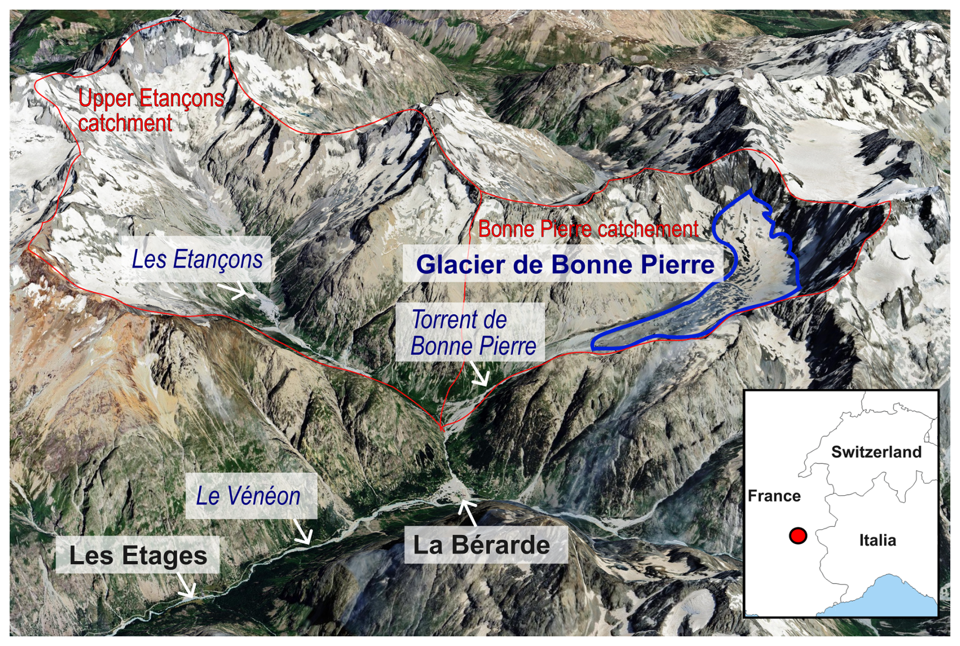
Figure 1 3D view of the upper Vénéon valley and contributing catchments of the 20–21 June 2024 flood. Glacier de Bonne Pierre outline is shown in blue (hand-drawn). The catchment boundaries of upper Étançons and Bonne Pierre are shown in red. River names are written in italic. Image acquired on 17 July 2024 (imagery © 2024 Airbus, map data © 2024 Google).

In this context, we investigate the possibility of a water pocket outburst flood (WPOF) originating from Glacier de Bonne Pierre on 21 June 2024. WPOFs are glacial outburst floods that originate from the rupture of a water pocket within the glacier (Ogier et al., 2025). Water pockets are water-filled englacial or subglacial reservoirs and are, by definition, not visible from the glacier surface. WPOFs can be sudden and dangerous (e.g., Tête Rousse in 1892; Vincent et al., 2010). WPOFs differ from glacier lake outburst floods (GLOFs; Roberts, 2005; Björnsson, 2010; Carrivick and Tweed, 2016; Emmer et al., 2022; Zhang et al., 2024), for which the floodwater originates from a visible reservoir on the glacier surface or margins, or from a subglacial lake formed by geothermal heat (Björnsson, 2010). Although WPOFs have been documented (Haeberli, 1983; Vincent et al., 2010, 2012; Deline et al., 2004; Ogier et al., 2025), the mechanisms of formation and rupture of water pockets are still poorly understood due to a lack of direct observations. Four distinct mechanisms for the formation of a water pocket have been suggested based on a literature review and an inventory of 91 reported WPOFs in the Swiss Alps (Ogier et al., 2025). These four mechanisms represent the filling of an en- or subglacial water reservoir caused by: (1) temporary blockage of subglacial channels, where ice collapses from the roof of a subglacial channel or a large cavity and creates a temporary ice dam that traps water and causes a sudden outburst when the dam fails; (2) hydraulic barriers, where water accumulates at a local minimum of the subglacial hydraulic head, the surrounding ice acts as a dam until the water pressure exceeds the ice overburden pressure and triggers an outburst; (3) water-filled crevasses, where isolated crevasses fill with water and reconnect to the drainage system via hydrofracturing to cause an outburst; and (4) thermal barrier, where water is trapped at the temperate-to-cold interface in a polythermal glacier (as for Glacier de Tête Rousse; Vincent et al., 2010; Gilbert et al., 2012; Vincent et al., 2015), leading to an outburst due to the mechanical failure of the ice dam or when the ice warms to the pressure-melting point.

Glacier de Bonne Pierre is assumed to be temperate – given its elevation and evidence of water at the glacier base – which makes the presence of a thermal barrier unlikely. Water pockets caused by temporary blockage of subglacial channels are short-lived water bodies and cannot be directly assessed in the absence of in situ observations during the event; therefore, we cannot evaluate this formation mechanism within the scope of this study. Water-filled crevasses are unlikely in Glacier de Bonne Pierre due to the general absence of significant crevasses at the surface. In contrast, the potential volume of water pocket impounded in a hydraulic barrier can be estimated using surface and bedrock topography. Moreover, the low surface slopes, debris cover, and pronounced surface depressions of Glacier de Bonne Pierre are favourable for the presence of hydraulic barriers.

The aim of this study is to estimate the maximum potential water volume impounded by hydraulic barriers in Glacier de Bonne Pierre. Our approach is purely geometrical and steady-state: it relies on surface and bedrock topography, which makes it easily transferable to other glacier settings. The resulting volumes therefore represent a first-order estimate of the potential water storage capacity of hydraulic barriers prior to the June 2024 flood event, rather than a reconstruction of the actual filling or rupture processes associated with the flood. This approach allows us to assess whether, in theory, water pockets of significant volume could have existed prior to the flood event. We explicitly propagate input uncertainties using a stochastic approach, providing an assessment of their influence on the volume of the resulting water pockets. We then discuss the possible contribution of such water pockets to the observed flood at La Bérarde.

2 The June 2024 La Bérarde flood

La Bérarde is a hamlet of Saint-Christophe-en-Oisans located in the upper Vénéon valley (Écrins massif, French Alps), and Glacier de Bonne Pierre is a 1.74 km² mountain glacier located 2 km upstream of it (Fig. 1). The glacier drains into the Torrent de Bonne Pierre, a tributary of the Étançons River, which flows into the Vénéon River. The glacier tongue is characterized by low surface slopes, debris cover, and pronounced surface depressions.

On 20–21 June 2024, a major debris flow caused the partial destruction of the village of La Bérarde. The event is described in detail in a companion study that quantifies the hydrological and geomorphological drivers of the flood and the role of sediment connectivity between the source area and the village (Filhol et al., 2026). In summary, the meteorological and snow conditions during the flood events were characterized by an anomalously large (estimated return period of 15–20 years) late-spring snowpack at high elevations, an intense snowmelt driven by warm air masses from 18 June onwards (with melt rates between 19 and 21 June corresponding to a return period of 20 years), and cumulative precipitation of approximately 130 mm over 48 h in the Étançons catchment (with a return period estimated at around 10 years for the station at Saint-Christophe-en-Oisans – 10 km downstream to La Bérarde), with a rain-snow line around 3500/4000 m a.s.l. The concurrence of strong snowmelt and heavy precipitation resulted in a high water input to the catchment.

Peak discharge estimates during the flood are associated with large uncertainties due to intense sediment transport and changes in channel cross section during the event. In the upper Étançons catchment, upstream of the confluence with the Torrent de Bonne Pierre, the peak discharge of the Étançons river was estimated to be between 15 and 40 m³ s⁻¹ based on flood marks. Downstream of the confluence with Torrent de Bonne Pierre, discharge estimates are highly uncertain. Nevertheless, geomorphological evidence indicates that the Torrent de Bonne Pierre was the dominant source of sediment during the event. The total sediment volume exported by the Torrent de Bonne Pierre is estimated to be ≈ 300 × 10³ m³ over a reach of approximately 1.2 km, with local incision reaching up to about 10 m (Mainieri et al., 2025).

The hydrological model MORDOR-SD (Garavaglia et al., 2017), a semi-distributed elevation-band model that represents the main hydrological processes in mountain catchments (including snow accumulation and melt, runoff, groundwater storage, and glacier melt), was used to simulate the hydrological response of the catchment and to attribute the relative contributions to the flood. However, the simulated flood volume cannot be directly compared with the observed flood volume, as the water budget cannot be closed because of large uncertainties in discharge estimates, which are caused by both the limitations described above and the failure of the gauging station at Les Étages during the flood. Nevertheless, the model provides useful information on the timing of the discharge response, indicating that the abrupt rise observed at Les Étages during the night of 20–21 June (before the station failed) cannot be explained by precipitation and snowmelt alone. This suggests a contribution from a glacial reservoir located at Glacier de Bonne Pierre, consistent with the large debris-flow contribution from the Torrent de Bonne Pierre (visible in Fig. 1).

A supraglacial lake located on the tongue of Glacier de Bonne Pierre was observed on 18 June, with an approximate volume of 100 × 10³ m³. The lake had emptied by 22 June, implying drainage sometime during this interval. Since 2016, this lake has been observed to slowly drain subglacially and annually, but without any reported downstream impacts. Based on this usual slow drainage mode, it is possible that the dynamic of the lake drainage in 2024 was different in comparison to previous years. Moreover, we suggest that water stored subglacially may have additionally contributed to the glacial flood.

3 Methods

3.1 Overview

To assess the additional, potential water contribution that may have been stored subglacially, we estimate the maximum volume of subglacial water pockets that could have been impounded by hydraulic barriers. First, we measured ice thickness at discrete locations using airborne ground penetrating radar (GPR). Second, we interpolated ice thickness over the glacier using a mass-conservation approach, and thereby obtained a distributed bedrock topography by subtracting ice thickness from the glacier surface elevation. Third, we calculated the subglacial hydraulic head as a function of surface and bedrock topography using the Shreve (1972) approximation, which assumes that basal water pressure equals the ice overburden pressure. Fourth, we computed the maximum water volume by geometrically filling each closed depression in the hydraulic head field with an equivalent water column up to its spill point. We did this by assuming hydrostatic equilibrium between water pressure and ice overburden pressure, and the resulting subglacial water reservoirs are referred to as water pockets. Fifth, we estimated uncertainties in the total subglacial water storage estimate using a Monte Carlo approach to propagate uncertainties from surface elevation, bedrock elevation, and basal water pressure to the hydraulic head field. These five steps are detailed in the following subsections.

Our numerical approach intentionally represents a steady-state configuration of the subglacial drainage network and does not aim to reproduce the highly dynamic, time-dependant physical processes occurring during the flood event (e.g., enlargement of subglacial channels, ice creep, and transient reorganization of the drainage network). While physically-based models capable of representing some of these processes exist (see Flowers, 2015, for a review), their outcomes would be highly sensitive to stochastic, small-scale processes related to water routing that are neither directly observable nor straightforward to parameterize. The application of such models to real alpine glacier settings remains strongly limited by data availability (such as exact bedrock topography) and the difficulty of constraining initial and boundary conditions at the required spatial and temporal scales. Therefore, our approach focuses on estimating the maximum potential storage capacity of hydraulic barriers given the geometric inputs available for Glacier de Bonne Pierre.

3.2 Glacier surface topography and ice thickness measurements

Glacier surface topography is known for the dates of 28 June 2024 (1 week after the outburst) and of 28 October 2024 (Fig. 2a), when digital elevation models (DEMs) were reconstructed from airborne light detection and ranging (LiDAR) data. These DEMs have a horizontal resolution of 1 m and a maximum per-pixel elevation error of 0.2 m (June) and 0.1 m (October), with an average error of a few millimeters in both cases. The DEM acquired on June 2024 is incomplete, as it does not cover the uppermost, steeper part of the glacier. The DEMs acquired in June and October are used for the calculation of subglacial hydraulic potential and distributed bedrock elevation, respectively.

Although the June DEM was acquired one week after the flood event, we expect negligible changes in glacier surface elevation during this short interval because surface melt was small. Localized surface changes may have occurred in the vicinity of the supraglacial lake, for example due to crevasse formation associated with the lake's subglacial-drainage, although there was no clear evidence of such crevasses after the event. (Filhol et al., 2026) shows that between 2024 and 2021, the largest surface elevation differences occurred at the exact location of the supraglacial lake, with a cumulative lowering of approximately 15 m. This ablation hotspot is likely explained by progressive melt related to the development of ice cliffs (i.e., increased melt where cliffs steepen and become debris-free). While a similar process might have occurred in June, we assume it to be negligible over the course of a week.

Ice thickness was measured along 28 profiles using ETH's helicopter-borne GPR system “AIRETH” (e.g., Langhammer et al., 2019b; Grab et al., 2021; Farinotti et al., 2025; Santin et al., 2026). The GPR survey was conducted on 6 November 2024. The GPR system (PulseEkko, Sensors & Software) was operated with two orthogonal bistatic dipole antenna pairs at a central frequency of 50 MHz. This frequency corresponds to an electromagnetic wavelength of ≈ 3.4 m in ice and represents a compromise between the targeted ice-depth reflections and spatial resolution. In addition to ice thickness measurements, the survey was also designed to identify potential GPR signal indicative of englacial or subglacial water. The data acquired by the AIRETH system were processed in two main steps: (i) reconstruction of the positioning and (ii) GPR signal processing. First, the 3D coordinates and orientation of the GPR antennas were reconstructed at 1 Hz resolution by combining the 4 onboard Global Navigating Satellite System (GNSS) sensors, an IMU (inertial measurement unit), a laser altimeter, and a local differential GNSS base station. These data were used to project each trace onto the glacier surface and synchronize it with the GPR timestamps. Second, the GPR signal was processed following a standard radar processing workflow to improve signal–to–noise ratio and enable clear interpretation. For this, we employed our in-house Matlab-based toolbox GPRglaz and follow the processing workflow typically used for similar field-based investigations (e.g., Church et al., 2020; Grab et al., 2021; Ogier et al., 2023). The processing steps include: (1) time zero correction based on the arrival of the direct wave, (2) removal of background noise using an optimized procedure based on singular value decomposition filtering, (3) Butterworth bandpass filtering (10–200 MHz) to cut undesirable low and high frequencies, (4) trace binning at a spatial sampling rate of 0.5 m for regular sampling, (5) surface reflection picking based on laser altimetry, and (6) time–to–depth conversion using Kirchhoff migration (Margrave and Lamoureux, 2019), assuming constant radar wave velocity (0.167 m ns⁻¹ for ice; Glen and Paren, 1975).

3.3 Interpolated ice thickness and bedrock elevation using GlaTE

The ice thickness retrieved through the workflow described in the previous section is then used to constrain a glacier-wide ice thickness distribution. For this we used the Glacier Thickness Estimate (GlaTE, Langhammer et al., 2019a) algorithm, following the same approach as Grab et al. (2021). In summary, GlaTE performs a physically based interpolation of ice thickness by combining GPR observations with glaciological modeling constraints derived from surface topography, apparent mass balance, and Glen's flow law, which are used to estimate basal shear stress and ice fluxes. The digitized glacier outline of Glacier de Bonne Pierre was taken from the Global Land Ice Measurements from Space portal (Raup et al., 2007) and refers to the year 2022. The resulting distributed ice thicknesses were generated at a spatial resolution of 10 m on a regular grid, consistent with the smoothing applied in the GlaTE algorithm and the typical spacing of the GPR profiles. The distributed ice thickness is subtracted from the glacier surface elevation acquired in October 2024 to obtain a distributed bedrock topography.

3.4 Deterministic hydraulic head and subglacial water routing

We write the subglacial hydraulic head ψ (i.e. the hydraulic potential expressed in meters water-equivalent) as

$$\begin{array}{}\text{(1)}& \mathit{\psi }={\displaystyle \frac{p_{\mathrm{w}}}{{\mathit{\rho }}_{\mathrm{w}}g}}+z_{\mathrm{b}},\end{array}$$

where p_w is the water pressure, ρ_w the density of water, g the gravitational acceleration, and z_b the bedrock elevation (Cuffey and Paterson, 2010). We assume that water pressure is a function of ice overburden pressure (p_i), such that p_w = f p_i, with f the flotation fraction, i.e., the ratio of basal water pressure to ice overburden pressure. The hydraulic head then becomes:

$$\begin{array}{}\text{(2)}& \mathit{\psi }=f{\displaystyle \frac{{\mathit{\rho }}_{\mathrm{i}}}{{\mathit{\rho }}_{\mathrm{w}}}}\left(z_{\mathrm{s}}-z_{\mathrm{b}}\right)+z_{\mathrm{b}},\end{array}$$

where ρ_i is the ice density (910 kg m⁻¹), and z_s the glacier surface elevation. The commonly-used Shreve approximation is obtained for f = 1 (Shreve, 1972).

Here, we use the package WhereTheWaterFlows.jl (WWF) and its subglacial routing module WhereTheWaterFlows.Subglacially (WWFS) to compute subglacial water routing (see Data and Code availability). WWFS implements Eq. (2) using a D8 flow-routing algorithm (O'Callaghan and Mark, 1984) and calculates the upslope area catchment for each pixel. Larger upslope areas are interpreted as indicating larger volumes of subglacial water routed through a given pixel. These flow patterns are assumed to represent the steady-state configuration of the distributed subglacial drainage system; they do not account for the geometry of subglacial channels. Examples of applications of this approach in glacier hydrology can be found in Sharp et al. (1993); Flowers and Clarke (1999); Fischer et al. (2005); Chu et al. (2016); Mankoff et al. (2020); Malczyk et al. (2023); Horgan et al. (2025); Ogier et al. (2025).

The inputs of WWFS are the surface and bedrock elevations presented in the previous sections, with the following additions: the bedrock elevation was resampled to a 1 m grid using bilinear interpolation to match the spatial resolution of the surface elevation. We applied a moving-average boxcar filter to the surface elevation that is equal to 10 % of the local ice thickness at each grid cell. This is because the high-resolution surface elevations are sensitive to unwanted local features in the water routing calculation, such as crevasses, boulders or moulins. This filter also has a physical meaning because, in reality, the basal water pressure is modulated by the ice thickness through mechanical stress redistribution, such that small and local features at the ice surface do not impact the basal conditions. The sensitivity to this arbitrary choice for the resulting water-pocket volume impounded by hydraulic barriers is discussed in Sect. 5.2.

3.5 Water-pocket volume estimation

Subglacial water pockets impounded by hydraulic barriers form in areas corresponding to local minima in the hydraulic head, as defined by Eq. (2). The subglacial water-pocket height, i.e., the vertical distance between the bedrock and the water-filled cavity ice-roof, is obtained by filling closed depressions in the hydraulic head field (as in Ogier et al., 2025). For each closed depression, water accumulates until it reaches a limiting hydraulic head value, defined by the hydraulic head at the seal, i.e., the ice dam. This limiting value represents the maximum hydraulic head that can be retained by the hydraulic barrier and is denoted as ψ_filled. The subglacial water-pocket height h_wp at each pixel (x,y) is then given by the difference between ψ_filled and the local hydraulic head ψ(x,y):

$$\begin{array}{}\text{(3)}& h_{\mathrm{wp}}(x,y)={\mathit{\psi }}_{\mathrm{filled}}(x,y)-\mathit{\psi }(x,y).\end{array}$$

The total water volume V_wp is then obtained by summing the water-pocket height over the water-pocket domain Ω (i.e., the area where h_wp > 0):

$$\begin{array}{}\text{(4)}& V_{\mathrm{wp}}=\sum _{(x,y)\in \mathrm{\Omega }}{h}_{\mathrm{wp}}(x,y)\mathrm{\Delta }A,\end{array}$$

where ΔA is the area of one grid cell (1 m² in this study). This volume computation implicitly assumes a slow filling process such that the ice roof can uplift and remain in hydrostatic equilibrium with the underlying water.

3.6 Stochastic hydraulic head and subglacial water routing within uncertainties

Finally, we quantify how uncertainties in the input variables affect the predicted hydraulic potential and the resulting volume of subglacial water pockets. These variables are the glacier surface elevation (z_s), the bedrock elevation (z_b), and the flotation fraction (f). We perform forward error propagation using the Monte Carlo module WhereTheWaterFlows.Randomly implemented in WWF. For each realization, we generate a perturbed field z^* as follows:

$$\begin{array}{}\text{(5)}& \begin{array}{rl}& z^{*}(x,y)\\ & =\left\{\begin{array}{ll}z(x,y)+\mathit{\sigma }(x,y)\mathit{ϵ}(x,y),& \text{for}z\in \mathit{\{}{z}_{\mathrm{b}},f\mathit{\}},\\ z_{\mathrm{s},k}(x,y),k\in \mathit{\{}\mathrm{0},\mathrm{10},\mathrm{20},\mathrm{\dots },\mathrm{100}\mathit{\}},& \text{for}z=z_{\mathrm{s}}.\end{array}\right.\end{array}\end{array}$$

where z is the original field value at coordinates (x,y) (e.g., z_b, z_s or f), and ϵ(x,y) is a zero-mean, unit-variance Gaussian random field. For z_b and f, independent Gaussian random fields are generated using their respective uncertainty amplitude fields σ(x,y), which represent the local standard deviation of the error, together with a spatial correlation length that defines the scale over which errors are correlated. The estimation of these quantities is key to providing uncertainty estimates and is detailed in Appendix A. Unlike z_b and f, the uncertainty in z_s is not represented through random perturbations, as it arises from the choice of a moving-average boxcar filter applied to the surface DEM. This filter is intended to remove small-scale roughness not expected to influence the subglacial hydraulic head, and its window size, k, is expressed as a fraction of the local ice thickness (set to 10 % in the deterministic case). We account for surface uncertainties by generating an ensemble of surface DEMs, z_s,k, with k ranging from 0 % to 100 % in increments of 10 %. For each realization, the value of k is sampled uniformly from this discrete set.

The only input parameters not constrained by observations at Glacier de Bonne Pierre are the prescribed spatial variations in the flotation fraction within the associated range [0.9–1.1], with a correlation length of 100 m. This arbitrary choice reflects the lack of direct measurements of basal water pressure and is discussed in Sect. 5.2.

4 Results

4.1 GPR observations, ice thickness and bedrock elevation

Distributed ice thickness and bedrock elevation results from GlaTE are shown in Fig. 2b and c, respectively. The total length of GPR profiles having interpretable ice thickness measurements is 10  km (black lines in Fig. 2c), corresponding to 51 % of the total survey distance (grey lines in Fig. 2c). As of October 2024, i.e. the date of the surface DEM used in GlaTE to subtract the ice thickness, the maximum ice thickness was 134 m and the mean ice thickness was 54 m. Point-scale uncertainties in bedrock elevation reach up to 24 m and are found at locations that are most distant from GPR measurements (Fig. 2d). Bedrock elevation uncertainties are detailed in Appendix A.

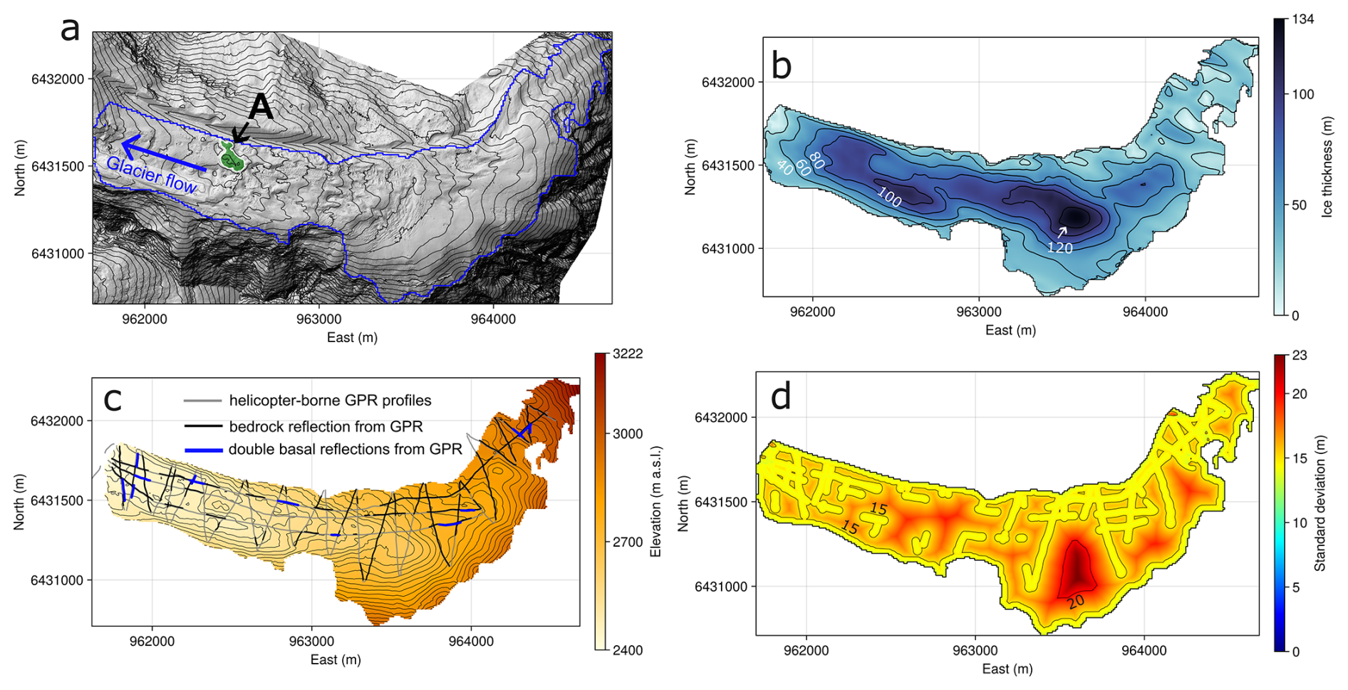
Figure 2 Surface elevation hillshade (a), ice thickness (b), bedrock elevation (c), and bedrock elevation uncertainties (± standard deviation) (d) for Glacier de Bonne Pierre in October 2024. Black and blue lines in panel (c) indicate where bedrock elevation was obtained by GPR measurements; blue lines indicate where double basal reflections from GPR suggest the presence of subglacial channels. The letter A in panel (a) marks the location of the supraglacial lake that drained during the flood event in June 2024 (lake area in green). Contour intervals are 20 m for panels (a), (b) and (c), and 10 m for panel (d). The glacier outline refers to the year 2022.

Figure 2c shows the locations where the radargrams display double basal reflections, i.e., two basal reflectors on top of each other that are vertically separated by typically a few meters (after time–depth conversion using a constant electromagnetic wave velocity in ice). We interpret these reflectors as the ice–water and water–bedrock interfaces of subglacial channels (e.g., Church et al., 2021). No water-filled reservoirs or empty subglacial cavities were detected along the surveyed profiles. Note, however, that the absence of strong reflections in the radargrams does not necessarily imply the absence of subglacial water, water pockets or empty cavities, as the signal could be substantially attenuated by water inclusions (Ogier et al., 2023) and/or debris (Santin et al., 2024). This likely explains the large absence of specular reflections in the GPR profiles (grey lines in Fig. 1c). A denser network of GPR profiles would likely be required to resolve three-dimensional features such as a water pocket (Vincent et al., 2012) or an empty subglacial cavity (Ruols et al., 2025).

Overall, there is good agreement between indications of subglacial water from GPR and the subglacial water paths predicted from the hydraulic head field (see next section, Fig. 3). A notable deviation appears at the glacier tongue, where subglacial water indications from GPR are wider than the modeled subglacial water paths. This is because the modeled paths represent preferential flow directions derived from the hydraulic head field using a steepest-gradient (D8) algorithm, rather than actual subglacial channel geometry. The existence of wide subglacial channels near the glacier terminus or under shallow ice is consistent with observations in alpine glaciers, where subglacial drainage often develops into wide, shallow conduits rather than narrow channels (e.g., Church et al., 2020; Egli et al., 2021; Ruols et al., 2025).

4.2 Deterministic subglacial water routing and water-pocket height

The deterministic distribution of water-pocket heights impounded by hydraulic barriers and main subglacial water paths is shown in Fig. 3. As of June 2024, the potential maximum water-pocket volume impounded in hydraulic barriers, referred as total water pocket volume in the following, is 160 × 10³ m³. Note that all potential water pockets are located at the glacier tongue (Fig. 3). Four potential water pockets larger than 10³ m³ are identified (red outlines in Fig. 3; threshold following the arbitrary choice in Ogier et al. (2025)), while the remaining pockets (n = 120) are smaller and, therefore, less likely to trigger large WPOFs. The three largest water pockets all correspond to large depressions in surface topography (green areas in Fig. 3). The largest water pocket is located beneath the largest surface depression, i.e., where a supraglacial lake has temporarily formed since 2016. This water pocket has the potential to store up to 148 × 10³ m³ of water, with a maximum height of 25 m.

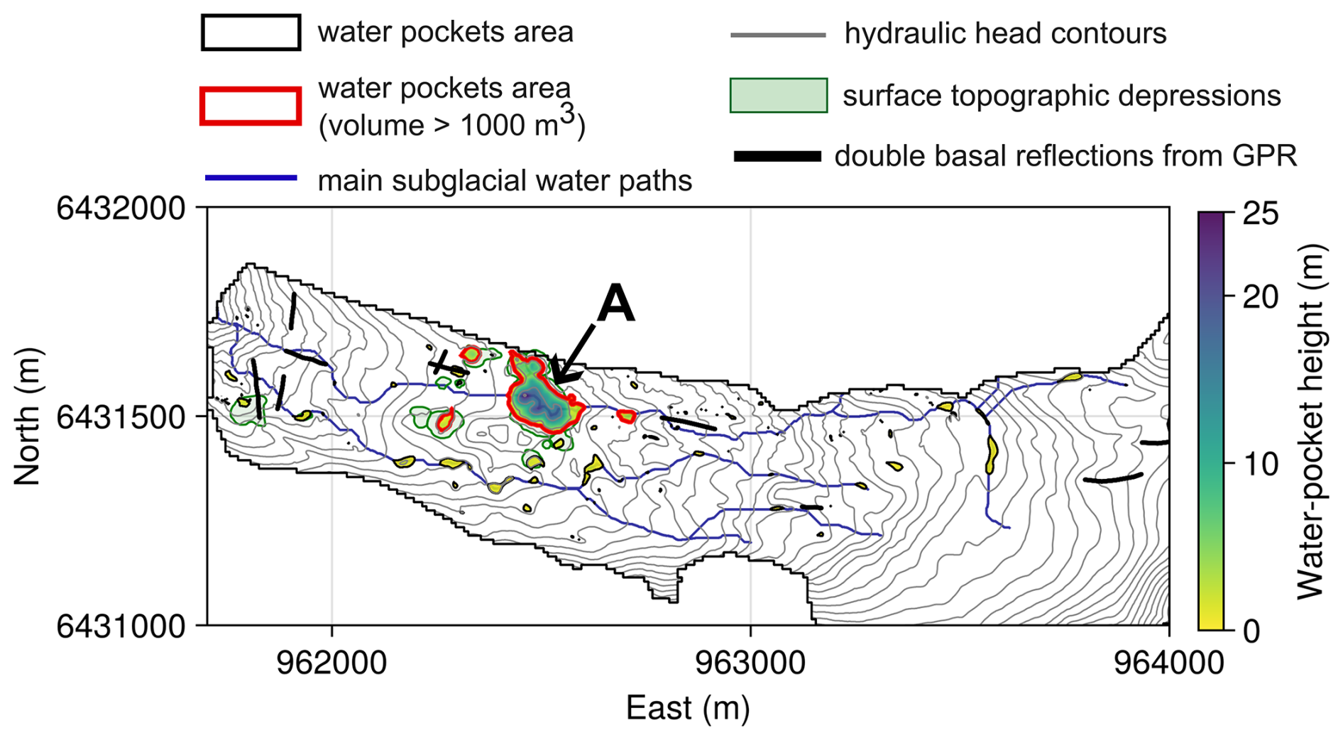
Figure 3 Distributed water-pocket height and main subglacial water paths governed by hydraulic head modelled at Glacier de Bonne Pierre for June 2024 (only the tongue is shown here). The hydraulic head field is shown with thin grey contours at 10 m intervals. Potential water pockets larger than 10³ m³ are outlined in red (in black if smaller). The main surface depressions in the DEM of August 2024 are shown by green shading. The letter A marks both the location of the largest water pocket (148 × 10³ m³) and the location of the supraglacial lake observed in June 2024. Only the subglacial flow paths (blue lines) with an upslope catchment area larger than 10⁵ m² are displayed for visualization (using f = 1 in Eq. 2). Thick black lines show double basal reflections from GPR that suggest the presence of subglacial channels. Glacier outline corresponds to the year 2022.

The lack of surface elevation data in June 2024 prevents the computation of the hydraulic head field at the uppermost part of the glacier. However, the presence of a significant hydraulic barrier at this location is unlikely, as none is observed when using the October 2024 DEM (not shown), and only minor surface elevation changes are expected between June and October of the same year, particularly in the upper part of the glacier. Therefore, the total estimated water volume impounded by hydraulic barriers in June 2024 is assumed to be representative of the whole glacier.

4.3 Stochastic subglacial water routing and water-pocket height

The ensemble-mean of the distributed water-pocket height and ensemble-mean of the upslope catchment areas obtained from 1000 stochastic realizations are shown in Fig. 4. These stochastic realizations were generated to evaluate how perturbations in surface elevation, bedrock elevation, and flotation fraction influence the presence of hydraulic barriers and their associated water-pocket volumes.

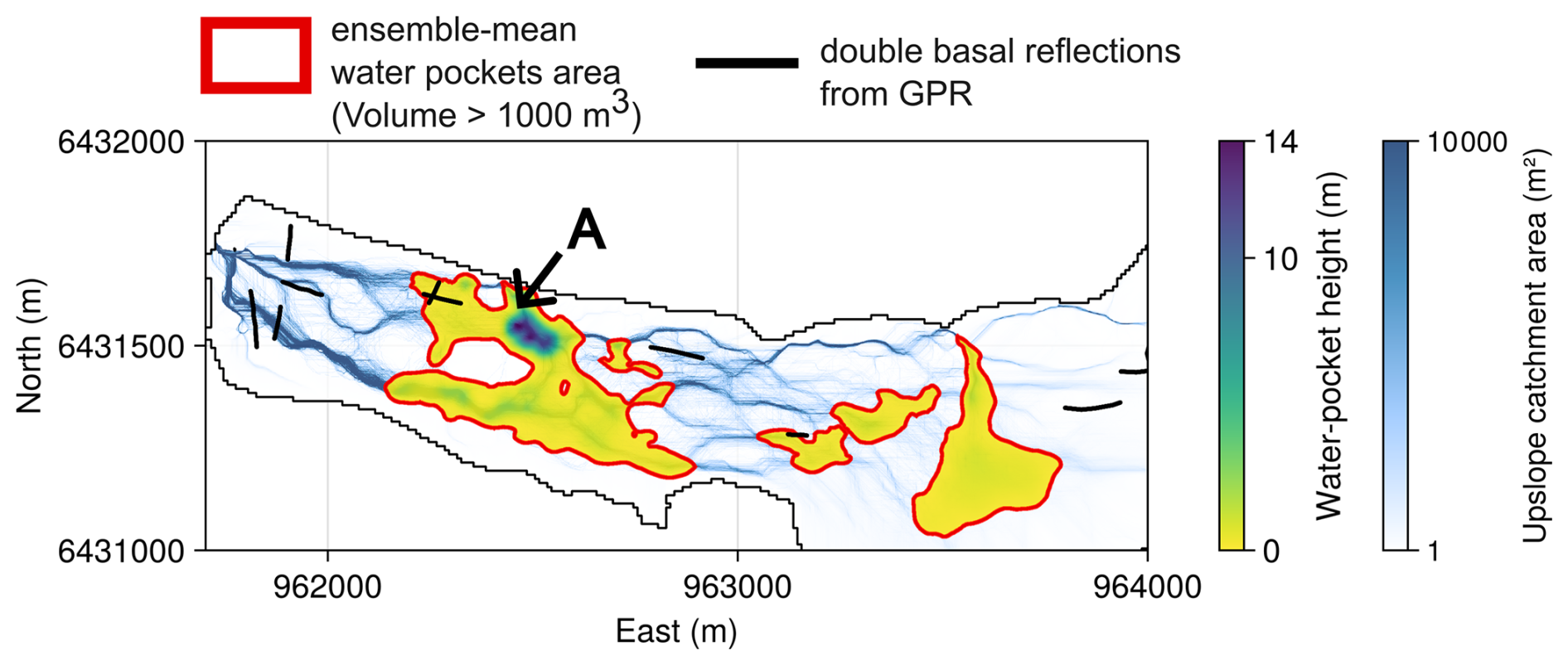
Figure 4 Ensemble-mean water-pocket height and upslope catchment areas from 1000 stochastic realizations of the hydraulic head field at Glacier de Bonne Pierre for June 2024. Only merged outlines of ensemble-mean subglacial water pockets larger than 10³ m³ are shown (in red). The letter A marks the location of the supraglacial lake observed in June 2024. Black lines indicate double basal reflections from GPR interpreted as subglacial channels.

The variability within the ensemble of upslope catchment areas suggests numerous possible re-routings of subglacial water flow paths. This reflects well the sensitivity of subglacial water routing to numerical inputs in Eq. (2) (as shown in Chu et al., 2016; MacKie et al., 2021).

The mean total water-pocket volume of the ensemble realizations, later referred to as the ensemble mean, exceeds the deterministic estimate by 25 % (200 × 10³ m³ vs. 160 × 10³ m³, respectively). The larger volume of water pockets in the ensemble mean is also reflected in a larger mean spatial extent of water pockets compared to the deterministic estimate (Fig. 4 vs. Fig. 3, respectively). This difference comes from the nonlinear response of the hydraulic head field to spatially correlated perturbations in the input variables. Short-scale perturbations in surface elevation, bedrock elevation, or flotation fraction can locally lower the hydraulic head and create new closed depressions, whereas perturbations of opposite sign often do not completely eliminate existing depressions. As a result, positive and negative anomalies do not have symmetric effects on the number and extent of hydraulic barriers. In general, perturbations in the input fields introduce additional local minima in the hydraulic head field, thus creating additional hydraulic barriers and associated water pockets. This effect is particularly evident in areas with low hydraulic gradients, such as flat surface regions and/or bedrock overdeepenings (see Fig. 1a and c, respectively).

The relative contribution of perturbations in surface elevation, bedrock elevation, and flotation fraction to the ensemble variability is discussed in Sect. 5.2.

5 Discussion

5.1 On the possibility of a WPOF at Glacier de Bonne Pierre in June 2024

On 20 June 2024, the main surface depression (Fig. 1a) was filled by a supraglacial lake. Its water volume was estimated at 100 × 10³ m³ based on post-event lake-level marks (Blanc et al., 2024). Because this supraglacial water exerts additional overburden pressure on the possible underlying water pocket, the water pocket corresponding to this topographic depression would be significantly reduced. When using a surface DEM in which the topographic depression is filled with 100 × 10³ m³ of water over a corresponding surface area of 14 000 m² (and converted to distributed overburden ice pressure equivalent), the resulting largest subglacial water pocket has a volume of only 48 × 10³ m³, compared to 148 × 10³ m³ without supraglacial lake filling. Note that, given the bedrock and surface topography, the presence of this supraglacial lake does not produce an additional water pocket impounded by a hydraulic barrier upstream.

In the following, we discuss qualitatively the possible mechanisms that led to the June 2024 outburst, considering hypotheses in which the flood involved additional water stored subglacially, beyond the volume of the supraglacial lake alone.

5.1.1 Scenario 1: Long-term water pocket formation and sudden rupture

In this scenario, a hydraulic barrier beneath the main topographic depression progressively impounds water over multiple years (in A, Fig. 3). Because the supraglacial lake at this location typically lasts only a few weeks each summer since 2016, the subglacial water pocket could continue to grow during the rest of the melt season and remains water-filled through the years, reaching volumes close to the modeled maximum corresponding to a lake-free topographic depression (≈ 148 × 10³ m³). In this conceptual view, the ice roof of the water pocket slowly deforms upward by creep, allowing the reservoir to enlarge over successive years. This slow ice-roof lifting can go undetected from the surface due to the differential spatial patterns of accumulation and ablation, as well as viscous ice flow, which level out the glacier surface.

In June 2024, exceptional rainfall and meltwater inputs caused an unusually rapid rise of the supraglacial lake level, adding significant overburden pressure on the underlying water pocket. This extra load may have triggered a sudden failure of the hydraulic barrier by flotation, leading to the enlargement of subglacial outflow channels (Nye, 1976). This positive feedback between the increasing outflow discharge and subglacial-channel wall melting can release the volume of water stored in the water pocket in a short time.

During the June 2024 glacial outburst, the supraglacial lake can also drain into the same subglacial pathways as the water pocket, in case a newly formed hydraulic connection occurs between the two reservoirs. For instance, such a hydraulic connection can form through hydrofracturing triggered by increased basal water pressure (Stevens et al., 2015), which induces basal slip and/or uplift and promotes tensile stresses within the ice. Crevasses at the base of the supraglacial lake at Glacier de Bonne Pierre were observed a few days after the lake had emptied in 2024. However, it remains unknown whether such a connection between the suggested water pocket and the supraglacial lake existed prior to or during the supraglacial lake drainage. A direct hydraulic connection between the supraglacial lake and the underlying water pocket can trigger hydraulic barrier failure even before its theoretical rupture level is reached, i.e., before basal water pressure equals the ice overburden pressure at the seal. Indeed, once such a connection is established, the hydraulic head at the glacier base is controlled by a water column rather than an ice column, and because water is denser than ice, the same lake surface elevation corresponds to a higher basal water pressure. This additional increase in hydraulic head could have been sufficient to break the hydraulic barrier.

Debris-covered glaciers are prone to such a hydraulic configuration: surface roughness on the order of 10 m induced by debris cover can promote the formation of large surface depressions, in turn leading to both supraglacial lake development and local hydraulic head minima at the glacier bed.

This scenario could, in theory, explain the magnitude of the glacial flood, as the combined release of (i) the supraglacial lake (100 × 10³ m³) and (ii) an additional subglacial water pocket, with an estimated upper bound of ≈ 150 × 10³ m³, would correspond to a total glacial water volume of ≈ 250 × 10³ m³. However, this potential contribution cannot be quantitatively linked to the observed flood, as the hydrological budget of the event cannot be closed due to large uncertainties in discharge estimates caused by instrument failure, intense sediment transport, and channel cross‐section changes during the flood (see Sect. 2). Consequently, the estimated volume of 150 × 10³ m³ should be interpreted as a potential additional subglacial water contribution, rather than as a definitive explanation for the June 2024 flood.

5.1.2 Scenario 2: Spring-event type mechanism

In this scenario, the hydraulic barrier had not led to the accumulation of a large volume of water prior to June 2024, either because the hydraulic barrier was regularly breached during the melt season or because subglacial water input at this location was insufficient to allow significant water accumulation. Instead, we interpret the glacial contribution to the flood as being associated with the exceptional magnitude of water inputs from rain and snowmelt during the event, which likely generated a transient state of very high basal water pressure (possibly locally exceeding the ice overburden pressure). Consequently, the sudden and large water input saturated the inefficient subglacial drainage network, which is typical for the early melt-season. Under such conditions, subglacial water may accumulate temporarily in zones of low hydraulic gradient (as in Fig. 3), forming short-lived but numerous small water-filled cavities (we do not necessarily refer to these water bodies as water pockets due to their small individual sizes).

At this stage, sudden subglacial drainage reorganizations caused by a strong increase in basal water pressure can lead to the development of a connected drainage system that was previously hydraulically isolated. The resulting hydraulic reconnection of water-filled cavities can trigger subglacial floods (e.g., Iken et al., 1996; Kamb, 1987; Warburton and Fenn, 1994; Harper et al., 2005, 2007; Fudge et al., 2008). Such glacial floods are commonly referred to as spring events. Observed spring events have released water volumes comparable to that proposed in Scenario 1, for example at South Tahoma Glacier (USA), where the glacier of approximately 2 km² produced a flood volume of ≈ 300 × 10³ m³ (Walder and Driedger, 1995).

In this view, the flood magnitude in June 2024 is explained not by the rupture of a single, large water pocket, but rather by the sudden drainage of a highly-pressurized and water-saturated subglacial network. The flood caused by the spring event could possibly be amplified by the extra pulse of water input from the supraglacial lake and/or water pocket drainage (as in scenario 1). Comparable behaviour was inferred from field observations at Gornergletscher (≈ 60 km², Switzerland) during the 2004 drainage of an ice-marginal lake with a volume of 4000 × 10³ m³ (Huss et al., 2007). In that case, the integrated flood hydrograph exceeded the lake volume by approximately 800 × 10³ m³, which corresponds to the release of water stored englacially and subglacially prior to the lake drainage. This additional volume was released during the two days following the outburst peak, likely due to increased basal water pressures and a reorganisation of the subglacial drainage network triggered by the lake drainage.

5.1.3 Outlook: observations needed to discriminate between the two scenarios

Distinguishing between these two scenarios would require additional observations. In scenario 1, the volume of subglacial water (≈ 150 × 10³ m³) remains speculative because no direct observations confirm the long‐term persistence of a large water pocket. In particular, the absence of surface deformation features – such as concentric crevasses following water pocket drainage (e.g., Gagliardini et al., 2011; Vincent et al., 2012) – does not support rapid emptying of a large water pocket, although it cannot entirely rule it out. In a spring event (scenario 2), the glacier is expected to temporarily accelerate because distributed high basal water pressures reduce effective pressures (i.e., the difference between ice overburden pressure and water pressure), which possibly leads to bed separation and thus a decrease in basal friction (as observed in Iken and Bindschadler, 1986; Harper et al., 2007; Huss et al., 2007; Fudge et al., 2009; Vincent et al., 2022). The resultant ice uplift from bed separation has been observed to be up to a meter for an alpine glacier (e.g., in Vincent et al., 2022). However, detecting such transient speed-ups and surface uplift would require field observations or high-frequency, high-spatial-resolution imagery, which were not available during the June 2024 event. As a result, observations of glacier motion cannot be used here to discriminate between the two proposed scenarios or to assess their relative likelihood.

Future observations could focus on simultaneous measurements of supraglacial lake level and basal water pressure upstream and downstream of hydraulic barriers to understand the interaction between a supraglacial lake and a potential underlying water pocket. At the glacier scale, high temporal- and spatial-resolution ice surface velocities during melt and rainfall events could help characterize the relationship between basal water pressure variations and subglacial drainage reorganization. In addition, dense seismic arrays deployed at the glacier surface have recently helped resolve spatial and temporal changes in subglacial drainage conditions (Nanni et al., 2021; Guillemot et al., 2024). Combining such observations with ice velocity data would help distinguish between persistent, water-pocket-type reservoirs (scenario 1) and transient spring-event responses to water input (scenario 2).

5.2 Uncertainties in subglacial water routing and total water-pocket volume

Uncertainties in bedrock and surface elevation have often been identified as major sources of error in subglacial water routing models (e.g., Wright et al., 2008; Chu et al., 2016), particularly because bedrock uncertainties often stem from interpolating ice thickness between sparse GPR profiles (MacKie et al., 2021). In this section, we decompose the stochastic ensemble results presented in Sect. 4.3 to isolate and quantify the individual contributions of surface elevation, bedrock elevation, and flotation fraction uncertainties to the total variability in predicted water-pocket volumes. Figure 5a shows the individual contributions of each of these input variable uncertainties to the spread of water-pocket volumes of the stochastic ensemble. Their individual contributions are obtained by perturbing only one field at a time across the 1000 Monte Carlo realizations ($z_{\mathrm{s}}^{*}$, $z_{\mathrm{b}}^{*}$, or f^* in Eq. (5)) and calculating the corresponding hydraulic head (Eq. 2). Results are summarized in Table 1.

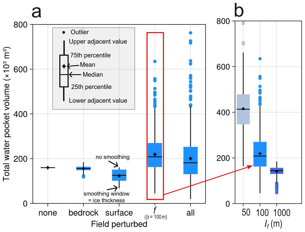
Figure 5 Boxplots of total water-pocket volumes across stochastic realizations for different uncertainty configurations. (a) Sensitivity to individual perturbations: a deterministic case with no perturbed input fields (“none”), bedrock elevation perturbed only, surface DEM perturbed (smoothed) only, flotation fraction (f) perturbed only using l_f = 100 m, and all perturbations combined (“all”). (b) Sensitivity to the spatial correlation length of flotation fraction perturbations, shown for l_f = 50 m, 100 m (as in panel a), and 1000 m. Boxes indicate the interquartile range, with medians shown as horizontal lines and means as crosses. Whiskers extend to 1.5 times the interquartile range, and circles denote outliers.

Table 1 Summary of deterministic and stochastic estimates of total subglacial water-pocket volume at Glacier de Bonne Pierre as of June 2024. Stochastic values are expressed as ensemble mean ± standard deviation (see Fig. 5 for the full distribution of total water-pocket volumes). Surface DEM smoothing uses a moving-average boxcar filter with window size equal to 0 %–100 % of local ice thickness. The flotation fraction f varies within the range 0.9–1.1, representing subglacial water pressures from below to above ice overburden pressure, and l_f denotes the spatial correlation length of the random field used to represent uncertainty in f. Note that these volumes correspond to maximum potential volumes of water pocket for each configuration and could not be evaluated because of the lack of in situ observations.

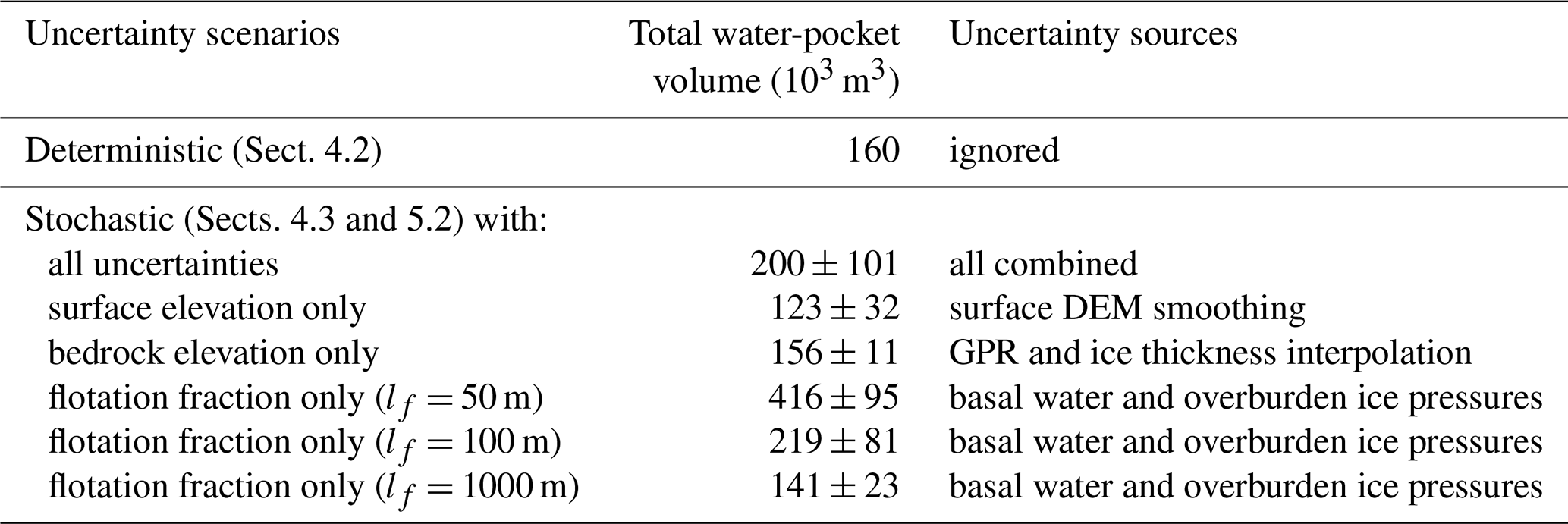
Bedrock elevation uncertainties have a relatively small influence on the resultant total water-pocket volume, although the maximum uncertainty can locally reach up to 24 m (see Fig. 2d). The total water-pocket volume of the ensemble under bedrock uncertainties is 156 × 10³ ± 11 × 10³ m³.

The total volume of water pockets within the surface uncertainties is 123 × 10³ ± 32 × 10³ m³. This variability reflects the range of smoothing windows applied to the surface DEM (from 161 × 10³ m³ without smoothing to 67 × 10³ m³ for a smoothing window equal to 100 % of the local ice thickness). Increasing the smoothing window progressively reduces the resulting total water-pocket volume, as this smooths surface depressions and reduces local variations in the subglacial hydraulic head field. The strong sensitivity of the hydraulic head field to surface smoothing highlights a potential source of error for other studies, where surface DEMs may not be reconstructed as accurately as in this study (i.e., from high-resolution LiDAR), or more generally when surface smoothing is applied based on arbitrary choices.

Although glacier surface elevation is well reconstructed by LiDAR measurements, the ice overburden pressure and the basal stress field – which control the hydraulic head – are subject to additional uncertainty. In particular, debris cover is not explicitly accounted for in surface elevation, although it is widely present at the tongue of Glacier de Bonne Pierre. Debris has a density approximately three times higher than the density of ice. However, neglecting debris thickness in the calculation of the hydraulic head is reasonable because field observations at Bonne Pierre tongue suggest that debris thickness rarely exceeds a few decimetres (Antoine Blanc, personal communication). Note also that possible thicker debris in the central part of the glacier can be represented through variations in the flotation factor (see below), which indirectly reflect changes in ice overburden pressure and thus ice thickness (see Eq. 2).

Relative variability in the flotation fraction f of only ± 10 % leads to both the largest total water volumes and the largest spread across realizations (Fig. 5a).

Here, spatial variability in f is used to capture the contribution to the hydraulic gradient due to the unknown spatial variability in basal water pressure (see Eq. 2). The arbitrary range of f values chosen in this study spans a limited spectrum of the values encountered in reality: f = 0.9 reflects relatively low water pressure where the subglacial system likely channelizes, and f = 1.1 represents a pressurized drainage system with water pressure larger than ice overburden pressure, which may occur when subglacial water input exceeds outflow. Such conditions are considered realistic prior to and during the June 2024 flood at La Bérarde – at least locally – given the high water input from rainfall and snowmelt in the glacier catchment. Values of f > 1 have been locally observed for short periods in borehole water-level measurements (Harper et al., 2005; Huss et al., 2007; De Fleurian et al., 2016; Rada and Schoof, 2018) and have been reproduced in physically-based models of the subglacial drainage system (Werder et al., 2013). Under these overpressurized conditions, water could spread across the bed through linked subglacial cavities (e.g., Kamb, 1987) and/or flow upward through moulins or crevasses connected to the subglacial drainage system, eventually causing overflow at the surface. However, note that the quantity of interest to the routing model is the gradient of the hydraulic head, and therefore a value of f > 1 does not necessarily translate into a statement that the water pressure is greater than the ice pressure; rather, it states that the gradient downstream of a f > 1 area is larger than what the Shreve potential (f = 1) would predict.

Variations in basal water pressure have been identified as a key control on subglacial water routing (Chu et al., 2016). However, to our knowledge, spatial correlation lengths have not previously been assessed in steady-state subglacial water-routing models to explicitly represent such variability in basal water pressure. Here, we show that the spatial correlation length l_f assigned to the perturbations in f strongly controls the resulting total water volume (Fig. 5b). A short correlation length (l_f = 50 m) generates numerous small, localized anomalies in the hydraulic head field and produces many additional water pockets, resulting in a larger total volume (419 × 10³ ± 94 × 10³ m³) than for longer l_f. An intermediate correlation lengths (l_f = 100 m) produces fewer hydraulic barriers, with a volume still exceeding the deterministic case (215 × 10³ ± 79 × 10³ m³ vs. 160 × 10³ m³). The numerical reasons for these differences between deterministic and stochastic estimates were discussed in Sect. 4.2. A longer correlation length (l_f = 1000 m) creates broad perturbations of the hydraulic field; therefore, it reduces the number of independent hydraulic barriers and decreases the total stored volume (140 × 10³ ± 22 × 10³ m³).

The range of correlation lengths explored here is arbitrary but still motivated by in situ observations of basal water pressure variability. For instance, borehole observations at Bench Glacier (Alaska) showed that water-level fluctuations became uncorrelated beyond a typical distance of 10 m in the cross-glacier direction, whereas typical down-glacier correlation lengths were estimated at typically 100 m (Fudge et al., 2008). Although these estimates apply to a specific glacier and season, they provide a reasonable order of magnitude for our study.

Overall, these stochastic simulations illustrate how sensitive subglacial routing is to uncertain spatial variations in basal water pressure. Note that while basal water pressure also varies over short timescales (e.g., Rada and Schoof, 2018), capturing such temporal dynamics goes beyond the steady-state framework adopted in this study.

6 Conclusions

In June 2024, an unprecedented flood of the Etançons river (Ecrins, France) caused the near complete destruction of the village of La Bérarde. Post-event analyses showed that the timing of the flood could not be explained by rainfall and snowmelt alone, suggesting an additional glacial contribution from Glacier de Bonne Pierre located upstream of La Bérarde. Using surface and bedrock elevations as input to a steady-state subglacial water routing algorithm, we provided an estimate of the maximum potential volume of subglacial water pockets that could have been impounded by hydraulic barriers, i.e., in minima of the hydraulic head field. We found that such hydraulic barriers at the glacier tongue could have, in theory, impounded 160 × 10³ m³ of water in June 2024, with the largest water pocket (148 × 10³ m³) located beneath the main surface depression that temporarily hosts a supraglacial lake during summer. In addition to the drainage of this supraglacial lake (≈ 100 × 10³ m³), this potential subglacial water storage could have contributed to the flood magnitude. However, the lack of direct observations of water pockets and the steady-state nature of our numerical approach prevent a definitive attribution of the flood mechanism. In particular, our results do not rule out a spring-event-type mechanism involving the rapid drainage of a highly pressurized and saturated subglacial drainage network.

Our uncertainty analysis showed that bedrock elevation uncertainties have a relatively small impact on the estimated total water-pocket volume (± 11 × 10³ m³), while surface uncertainties – represented by the range of smoothing windows applied to the surface DEM – have a larger impact (±32 × 10³ m³). Variations in the flotation fraction f, used here as a proxy for unresolved spatial variability in basal water pressure, dominate the uncertainty. Variations in f of ±10 % can lead to total water-pocket volume of several 100 × 10³ m³, with strong sensitivity to the assumed spatial correlation length, a parameter that remains poorly constrained due to the hidden nature of the subglacial system.

From a hazard perspective, debris-covered glaciers hosting large surface depressions – such as at Glacier de Bonne Pierre – deserve focused monitoring, as these settings may favour the co-occurrence of supraglacial lakes and subglacial water pockets by hydraulic barriers, with both reservoirs potentially reaching rupture conditions during extreme melt or rainfall events.

Appendix A: Uncertainties

Uncertainties in surface elevation, bedrock elevation, and flotation fraction directly affect the calculation of the hydraulic head (Eq. 2) and the resulting total volume of water pockets (Eq. 4). Here, we quantify the magnitude and spatial correlation of these uncertainties, which are used to generate random fields and provide the input for the stochastic realizations of the hydraulic head field (Sect. 3.6).

A1 Uncertainties in bedrock elevation z_b

The point-specific uncertainty in bedrock elevation, u_bed(x,y), represents the standard uncertainty at each location (x,y) in the distributed bedrock topography. It results from three independent sources: the GPR measurement uncertainty u_GPR(x,y), the interpolation uncertainty from mass-conservation methods u_int(x,y), and the LiDAR surface elevation uncertainty u_LiDAR(x,y). Assuming these three sources are independent, the combined uncertainty is obtained by summing them in quadrature:

$$\begin{array}{}\text{(A1)}& \begin{array}{rl}& u_{\mathrm{bed}}(x,y)\\ & =\sqrt{\left(u_{\mathrm{GPR}}\right(x,y){)}^{\mathrm{2}}+(u_{\mathrm{int}}(x,y){)}^{\mathrm{2}}+\left(u_{\mathrm{LiDAR}}\right(x,y){)}^{\mathrm{2}}}.\end{array}\end{array}$$

The contribution from LiDAR surface elevation, u_LiDAR(x,y), to the total bedrock elevation uncertainty is negligible (typically a few millimetres to centimetres) and is therefore ignored here.

The GPR uncertainty range represents the confidence interval with which the bedrock interface is manually picked in the radar profiles. We adopt a conservative value of ±5 m based on the profile-quality analysis of (Santin et al., 2025), which is consistent with the average picking uncertainty reported by Grab et al. (2021). The pixel-specific contribution u_GPR(x,y) is obtained by repeating the ice-thickness inversion with GlaTE twice, once using the maximum and once the minimum ice thickness consistent with the GPR picking range.

The interpolation uncertainty u_int(x,y) arises from the limited spatial coverage of GPR measurements and the need to interpolate ice thickness between profiles. In this study, it represents the dominant component of bedrock elevation uncertainty, particularly in areas far from GPR observations. u_int(x,y) is quantified using a spatial leave-out experiment known as “leave-ball-out” or “leave-block-out” (Le Rest et al., 2014). In this experiment, GPR thickness measurements within a radius around randomly selected locations are temporarily removed. The mass-conservation inversion is then applied, and the resulting bedrock elevations are differenced to the original GPR elevations at the removed locations, which yield bedrock elevation errors. We used a 500 m radius for the leave-ball-out, corresponding to the maximum interpolation distance between GPR points, and performed 20 simulations with different random locations.

The per-pixel variability of errors (heteroscedasticity) and spatial correlation of errors were estimated following the framework of Hugonnet et al. (2022) on the leave-ball-out errors. First, we studied the variability in uncertainty magnitude along two variables: the horizontal distance to the nearest GPR measurement, and the ice thickness. For each variable, we estimated the uncertainty by computing the standard deviation of leave-ball-out errors in binned categories. We found that the horizontal distance d explained all the variability in uncertainty magnitude, and modelled it by a linear fit of the binned estimates (Fig. A1a). In our case, the 1-σ bedrock uncertainty (m) increases approximately linearly with distance d (m) as follows:

$$\begin{array}{}\text{(A2)}& {\mathit{\sigma }}_{\mathrm{err}}\left(d\right)=\mathrm{0.0411}d+\mathrm{13.35}.\end{array}$$

The spatial correlation of the errors was characterized using variography (Cressie, 2015). For each simulation, we estimated an empirical variogram using the leave-ball-out errors standardized by their variability σ_err(d) (i.e. divided into standard scores with unit variance). We then aggregated the variograms of individual simulations by a weighted mean, and fit a Gaussian model (Fig. A1b). The fitted Gaussian variogram model has an effective range parameter R_bed = 247.4 m, defined as follows:

$$\begin{array}{}\text{(A3)}& {\mathit{\rho }}_{\mathrm{SGS}}\left(h\right)=\exp \left(-{\displaystyle \frac{\mathrm{4}{h}^{\mathrm{2}}}{R_{\mathrm{bed}}^{\mathrm{2}}}}\right).\end{array}$$

We note that, due to the different formulation of the range for a Gaussian model in WWFS, we convert the range to ≈ 175 m. This range parameter thus characterizes the spatial correlation length of the uncertainty in bedrock elevation u_bed(x,y), while its local magnitude is given by Eq. (A1).

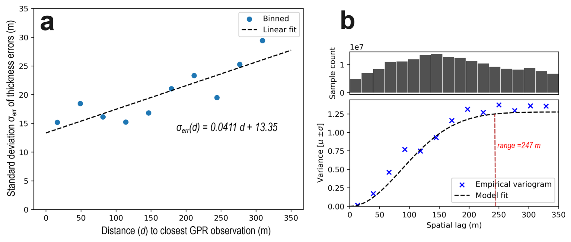
Figure A1 (a) Linear relation between the standard deviation error of ice thickness and distance to the closest GPR observation. (b) Spatial variogram of standardized ice thickness differences. The empirical variogram is modelled by a Gaussian model.

A2 Uncertainties in the flotation fraction f

The flotation fraction f, i.e., the ratio of water pressure to ice overburden pressure, plays an important role in the calculation of the hydraulic potential used to route subglacial water (Eq. 2). It is classically set to one (Shreve, 1972). However, this ratio varies in space and time (e.g., Iken et al., 1996; Harper et al., 2005; Lefeuvre et al., 2015; Rada and Schoof, 2018).

In the absence of direct observations of subglacial water pressure at Glacier de Bonne Pierre, the treatment of f in this framework should be interpreted as a sensitivity analysis rather than a strict quantification of uncertainty. The lower bound f = 0 corresponds to basal water at atmospheric pressure, i.e. when the water is solely driven by the gravity potential in an open air channel. This case is not considered in this study. f < 1 reflects water pressures below flotation. This reflects the possibility of water to overcome hydraulic barriers without the need to reach ice overburden pressure (e.g., if water can enter reminiscence of channels or cracks). This is associated with efficient drainage systems. f can locally exceed one when the water is at a pressure exceeding the ice overburden pressure. This may happen when a large input of meltwater or rain enters and saturates the glacier drainage system (e.g., in Bartholomaus et al., 2008; Harper et al., 2005, 2007; Rada and Schoof, 2018).

We arbitrarily varied f across the glacier domain within the range 0.9–1.1. Note that variations of f in the range 0.6–1.11 and 0.8–1.1 have been applied in steady-state subglacial water routing models by Chu et al. (2016) and Bowling et al. (2025), respectively. However, these studies assumed a spatially uniform (i.e., fully correlated) value of f, which does not account for the spatial variability expected in this parameter.

The spatial correlation length, l_f, defines the typical scale over which pressure anomalies remain correlated; beyond this distance, variations in water pressure are assumed to be independent. We assume a relatively short correlation length – l_f = 100 m – to reflect the transient and weakly connected nature of the subglacial drainage system, where non-communicating flow components likely coexist (see subglacial water pressure records in Hubbard et al., 1995; Fountain and Walder, 1998; Fudge et al., 2008; Lefeuvre et al., 2015; Rada and Schoof, 2018). We acknowledge that our choice for l_f is arbitrary due to the limited knowledge of the subglacial drainage network at Glacier de Bonne Pierre, and we assess its sensitivity in Sect. 5.2.