Probabilistic flood hazard mapping for dike-breach floods via graph neural networks

Flood hazard maps are essential for protection and emergency plans, yet their probabilistic application is constrained by the computational cost of numerical models. Deep learning surrogates can provide orders of magnitude faster predictions, but their use for uncertainty quantification in realistic settings and their ability to incorporate hydraulic structures remain largely unexplored. Studying deep learning surrogates for probabilistic flood maps is non-trivial because of the lack of reference ground-truth data that might lead to misleading confidence in predictions. Moreover, hydraulic structures are challenging to include due to their generally unidimensional nature. In this work, we investigate the use of deep learning surrogates for realistic, large-scale flood simulations in case studies with hydraulic structures under diverse boundary conditions. To this end, we employ the multi-scale shallow-water-equations graph neural network (mSWE-GNN) that enjoys transferability to different boundary conditions and locations and whose graph-based architecture allows to represent structures such as canals, underpasses, and elevated elements as inputs. To address the lack of reference ground-truth data, we further introduce the average relative mass error (ARME), a mass-conservation-based criterion that helps identify physically plausible simulations. We applied the model on dike ring 41 in the Netherlands, generating probabilistic flood maps that account for uncertainties in breach location and breach outflow hydrographs. The model was trained on 30 simulations, generated with Delft3D, and evaluated against unseen benchmark simulations from the Dutch national flood catalogue, achieving a critical success index (CSI) of 73.6 % while running 10 000 times faster than the numerical simulator. The proposed ARME is negatively correlated with the CSI, with a Spearman correlation coefficient of −0.7, making it a useful indicator of simulation plausibility when evaluating unseen case studies. We obtained probabilistic flood maps by running 10 000 different flooding scenarios on a computational mesh of 180 000 cells in approximately 10 h, with about half of the simulations classified as plausible based on the mass-conservation check. This framework offers a practical tool for rapid probabilistic flood hazard assessment and a way to prioritize detailed physical simulations, supporting more efficient and robust flood risk management.

1 Introduction

Probabilistic flood hazard maps quantify the likelihood of different flooding scenarios based on their uncertainty. Unlike deterministic approaches, which compute a single estimate of water depth, extent, and intensity for a specific return period (Dottori et al., 2021), probabilistic maps explicitly account for uncertainties in flood drivers and system responses. These uncertainties may stem from factors such as river discharge hydrographs (Savage et al., 2016), maximum water levels (de Moel et al., 2014), roughness coefficients (Hall et al., 2011; Savage et al., 2016), or flood duration (de Moel et al., 2014). Further uncertainties can appear when quantifying the statistical fit of a model with limited data and treating metrics as deterministic (Huang and Merwade, 2024). As a result, probabilistic approaches avoid underestimating risks that happen with deterministic methods (Hall and Solomatine, 2008; Savage et al., 2016).

Building probabilistic hazard maps remains challenging as the number of uncertain variables can be large, particularly for dike breaching, where additional geotechnical properties must be considered. Uncertainties include breach location (D'Oria and Maranzoni, 2019; Westerhof et al., 2023), breach width (Mazzoleni et al., 2014; de Moel et al., 2014), breach development time (Apel et al., 2006; Ferrari et al., 2020), failure time (D'Oria and Maranzoni, 2019), and failure mechanism (D'Oria and Maranzoni, 2019; Mazzoleni et al., 2014). Estimating output uncertainty may require up to hundreds of thousands of simulations, making standard numerical flood models computationally prohibitive unless using large high-performance clusters (Gibbons et al., 2020). Simplified hydraulic models have been explored to reduce costs, but they often provide low accuracy or limited outputs, such as only final water levels (Apel et al., 2006; de Moel et al., 2014).

Recent years have seen a rapid expansion of deep learning (DL) surrogate models as fast and accurate alternatives to traditional numerical models (Bentivoglio et al., 2022). Most studies focus on predicting maximum water depth maps (e.g., Gao et al., 2024; Liao et al., 2023; Guo et al., 2020) or predicting the full spatio-temporal evolution of floods (e.g., Pianforini et al., 2025; Cao et al., 2024; Song et al., 2025; Burrichter et al., 2023) while generalizing on different boundary conditions, such as rainfall or river discharges. In terms of types of floods, most works investigate pluvial floods, mainly driven by rainfall (Wang et al., 2024; Shao et al., 2024), while few others cover coastal (Xu and Gao, 2024), river (Pianforini et al., 2025), and dike-breach floods (Wei et al., 2024). Despite achieving good accuracy and speed, these models focus on a single domain, meaning that they require retraining in unseen case studies or even placement of localised boundary conditions (contrary to, for example, spatially distributed rainfall), ultimately limiting their practical use. To address this limitation, several studies have addressed the transferability of DL models to unseen case studies and boundary conditions, with convolutional-based models (do Lago et al., 2023; Guo et al., 2022; Cache et al., 2024) and graph-based ones (Bentivoglio et al., 2023, 2025; Kazadi et al., 2024). In particular, graph-based models showed high transferability to boundary conditions and locations and a stronger link with physics.

However, DL models are typically validated on a limited range of simulations, leaving their reliability in truly unseen scenarios uncertain unless additional reference simulations are available. They also cannot accommodate hydraulic structures (e.g., canals, elevated roads, and underpasses), whose complex geometries strongly affect flow. To achieve probabilistic flood hazard maps in realistic settings, DL models require two properties. First, they need to account for hydraulic structures rather than only via digital elevation models. This is challenging because these small-scale structures, though minor in size, can significantly alter flood behaviour. Second, they require a validation procedure that works without ground-truth data, as the latter is often unavailable.

Tackling the above challenges, this work advances probabilistic flood modelling by using a deep learning surrogate for real-world probabilistic dike-breach flood hazard mapping. Our work provides four key contributions.

• First, we integrate hydraulic structures such as canals and elevated elements into deep learning models as inputs, overcoming a key limitation of existing surrogates. Specifically, we consider the mSWE-GNN from Bentivoglio et al. (2025), as it supports time-varying boundary conditions, ensures physical consistency, and is the only model achieving demonstrable generalizability to unseen boundary conditions as well as unseen boundary locations, a key requirement for probabilistic flood mapping. The graph nature of the model allows integrating hydraulic structures by explicitly representing them as additional edge or node features and by adapting the computational mesh to them, enabling the network to learn how such structures influence flow propagation.

• Second, we introduce an average relative mass error (ARME) metric based on mass conservation to assess the validity of surrogate predictions, particularly under unseen scenarios where reference solutions are unavailable. The ARME is negatively correlated with the critical success index (CSI), making it a reliable proxy for validating predictions.

• Third, we validate our approach on a large-scale realistic low-lying area in the Netherlands protected by flood defences and with a wide coverage of hydraulic structures, with approximately 180 000 computational cells. We considered uncertainty in breach outflow hydrograph and breach location, influenced by both river water levels and dike strength. We train our model on 30 numerical simulations and compare our results against a catalogue of Dutch national flood hazard maps (VNK) (Rijkswaterstaat, 2016) for multiple breach locations and return periods, obtaining a CSI of 73.6 % while running 10 000 times faster than the numerical simulator.

• Lastly, we computed probabilistic flood maps over 10 000 different flooding scenarios in about 10 h on a single GPU and found that half of the simulations have a plausible mass conservation according to the ARME metric. We also analysed the uncertainty in flood arrival times and maximum water depths for a test case, comparing an ensemble of predictions against a single deterministic estimate, showing that the ensemble members are more accurate than the single case.

This work provides a practical, validated pathway for integrating deep learning surrogates into operational probabilistic flood hazard mapping and risk assessment.

The rest of the paper is structured as follows: Sect. 2 describes the proposed approach for incorporating hydraulic structures into the mSWE-GNN model, the mass-conservation-based validation methodology, and the procedure for generating probabilistic flood maps. Section 3 outlines the experimental set-up and case study. Section 4 presents model validation, a large-scale analysis of the ARME across 10 000 scenarios, the generation of probabilistic flood maps for both the large-scale analysis and a test condition, and an ablation study evaluating the impact of incorporating hydraulic structures. Finally, Sect. 5 summarizes the main findings and their implications.

2 Methodology

We designed a graph-based surrogate model for dike breach flood modelling that includes hydraulic structures as inputs (Fig. 1a). We trained and tested our model on a dataset of numerical simulations, auto-regressively predicting water depths and unit discharges over time. We analysed the uncertainty in flood hazard mapping considering an ensemble of breach locations and outflow discharges. To improve prediction reliability when no ground-truth simulations exist, we introduced a verification procedure based on mass conservation (Fig. 1e). Using the plausible simulations, we then estimated probabilistic hazard maps.

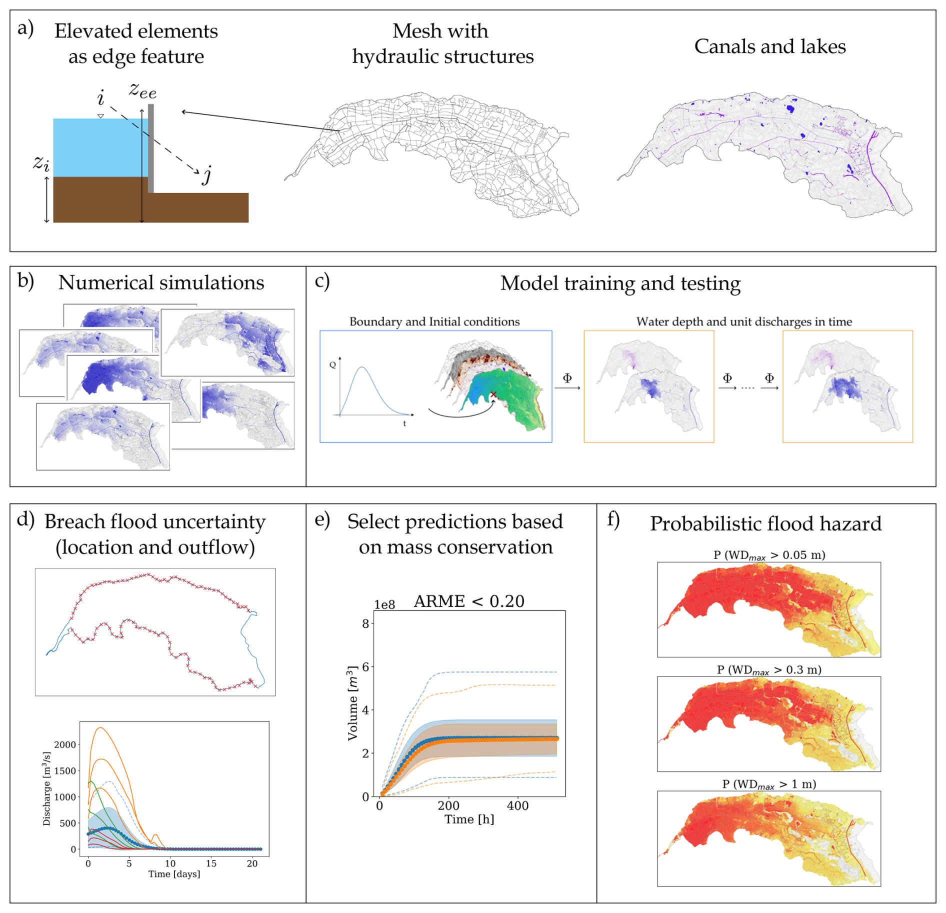
Figure 1 Proposed methodology for probabilistic dike-breach flood hazard mapping. (a) Hydraulic structures such as elevated elements and canals are inputs. The difference between elevated elements (z_ee) and the terrain (z_i) is treated as an additional edge feature. (b) The model is trained and tested on a dataset of numerical simulations. (c) The network Φ receives node features (topography, roughness, water bodies, and initial hydraulic states) and edge features (mesh connectivity and elevation differences at hydraulic structures). It predicts water depths and unit discharges at the next time step, repeating this process auto-regressively using the predicted outputs as a new initial condition to simulate the full spatio-temporal flood dynamics. Boundary conditions are enforced through ghost cells. The architecture operates across multiple mesh resolutions, with node and edge features defined at each scale. A zoom-out detail is shown in Fig. 2. (d) Flood uncertainty, represented via 10 000 combinations of breach locations and outflow discharges. (e) Plausible simulations are selected based on the average relative mass error computed against the input inflows. (f) Selected simulations provide conditional probabilities of flooding, assuming the same probability of occurrence for each scenario.

First, this section describes the surrogate flood model and its adaptation to include hydraulic structures and water bodies (Sect. 2.1). Next, we introduce the mass-conservation-based metric (Sect. 2.2). Finally, we detail the procedure to create probabilistic flood maps that account for input uncertainties (Sect. 2.3).

2.1 Multi-scale hydraulic graph neural networks

2.1.1 Model

The multi-scale hydraulic graph neural network (mSWE-GNN) is a graph-based deep learning architecture that models the two-dimensional spatio-temporal evolution of floods (Bentivoglio et al., 2025). It treats the cells of a computational mesh as nodes in a graph and connects neighbouring cells with edges. It learns flood spreading by combining local flow propagation with a series of graph neural network (GNN) layers at different spatial resolutions (Fig. 2). Each GNN computation is based on the finite volume approximation of the shallow water equations, enforcing a physical bias in the propagation rule (Bentivoglio et al., 2023). The model takes static features representing topography, terrain roughness, and domain connectivity at different resolutions, and dynamic features representing hydraulic variables at time t. It processes these inputs with a U-shaped architecture that applies GNNs at multiple scales and combines them through skip connections. The model predicts the hydraulic variables, water depth h [m] and the absolute value of unit discharge $\left|\mathit{q}\right|$ [m² s⁻¹], at the next time step t+1, at the finest available resolution. Ghost cells at the domain boundary enforce known boundary conditions.

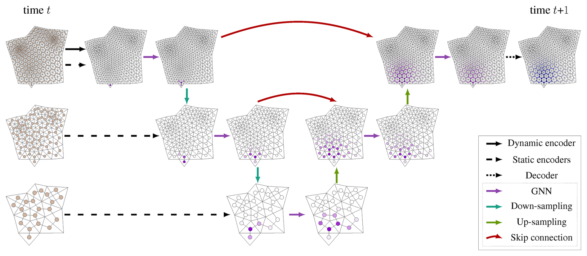
Figure 2 The mSWE-GNN model (Bentivoglio et al., 2025). The inputs are node and edge features defined on multiple mesh resolutions at time t and the predictions are water depths and discharges at the next time step t+1. The multi-scale architecture consists of three encoders, which create high-dimensional embeddings of the inputs; a U-Net-like processor, which consists of a sequence of graph neural network layers followed by down-sampling and up-sampling operators; and a decoder, which converts node embeddings into hydraulic variables.

The mSWE-GNN uses an explicit numerical scheme to auto-regressively predict hydraulic variables at time t+1 as

$$\begin{array}{}\text{(1)}& {\widehat{\mathbf{U}}}^{t+\mathrm{1}}=\mathit{\sigma }\left({\mathbf{U}}^t+\mathrm{\Phi }({\mathbf{X}}_{\mathrm{s}},{\mathbf{U}}^{t-p:t},\mathcal{E})\right),\end{array}$$

where ${\widehat{\mathbf{U}}}^{t+\mathrm{1}}$ is the predicted hydraulic variables, U^t are the hydraulic variables (water depth [m] and unit discharge [m² s⁻¹]) at time t, Φ(⋅) is the model for a fixed time step, X_s are static node features, ${\mathbf{U}}^{t-p:t}$ are dynamic node features for time steps t−p to t, with p indicating the number of previous times steps given as input, σ is a rectified linear unit (ReLU) used for guaranteeing positive hydraulic variables, and 𝓔 are edge features. The node features are divided into static and dynamic to isolate the hydraulic variables so that cells without any water will have dynamic node features equal to zero: this concept is used in the SWE-GNN layers to preserve physical consistency in water propagation (Bentivoglio et al., 2023). Node and edge features also neglect coordinates and orientation-dependant values to ensure translational and rotational invariance.

2.1.2 Including hydraulic structures

We model hydraulic structures, such as canals, elevated roads, and underpasses, by modifying the computational meshes, edge features, and node features. These modifications provide more physical inductive bias to the model but do not affect the propagation rule in Eq. (1).

• Canals. We create longitudinal polygonal elements in the coarse mesh resolutions to represent canal segments (see Fig. 1a). This helps the model recognize their distinct propagation speeds, similarly to how 1D elements work in numerical models. The longitudinal elements are not needed in the finest scale if the mesh cells are already small enough to correctly separate canals from the terrain. We add binary node features to indicate the presence of a canal, using one-hot encoded vectors that are one for canal cells and zero otherwise.

• Water bodies. We create polygonal elements in the coarse mesh resolutions to represent water bodies, such as ponds and lakes (see Fig. 7a–c). This helps the model recognize that they are not source points. Similarly to canals, the polygonal elements are not needed in the finest mesh if it is detailed enough to separate water bodies from dry terrain. As for canals, we add binary node features to indicate the presence of a lake, using one-hot encoded vectors that are one for lake cells and zero otherwise.

• Elevated roads. We model elevated roads and similar one-dimensional elements with a marked elevation difference from the surrounding topography via edge features. We identify graph edges that intersect these structures using geospatial intersection and assign each directed edge (from node i to node j) a value equal to the height difference from the source node i to the elevated element z_ee, i.e., z_ee−z_i, as shown in Fig. 3. This feature increases with elevation difference, guiding the model to recognize that water can only cross the structure once the water level surpasses its height, and thus it is more difficult for flow to occur from that side. We also modify the coarsest mesh to create polygonal elements that follow the shape of elevated roads and encompass areas partially or fully enclosed by elevated features, similarly to Lhomme et al. (2008). This helps the model recognize their presence and understand that they may block water flow locally.

• Underpasses. Underpasses are represented by lowering the elevation at the underpass location, effectively creating a hole that allows water to flow beneath elevated roads. This ensures the model can learn that water is not fully blocked by elevated structures.

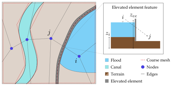
Figure 3 Left: Example coarse mesh creation process around canals and elevated roads. The mesh elements are adapted to fit the shape of these hydraulic objects. Right: schematization of how elevated elements are added as edge features. For each edge (i,j) that intersects an elevated element, we determine the feature as the difference in elevation from that of the element (z_ee) to that of the source node i (z_i).

2.1.3 Model inputs

The inputs consist of static and dynamic node features and edge features extracted from the mesh and its variables.

• The static node features for the ith finite volume are ${\mathit{x}}_{\text{si}}=(a_i,e_i,r_i,w_i^t,c_i,l_i)$, where a_i is its area, e_i its elevation, r_i its roughness coefficient, $w_i^t$ its water level, given by the sum of the elevation and water depth at time t, and c_i and l_i are binary masks that indicate whether a node represents a canal or a lake, respectively. Following Bentivoglio et al. (2023), we treat the water level $w_i^t$ as a static rather than a dynamic feature. Although it is updated over time, it retains non-zero values even in dry cells due to the elevation term, meaning that including it among the dynamic inputs would violate the hydraulic-preservation criterion of the SWE-GNN layer.

• The dynamic node features ${\mathit{x}}_{\text{di}}={\mathit{u}}_i^{t-p:t}=({\mathit{u}}_i^{t-p},\mathrm{\dots },{\mathit{u}}_i^{t-\mathrm{1}},{\mathit{u}}_i^t)$, represent the initial and previous states of the hydraulic variables, where ${\mathit{u}}_i^t=(h_i^t,|q{|}_i^t)$ and h refers to water depths [m] and $\left|q\right|$ to the unit discharges [m² s⁻¹], respectively.

• The edge features are ${\mathit{\epsilon }}_{ij}=(l_{ij},z_{\text{ie}})$, where l_ij is the distance between the centres of nodes i and j and z_ie is the elevation difference between the elevated element z_ee and that of the source node z_i, that is z_ee−z_i, which is set to zero in the case of no structure.

As in Bentivoglio et al. (2025), all inputs are independent of the coordinate values and mesh orientation, as it makes the model more generalizable and less prone to overfitting on a specific case study. Similarly, edge features depend only on the connectivity between two nodes and not on their orientation.

2.1.4 Training

We train the mSWE-GNN end-to-end using flood simulations as training data. We apply a multi-step-ahead loss and a curriculum learning strategy to minimize error accumulation over time (Bentivoglio et al., 2023):

$$\begin{array}{}\text{(2)}& \mathcal{L}={\displaystyle \frac{\mathrm{1}}{HO}}\sum _{\mathit{\tau }=\mathrm{1}}^H\sum _{o=\mathrm{1}}^O{\mathit{\gamma }}_o\left|\right|{\widehat{\mathit{u}}}_o^{t+\mathit{\tau }}-{\mathit{u}}_o^{t+\mathit{\tau }}|{|}^{\mathrm{2}},\end{array}$$

where ${\widehat{\mathit{u}}}_o^{t+\mathit{\tau }}$ are the predicted hydraulic variables at time t+τ, H is the prediction horizon, O is the number of output hydraulic variables, and γ_o are coefficients that weigh each variable's influence on the loss.

2.2 Mass validation

We introduce a validation method based on mass conservation to evaluate the model's outputs when no ground truth exists. We compare the time evolution of water volumes predicted by the model with the ones derived from the inflow discharge hydrograph used as a boundary condition. This comparison provides a physically interpretable criterion to identify outputs that deviate from expected hydraulic behaviour, increasing trust in the model's predictions.

We calculate ground truth flood volumes V_t [m³] at time t as the cumulative mean discharge entering the entire domain up to time t:

$$\begin{array}{}\text{(3)}& V_{\mathrm{t}}=\sum _{\mathit{\tau }=\mathrm{0}}^t{\displaystyle \frac{(Q_{\mathit{\tau }+\mathrm{1}}+Q_{\mathit{\tau }})}{\mathrm{2}}}\mathrm{\Delta }\mathit{\tau }\end{array}$$

where Q_τ [m³ s⁻¹] is the inflow discharge at time τ and Δτ is the time interval between τ and τ+1 [s]. We compute predicted flood volumes ${\widehat{V}}_t$ [m³] at time t as the sum of the water volumes in each cell minus any initial water volume at time t=0:

$$\begin{array}{}\text{(4)}& {\widehat{V}}_t=\sum _{i=\mathrm{1}}^N{a}_i{\widehat{h}}_i^t-V_{\mathrm{0}},\end{array}$$

where N is the number of nodes in the output mesh, ${\widehat{h}}_i^t$ [m] is the predicted water depth at node i and time t, $a_i{\widehat{h}}_i^t$ [m³] is the predicted volume at node i and time t, and V₀ [m³] is the initial water volume before the flood begins.

We measure the discrepancy between true and predicted volumes over time using an average relative mass error (ARME), defined as:

$$\begin{array}{}\text{(5)}& \text{ARME}={\displaystyle \frac{\mathrm{1}}{T}}\sum _{t=\mathrm{1}}^T\left|{\displaystyle \frac{{\widehat{V}}_t-V_{\mathrm{t}}}{V_{\mathrm{t}}}}\right|,\end{array}$$

which measures the average relative error in flood volume over time, similarly to how mass conservation is determined in numerical models (e.g., Brufau et al., 2002). We assume that volumes are equivalent to mass, since the density of water is constant. The ARME provides a single interpretable value that reflects physical plausibility rather than just statistical fit. It penalizes deviations that would create or lose water artificially while tolerating minor fluctuations that do not affect overall flood dynamics. ARME values near zero indicate better agreement between prediction and ground truth; larger values show greater discrepancies. A value of 1.0 means an average 100 % relative deviation in predicted volumes.

We focus on total flood volumes as a validation metric because we can measure it from the model inputs, as in numerical models. Flood volume is also linked to damage and casualties (den Heijer and Kok, 2023). We avoid other curve comparison metrics, such as the coefficient of determination (R²), because they are too sensitive to localized discrepancies and may reject plausible, though imperfect, outputs. One may also consider this term as a regularization in the loss function during training to penalize towards mass conservation, but in Bentivoglio et al. (2025) it has been shown that mass conservation does not necessarily improve the performance. Thus, we use the ARME solely for validation where no ground truth exists.

2.3 Probabilistic dike breach flood modelling

We create probabilistic flood maps by running multiple simulations with different inputs and quantifying the uncertainty based on the likelihood of each output. Uncertainties arise at multiple stages, each linked to specific processes or variables. Although the entire process can be represented as a single integrated model, it is often more practical to use a sequence of distinct steps (see Fig. 4). A typical workflow for analysing such flood events includes:

1. River flow simulation. Develop and run a one-dimensional hydrodynamic model of the river system to estimate water levels along the dike over time.

2. Identification of dike failure mechanisms. Use historical records and geotechnical data to determine the most likely dike failure modes and locations.

3. Dike breach modelling. Simulate dike breach evolution based on water levels from the one-dimensional model, identified failure mechanisms, and dike structural characteristics. Derive breach development and outflow hydrograph from the water level difference across the dike (e.g., Verheij and Hydraulics, 2003).

4. Flood wave propagation. Simulate the spatio-temporal spreading of floodwater across the inundation area using a two-dimensional overland flow model.

The resulting outputs, such as water depths, velocities, and extent, can then be used to generate flood hazard maps by linking them to probabilities of occurrence derived from statistical analysis of input conditions.

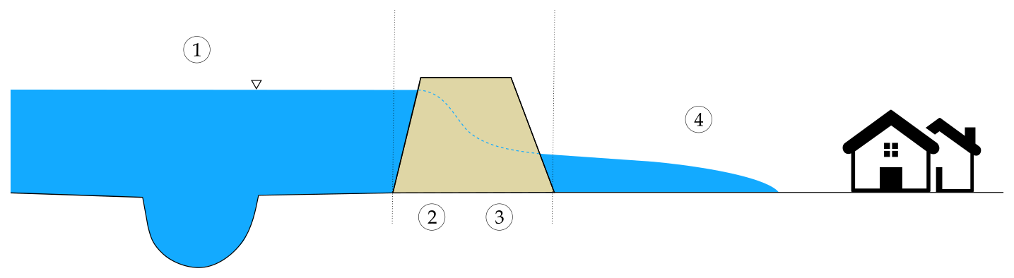
Figure 4 Schematics of a dike breach flood model, which includes (1) river flow simulation, (2) identification of failure mechanisms, (3) dike breach modelling, and (4) flood wave propagation.

The mSWE-GNN emulates only the final two-dimensional flood wave propagation. We represent all earlier-stage uncertainties by varying two key breach parameters: (i) the outflow discharge hydrograph through the breach and (ii) the breach location. The outflow is determined by the breach geometry, hydraulic boundary conditions, breach initiation, and development processes. The location depends on the geotechnical properties of the dike, which determine the dominant failure mechanism and its associated fragility curve. Instead of modelling each factor individually, we consider the hydrographs and breach locations known, and we use them as boundary conditions for the mSWE-GNN.

We generate probabilistic flood hazard maps by running ensembles of scenarios with varying boundary conditions. The outputs are aggregated into spatial probability fields, where each computational cell encodes the likelihood distribution of a flood variable (e.g., maximum water depth or flood arrival time). We summarize this uncertainty through a set of quantiles of these distributions. The reported likelihoods are conditioned on the specified boundary conditions and are therefore independent of the absolute probability of dike failure or the flood return period (that is, they are conditional on a given set of breaches and failure locations). Consequently, each scenario is assumed to occur with equal probability. To obtain unconditional occurrence probabilities, which account for the fact that different scenarios may have different likelihoods, the conditional values can be weighted by estimates of defence fragility and hydrological frequency. The integration of these defence failure probabilities and return period estimates is treated as a separate step outside the present framework and is not included in this paper.

3 Experimental setup

3.1 Case study

We selected dike ring 41, “Land van Maas en Waal”, in the Netherlands, representative of low-lying protected areas along rivers, as a case study for probabilistic flood mapping. This area is surrounded by the Meuse and Waal rivers and contains a high density of hydraulic structures. It covers 27 900 ha, supports a population of 251 900, and previous studies estimate an expected flood damage per event of EUR 5.9 billion (Rijkswaterstaat, 2016). The same study identifies piping and overtopping as the main failure mechanisms, with fragility curves that vary by dike segment. The dynamics of the flood change significantly with breach location and outflow hydrograph due to the basin slope and the presence of many elevated elements and canals (Fig. 5).

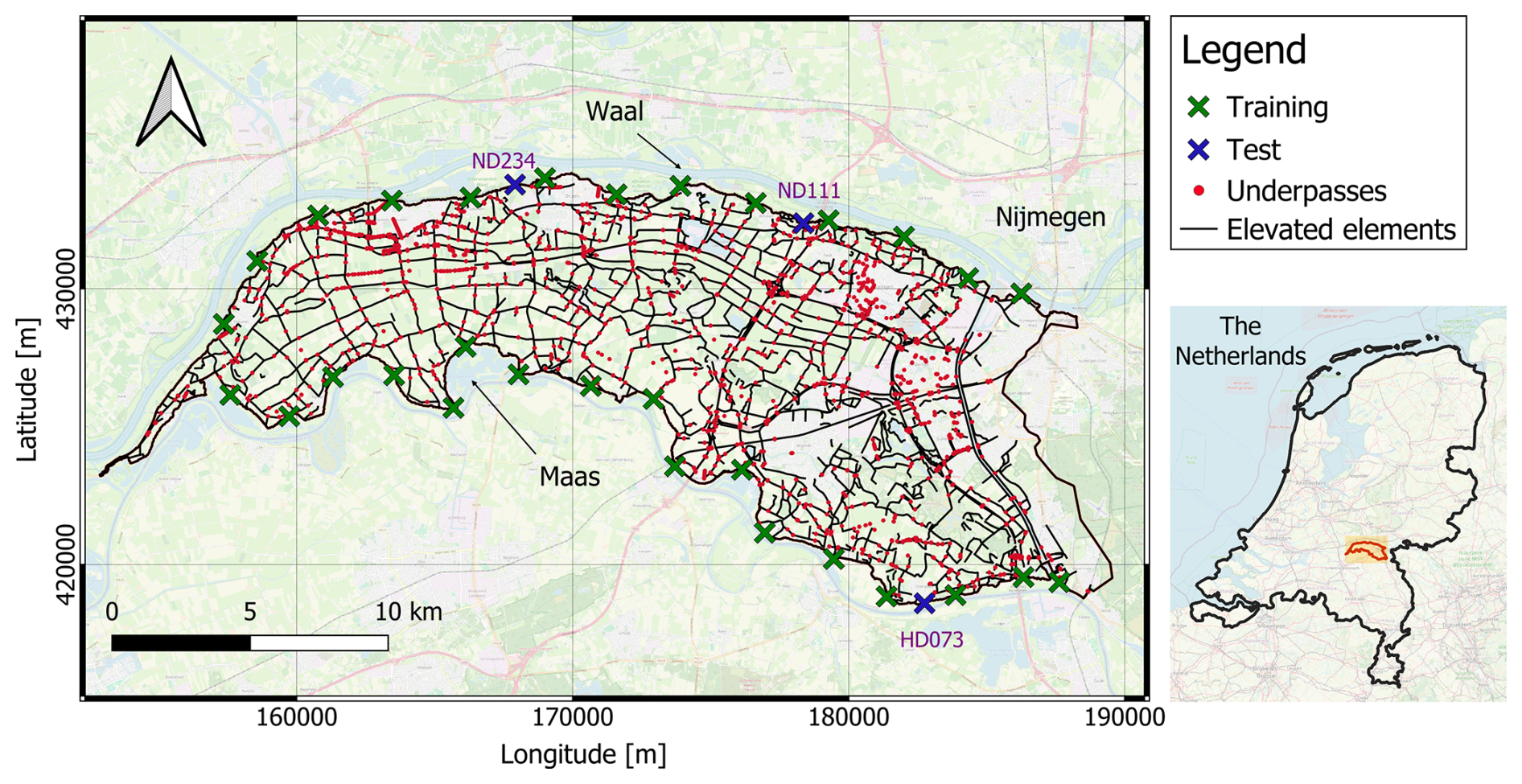
Figure 5 Dike ring 41, in the Netherlands (coordinate system EPSG:28 992 – Amersfoort/RD New). The crosses indicate the location of the dike breaches used for training and testing. The labels ND111, ND234, and HD073 indicate the three locations in the testing dataset. The maps are taken from © OpenStreetMap contributors 2025. Distributed under the Open Data Commons Open Database License (ODbL) v1.0.

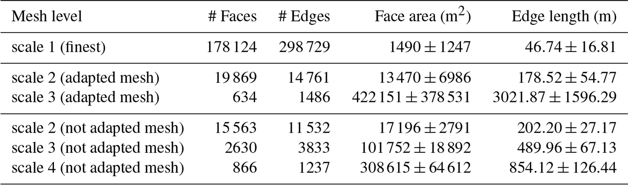
For training and validation data, we used, respectively, 30 and 10 numerical simulations performed with Delft3D (Deltares, 2022), each with a different breach location, selected to be approximately equidistant along the dike ring boundary, and a different dike outflow hydrograph over time as boundary conditions. We determined these hydrographs as in Bentivoglio et al. (2025), using synthetic hydrographs with peak discharges from 100–1500 m³ s⁻¹ (Fig. 6). All simulations use the same computational mesh, which consists of approximately 180 000 mesh faces and 300 000 mesh edges (see Table A1). For testing, we considered nine scenarios: three breach locations and three return periods of estimated river water levels (100, 1000, and 10 000 years), obtained from the Dutch national flood hazard maps (VNK) using Delft3D (Rijkswaterstaat, 2016). We selected the testing locations based on the availability of pre-computed spatio-temporal simulations and to cover a wide range of flood events, including some much larger than those in training (see Fig. 6). Each test simulation assumes instantaneous breach formation, with breach development based on the Verheij–Van der Knaap equations (Verheij and Hydraulics, 2003). Test boundary conditions are river water levels over time, determined for the Meuse and Waal rivers using the GRADE method (Hegnauer et al., 2014). Each scenario, for all datasets, uses a simulation time of 21 d and an output temporal resolution of eight hours, for a total of 64 time steps, matching the VNK simulation characteristics. All numerical simulations are run on an AMD Ryzen 7 5700X 8-Core Processor (3.40 GHz) CPU, using four OpenMP threads.

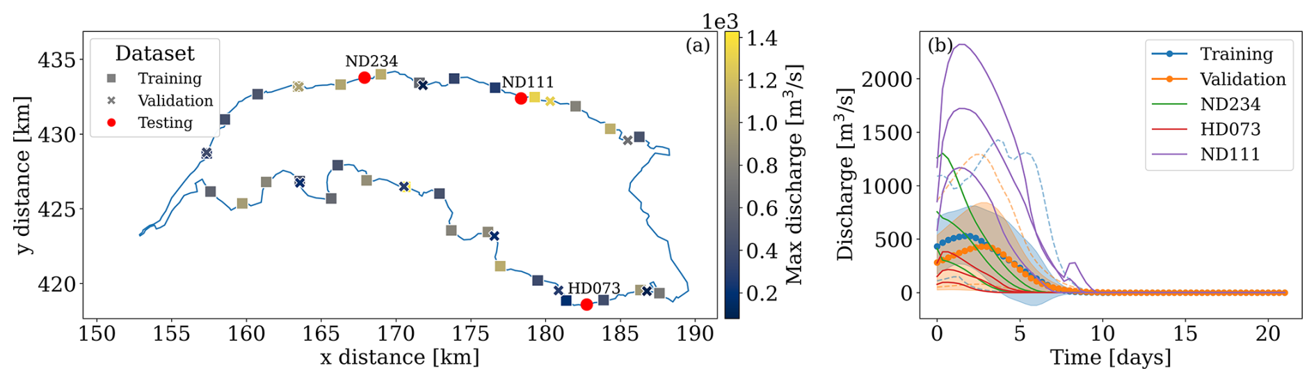
Figure 6 (a) Spatial distribution of the training, validation, and testing breach locations and associated maximum breach discharge. The north and south sides of the domain are surrounded by the Meuse and Waal rivers. (b) Training, validation, and testing discharge hydrographs used as boundary conditions for the simulations. The shaded regions indicate one standard deviation away from the mean at each time step, while the dotted lines represent the envelopes of the minimum and maximum discharges at each time step. The labels ND111, ND234, and HD073 indicate the three testing locations, with increasing discharges for increasing return period.

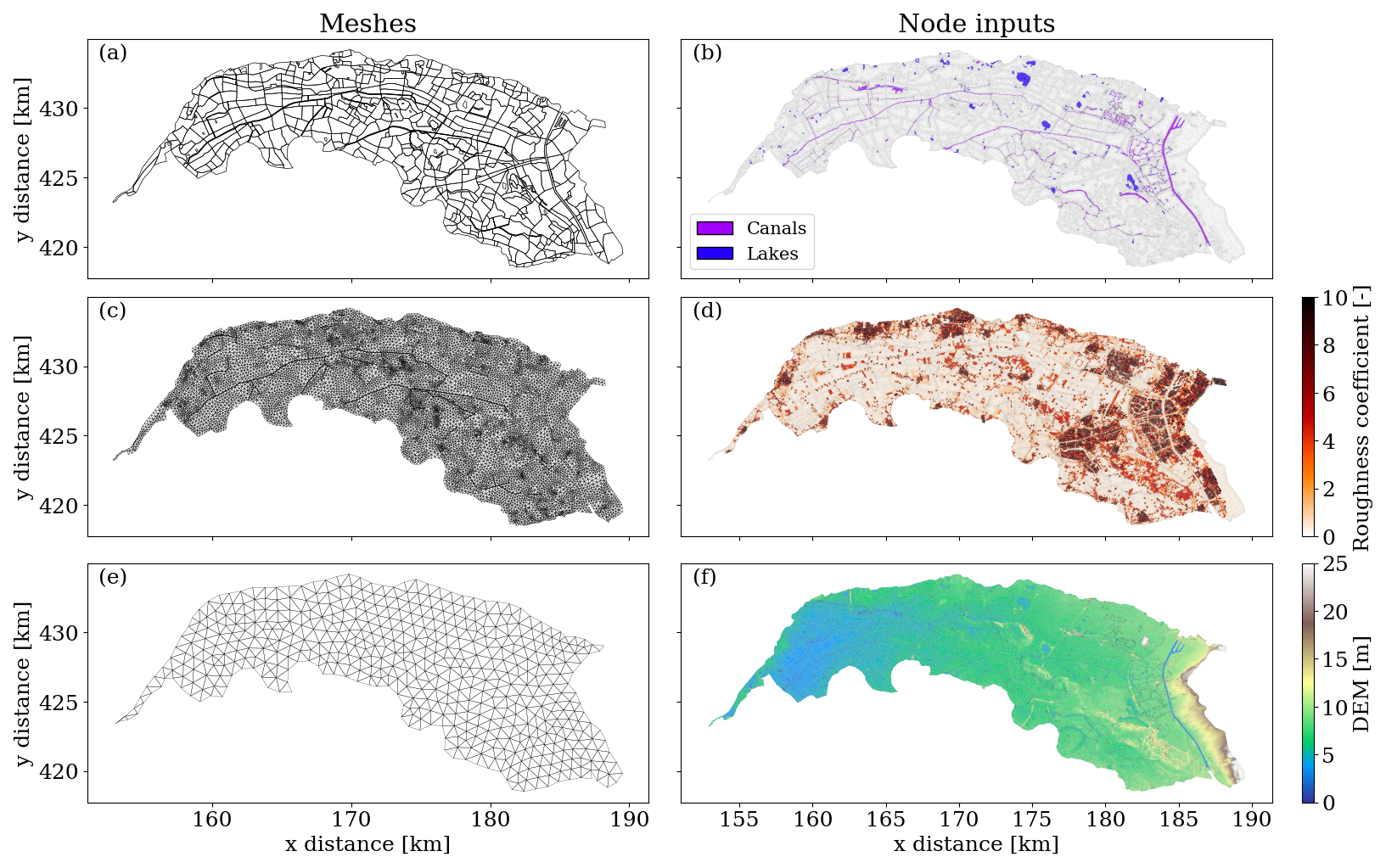
Figure 7 Part of the meshes and static node features used as inputs of dike ring 41. (a, c) represent the two coarse scales meshes (scale 3 and 2) employed in the experiments, in which the mesh polygons follow the presence of relevant hydraulic structures; (e) corresponds to an example of coarse mesh (scale 4) used in the ablation study obtained without including relevant geometrical boundaries; (b) shows the location of the canals and ponds/lakes; (d) represents the distribution of the White–Colebrook roughness coefficient, with higher values indicating urban areas; (f) shows the digital elevation model (DEM) of the area.

After training and testing, we analysed the spatial sensitivity of the model to different boundary conditions by further testing it on 100 different breach locations, each with 100 different discharge hydrographs, generated as in the training data. Each combination has the same probability of occurrence. We used this sensitivity analysis to (i) quantify the variability of the ARME under different scenarios and (ii) determine a suitable threshold for the ARME to select plausible simulations.

We then obtained probabilistic flood hazard maps of flood arrival times and maximum water depths for a given test breach location and return period. For this analysis, we used the simplified method in Besseling et al. (2025) to compute the discharge hydrographs from the river water levels. We estimated the uncertainty in breach outflow by repeatedly sampling the probability of failure of a dike segment from the dike's fragility curves for piping and overtopping, assuming different water levels over time as hydraulic loading. We performed this analysis only on test simulations, since this simplified method requires a ground-truth numerical simulation for calibration and cannot generalize to unseen locations.

3.2 Training setup

We trained all models with PyTorch (Version 2.5) (Paszke et al., 2019) and PyTorch Geometric (Version 2.6) (Fey and Lenssen, 2019), using the Adam optimizer (Kingma and Ba, 2014). Based on previous studies, we used a learning rate scheduler with a fixed step decay of 0.7 every 15 epochs, starting from 0.003. Training ran for 100 epochs with early stopping and used 16-bit mixed precision to reduce computational load. During training, we clipped gradients above two to improve stability and used a curriculum learning strategy as in Bentivoglio et al. (2023), with a maximum training prediction horizon H=5 steps ahead (Eq. 2). Although training used fixed time windows, we evaluated all validation and testing simulations over the full simulation time, without requiring any numerical solution as input. We used p=2 previous time steps as dynamic inputs, i.e., ${\mathbf{X}}_d=({\mathbf{U}}^{t-\mathrm{2}},{\mathbf{U}}^{t-\mathrm{1}},{\mathbf{U}}^t)$. The loss function coefficients (Eq. 2) were γ₁=1 for water depths and γ₂=7 for unit discharge, as in Bentivoglio et al. (2025), to give a more balanced weight to water depths, which are generally more than ten times larger than discharge values. All experiments ran on AMD INSTINCT MI200 GPUs with 64 GB RAM, provided by the LUMI cluster (EuroHPC, 2025).

We trained the mSWE-GNN with a hidden feature size of 64, three mesh scales (details found in Table A1), and a heterogeneous distribution of GNN layers across these scales. Specifically, we used two layers for the finest scale after U-Net pooling, five and three layers for the middle scale (before and after the U-Net bottleneck), and six layers for the coarsest scale. Preliminary experiments showed that adding more layers, especially before the U-Net bottleneck, increased model complexity and training time without improving performance. This is because the coarsest scale already captures large-scale flow dynamics, while the finer scales refine local details. Because of the high dimensionality of the search space and long training times (estimated at about ten hours on eight AMD INSTINCT MI200 GPUs, 64 GB), we did not conduct an extensive hyperparameter analysis.

3.3 Metrics

We measured model performance using four metrics:

• Regression. we used a multi-step-ahead mean absolute error (MAE) for each hydraulic variable ${\widehat{\mathit{u}}}_o^{\mathit{\tau }}$ over the full simulation, expressed as $\text{MAE}=\mathrm{1}/H{\sum }_{\mathit{\tau }=\mathrm{1}}^H\Vert {\widehat{\mathit{u}}}^{\mathit{\tau }}-{\mathit{u}}^{\mathit{\tau }}{\Vert }_{\mathrm{1}}$, with H being the full simulation duration.

• Classification. we used the critical success index (CSI), which measures spatial accuracy in detecting a class (e.g., flood or no-flood) for a given threshold. CSI is evaluated as $\text{CSI}=\frac{\text{TP}}{\text{TP}+\text{FP}+\text{FN}}$, where TP are true positives (cells where both numerical and deep learning models predict water depth above threshold), FP are false positives (cells where the deep learning model wrongly predicts water depth above threshold), and FN are false negatives (cells where the deep learning model does not predict water depth above threshold). We computed CSI, averaged over time, for water depth thresholds of 0.05 and 0.3 m, as in Bentivoglio et al. (2023).

• Speed-up. we measured computational speed-up as the ratio of numerical model computation time to deep learning model inference time. Both times exclude mesh creation, data pre-processing, and post-processing.

• Plausibility. we used the average relative mass error (ARME) as a validation metric to assess the plausibility of model predictions in scenarios without ground-truth simulations, as described in Sect. 2.2.

4 Results and Discussion

4.1 Model investigation

Table 1 shows the model consistently achieves high CSI values, indicating effective prediction of the spatio-temporal evolution of floods across breach locations and return periods. On the test dataset, the model attains an average CSI of 73.6 % for the 5 cm threshold and 71.1 % for the 30 cm threshold, with mean absolute errors of 64.5 cm for water depth and 1.31 m² s⁻¹ for unit discharge. The model performs best in the central range of flood volumes, where training data is concentrated, with lower errors and higher CSI values. The difference between the performance on the training and test datasets is driven by the large variability in total flood volumes, with testing volumes greatly exceeding those in training (see Fig. 6). The model also tends to over-predict flood extent for the smallest events, since the loss function penalizes larger floods more than smaller ones. Mean absolute errors in water depth tend to increase with the return period, but those for unit discharge remain relatively stable. This is because the largest values of unit discharge occur closest to the breach and then decrease over time with the inflow hydrograph, while water depths accumulate over time, leading to larger errors for more extreme floods.

Table 1 Training, validation, and testing metrics for the mSWE-GNN on dike ring 41, reporting mean and standard deviation for the mean absolute error (MAE) for water depth and unit discharge and critical success index for a water depth threshold τ (CSI_τ). These metrics are reported also for the three test locations HD073, ND234, and ND111 for the different return periods (RP). Arrows indicate whether higher (↑) or lower (↓) values are better.

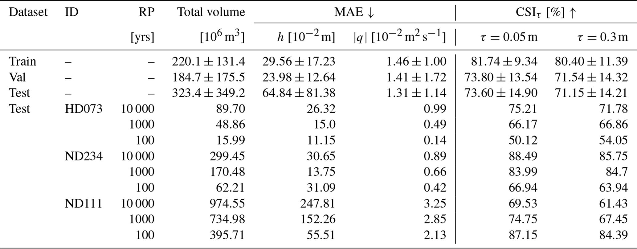
Among the three test locations, HD073 shows the lowest MAE values, due to less intense flooding. CSIs remain high except for the 100 year return period, where the breach is upstream in a sloped area and small discharge variations cause large changes in inundation. Location ND234 achieves the best overall performance, as it is located downstream and floods consistently during large events, resembling training patterns. ND111 has the highest MAEs, with all simulations producing flood volumes much greater than those in training (Fig. 6). Despite this, the model captures the spatio-temporal variability of floods, as shown by high CSI values. At ND111, all return periods nearly fill the domain with water, resulting in very high water depths, up to an average of 3.22 m covering 90 % of the domain. These results highlight that model accuracy depends on both the location and magnitude of flood events. The model performs best when test scenarios resemble training conditions, while extreme or atypical events lead to higher errors but still preserve spatial flood patterns.

4.2 Mass balance error

We tested the variability of the ARME on a set of 10 000 flood scenarios. This consisted of 100 equidistant breach locations along the breachable dike perimeter, each with 100 unique breach discharge hydrographs, generated as in training and validation. We designed this range to be purposefully much wider than for a practical scenario, to assess a more complete response of the model to different boundary conditions and locations. We define as “plausible” any simulation whose ARME is below a selected threshold.

We analysed how the ARME threshold affects the distribution of predicted flood volumes over time in Fig. 8. The number of plausible simulations increases with the threshold, as expected, with approximately 50 % of the simulations having an ARME<0.4. For higher thresholds, model predictions tend to underestimate volumes, with flood volumes capping at approximately 500 millionm³, further explaining the lower test performance for the largest floods. We can derive a similar conclusion from Fig. 9, which shows the percentage of plausible simulations for different total flood volumes and ARME thresholds. Most predictions in terms of mass conservation have a range of total volumes between 200 millions and 400 millions m³ of water. This reflects well the distribution of training simulations with a stronger bias towards higher volumes because of the training loss function that focuses more on the highest water depths.

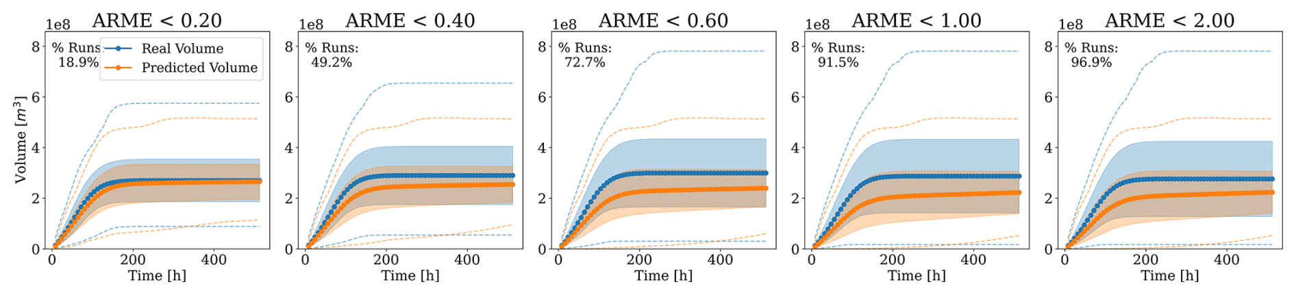
Figure 8 Comparison of real and predicted flood volumes over time for multiple ARME thresholds. The shaded regions indicate one standard deviation away from the mean, at each time step, while the dotted lines represent the envelopes of the minimum and maximum volumes at each time step. Increasing the threshold increases the number of plausible simulations but also the discrepancy, both in terms of mean and standard deviation, from the true volumes.

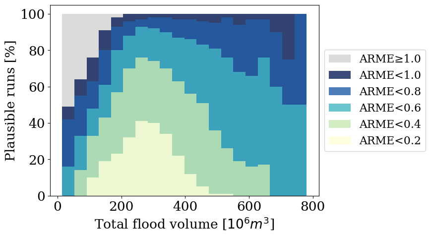
Figure 9 Percentage of plausible simulations as a function of the total flooding volume for different ARME thresholds.

Figure 10 shows how the percentage of plausible simulations changes with the ARME threshold for different breach location areas and total flood volume quantiles. Steeper curves closer to zero indicate better model performance, as more simulations have low ARME. The central volume ranges (from approximately 150–400 mil m³) yield the best performance, with most simulations having a low ARME. Figure 9 also confirms the same finding, aligning with the test dataset's optimal prediction range. Across all volume ranges, most breach locations show similar trends, meaning that the model's performance is consistent independently of the breach location. Simulations with breaches in the western downstream area (green colours) perform best across most volume ranges, with pronounced responses to ARME threshold changes, as floods starting here tend to fill the area like a bathtub, creating a recognizable flow pattern.

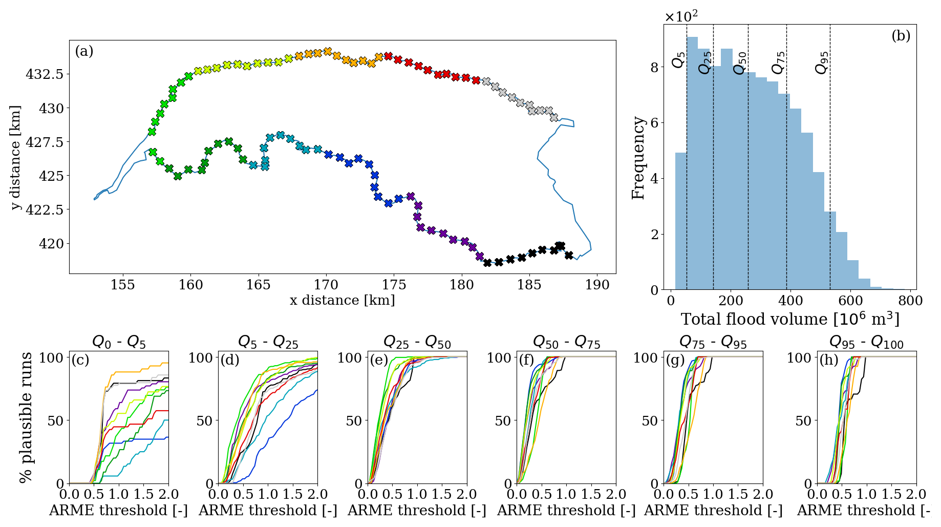
Figure 10 Percentage of plausible simulations per breach location, total flood volume ranges, and ARME thresholds. (a) Distribution of the testing breach locations. The colours represent different breach location areas, grouped by distance in 10 different zones. (b) Frequency of total flood volumes and the corresponding quantiles at 5 %, 25 %, 50 %, 75 %, and 95 %, determined from the theoretical total flood volumes in each testing simulation. (c–h) Percentage of plausible simulations for different volume quartile ranges, for increasing values of the ARME threshold.

In contrast, the highest and lowest volume quantiles, which fall outside the training range, behave worse. For the largest floods, most simulations show a sharp increase in ARME between 0.5 and 1, indicating consistent underestimation of volumes; however, even for very high discharges, the model has no instabilities, as indicated by the lack of exponentially increasing flood volume curves (Fig. 8). In the lowest volume quantiles, curves have the highest variability, as small volume errors cause larger ARME changes and lead to a bigger spread in performance. For this range, upstream locations (black, grey, and purple markers) perform better, suggesting the model understands better flow patterns for small floods when the terrain is sloped. The central-south area, dividing the western downstream bathtub region from the eastern upstream sloped one, shows more frequent errors, likely because small errors in flood routing cause larger inconsistencies, also due to the presence of several canals and elevated elements.

We evaluated the correlation between CSI and MAE with the ARME for the training, validation, and testing datasets, for which ground-truth data exists (Fig. 11). Across datasets, ARME and CSI exhibit a consistent negative dependence with correlation coefficients around −0.8, indicating that low ARME values are associated with high CSI values (Table 2). Contrarily, we found little correlation with the mean absolute errors for water depths (ρ≈0.66 only in training) and no correlation with the discharge mean absolute errors. This means that simulations with a low ARME predict well the spatio-temporal evolution of the flood and can be used as a valid proxy to determine the plausibility of testing simulations but are not always reliable in terms of hydraulic variables' values.

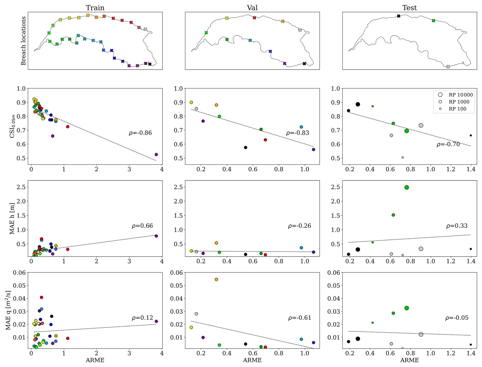
Figure 11 Distributions of ARME values for the training, validation, and testing datasets as a function of CSI at 0.05 m and MAEs for water depth (h) and unit discharges (m² s⁻¹). The colours match the location of the breach, while the size, for the testing dataset, indicates the return period.

Table 2 Pearson and Spearman correlation coefficients (with 95 % confidence intervals) between ARME and each metric across datasets. Correlations higher than 0.6 are marked in bold.

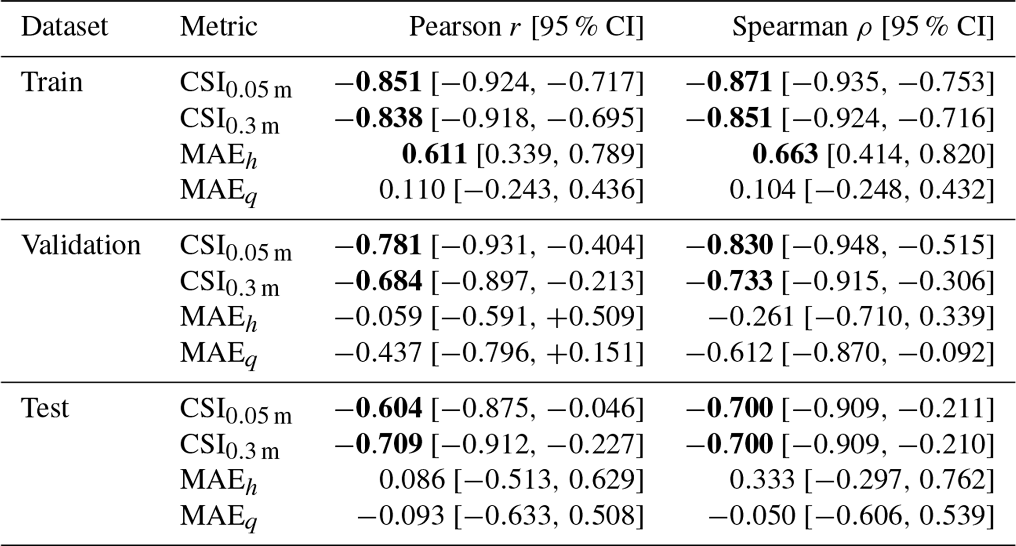
Whereas numerical models require strict mass balance with an ARME close to zero, our experiments tolerate higher variability since we do not explicitly enforce mass conservation, and an ARME<0.4 always correlates with high CSI (>0.75), which means that the spatio-temporal dynamics are well represented (Fig. 11). For this reason, we selected as a reasonable threshold an ARME=0.4, though lower values can also be employed based on the desired level of model performance. For this threshold of ARME<0.4, we analysed the spatial distribution of the percentage of plausible simulations per breach location (Fig. 12b). Similarly to what we found in the general analysis, the highest percentage of plausible simulations is associated with the western breaches, thanks to the bathtub accumulation pattern. There are also spurious locations for which no or few simulations provided had an ARME<0.4. For the two locations in the southeast border, this seems to be correlated with the presence of an area that rarely gets flooded due to the locally higher topography close to the breaches. This causes the model to severely underestimate the intensity of flooding around that area if there is a local breach and, consequently, in the rest of the domain.

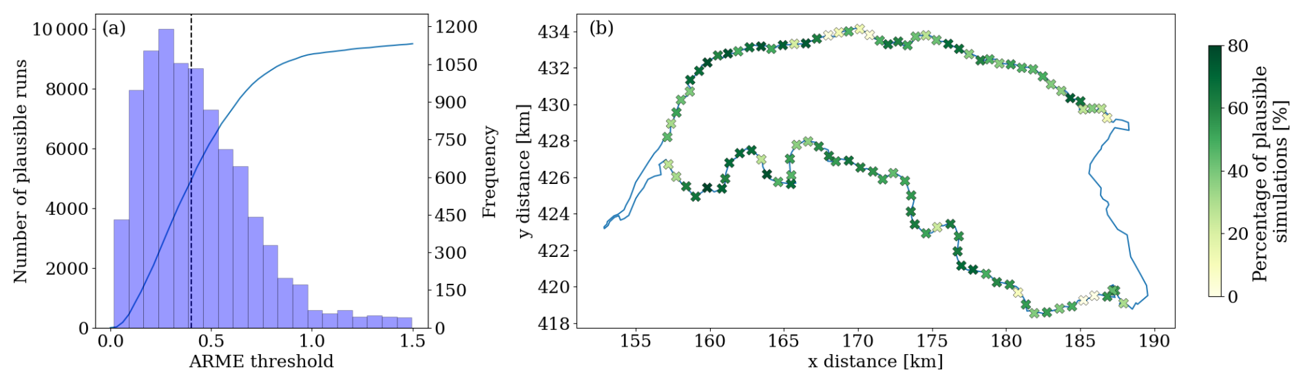
Figure 12 (a) Cumulative number of plausible simulations and frequency different ARME thresholds. (b) Spatial distribution of the percentage of plausible simulations, assuming an ARME threshold of 0.4.

4.3 Probabilistic flood mapping

4.3.1 Large-scale uncertainty

We exemplified the model in a probabilistic setting by computing the conditional probability of exceeding a certain maximum water depth for the large-scale uncertainty analysis in breach location and outflow as described in Sect. 4.2. Figure 13 shows the likelihood of having a maximum water depth higher than 0.05, 0.3, and 1 m. This probability is conditional on a breach occurring and is independent of the return period, meaning that all events have the same probability of occurrence. It is also computed over all 10 000 testing simulations with an ARME<0.4. Selecting only plausible results skews the probability distributions to be less spread out with respect to the complete set, giving a clearer distribution estimate. This analysis confirms that the western downstream area of dike ring 41 is most likely to flood due to its bathtub-like accumulation. The eastern upstream part is less likely to flood, requiring either a breach in that area or a large event.

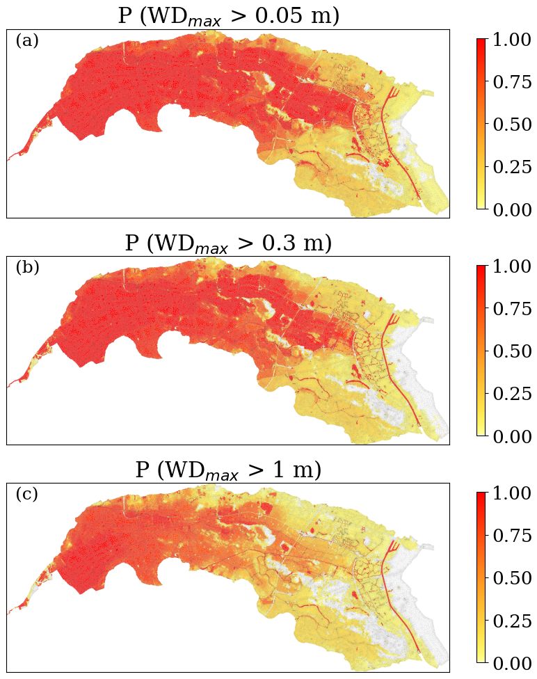
Figure 13 Predicted probabilities of maximum water depths exceeding different thresholds. They are determined using only the selected simulations among the tested 10 000 configurations that had a ARME<0.4, assuming that each simulation has the same likelihood of occurrence.

The model predicted all 10 000 simulations in about ten hours, the same average time the numerical model needs for a single numerical simulation, corresponding to a speed-up of 10 000 times. Even when considering that only 50 % of the simulations were plausible, the approach is highly efficient, highlighting its potential for large-scale probabilistic flood mapping and rapid scenario analysis.

4.3.2 Comparison of ensemble and deterministic scenarios

We quantified the uncertainty in flood hazard predictions in a test scenario by analysing the variability in maximum water depths and flood arrival times for different boundary conditions. We assumed a threshold of 0.05 m for identifying when a cell got flooded. We determined the breach outflow hydrograph from river water levels using the calibrated conceptual method in Besseling et al. (2025). This approach models breach evolution and outflow as either free flow or submerged flow, depending on whether the breach is unconfined or confined. The outflow is calibrated via a parameter fitted using a ground-truth reference outflow from a numerical simulation. The outflow hydrographs served as boundary conditions for the trained mSWE-GNN model. We compared the ensemble results against the single-scenario prediction and its corresponding ground-truth simulation. We refer to this single prediction as the “deterministic” result.

We selected breach location HD073 and a return period of 10 000 years as a representative test. Using only non-identical hydrographs, sampled from the fragility curves, we obtained 206 different boundary conditions. Considering only simulations with ARME below 0.4, 25 % of the ensemble produced flood volumes over time close to the ground truth (Fig. 14). While the deterministic prediction tends to overestimate the final flood volumes, plausible ensemble members provide a more accurate representation of the flood dynamics, both in terms of maximum water depths (Fig. 15) and flood arrival times (Fig. 16). The 50th percentile of the ensemble predicts lower water depths and slower propagation compared to the deterministic case, aligning more closely with ground-truth observations. Although these predictions do not exactly correspond to the ground-truth simulation, as they assume a smaller outflow discharge, they demonstrate that the model's performance can improve with slight adjustments to boundary conditions when selecting simulations with smaller ARME.

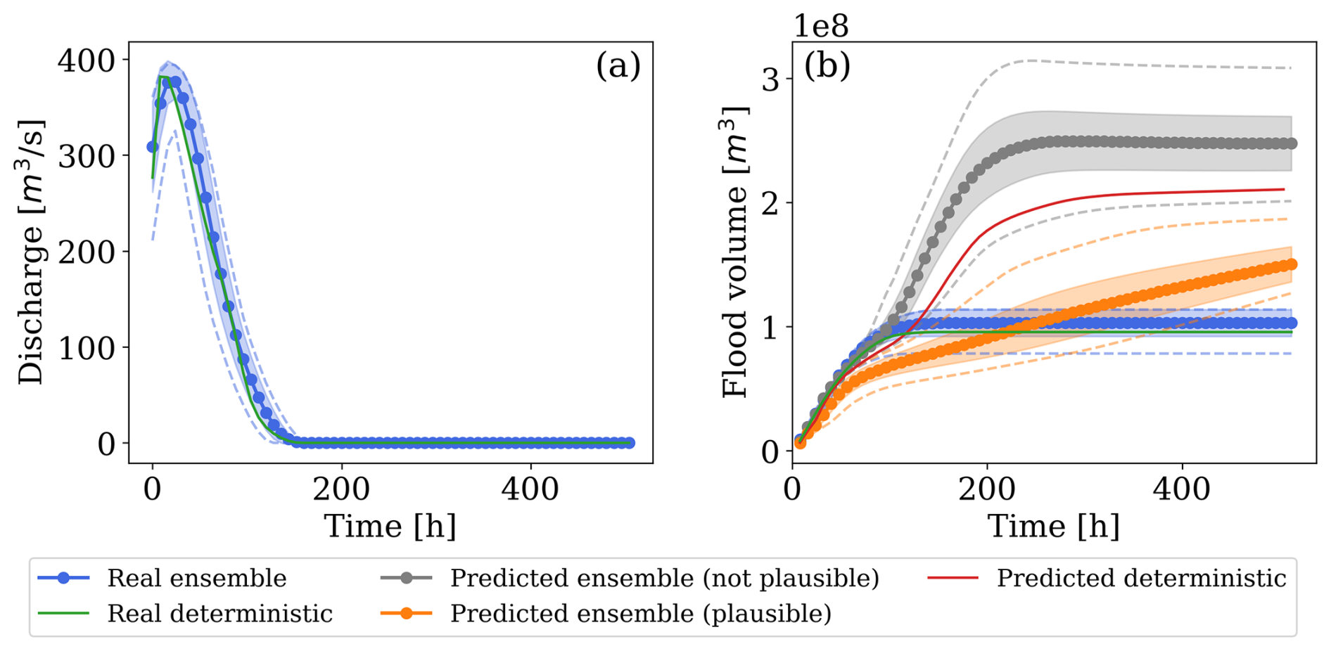
Figure 14 Range of discharges and volumes over time for the deterministic and ensemble cases, for true values and predicted ones, plausible and not. The shaded regions indicate one standard deviation away from the mean at each time step, while the dotted lines represent the envelopes of the minimum and maximum volumes at each time step.

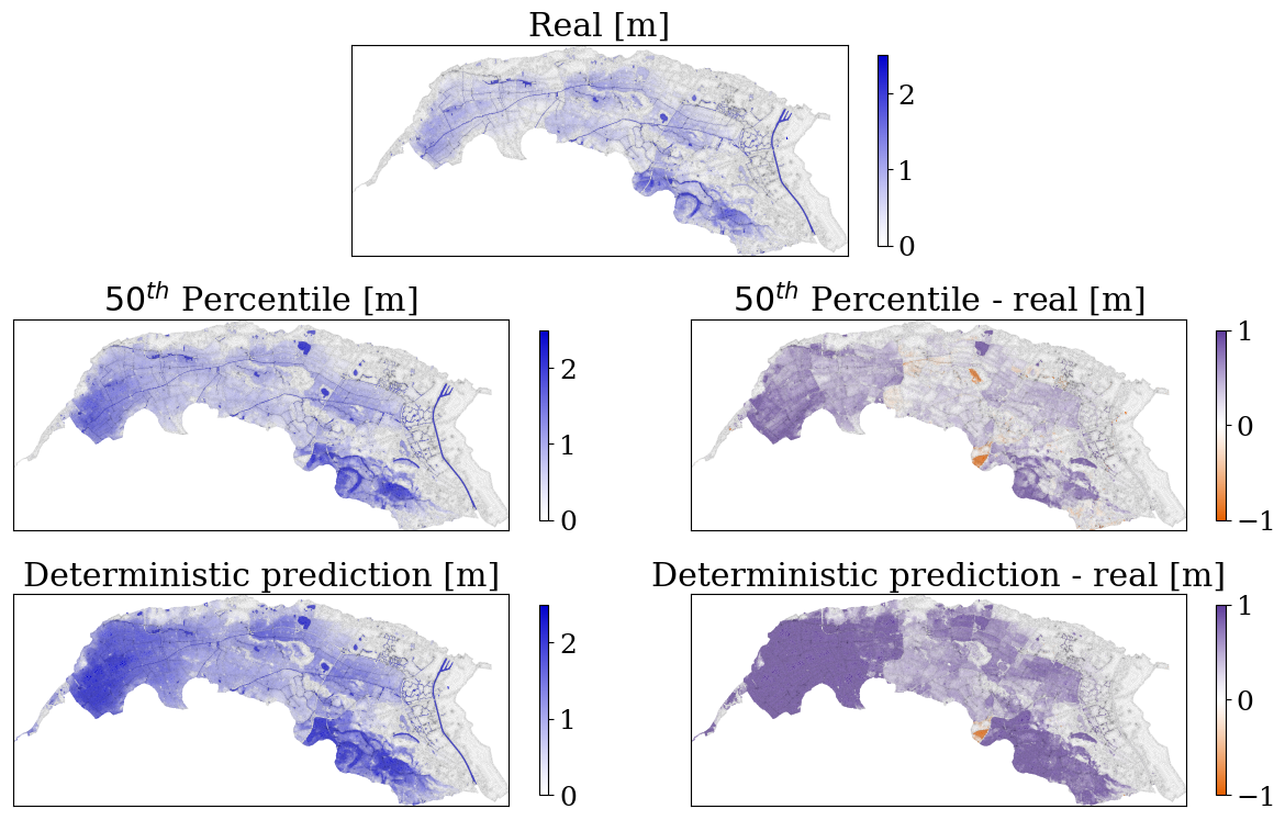
Figure 15 mSWE-GNN ensemble predictions of maximum water depths [m] for the 50th percentile compared to the ground-truth numerical simulation for breach HD073 and a return period of 10 000 years. The plots on the right side represent the difference between the mSWE-GNN predictions and the numerical model's.

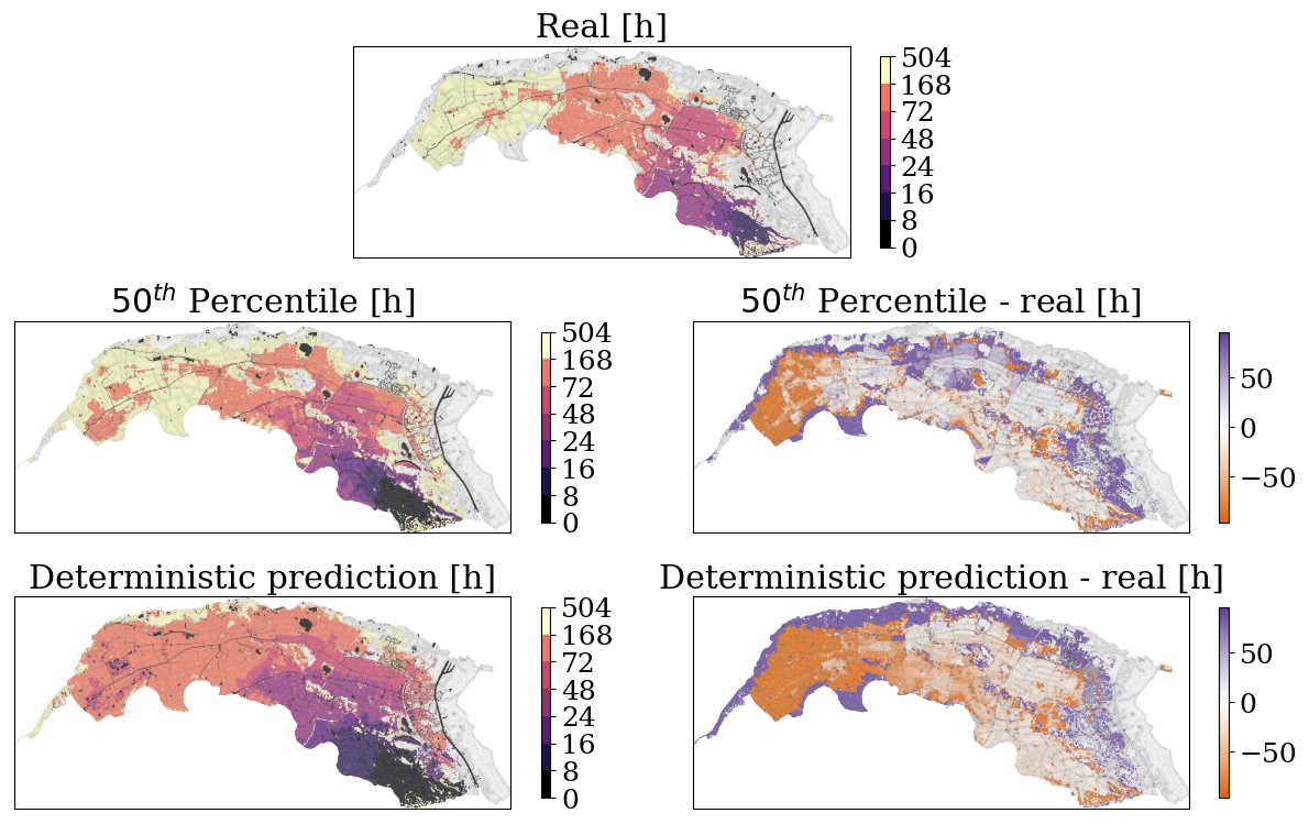
Figure 16 mSWE-GNN ensemble predictions of flood arrival times (h) for the 50th percentile compared to the ground-truth numerical simulation for breach HD073 and a return period of 10 000 years. The plots on the right side represent the difference between the mSWE-GNN predictions and the numerical model's.

The predicted spread of the ensemble is larger than the theoretical one calculated from the boundary conditions (Fig. 14b), primarily because the chosen location is upstream of multiple hydraulic structures, making it especially sensitive to minor variations in outflow discharges, as also reflected in the elevated training error for one of the upstream breaches (Fig. 11, purple marker). This sensitivity is also amplified by the limited amount of training data, which makes the model's response more variable in these conditions. In contrast, predicted uncertainty is lower for smaller events and downstream locations, where the influence of small variations in boundary conditions is reduced, leading to more stable and consistent predictions.

4.4 Ablation study: including hydraulic structures

We analysed the impact of hydraulic structures as node and edge features and coarse mesh, as discussed in Sect. 2.1.2. For the case without adapted coarse meshes, we used four scales (details found in Table A1) instead of three to compensate for the lack of elongated cells. As in the base architectures, we distributed GNN layers heterogeneously across scales: two layers for the finest scale after U-Net pooling, three and four layers for scale one (before and after the U-Net bottleneck), four and two layers for the coarser scale, and six layers for the coarsest scale.

Table 3 shows that all proposed changes improved most metrics (row 1, base model). Using coarse meshes that fit existing hydraulic structures produced the largest improvement (cfr. row 5, w/o adapted coarse meshes), likely due to better treatment of canals, which convey water quickly in a specific direction. In GNN models, the number of layers should match the speed of water propagation within a given time range, set by the model's time step. Adding longitudinal mesh elements allows water to move efficiently without requiring many GNN layers. However, adapting the meshes alone, without including edge features for hydraulic structures, led to worse results, especially in testing (row 4, only adapted coarse meshes). This suggests that while mesh adaptation helps, it is insufficient alone; the model also needs explicit information about hydraulic structures to learn their effects on flood propagation.

Table 3 Ablation study for the inclusion of hydraulic structures in the model as node, edge, or mesh features. w/o = without. The best results for each metric and for each dataset are highlighted in bold.

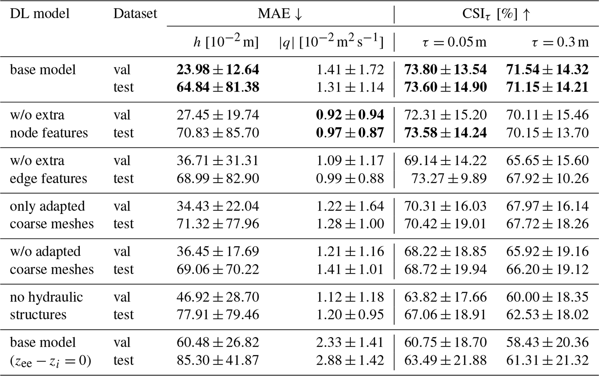
Adding elevated elements as an edge feature improved results mainly in validation (cfr. row 3, w/o extra edge features). Its effect on the test dataset was less pronounced, likely because very large floods overtop elevated elements easily. To further validate the importance of elevated elements as edge features, we also tested the base model after setting these values to zero (row 7, base model $z_{\text{ee}}-z_i=\mathrm{0}$). The marked drop in performance confirms that the model has effectively learned to account for the influence of these structures on flow dynamics.

Marking lakes and canals with a binary node feature had the least impact (row 2, w/o extra node features), probably because the model already learns this information from the water variable vectors. However, removing these features improved the MAE for unit discharge for both validation and testing datasets. This suggests that the model can infer the presence of these structures from the flow patterns, and explicitly providing this information may not be necessary.

5 Conclusions

This study demonstrated the feasibility of using deep learning surrogates for probabilistic flood hazard mapping in real case studies. To this end, we included hydraulic structures such as canals, underpasses, and elevated roads as model inputs and introduced the average relative mass error (ARME) as a physically-based plausibility metric to validate the model in the absence of ground-truth data. With this framework, we generated probabilistic flood maps that quantify uncertainty in maximum water depths and flood arrival times for varying breach locations and discharge hydrographs.

We found a strong correlation between the ARME and the critical success index (CSI), confirming the ARME's value as an indicator of simulation reliability when reference data are unavailable. In a large-scale analysis of 10 000 scenarios, approximately half of them produced physically consistent outcomes, predominantly within mid-range breach outflows, suggesting that model generalization remains most reliable within trained discharge regimes. Beyond quantifying uncertainty, the framework offers a practical tool for identifying locations most sensitive to input variations and for prioritizing expensive numerical simulations, thereby improving the efficiency of flood risk assessment.

While the current study focused on a single case study and simplified breach representation, future research should validate the framework for multiple interacting breaches, integrate dynamic river and breach evolution models, and validate across diverse case studies. Moreover, future studies could include other sources of uncertainties, such as river water levels or floodplain roughness (Hall and Solomatine, 2008). Future studies should also include the probabilities of dike failure by comparing the expected hydraulic loads and the geotechnical properties of dike segments to obtain a complete probabilistic map (e.g., Jongejan and Maaskant, 2015). Moreover, future works could explore the use of mixture-of-experts models to improve the model performance across a wider range of boundary conditions, for example, by combining or selecting the output of different models, each trained with a smaller range of conditions.

Overall, this framework advances the deployment of rapid surrogate models for probabilistic flood analysis and flood hazard mapping. It enables real-time scenario assessment, quantifies flood variability for different locations and boundary conditions, and helps identify the most critical breach and discharge combinations. These capabilities support more effective and efficient flood risk management and represent a significant step toward operationalizing deep learning surrogates in flood risk assessment.

Appendix A: Mesh details

Table A1 Summary of mesh characteristics for the different meshes used in the mSWE-GNN, for both the baseline case with meshes adapted to hydraulics structures and without adaptation (Sect. 4.4).

Appendix B: List of Acronyms

CSI	Critical Success Index
DL	Deep Learning
GNN	Graph Neural Network
mSWE-GNN	Multi-scale Shallow-Water-Equations Graph Neural Network
GPU	Graphical Processing Unit
ARME	Average Relative Mass Error
VNK	Veiligheid Nederland in Kaart (Dutch national flood hazard maps)