Pan-European assessment of coastal flood hazards

Coastal flooding is among the most damaging natural hazards in Europe, yet large-scale assessments have typically relied on simplified static “bathtub” models and coarse elevation data. Here, we present a novel pan-European methodology that applies a dynamic flood model at 25 m resolution, forced by location-specific total water level hydrographs. These hydrographs integrate mean sea level, tides, storm surge, and wave setup with spatially varying foreshore slopes, allowing storm type, duration, and shape to be explicitly represented. More than 51 000 coastal target points were used to reconstruct events, and the methodology was validated against 12 local-scale historical floods across diverse coastlines. The validation results confirmed the robustness of the large-scale methodology while highlighting the strong dependence of the results on the resolution and vertical accuracy of the underlying digital elevation model. At continental-scale, sensitivity analyses quantified uncertainty from model selection, hydrograph shape, and storm type. Results show that static flood models systematically overestimate inundation, with errors exceeding 25 % in low-lying coastal floodplains such as Belgium and the United Kingdom. At the continental scale, storm type variability explains 41 % of flood map uncertainty, while hydrograph shape has a smaller but measurable effect. Including coastal protection standards reduces the estimated exposed floodplain by more than half, underscoring the critical role of defenses. By bridging the gap between global static assessments and local dynamic models, this study establishes a methodological benchmark for continental-scale flood hazard mapping.

1 Introduction

Coastal flooding caused by extreme events poses a major threat to communities, assets, and critical infrastructure located in exposed coastal zones. Historic examples, such as the 1953 North Sea flood, which affected more than 750 000 people in the Netherlands, the United Kingdom, and Belgium (Gerritsen, 2005), highlight the devastating consequences of such events. More recent storms, including Hurricane Katrina in 2005 (Knabb et al., 2023), Xynthia in 2010 (Rouhaud and Vanderlinden, 2022), Babet in 2023 (Kiesel et al., 2024a), and Ciarán in 2023 (Reuters, 2023), caused billions of euros in damages, widespread disruption, and significant loss of life. These events demonstrate that coastal flooding continues to impose severe economic and societal costs with impacts and consequences ranging in nature and magnitude.

Assessing coastal flood impacts is essential for informed decision-making, as it provides critical information on potential consequences and supports timely and effective disaster preparedness. Large-scale assessments are particularly valuable because they help identify hotspots where detailed local analyses are needed before resources are allocated to risk reduction measures. These studies typically combine hazard and exposure data through impact modeling to generate flood maps, which can then be intersected with population, asset, and vulnerability information to estimate risk. While some methodologies exist at the continental or global scale (Li et al., 2025; Wing et al., 2024), there remains a need to improve the generation of flood maps themselves, as they form the foundation of these frameworks.

In large-scale impact assessments, climate hazards are commonly represented by the total water level (TWL), which combines wave conditions, storm surge, astronomical tide, and mean sea level. Flooding occurs when extreme TWL exceeds local thresholds such as natural topographic barriers or coastal protection infrastructures (van de Wal et al., 2024), inundating low-lying coastal areas typically represented by digital elevation models (DEMs). Four key challenges constrain the accuracy of large-scale flood studies: (1) the choice of the flood modeling approach, which strongly influences other methodological decisions; (2) the characterization of marine boundary conditions related to TWL, including foreshore slope, wave setup, and storm hydrographs; (3) the spatial resolution and coherence of both boundary conditions and terrain data; and (4) validation of the methodology to ensure robustness.

Flood modeling approaches range from static, GIS-based “bathtub” methods to dynamic, process-based models that simulate flood propagation using shallow-water equations. Static models are computationally efficient and widely used at global (Hallegatte et al., 2013; Hinkel et al., 2014; Muis et al., 2016; Kirezci et al., 2020) and continental scales (including Australia (O'Grady et al., 2024), West Africa (Dada et al., 2023), the United States (Climate Central, 2025), and Europe (Mokrech et al., 2015; Forzieri et al., 2016; Groenemeijer et al., 2016; Paprotny et al., 2018)). However, they neglect bottom friction, dynamic sea level components, and floodwater spreading. This often leads to systematic overestimation of flood extents. Dynamic flood models, such as LISFLOOD-FP (Bates and De Roo, 2000), RFSM-EDA (Jamieson et al., 2012), and SFINCS (Leijnse et al., 2021), overcome these limitations by explicitly simulating flood propagation, but they are computationally demanding and require high-quality input data and validation. As a result, only a handful of studies have applied dynamic modeling to global (Wing et al., 2024), continental (Vousdoukas et al., 2016, 2020; Le Gal et al., 2023), and regional scales (Kiesel et al., 2023; Leijnse et al., 2025).

Marine boundary conditions refer to the definition of the TWL, which is typically represented as the sum of tide, surge, and waves (Pugh, 1987). Yet, large-scale studies often omit or oversimplify some of these components, particularly regarding the wave contribution which is frequently neglected (Muis et al., 2016; Paprotny et al., 2018). When included, the wave contribution to TWL is commonly represented as wave setup, i.e., a quasi-steady (time-averaged) elevation of the mean coastal water surface at the shoreline induced by wave breaking. Wave setup should be distinguished from wave runup, which describes the oscillatory vertical excursion of the shoreline driven by swash motions and typically includes both infragravity and incident components (Stockdon et al., 2006). In this study, we represent the wave contribution via setup rather than runup because the large-scale estimation of infragravity swash remains highly uncertain and would introduce poorly constrained spatial variability. In addition, the incident swash component primarily manifests as intermittent uprush (“splashing”) at the shoreline; while it can contribute to localized overtopping, it typically does not translate into sustained water-level elevations or flood volumes that generate persistent inundation footprints and damages at the spatial and temporal scales targeted here. The most widely used formulation of wave setup is the empirical approach of Guza and Thornton (1981), which estimates wave setup as 20 % of the significant wave height (Hs). However, this method often overestimates setup (Hinkel et al., 2021). More accurate alternatives involve simplified parameterizations, such as the semi-empirical formulation by Stockdon et al. (2006). In addition to wave information, parameterizations such as these require estimates of foreshore slope, which represents another key challenge for large-scale studies. To address this challenge, some authors have adopted a constant slope of 1 : 30 (Kirezci et al., 2020), while others have applied formulations designed for dissipative beaches that do not require slope data (Stockdon et al., 2006; Vitousek et al., 2017). An alternative approach developed by Sunamura (1984) allows estimation of spatially and temporally varying foreshore slopes from wave conditions. Compared with locally observed slopes or globally constant values, this method accounts for morphological feedback, as evolving beach morphology can influence wave contributions to sea level (Melet et al., 2020). Beyond these challenges, which are common to both static and dynamic flood models, dynamic models face an additional requirement: information on the temporal evolution of storms through hydrographs. Defining TWL hydrographs, including storm duration and shape, has rarely been attempted in large-scale studies, despite clear evidence that these factors strongly influence flood extent (Höffken et al., 2020).

Data resolution represents the third major limitation. The resolution of DEMs largely determines the quality of flood maps, with finer DEMs generally improving the representation of terrain features such as coastal defenses, channels, and drainage pathways. Until recently, the highest-resolution global-scale flood assessments used 1 km DEMs (Muis et al., 2016; Kirezci et al., 2020), while the finest continental-scale application reached 100 m resolution (Groenemeijer et al., 2016), both relying on static flood models. Applications of dynamic flood models at large scales remain limited, though new advances have produced flood maps at 30 m globally (Wing et al., 2024) and 90 m across Europe (Vousdoukas et al., 2016). As remote sensing and lidar-derived topography data continue to improve, high-resolution DEMs such as EU-DEM (Copernicus, 2019a), FABDEM (Hawker et al., 2022), and DeltaDTM (Pronk et al., 2024) allow for more accurate flood maps to be produced. For process-based flood maps, the quality and resolution of land-use information further influence the results, as land cover strongly affects overland hydraulic flow and flood propagation. The most widely used dataset for this purpose is CORINE Land Cover at 100 m spatial resolution (EEA, 2018), which is typically converted into terrain roughness values.

In addition, the resolution of marine forcing data (tides, surges, and waves) is often much coarser, creating inconsistencies with terrain datasets. When neglecting the wave contribution, these inputs are available at 2.5 km resolution globally and 1.25 km in Europe (Muis et al., 2020). When including the wave contribution, studies have achieved ∼ 70 km resolution globally (Kirezci et al., 2020) and at continental-scale up to 2.5 km resolution (Le Gal et al., 2023). Balancing resolution against computational feasibility therefore remains a central challenge for continental-scale flood hazard modeling, mainly because spatially consistent data at high enough resolution is often not available.

Finally, to balance accuracy with feasibility, large-scale coastal flood impact assessments often rely on assumptions and simplifications. Validating these choices is therefore essential, even when high-quality data and reliable models are used. While the validation of boundary conditions has been widely explored (e.g., Dalinghaus et al., 2025; Kirezci et al., 2020; Treu et al., 2024; Vousdoukas et al., 2018), the validation of the flood extent remains a challenge at the large scale due to the scarcity of observational records. This limitation is critical because flood extent is the primary output used to quantify exposure and damages, and thus underpins risk estimates. Comprehensive inundation-footprint validation is therefore essential, yet it is still rarely undertaken beyond local case studies. Here, this gap is addressed with the objective of strengthening the confidence in the risk-relevant outputs. In addition to the validation, it is equally important to understand the reason behind its results as they can indicate potential sources of uncertainty or opportunities for methodological improvement. A common approach is to reproduce specific historical flood events at the local scale (Paprotny et al., 2018; Vousdoukas et al., 2016). Ideally, the set of validation cases should encompass a range of storm types and coastline settings and be spatially distributed across the study area (Le Gal et al., 2023). Although systematic global-scale flood-extent validation has recently been demonstrated for riverine flooding (Sadana et al., 2025), to the best of our knowledge, comparable large-scale coastal flood methodologies have rarely been validated in a systematic manner against high-resolution, local-scale inundation observations across multiple historical events and diverse coastal settings, including the analyses needed to benchmark alternative input datasets and methodological choices (Table S1 in the Supplement). As a consequence, validation is an underdeveloped step in large-scale flood modeling despite its essential role. Without robust validation, the reliability of large-scale flood projections remains uncertain.

This study addresses these challenges by developing and applying a methodology for continental-scale coastal flood hazard assessment, with Europe as a pilot case. The approach combines a 25 m resolution DEM with 30 m land-use that is used to generate flexible topographic meshes and more than 51 000 location-specific TWL hydrographs that incorporate peak water level, storm duration, storm shape, and spatially varying foreshore slopes. These meshes and hydrographs are then used as inputs to the dynamic flood model RFSM-EDA to simulate process-based flood propagation across the European coastline. The methodology is validated against 12 historical flood events spanning diverse storm types and coastal settings. Although similar large-scale coastal flood modeling approaches have been presented and validated for Europe (e.g., Le Gal et al., 2023; Vousdoukas et al., 2016), though with lower resolutions and different input data, the present study is supported by a series of sensitivity analyses used to quantify the influence of key assumptions within the modeling chain. For instance, the methodology is further tested through sensitivity analyses of model choice, hydrograph shape, storm type variability, and coastal defenses. By quantifying the relative contribution of these uncertainty sources, the study establishes a methodological benchmark for large-scale coastal flood assessments. Beyond advancing scientific understanding of extreme coastal flooding processes, the framework also provides a basis for identifying hazard hotspots and informing adaptation planning and risk management at the European scale.

2 Datasets

2.1 Marine forcing input

Hydrographs of extreme total water level (TWL) events were generated for the entire European coastline to serve as marine forcing in the flood model. In total, 51 010 coastal target points (CTPs) were defined at 1 km intervals along the shoreline. CTPs were located at a relative depth of 0.1 ($h/L$; where h represents the water depth and L the corresponding wavelength of the wave peak period with an exceedance probability of 0.1). For each CTP, hydrographs were constructed by combining three elements: (i) peaks obtained from extreme value analysis, (ii) event durations determined from a storm classification and duration functions, and (iii) shapes based on the mean storm conditions at the given location.

In this study, TWL is considered as the main indicator of extreme sea level, defined as the linear sum of mean sea level, astronomical tide, storm surge, and a wave setup component. Local mean sea level was used as the benchmark. Astronomical tide hourly time series were reconstructed from tidal constituents of the TPXO9 model (Egbert and Erofeeva, 2002) with a coastal resolution of $\mathrm{1}/\mathrm{30}$° (∼ 3.5 km). Storm surge time series were derived from a European regional hindcast using the ROMS model (Shchepetkin and McWilliams, 2005) at 5–11 km resolution. The wave component was obtained from a downscaled swell hindcast generated with WaveWatch III (Tolman, 2009) at $\mathrm{1}/\mathrm{8}$° (∼ 10–15 km). Downscaling followed the DOW approach (Camus et al., 2013), combining numerical simulations with SWAN (Booij et al., 1999) and statistical methods to achieve 1 km resolution along the European coastline. Both the storm surge and wave datasets were forced with ERA5 reanalysis wind and pressure fields (Hersbach et al., 2020) and produced by IHCantabria (2024a). The wave dataset also accounts for ice cover as a limiting factor for wave generation.

Wave setup was calculated using the semi-empirical formulation of Stockdon et al. (2006), with spatially variable intertidal slopes derived from Sunamura (1984). The complete TWL time series was reconstructed for 1985–2021 on an hourly basis at each CTP.

2.2 Terrain and land use

Digital elevation models (DEMs) were used to build the computational meshes of the flood model, covering the entire coastal region of Europe, including the IPCC continental Europe region as well as the Spanish territories of the Canary Islands, Ceuta, and Melilla. The baseline dataset was the Copernicus EU-DEM at 25 m resolution with the associated EEA coastline (Copernicus, 2019a; EEA, 2017). Since the EU-DEM does not cover parts of Russia, the Canary Islands, Ceuta, and Melilla, additional DEMs were merged into a single homogeneous dataset. For Russia, the Copernicus EU-DEM at 30 m (Copernicus, 2019a) was used, while for the Spanish territories the 5 m DEM of the National Geographic Institute was adopted (IGN, 2019). The final study area (floodplain) was defined as zones between 0 and 15 m elevation with a hydraulic connection to the sea.

Because process-based flood models are sensitive to terrain roughness, spatially variable roughness coefficients were inferred from the 30 m ODSE-LULC land cover dataset (Witjes et al., 2022). In areas not covered by ODSE-LULC, such as Russia and western Turkey, the 100 m Global Land Cover dataset (Copernicus, 2019b) was used instead.

3 Methodology

To apply a process-based flood model at continental scale, we developed a three-step methodology (Fig. 1):

1. Preparation of marine boundary conditions with spatially variable, location-specific TWL hydrographs for extreme events of different return periods, including distinct peak water levels, storm durations, and hydrograph shapes.

2. Generation of flexible and irregular topographic meshes for the flood model, incorporating terrain roughness inferred from land-use information.

3. Hydraulic simulations with the process-based flood model RFSM-EDA to produce flood maps for a range of extreme scenarios.

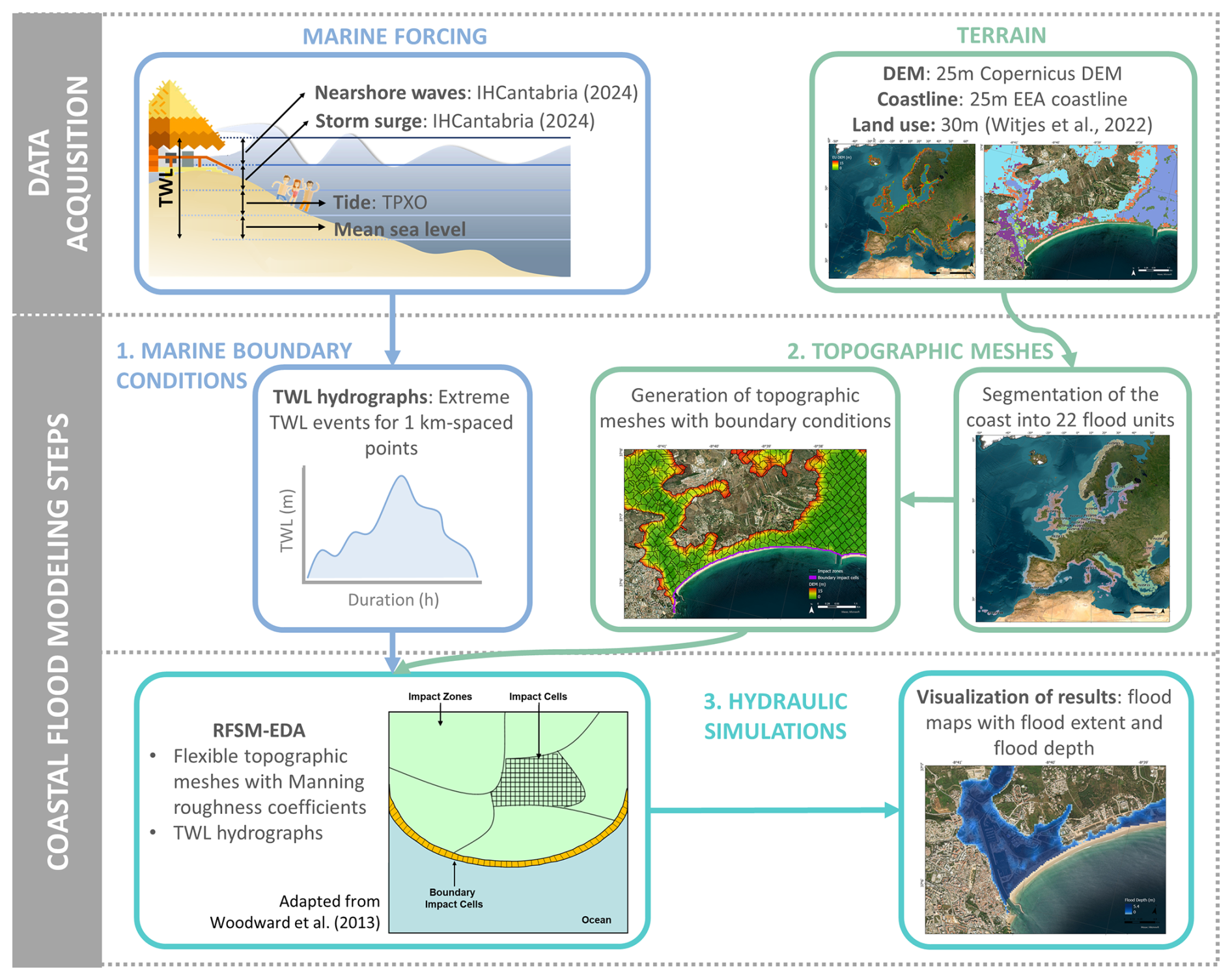
Figure 1 Continental-scale coastal flood modeling methodology applied. The methodology is divided into data acquisition and coastal flood modeling with its three steps: (1) preparation of marine boundary conditions; (2) generation of topographic meshes; and (3) hydraulic simulations. The top-left and center-left panels were created by the authors. The bottom-left panel is modified from Woodward et al. (2013, their Fig. 1). Background satellite imagery credits: Maxar, Microsoft, and Earthstar Geographics.

3.1 Preparation of marine boundary conditions

Following Cotrim et al. (2025a), marine boundary conditions were represented by TWL hydrographs constructed for each CTP and composed of three elements: peak, duration, and shape.

Table 1 Brief description of the storm types analyzed at the continental-scale coastal flooding simulations.

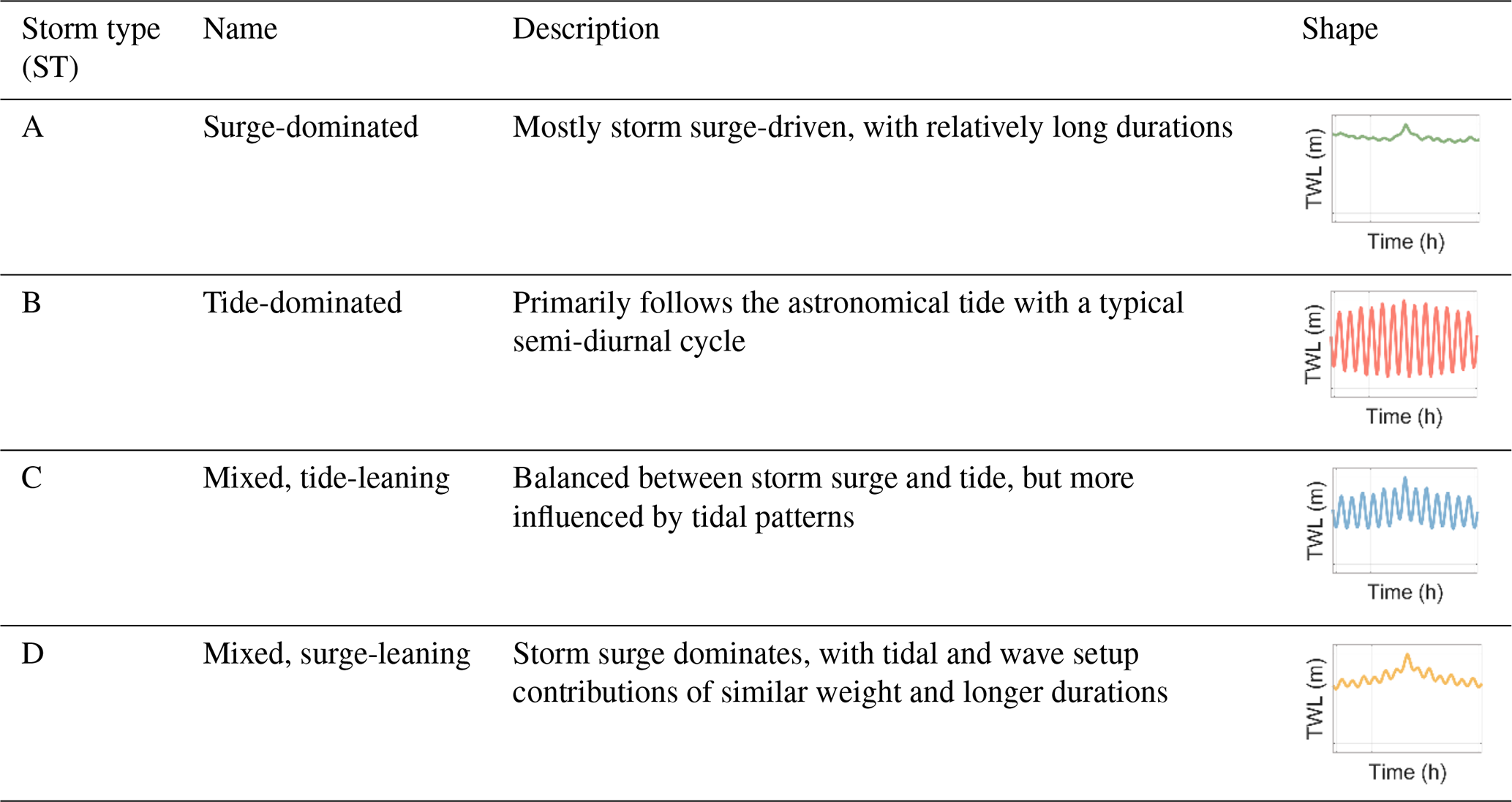
Peak water levels were estimated through extreme value analysis (EVA), using an exponential model fitted to extreme events identified in the 37-year TWL hindcast. Events were selected using the peak-over-threshold (POT) method, with a spatially variable threshold yielding on average two events per year and requiring a minimum 72 h interval between events. Sensitivity analyses on the POT threshold and distribution fits indicated the EVA method selected to provide the most appropriate balance of accuracy, robustness, and sample size. For more details on the TWL reconstruction method and the EVA, please refer to Cotrim et al. (2025a). Hydrograph duration was derived from a storm duration function calibrated with historic storms (i.e., all events identified by POT) that combined a storm type (ST) classification with individual storm duration estimates. The storm classification system was based on hydrograph shape through Manhattan Dynamic Time Warping and reflected the dominant TWL drivers at peak conditions. Four storm types were identified (Table 1): ST A (surge-dominated), ST B (tide-dominated), ST C (mixed, tide-leaning), and ST D (mixed, surge-leaning). Individual storm duration estimates were then associated to peak TWL by adjusting the sample to a ST-specific function (shifted power function, exponential fit, or simple average) and enabling the extrapolation of storm durations to return period events. Hydrograph shapes were based on the mean storm shape by averaging all events identified by POT, resulting in smooth-shaped and location-specific hydrographs. Hydrographs were constructed for each storm type at each CTP, as well as for a composite scenario weighted by the relative frequency of occurrence of each storm type.

Because hydrographs were referenced to local mean sea level, while the EU-DEM elevations are referenced to the geoid, a vertical correction was applied to the hydrographs using the AVISO database, which provides differences between both vertical datums from satellite altimetry (NCAR staff, 2022).

3.2 Generation of topographic meshes

The chosen flood model, RFSM-EDA (Rapid Flood Spreading Method – Explicit Diffusion wave with Acceleration term; Jamieson et al., 2012), is an efficient two-dimensional hydraulic model based on a cell storage method. It uses irregular grid cells that represent topographic features such as ridges and depressions to create a flexible mesh of the floodplain. For this study, the floodplain was defined as all areas below 15 m elevation that are hydraulically connected to the sea.

To attend to computational constraints, the European coastline was divided into 22 flood units. The maximum feasible unit size was determined through tests in both the mesh generator and the flood model, yielding a limit of 1.35 × 10¹⁰ m² (a 43 GB ASCII file), which could be processed on a 512 GB RAM workstation. Flood unit boundaries were chosen to avoid splitting major geomorphological features such as beaches, estuaries, or large coastal infrastructures. Where necessary, overlaps of 2–20 km were introduced between neighboring units. DEMs were carefully reviewed to remove artificial barriers, such as bridges across rivers, that could block flood propagation. Figure 2 shows the 22 flood units.

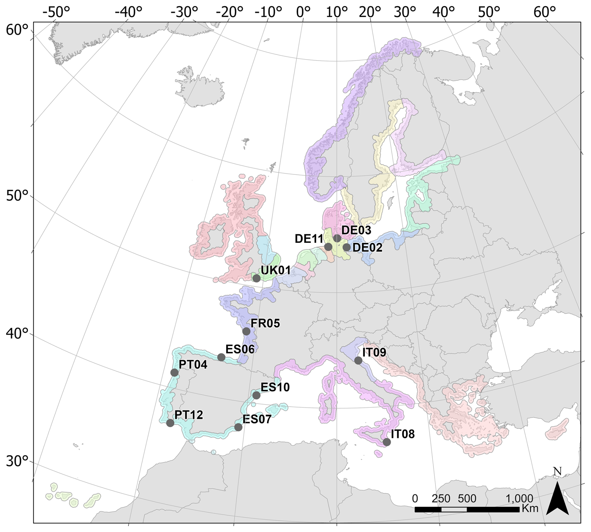
Figure 2 Continental-scale flood units illustrated with colorful polygons and locations of local-scale control cases.

For each unit, flexible topographic meshes were generated, with topographic crests defining the mesh contours (impact zones). Each impact zone was subdivided into impact cells of equal resolution to the DEM. Boundary impact zones, representing points of water entry from the sea, were assigned hydrographs from the closest CTP. Within each mesh, land cover classes were attributed to impact zones based on dominant land-use type, and Manning's roughness coefficients were assigned accordingly, following van der Sande et al. (2003) (see Table S2). Synthetic hydrographs were used to test the numerical stability of the meshes before full simulations.

3.3 Hydraulic simulations

RFSM-EDA simulates flood propagation using a simplified two-dimensional storage cell model that approximates the momentum equation through a diffusive form of the shallow-water equations with local inertia. The computational grid is composed of impact zones, in which Saint-Venant equations are solved. Water depth and mean velocity represent the model outputs provided in each impact cell, yielding flood maps at the same resolution as the input DEM (Gouldby et al., 2008; Jamieson et al., 2012). The representation of coastal defenses lies outside of the scope of the proposed methodology. However, given their role as an important uncertainty source in flood modeling, their influence is evaluated separately in a dedicated sensitivity analysis.

4 Validation

4.1 Approach

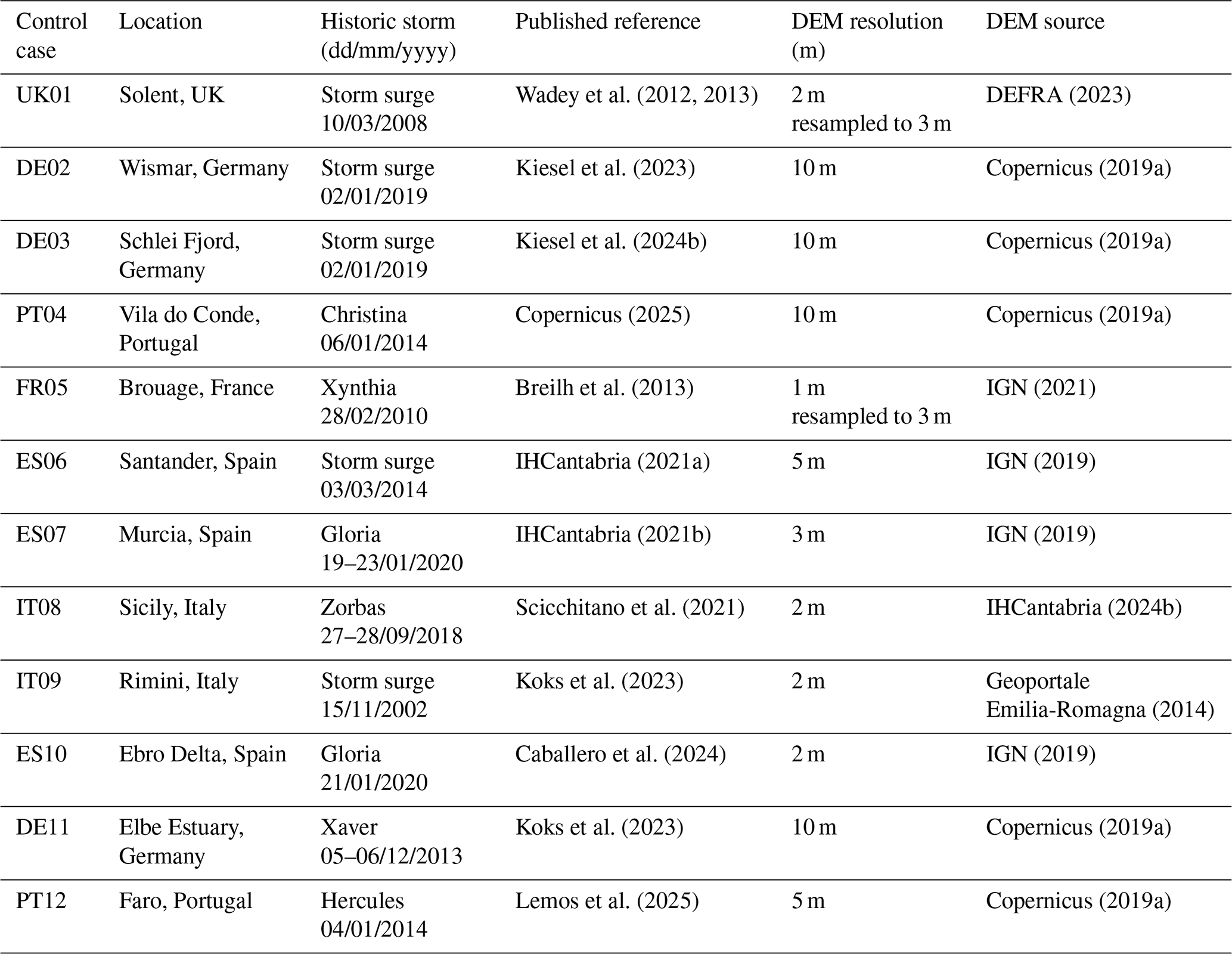
Validation was carried out using 12 local-scale control cases, which also supported the identification of the main sources of uncertainty. These cases were selected based on published studies that compared process-based flood model simulations with observations of real historical flood events across Europe. Table 2 summarizes the selected cases, including their location, the storm event analyzed, the reference publication, and details of the associated high-resolution DEM used. As the source of the high-resolution DEM data used in the control cases varied so did the vertical datum. In cases where the datum information was explicit (e.g., Germany, Portugal, Spain, and France), the appropriate corrections were applied in each case. Otherwise, the geoid was considered as the default reference in order for a vertical correction to be applied. The locations of the control cases are shown in Fig. 2.

Table 2 Local-scale control cases and their respective historic storms, published references used to validate the coastal flood modeling methodology, and high-resolution DEM information adopted in each case.

The methodology was validated by reproducing historical flood events with our modeling framework and comparing results against reference maps from the literature. Validation included both qualitative (visual) comparisons and quantitative analyses using the Critical Success Index (CSI) (Eilander et al., 2023):

$$\begin{array}{}\text{(1)}& \mathrm{CSI}={\displaystyle \frac{F_{\mathrm{sim}}\cap F_{\mathrm{obs}}}{F_{\mathrm{sim}}\cup F_{\mathrm{obs}}}},\end{array}$$

where F_sim is the modeled flooded area and F_obs is observed flooded area. CSI values range from 0 (no agreement) to 1 (perfect agreement). Overestimation occurs when the modeled extent exceeds observations, while underestimation reflects missed flooded areas.

4.2 Validation results

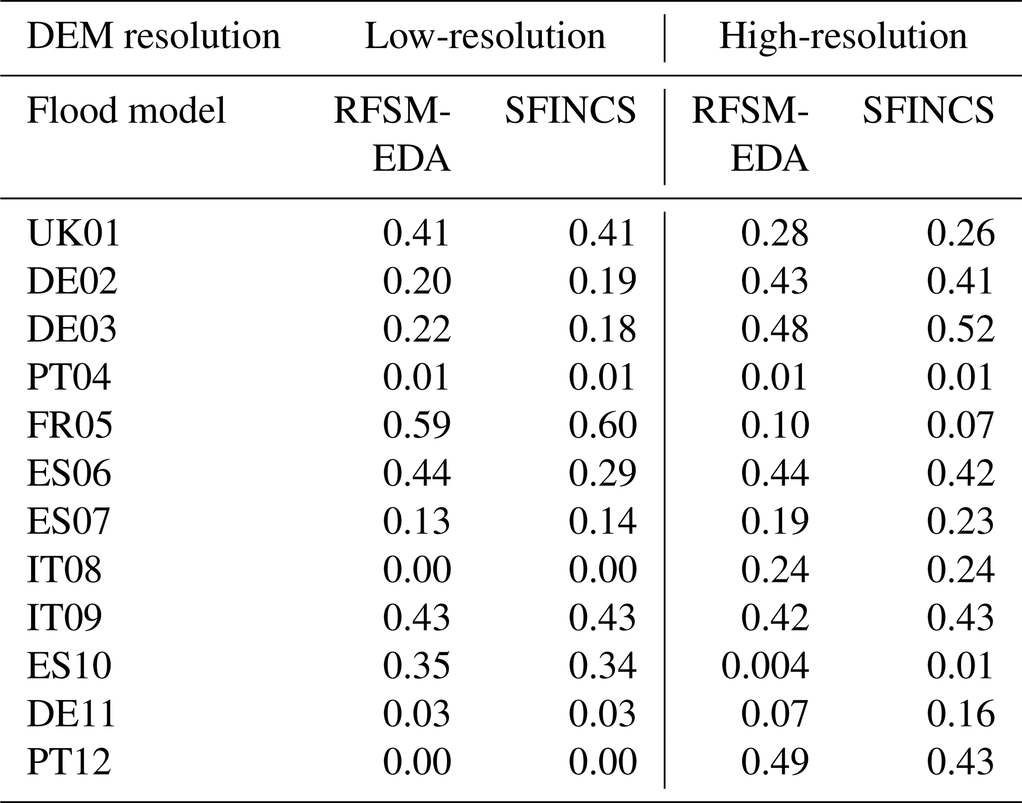
Figure 3 illustrates the reconstructed coastal flooding results using the continental-scale methodology proposed (RFSM-EDA with the 25 m EU-DEM) compared with observed maps. “Hit” denotes true positives (agreement), “false” denotes false positives (overestimation), and “miss” indicates false negatives (underestimation). Table 3 presents the CSI for each case with higher values indicating better agreement between the simulations and the observations.

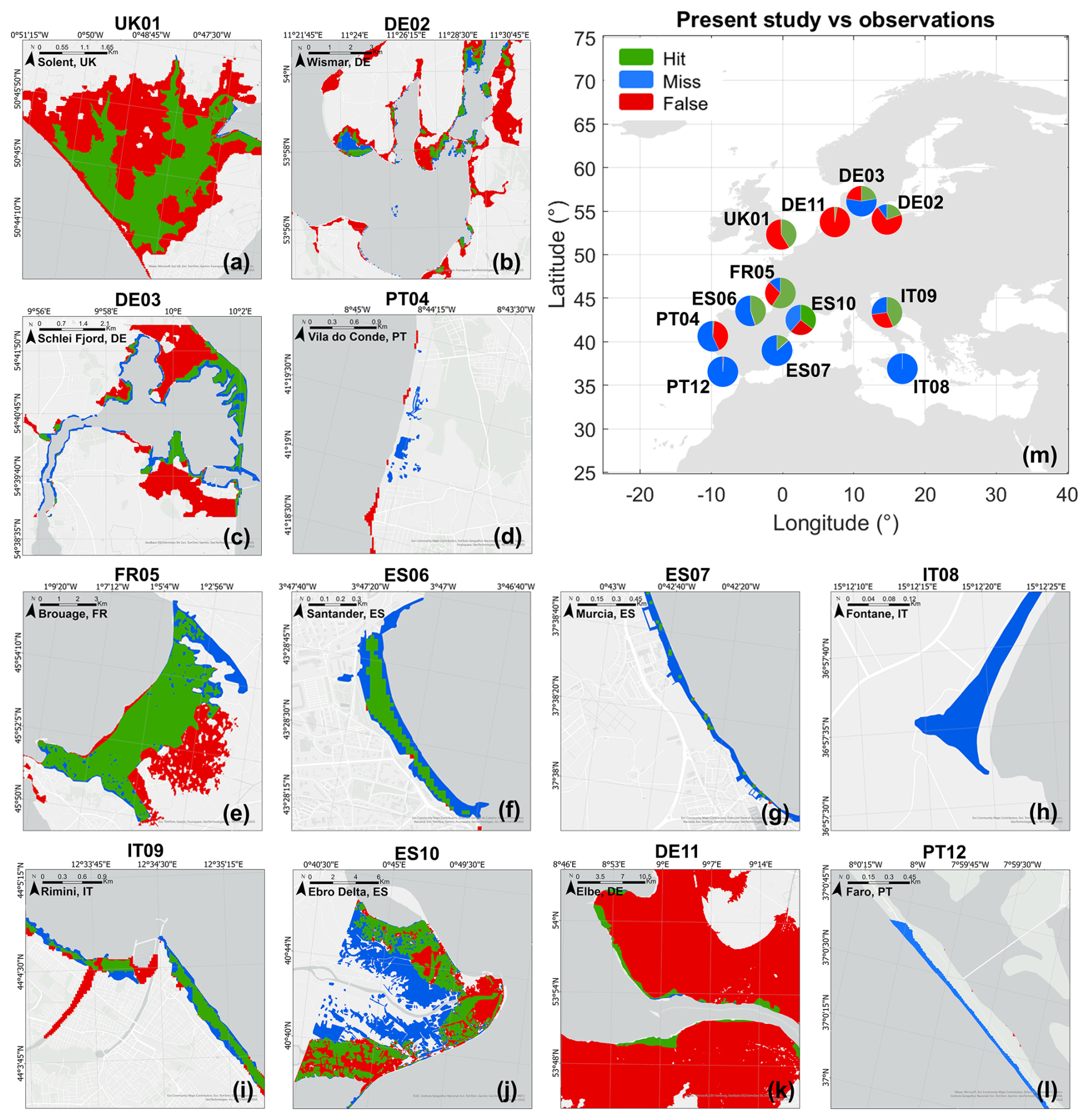
Figure 3 Validation of the methodology. (a–l) Local-scale coastal flooding results from historic storms obtained in the present study compared to observations from previous studies. Results are shown for 25 m DEM and process-based simulations from RFSM-EDA. (m) Proportion of the flood extent which is hit (green), miss (blue), and false (red) for each control case. Note. The overestimation shown as “false” in UK01 (a), DE02 (b), DE03 (c), and DE11 (k) is mainly due to the existence of coastal defenses not considered in our methodology. Basemap data: Esri UK, Esri, TomTom, Garmin, GeoTechnologies, Inc., METI/NASA, USGS | Powered by Esri.

Table 3 Critical success index (CSI) comparing the simulated results in the present study against observations. Results are shown for both DEM resolutions and flood models applied in each local-scale control case.

The most accurate results generally occurred in cases where the model slightly overestimated the observed flood extent, such as UK01 (Fig. 3a), FR05 (Fig. 3e), and IT09 (Fig. 3i). The first two cases are representative of flat floodplains and wetlands, where overestimation is likely related to the smoothing of the terrain in the 25 m DEM and the absence of coastal defenses. For IT09, overestimation likely reflects the influence of the River Marecchia, since small river channels are represented in the 25 m DEM, as well as the neglect of infiltration processes, which would reduce flood extents in reality. A notable exception is ES06 (Fig. 3f), where results were among the most accurate but underestimated observed flooding. This may be attributed to the high Manning roughness coefficient in urban areas, which reduces flood propagation in the model, or the exposure to additional variables such as the infragravity wave.

The least accurate results were generally associated with underestimation and include PT04 (Fig. 3d), ES07 (Fig. 3g), IT08 (Fig. 3h), and PT12 (Fig. 3l). These sites are dominated by sandy beaches and steeper floodplains, either in terms of mean elevation or the proportion of the floodplain lying below 5 m. Such environments may not be well represented in the 25 m EU-DEM, either because its resolution is insufficient to capture narrow beach ridges or because DEM acquisition did not coincide with the date of the historical event, a relevant aspect for dynamic systems such as sandy beaches. Accurate boundary condition definition also proved critical, as the flood model is sensitive to how water is introduced into the system.

In three cases (DE02, DE03, DE11; Fig. 3b, c, and k), reference flood maps were indirectly validated models rather than direct observations. Differences between our results and these references can be explained by key input assumptions. On the one hand, DE02 and DE03 did not include wave setup in their reference maps, whereas our study did. Given the low exposure of both sites to wave action, wave setup is likely not the sole reason for such result. On the other hand, all three reference maps accounted for existing coastal defenses, leading to a smaller observed extent. Overestimation results in UK01, DE02, DE03, and DE11 are similarly explained by the absence of coastal defenses in our model (Kiesel et al., 2023, 2024b; Koks et al., 2023; Wadey et al., 2012). However, even if coastal defenses were included in the DEM, their representation in a flood model presents its own challenges as defense failure mechanisms could in fact result in a larger flooded area than its neglect in the input data. These aspects are further addressed in the sections on Confidence index and Sensitivity analysis of the influence of coastal defenses.

4.3 Sensitivity analyses using control cases

Beyond the validation of the methodology, the control cases were used for three sensitivity analyses (Fig. 4):

1. Flood model selection – RFSM-EDA (Jamieson et al., 2012) was compared with SFINCS (Leijnse et al., 2021). Both are process-based models capable of reproducing flood maps at the same resolution as the DEM.

2. DEM resolution – results with the 25 m EU-DEM were compared to those using the highest available resolution DEM for each case. While the 25 m EU-DEM is considered high-resolution at the continental scale, it is treated as low-resolution in the control cases, as it is compared with even higher-resolution DEMs.

3. Foreshore slope approximation – the Sunamura (1984) method was compared with slopes derived from high-resolution topo-bathymetric data.

Together, these tests supported the identification of the most important sources of uncertainty across the different methodological steps.

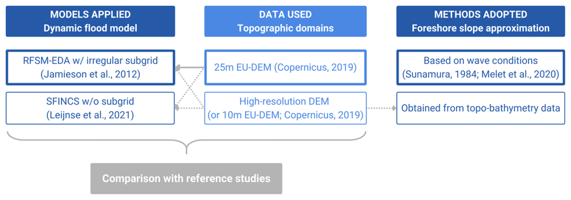
Figure 4 Methodology applied to local-scale control cases. The boxes marked with thick lines show the methodology applied at the European scale while the dashed lines indicate all the combinations of steps performed in the sensitivity analyses of the control cases.

4.3.1 Sensitivity analysis: flood models

Comparison between RFSM-EDA and SFINCS results (Table 3) shows broad consistency. Of 24 simulations (12 cases × 2 models), 8 produced identical CSI values, 9 favored RFSM-EDA, and 7 favored SFINCS. RFSM-EDA tended to perform better in steeper areas with higher foreshore slopes and mean elevations, while SFINCS performed better in flat and large floodplains. At high resolution both models produced equally accurate results, but at lower resolution, RFSM-EDA generally outperformed SFINCS. Overall, this consistency indicates that the modeling approach adopted at continental scale is robust.

4.3.2 Sensitivity analysis: DEM resolution

Comparisons of DEM resolutions indicated that higher resolution does not always yield better results. Of the 24 simulations (12 cases × 2 resolutions), 13 favored higher-resolution DEMs, 7 favored lower resolution, and 2 were equal (Table 3). High-resolution DEMs improved results in sites with higher mean elevation or sandy beaches (e.g., DE02, DE03, ES06, IT08, ES07, PT12). By contrast, in flat wetlands (e.g., UK01, FR05, ES10), lower-resolution DEMs performed better, likely because smoothing better represents broad floodplain features. These results suggest that large-scale applications can adequately capture flooding in flat coastal plains even with coarser DEMs, while finer resolution is more critical in complex terrains.

4.3.3 Sensitivity analysis: foreshore slope

Foreshore slope is one of the main uncertainty sources in coastal flooding studies that include wave contributions. Therefore, validating the approach adopted here is crucial to ensure its suitability at larger scales. Figure 5 compares the foreshore slopes estimated with the Sunamura (1984) formulation against those obtained with a traditional method across all control cases.

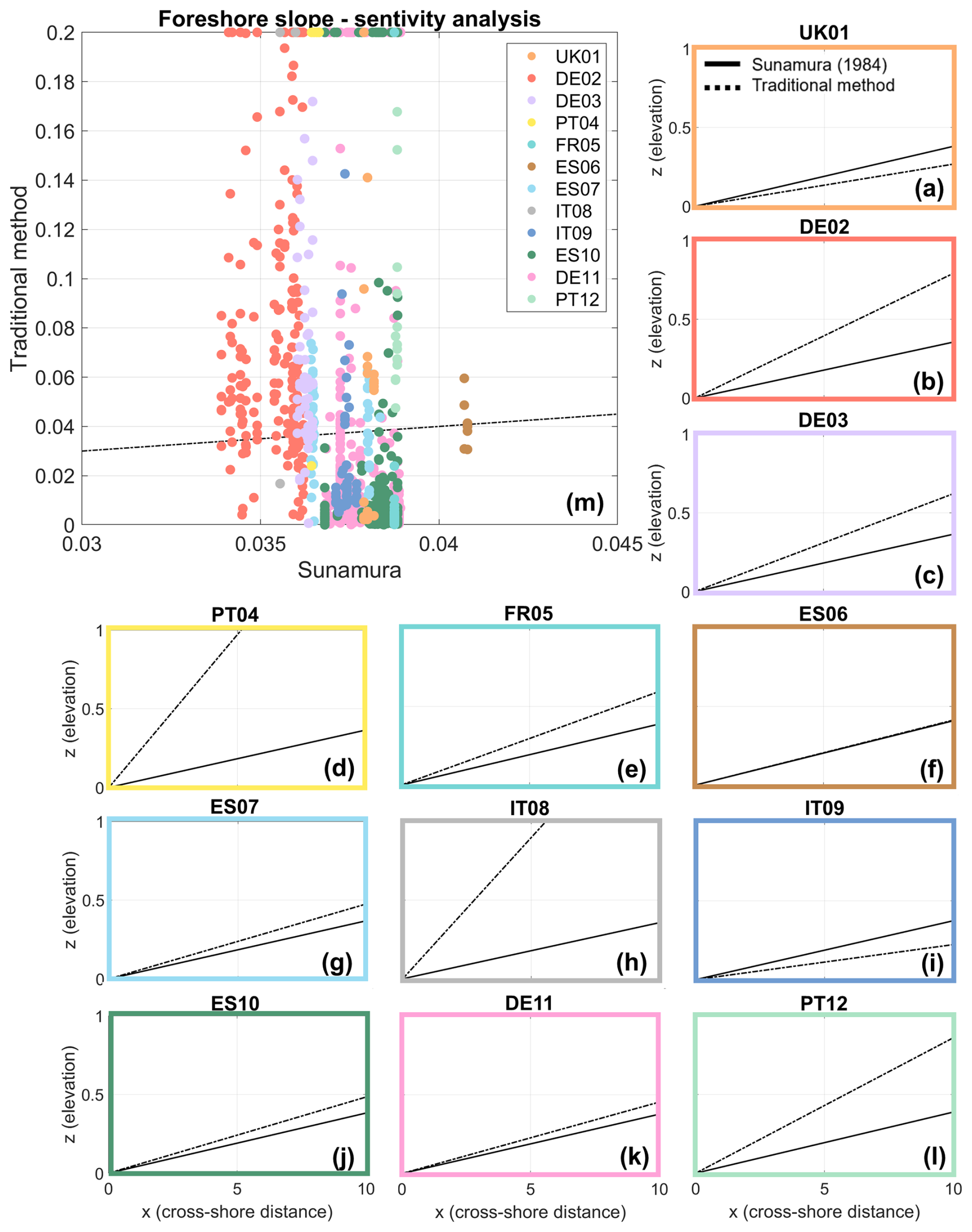
Figure 5 Sensitivity analysis of the foreshore slope approximation. (a–l) Comparison of mean foreshore slopes resulting from the Sunamura (1984) approach and the traditional method per control case. (m) Direct comparison of results per points in each control case. Dashed line indicates a 1 : 1 result.

The Sunamura formulation estimates foreshore slope as a spatially and temporally variable function of wave conditions at each CTP. By contrast, the traditional method derives slopes from high-resolution DEM profiles, calculated as the intertidal slope between the mean low and high tides at each site.

Overall, the two methods show good agreement, with notable exceptions in PT04 (Fig. 5d) and IT08 (Fig. 5h). PT04 represents a long sandy beach that is absent from the 10 m Copernicus DEM, producing unrealistic cliff-like slopes. IT08 is a pocket beach too small to be adequately resolved by the DEM. These cases illustrate that the reliability of the traditional method strongly depends on the quality of the high-resolution DEM available.

In most of the remaining cases (except UK01, Fig. 5a, and IT09, Fig. 5i), the traditional method produced higher slope values than the Sunamura approach. Interestingly, these cases span a wide range of coastal types, from sandy beaches and wetlands to urban beaches and flat floodplains. The best agreement occurred in ES06 (Fig. 5f), where the high-resolution DEM included topo-bathymetry information, allowing for a more precise slope estimate.

Figure 5 summarizes results across all profiles and CTPs, with a clear concentration of points along the 1 : 1 line, indicating close agreement between both approaches. Taken together, these findings show that the Sunamura (1984) formulation is a conservative but robust method that performs well across diverse coastal settings, making it suitable for application at continental scale. Given that the traditional method requires high-resolution topo-bathymetric data, which is not consistently available across Europe, the Sunamura approach represents a practical and sufficiently accurate alternative for defining foreshore slopes.

4.4 Confidence index

Relationships between validation results and the physical characteristics of each control case allow us to infer where flood maps are more or less reliable. As described above, coastal flood estimates tend to be more robust in flat areas with large proportions of water bodies, while results are less reliable in regions characterized by pocket beaches or coastal defenses.

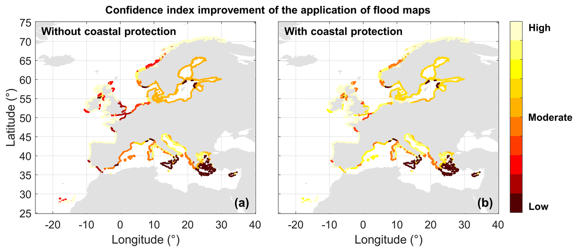
Figure 6 Spatial distribution of coastal flooding confidence index based on the validation of the methodology through control cases without (a) and with (b) standard levels of coastal protections. Note. This analysis does not consider the influence of coastal protection on flooding itself nor does it include coastal flooding estimations.

Based on these insights, we developed a confidence index for coastal flood projections (Fig. 6a). This index was generated through manual clustering, with each control case acting as a centroid. CTPs were then assigned to the most similar control case according to five physical characteristics: (i) proportion of floodplain below 5 m elevation, (ii) relative extent of water bodies within land use, and (iii–v) the average relative contributions of astronomical tide, storm surge, and wave setup at the TWL peak moment.

The highest confidence values are observed in tide-dominated areas with relatively simple coastal configurations, such as the Bay of Biscay, and sections of the Norwegian coast. The lowest values appear in the North Sea, including parts of the UK, Belgium, and the Netherlands, as well as in the southeastern Mediterranean, where more complex hydrodynamic regimes and irregular coastlines dominate. Figure 6b incorporates the minimum standards of coastal protection from the COASTPRO-EU database (van Maanen et al., 2025). In this case, confidence increases along well-defended coasts such as the UK and the Netherlands, where coastal defenses are extensively documented. However, low confidence persists in Greece, Cyprus, and southern Italy, likely due to the prevalence of pocket beaches, which are not well represented in the DEM (as illustrated in IT08).

Although this index does not directly reflect flood extents or the protective effect of coastal defenses, it provides a first-order measure of where continental-scale flood projections are more or less reliable. It also highlights regions where incorporating coastal defense data could substantially improve confidence in future modeling efforts.

5 Results

Pan-European coastal flooding simulations are presented in terms of maximum flooded areas (MFA) or relative MFA, expressed as a proportion of the overall floodplain area. Sensitivity analyses were conducted to assess the influence of different flood modeling approaches (static vs. dynamic), hydrograph shapes (triangular vs. smooth-shaped), storm type scenarios, and coastal defenses on coastal flooding. These analyses were performed at multiple scales: the entire study area, regional (Atlantic coast, Baltic Sea, and Mediterranean Sea), national, and NUTS2 (major socioeconomic regions defined by the European Commission).

5.1 European coastal flooding

Figure 7 shows the MFA resulting from smooth-shaped hydrographs, based on the location-specific average TWL storm shape, applied to the dynamic flood model RFSM-EDA for a 100-year TWL composite storm type event, without considering coastal defenses. The MFA for Europe is 47 871 km². The spatial distribution of flooding reflects a combination of two key factors: topographic characteristics and peak water levels.

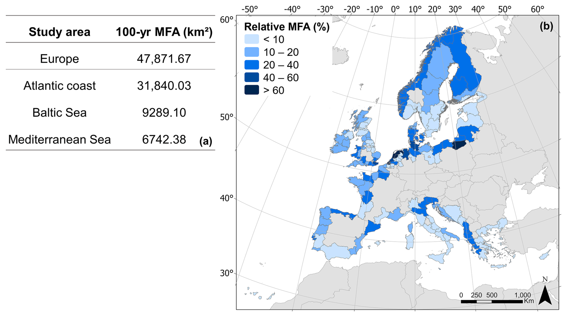
Figure 7 Coastal flooding results for a 100-year TWL event. (a) Maximum flooded area (MFA; km²) considering the entire study area and European regions. (b) Spatial distribution of relative MFA (%), aggregated per NUTS2 to facilitate the interpretation of results.

The most affected areas, those with the highest proportions of the floodplain being inundated, coincide with smoother topography and flatter floodplains, represented by DEMs with large areas below 5 m. For example, the southeast North Sea contains extensive floodplains, more than half of which lie below 5 m. A similar pattern occurs in parts of the Adriatic Sea, where floodplains are flat and the mean elevation is only 4.62 m.

By contrast, the least affected areas coincide with steeper floodplains and lower 100-year TWLs. Examples include the Ionian Sea and the central Baltic, where mean 100-year TWLs are 0.79 and 1.47 m, and mean DEM elevations are 7.80 and 8.04 m, respectively.

Additional physical factors also influence flooding exposure, particularly coastal morphology. Large rivers and estuaries act as pathways for flood propagation inland, as seen along the Atlantic coast of France and parts of the United Kingdom. Extensive flood extents are also found in regions with wetlands and mudflats, such as the Wadden Sea and Arkona Basin. Conversely, rocky cliffs and bedrocks coasts act as natural barriers against extreme water levels, as observed in the Aegean Sea and the Sea of Crete.

Country-level relative MFA estimates for a 100-year TWL event are provided in the Supplement (Table S3).

5.2 Sensitivity analysis of the modeling approach

A comparison between static and dynamic flood models is essential to determine whether, and under what conditions, the commonly used bathtub approach can serve as a viable alternative to more computationally demanding process-based models. Table 4 presents MFA values for the entire study area and for each European region, using a 100-year TWL event under both static and dynamic approaches.

Table 4 Maximum flooded area (km²) resulting from a 100-year TWL with a bathtub approach and with RFSM-EDA for the entire European floodplain and per European region.

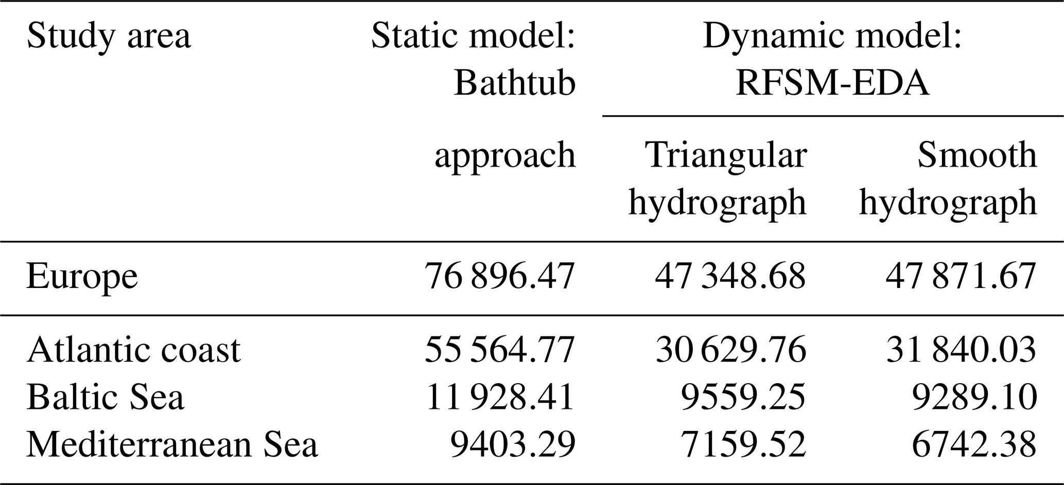
For the European coastline as a whole, 36.8 % of the floodplain (i.e., area below 15 m of elevation and hydrologically connected to the sea) is inundated with the static model, whereas the dynamic model RFSM-EDA, driven by smooth hydrographs, reduces the relative MFA to 22.9 %. This implies that the static approach exposes an additional 13.9 % of the European floodplain to flooding during a 100-year TWL event.

Regional differences are pronounced. Along the Atlantic coast, the discrepancy between static and dynamic models reaches 21.1 %, while in the Baltic and Mediterranean Seas the differences are smaller, at 4.6 % and 6.9 %, respectively. This highlights the Atlantic coast as the region most sensitive to the use of static modeling. The Atlantic is characterized by extensive flat floodplains and gentle terrain, conditions under which the static assumption that all low-lying areas are flooded is unrealistic, as it ignores the limited energy and attenuation of floodwaters. By contrast, in the Baltic and Mediterranean Seas, steeper and more complex topography constrains the extent of flooding in the static model. At the same time, longer storm durations in these regions enhance inland flood propagation in the dynamic simulations, partially offsetting the difference.

Country-level relative MFA results are provided in the Supplement (Table S3). Once again, the greatest discrepancies between static and dynamic models occur in low-lying regions with large floodplains. For example, the differences are 25.7 % in Belgium and 29.6 % in the United Kingdom, both characterized by broad, flat coastal areas. By contrast, the differences are only 1.4 % in Finland and 2.8 % in Sweden, where rugged coastlines with cliffs and fjords and higher mean floodplain elevations limit flood extent.

5.3 Sensitivity analysis of the hydrograph shape

Besides topographic characteristics, peak water level, and storm duration, hydrograph shape also influences flood extent through its direct effect on the volume of water entering the system. Table 4 presents MFA values for the entire study area and for each European region using triangular and smooth-shaped hydrographs for a 100-year TWL event. Figure 8 presents relative MFA results for a 100-year TWL event per country under each modeling approach for a composite storm type scenario.

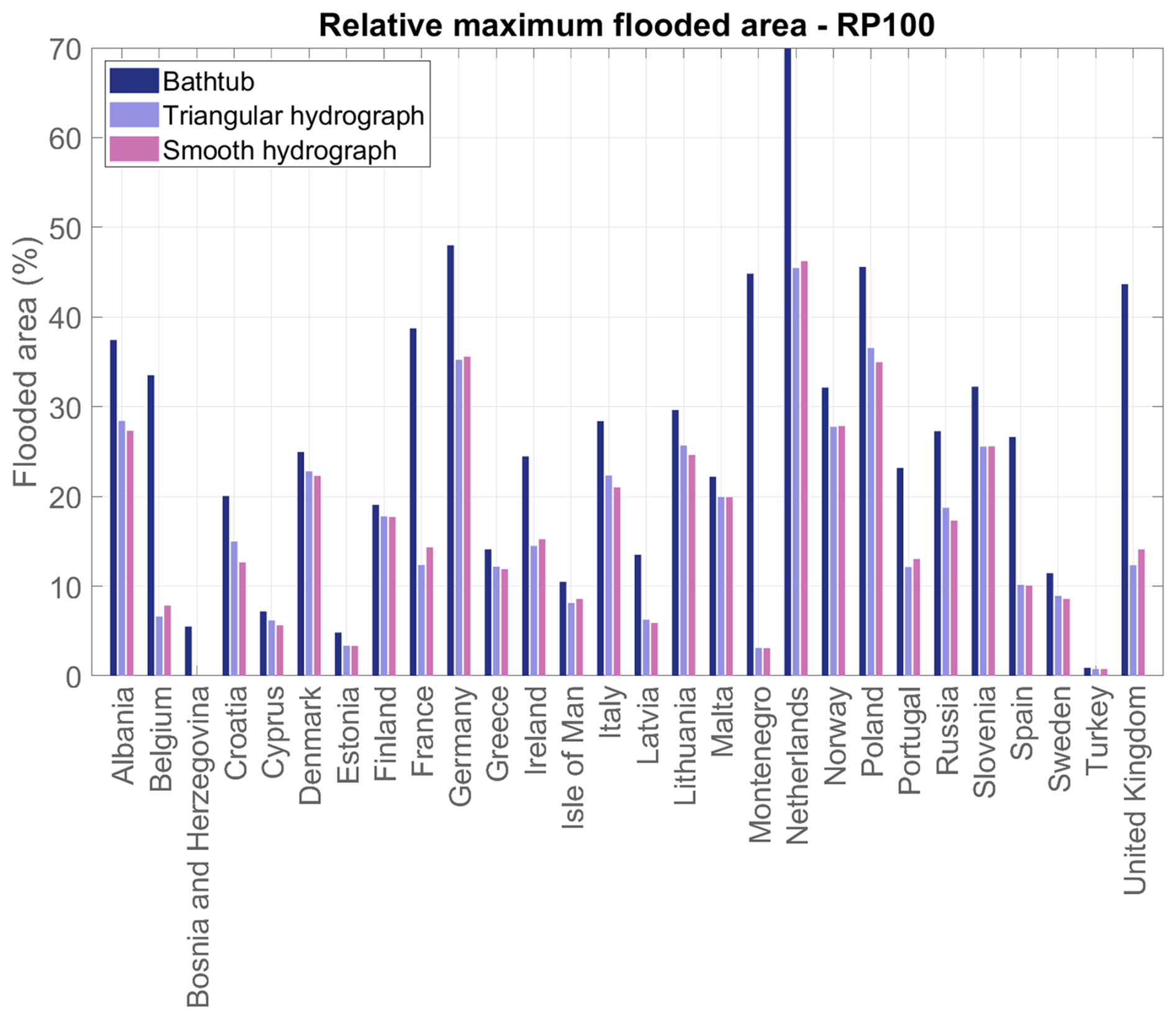
Figure 8 Relative maximum flooded area (%) per country for a 100-year TWL (RP100). Results are shown for the bathtub approach, dynamic flood modeling with a triangular hydrograph, and dynamic flood modeling with a smooth hydrograph. Values are relative to each country's own floodplain area.

At continental scale, the use of smooth hydrographs, as opposed to the commonly used triangle ones, leads to a 0.25 % increase in MFA. Regional responses, however, differ. Along the Atlantic coast, smooth hydrographs increase MFA by 1.08 %, whereas in the Baltic Sea and Mediterranean Sea MFA is reduced by 0.47 % and 1.08 %, respectively. Two mechanisms explain these patterns. First, increases in MFA occur in regions with higher 100-year TWLs. Even small differences in storm shape translate into significantly larger water volumes, altering the boundary conditions of flood events, as observed in France and the United Kingdom. Second, the type of storm influences how smoothing affects MFA. Along the Atlantic coast, where storms follow a tidal cycle, hydrographs naturally exhibit a sinusoidal shape. For the same peak level and duration, a triangular hydrograph is almost always smaller than its smooth, sinusoidal counterpart, resulting in larger MFA when smooth shapes are used. Conversely, in regions where storm surge and wave setup play a stronger role, hydrographs display diverse forms, ranging from single sharp peaks to multiple oscillations of varied magnitudes. In these cases, smoothing can either decrease the water volume, as in Croatia and Poland, or have little to no effect, as in Malta and Turkey.

On average, MFA differences between triangular and smooth hydrographs remain below 3 % across most of the study area, suggesting that the influence of hydrograph shape is limited but non-negligible. The largest differences occur in sheltered parts of the Mediterranean, such as Croatia and Cyprus, where wave setup contributions are high and hydrograph shapes differ most from the triangular assumption. In contrast, tide-dominated storms approximate sinusoidal curves and surge-dominated storms resemble single peaks, both of which are closer in shape to triangular hydrographs.

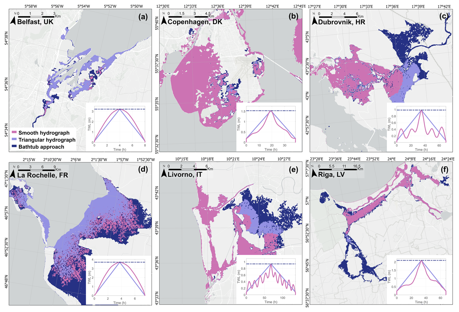
Figure 9 Comparison of flood extent for a 100-year TWL resulting from the bathtub approach and the dynamic process-based RFSM-EDA flood model with both a triangular and a smooth-shaped hydrograph. Hydrographs are represented for each respective example. Basemap data: Esri UK, Esri, TomTom, Garmin, GeoTechnologies, Inc., METI/NASA, USGS | Powered by Esri.

Figure 9 illustrates six examples comparing static flood modeling (bathtub approach), dynamic modeling with triangular hydrographs, and dynamic modeling with smooth hydrographs. In all cases, static models overestimate flood extent, though the magnitude of overestimation varies. Differences between triangular and smooth hydrographs are minor in Belfast, Copenhagen, and Riga (Fig. 9a, b, and f), where both hydrograph shapes are very similar. La Rochelle also exhibits similar hydrograph shapes, but the flat terrain amplifies the effect of even small changes in water volume, resulting in noticeable differences in flood extent (Fig. 9d). The largest discrepancies occur in Dubrovnik and Livorno (Fig. 9c and e), both in the Mediterranean, where wave influence is high. Here, smooth hydrographs show strong fluctuations that significantly decrease water volume compared to triangular ones, leading to smaller flood extents.

5.4 Sensitivity analysis of the storm types variability

The distinction between storm types leading to coastal flooding reflects the spatial variability of marine dynamics across the study area, as each type has its own distribution and frequency. For instance, storm surge–dominated ST A events occur predominantly in the Baltic Sea, whereas astronomical tide–dominated ST B events are more frequent along the Atlantic coast. The remaining storm types show more scattered patterns: ST C, which is tide-leaning, resembles ST B, while ST D, which is surge-leaning, resembles ST A. The Mediterranean Sea shows the clearest differences, with most events being mixed, resulting in higher frequencies of ST C than ST B, and of ST D than ST A. Beyond spatial patterns, storm type also influences the characteristics of flood events. For example, surge-dominated events are estimated to last longer than tide-dominated events, which in turn may prolong the duration of flooding.

Table 5 Relative maximum flooded area (%) resulting from a 100-year TWL under different storm types for the entire European floodplain and per European region. Values are shown relative to each floodplain area to facilitate the comparison of results.

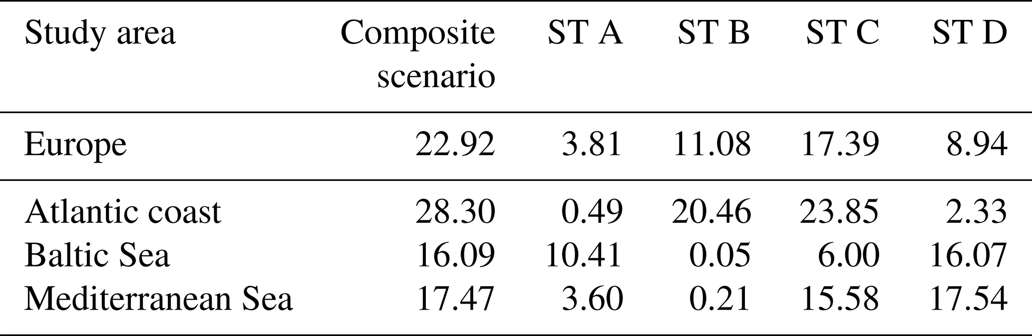
Table 5 shows the relative MFA for the entire study area and per European region for different storm types as well as for a composite storm scenario, using the dynamic flood model and smooth-shaped hydrographs. Regional differences emerge. On the Atlantic coast, the largest MFA occurs under the composite scenario, while surge-dominated ST A produces very small flooded areas. This suggests that tide-dominated and tide-leaning storms (ST B and ST C) alone do not generate the most extreme floods while surge-dominated ST A produces limited flooding because it neglects tidal contributions in a region with large tidal amplitudes. In the Baltic Sea, the largest MFA occurs under both the composite scenario and surge-leaning ST D, while tide-dominated ST B produces negligible flooding. The same pattern is observed in the Mediterranean Sea, where tide-dominated ST B results in the smallest MFA. Both semi-enclosed seas are microtidal environments, where tide-dominated storms are rare and less relevant. Interestingly, in the Mediterranean Sea the largest MFA is not produced by the composite scenario but by surge-leaning ST D. This reflects the strong influence of waves in the region, since otherwise surge-dominated ST A would be expected to produce more extensive flooding.

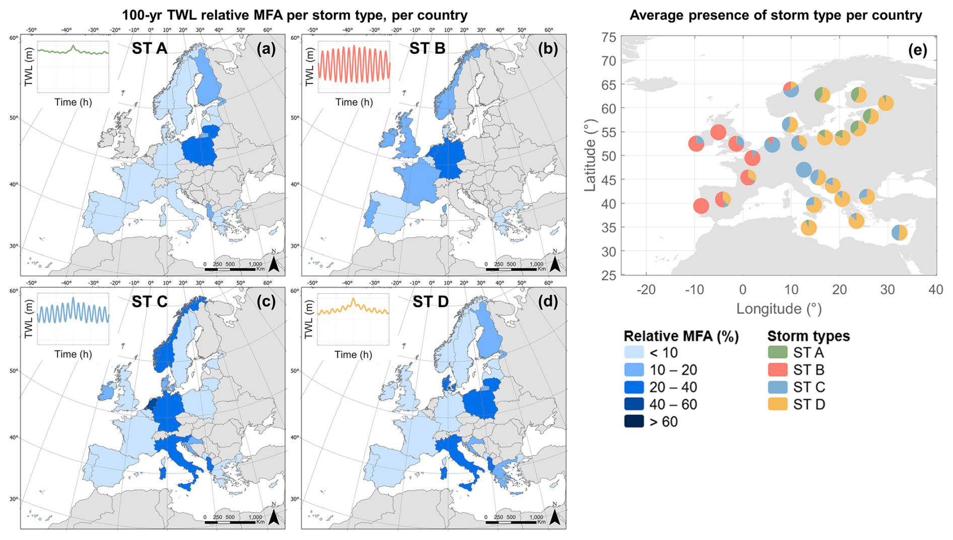
Figure 10 Relative maximum flooded area ( %) per country for a 100-year TWL, per storm types: (a) ST A, (b) ST B, (c) ST C, and (d) ST D. Results are shown for dynamic flood modeling with smooth-shaped hydrographs. Values are relative to each country's own floodplain area. (e) Average presence of storm type per country.

Figure 10 illustrates the relative MFA by storm type for a 100-year TWL event, per country. Results mirror the diverse topographic and marine conditions across Europe. In some cases, specific storm types lead to greater MFA than the composite scenario (see Table S3). For example, in Malta and Lithuania, the largest MFA occurs under surge-dominated ST A (Fig. 10a). In the Netherlands, Germany, and Turkey, the greatest MFA occurs under mixed, tide-leaning ST C (Fig. 10c). In Croatia, Italy, Latvia, and Poland, it occurs under mixed, surge-leaning ST D (Fig. 10d). Meanwhile, France, Greece, Norway, and Spain show the largest MFA under the composite scenario. These outcomes reflect the diversity of coastal settings. The large spatial extent of Norway, the split of France and Spain between Atlantic and Mediterranean coasts, and the many islands of Greece contribute to complex climatologies and diverse topographies that influence the results.

Within individual countries, storm type can produce significant regional variability in flood projections. For example, Germany spans both the North Sea and the Baltic Sea, each with distinct characteristics. Along the North Sea, high 100-year TWLs combine with broad, flat floodplains to produce extensive flooding, particularly under tide-dominated scenarios. Along the Baltic, storm durations are longer, increasing exposure time to extreme water levels. As a result, under a tide-dominated ST B scenario, Germany's North Sea coast floods by 34 %, compared to just 1 % along the Baltic coast. Under a surge-leaning ST D event, the North Sea coast floods by only 3 %, while the Baltic coast floods by 16 %. Similar regional contrasts are observed in Denmark, France, Spain, Italy, and Sweden. Such information provides valuable evidence for directing emergency resources and developing coastal management strategies.

5.5 Sensitivity analysis of the influence of coastal defenses

Figure 11 presents relative MFA values without coastal defenses and with minimum and maximum standards of coastal protection based on COASTPRO-EU (van Maanen et al., 2025). Results are aggregated at the NUTS2 level. Under a 100-year TWL event, MFA for Europe decreases from 47 871 km² (no defenses) to 28 914 km² (13.9 % of the floodplain) when applying the minimum protection standard, and further to 18 848 km² (9.0 %) under the maximum standard. These reductions show strong spatial variability. Some countries have no available data on coastal protection, while others, such as the Netherlands, are comprehensively protected by dune systems designed to withstand events with return periods ranging from 1250 to 10 000 years (Kind, 2014).

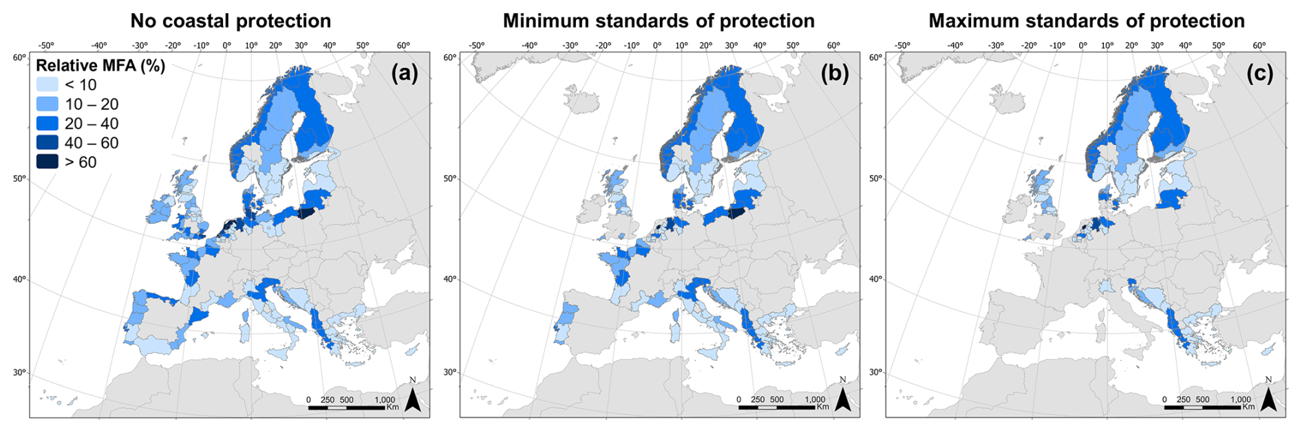
Figure 11 European spatial distribution of 100-year TWL flood hazards without coastal protection (a) and with minimum (b) and maximum (c) standards of coastal protection using a dynamic flood model with smooth-shaped hydrographs and a composite storm type scenario. Results are shown as relative MFA in regards to the floodplain area of each NUTS2. Standards of coastal protections were obtained from the COASTPRO-EU database (van Maanen et al., 2025).

Our results can be compared with previous studies. Vousdoukas et al. (2016), who also used a dynamic flood model with coastal protections, reported higher MFA values. Relative to their study, our results are 6.2 % lower under the minimum protection standard and 62.9 % lower under the maximum standard. Besides the use of a more recent and updated dataset of coastal protection standards (i.e., COASTPRO-EU vs. FLOPROS of Scussolini et al., 2016), these differences likely reflect both the higher resolution of our analysis (25 m vs. 90 m flood map resolution) and our characterization of wave setup. While Vousdoukas et al. (2016) applied a uniform wave setup of 0.2Hs with offshore wave conditions, we used a semi-empirical formulation based on nearshore wave conditions and spatially varying foreshore slopes, which provides more detailed boundary conditions.

When comparing our static model results with Groenemeijer et al. (2016), who also accounted for coastal defenses, our MFA is 45.3 % larger under the minimum protection standard and 14.7 % larger under the maximum standard. These differences are attributable to our explicit inclusion of wave effects, besides the higher resolution DEM used. Even larger discrepancies are found when comparing with Paprotny et al. (2018). Their protected scenarios, produced with a static flood model that neglected waves and used a 100 m DEM, result in 59.3 % and 36.4 % less MFA than our static model results under minimum and maximum protection standards, respectively.

The spatial distribution of relative MFA values without coastal defenses and with minimum and maximum protection standards, using a static flood model, is provided in the Supplement (Fig. S1).

6 Discussion and Conclusions

In this study, we presented a methodology to assess coastal flood impacts at large scale. This was achieved by applying a 25 m resolution DEM and location-specific hydrographs of extreme TWL events to the process-based flood model RFSM-EDA. The methodology was validated through the reconstruction of 12 historical flood events using local-scale control cases. Although the validation exercise did not produce equally strong results across all cases, it allowed us to explain the observed performance, identify key sources of uncertainty, and highlight methodological steps with potential for improvement. The key challenges of large-scale coastal flooding studies, from preparing boundary conditions to applying flood models, were analyzed and confirmed as important sources of uncertainty in both continental- and local-scale analyses.

Our results show that coastal flood extent depends on both topographic and storm-related characteristics. Storm characteristics include peak water level, storm duration, and storm shape. While static flood models account for topography and peak water levels, only dynamic models can capture the influence of storm duration and shape on flood extent. Consistent with previous findings, our comparisons reveal that static models systematically overestimate flood extent, particularly in flat areas. The additional insight provided here is the quantification of the influence of storm shape and storm type, representing a further advancement in large-scale dynamic flood modeling.

Table 6 European maximum flooded area (km²) resulting from a 100-year TWL in different studies.

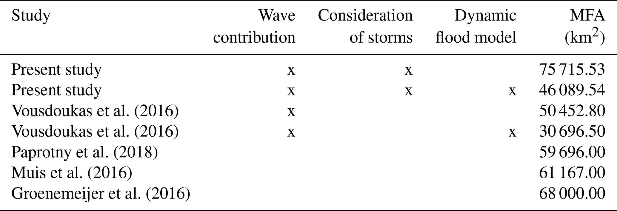
Note: MFA results should be interpreted with caution when compared across studies, as differences in spatial domain and underlying data coverage can affect the reported values; comparisons are therefore indicative rather than directly comparable.

When comparing the 100-year TWL MFA obtained here with other studies (Table 6), differences can be attributed to three main factors: (1) the flood modeling approach; (2) marine boundary conditions; and (3) data resolution. First, regarding flood modeling approaches, both Vousdoukas et al. (2016) and the present study found that European MFA estimates from static models were 38 %–39 % larger than those from dynamic models. The similarity of these values suggests that neither the specific dynamic model used (LISFLOOD vs. RFSM-EDA) nor the DEM resolution (90 m resolution vs. 25 m resolution) alone explains the influence of the modeling approach. Second, when focusing on static model results, our study yields 12 % more flooded area than Groenemeijer et al. (2016), 21 % more than Muis et al. (2016), and 22 % more than Paprotny et al. (2018), all of which excluded wave contributions. Third, DEM resolution affects the results of hydrodynamic flood simulations, but its influence is not straightforward. For instance, even though Muis et al. (2016) used the coarsest DEM (1 km), it did not show the largest divergence in MFA when compared to this study. These discrepancies highlight the role of other factors such as input data, modeling approach, and treatment of coastal defenses, which are not fully captured in this comparison.

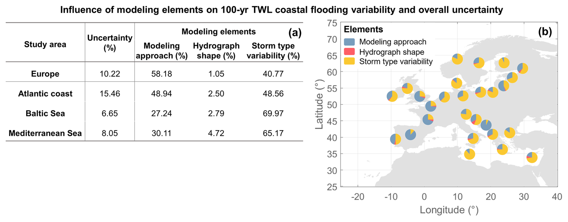
Figure 12 Influence of modeling elements (modeling approach, hydrograph shape, and storm type variability) on 100-year TWL coastal flooding variability and overall flood map uncertainty. Results are shown for (a) the entire study area and per European region as well as (b) per country.

A summary of our sensitivity analyses shows that flood map uncertainty at the European scale (10.2 %) can be partitioned into contributions from the modeling approach (58.2 %), storm type variability (40.8 %), and hydrograph shape (1.0 %) (Fig. 12). Regarding the modeling approach, results confirm that topographic characteristics strongly influence sensitivity. For example, the Atlantic region, characterized by extensive, flat floodplains, proved most sensitive to model choice. Terrain type and land use also play a role, since Manning's roughness coefficients influence flood propagation in dynamic models. Floodplains with larger proportions of rural and urban areas showed greater sensitivity to the modeling approach, as higher roughness values limit flood spread and increase the differences between static and dynamic models.

Storm type variability proved most important in the semi-enclosed Baltic and Mediterranean Seas. Storm types influence coastal flooding in two ways. First, regions with more diverse storm regimes are more sensitive to storm type variability. For example, the Atlantic coast is dominated by tide-dominated ST B, so most events behave similarly. In contrast, the Baltic and Mediterranean Seas feature more diverse storm regimes, producing a wider range of flood outcomes. Second, storm type affects the duration of coastal flooding. Storm durations are anticipated to be shorter with tide-dominated ST B, followed by tide-leaning ST C, surge-leaning ST D, and surge-dominated ST A events. Longer storm durations extend the time that water flows into floodplains, even at low velocities, thereby increasing flood extent (Höffken et al., 2020). Consequently, surge-dominated storms can lead to more extensive flooding through longer persistence, while tide-dominated storms may inundate large, flat areas.

Beyond the quantified sources of uncertainty, additional limitations were identified. From the validation analysis, we infer that many uncertainties are inherent to working at large scales. The most important are related to data (especially DEMs) and methods (e.g., foreshore slope and wave setup parameterizations). Similar issues were identified by Le Gal et al. (2024), who showed that lower-resolution grids tend to exaggerate flood extent by smoothing small protective features. In our case, high-resolution DEM acquisition dates did not always match the timing of historical events, and vertical datums were sometimes unknown. Furthermore, important processes such as storm-induced coastal erosion were not included, and in some cases, existing coastal defenses were neglected.

The neglect of human adaptation, particularly coastal defenses, represents the largest source of bias in large-scale flood risk assessments (Hinkel et al., 2021). Unlike other limitations, this can be partly addressed by post-processing flood maps within risk frameworks that incorporate defense data. Both our confidence index and sensitivity analysis of coastal defenses demonstrate that including defense information improves results without the need to regenerate flood maps. Flood extent varies between 9 % and 22.9 % of the European floodplain depending on the assumed level of coastal protection, with the inclusion of defenses reducing flood extent by 40 %–61 % relative to the undefended case and corresponding to an uncertainty range of 13.9 % attributed solely to the treatment of coastal defenses. However, available coastal protection databases remain coarse, outdated, and inconsistent with the resolution of flood maps, as they provide information only at the NUTS2 level. Such datasets (e.g., COASTPRO-EU) typically reflect nominal or official standards of protection, which can be substantially lower in practice due to inadequate maintenance, deterioration, or changes in the probability of extreme water levels (Paprotny et al., 2025). As a result, flood extents can be highly sensitive to protection-level assumptions and in some cases dominate the overall uncertainty in large-scale flood mapping. Moreover, existing approaches used to incorporate coastal defenses often overlook interactions between neighboring NUTS2 regions. Nonetheless, such analyses highlight the importance of considering existing defenses and the potential to reduce uncertainty by systematically incorporating them.

Large-scale studies necessarily rely on assumptions and simplifications to achieve consistency across vast areas. This introduces uncertainty into input data and model configurations. For example, the foreshore slope approximation used does not differentiate limited or absent intertidal zones, the wave setup formulation adopted was parameterized, and DEMs included permanent waterbodies. Complex coastal environments such as estuaries and island-rich regions introduce further challenges, since the closest CTP may not represent true boundary conditions. These limitations underline that results should not be used directly for local-scale interventions or adaptation planning. Local applications require higher-resolution data and inclusion of additional processes, such as infragravity waves in exposed coasts or detailed foreshore slope estimates for narrow and pocket beaches.

Beyond the previously discussed sources of uncertainty and considering the limitations identified in the study, future research directions are identified for large-scale coastal flood assessment methodologies. First, even though this study treats the entire study area in a systematic way focused on overwashing, the processes that influence coastal flooding vary. For example, dune erosion, berm overtopping, or dike breaching can significantly alter the flood propagation and extent (Nicholls et al., 2015). Therefore, further efforts are needed to advance the understanding of morphodynamic responses of the shoreline to extreme sea levels, particularly beach responses such as sediment accretion or erosion (Toimil et al., 2023). Second, the widespread presence of estuaries and rivers, typical of large-scale studies, emphasizes the potential for compound coastal flooding due to the confluence of coastal flooding with pluvial and riverine flooding as a result of extreme precipitation and/or river discharge (Eilander et al., 2023; Wing et al., 2024). Such process poses an elevated risk to coastal communities due to the high concentration of people and assets in these areas. Third, an improved representation of coastal defenses accompanied by their spatial variability, structural properties, and failure mechanisms is needed to better capture uncertainty in flood projections. The limited inclusion of morphodynamic responses, compound flooding, and coastal defenses in continental-scale studies reflects the challenge of representing local-scale processes within broad-scale frameworks besides the scarcity of homogeneous data and computational constraints. Even though conterminous frameworks are limited, recent research have focused on proposing scalable frameworks which deal with the varied complexity of marine dynamics as well as coastal morphology (e.g., Benito et al., 2025). Lastly, as research advances and computational capabilities continue to expand, the availability, quality, and resolution of relevant datasets also improve, highlighting the importance of revisiting methodologies such as the one proposed here and enabling more accurate assessments.

Despite these limitations, this study advances large-scale coastal flood modeling by integrating spatial variability in marine boundary conditions through a consistent methodology applied to the entire European coastline. The approach not only improves estimates of flood extent from extreme events but also identifies key uncertainty sources. The methodology is transferable to other large-scale regions and adaptable to smaller-scale studies, as demonstrated by the local control cases.

This study represents one of the first demonstrations that dynamic, process-based flood modeling can be applied consistently at continental scale while accounting for spatial variability in storm types, hydrograph shapes, and marine boundary conditions. By quantifying the relative contributions of different uncertainty sources, the results provide transparency and robustness that are directly relevant for policy and practice while establishing a new benchmark for large-scale coastal flood assessments.