Topographic profile and morphology analysis of shallow landslides inside and outside of forests with a semi-automatic mapping approach and bi-temporal airborne laser scanning data

Investigating the effects of forest land cover and forest structure on shallow landslide characteristics such as their morphology (e.g., area and mean depth) and topographic profiles could provide a better understanding of how forests affect landslide processes. Landslides located under the forest canopy, which are often overlooked by conventional landslide mapping methods (e.g., using aerial imagery), can be captured using airborne laser scanning (ALS). In this study we investigated forest effects on landslides by developing a well-performing semi-automated workflow for mapping landslide scars and analysing their characteristics in relation to the forest canopy cover, using bi-temporal ALS data and a random forest model. The mapped landslide scars were analysed with a forest canopy cover mask and forest structure parameters, such as the closest tree distance and the number of trees surrounding the scar. The investigated scars within the forest have significantly larger depths, thicknesses and higher pre-failure slope values than scars located outside the forests. Additionally, the closest tree distance showed a clear relationship with the scar volume or landslide magnitude. This enhances our understanding of forest impacts on landslide processes and their protective function. Furthermore, it shows that inventories which neglect landslides in forests also misrepresent their characteristics.

1 Introduction

Shallow landslides (soil and debris slides with a depth <2 m below the surface) are a worldwide phenomenon that is well studied (Guzzetti, 2021). Within shallow landslide research there is still a large knowledge gap concerning the occurrence of shallow landslides in forested areas and specifically the effect of forest land cover on landslide processes. Forests are known to have a positive effect on slope stability (Cohen and Schwarz, 2017; Gonzalez-Ollauri and Mickovski, 2017; Schwarz et al., 2010). However, the exact effects of forest land cover on landslide processes still need to be researched in more detail (Greco et al., 2023). A first step in the direction of this understanding would be the analysis of the differences between the characteristics of shallow landslides occurring in forests (areas with high tree density) and those occurring outside of forests (areas with low to zero tree density, such as grasslands). Landslide characteristics, such as their topographic profile and morphology (e.g., their area and mean depth characteristics), can tell us something about the processes behind the occurrence of these landslides (Taylor et al., 2018). In addition, these characteristics support quantifications of landslide magnitude and their potential impacts on their environment (Koyanagi et al., 2020; Rickli and Graf, 2009).

Many studies have already investigated the morphology of shallow landslides (Malamud et al., 2004; Taylor et al., 2018; Zieher et al., 2016) and in some cases also more detailed topographic characteristics (Emberson et al., 2022), but only a few have investigated the impact of forest cover on landslide characteristics (Koyanagi et al., 2020; Rickli and Graf, 2009). The studies that did investigate the impact of forest cover show that there may be differences between the characteristics of landslides within and outside the forest (Koyanagi et al., 2020; Rickli and Graf, 2009). However, it should be noted that Rickli and Graf (2009), using a binary forest mask, did not find consistent differences between landslides inside and outside the forest across the areas they investigated. In general, forest cover is often presumed to be a spatially homogenous stabilizing factor, represented as a binary mask layer within models or statistical analyses (de Vugt et al., 2024; Moreno et al., 2025). However, several studies which investigated the relationship between forests and landslide occurrence in more detail, showed that the protective effects of forest cover are more complex, depending on additional factors such as forest stand density, forest opening (gap) characteristics, tree age and dynamic root tensile strength degradation after cutting (Moos et al., 2016; Preti, 2013; Schmaltz et al., 2017; Schmidt et al., 2001). Although these studies showed a strong relationship between the occurrence of landslides and forest structure parameters, they did not investigate how the forest structure impacts the characteristics of the landslides.

A major reason for the lack of research investigating landslides in forests is related to the limited availability of inventories explicitly including landslides under forest canopies. Most studies investigating landslide characteristics use landslide inventories based on aerial or satellite imagery mapping, sometimes in combination with mapping from field work (Guzzetti et al., 2012). However, it is proven that the limitations of these methods create inventories biased against landslides under dense canopy cover (Schmaltz et al., 2017). Especially smaller landslides are easily missed or completely obscured under forest canopies (Brardinoni and Church, 2004). It is becoming more common to use airborne laser scanning (ALS) in the preparation of landslide inventories (Ardizzone et al., 2007; Petschko et al., 2016; Schmaltz et al., 2017; Zieher et al., 2016). Since topographic laser scanning has the capability of capturing terrain topography under dense vegetation cover (Wehr and Lohr, 1999), the use of such datasets in landslide inventory preparation can overcome the bias of conventional methods against landslides within forests. However, only the study by Schmaltz et al. (2017), which investigates the occurrence of landslides in relation to different forest cover types, was found to have also used ALS data in the extraction of landslide characteristics, such as pre-failure slope values. Although the study by Schmaltz et al. (2017) gives an insight into how different silvicultural practices affect the probability of landslide occurrence in forests, their influence on landslide characteristics was not investigated.

Another issue with existing studies is the large variety in the methods used for deriving landslide characteristics, resulting in a lack of comparability between the results from different studies (Ardizzone et al., 2007; Galli et al., 2008; Guzzetti et al., 2012; Mondini et al., 2014). Most studies rely heavily on expert-based decisions in the delineation of the landslides due to a limited degree of automation in most methods. In addition, the delineation of landslides and the extraction of their characteristics is also highly dependent on the used source, which also results in large discrepancies between different studies (Galli et al., 2008). For example, some studies report landslide characteristics derived from aerial or satellite imagery (Fiorucci et al., 2011; Mondini et al., 2014), others report field measurements (Cardinali et al., 2006; Rickli and Graf, 2009), some use data derived from topographic laser scanning elevation models (Zieher et al., 2016) or in some cases combinations of the above are used (Ardizzone et al., 2007; Koyanagi et al., 2020; Schmaltz et al., 2017). Thus, there is also a need for using transparent and preferably transferable workflows when mapping and describing shallow landslides.

The main aim of this study is to analyse and compare the characteristics of shallow landslides scars (i.e., the depletion zone) within and outside of forests and also relate this with more specific forest structure parameters (i.e., minimum tree distance and the number of trees surrounding the scars). A secondary objective of the study is to delineate and extract the characteristics of the shallow landslides, which were triggered in an Alpine valley during an extreme rainfall event in June 2015, with a semi-automated mapping approach based on multi-temporal digital terrain models (DTMs) from ALS data. Specifically, the study investigates how landslides inside and outside forests are represented in the pre-event DTM and the difference of DTMs (DoD) from the pre-and post-event ALS data and uses a semi-automatic mapping approach for the investigated landslides to achieve method transferability and transparency. Since the characteristics are derived automatically from remote sensing data, the method transferability and transparency also apply to the extraction of the landslide characteristics. Based on our analyses the following research questions were investigated:

• Which differences can we see in the distributions of morphological and topographic profile characteristics of landslides inside and outside of forests, considering pre-event DTM and DoD data?

• Are these differences also related to differences in forest structure, such as proxies for tree density?

• Can these differences be explained from the differences in the processes behind these landslides?

2 Study Area

2.1 The Sellrain valley

To investigate the differences between landslides within and outside the forest, the study focuses on the occurrence of a large number of shallow landslides within the Sellrain Valley, Tyrol (Austria) that were triggered by a severe rainfall event. This event is highly suited for this investigation as the event included both landslides within and outside the forests, according to an official landslide inventory from the Austrian Research Centre for Forests (BFW) (Figs. 1 and 2). In addition to the considerable number of shallow landslides, the rainfall event also triggered a large debris flood in the Seigesbach torrent. The depositional area of the debris flood near the village of Sellrain is highlighted in Fig. 2a. Although the debris flood area is not excluded from the investigations in this study, the topography and process behind the debris flood, as well as the related channel bank failures and bed erosion, are not further investigated. A more detailed description of this debris flood event is given in Adams et al. (2016).

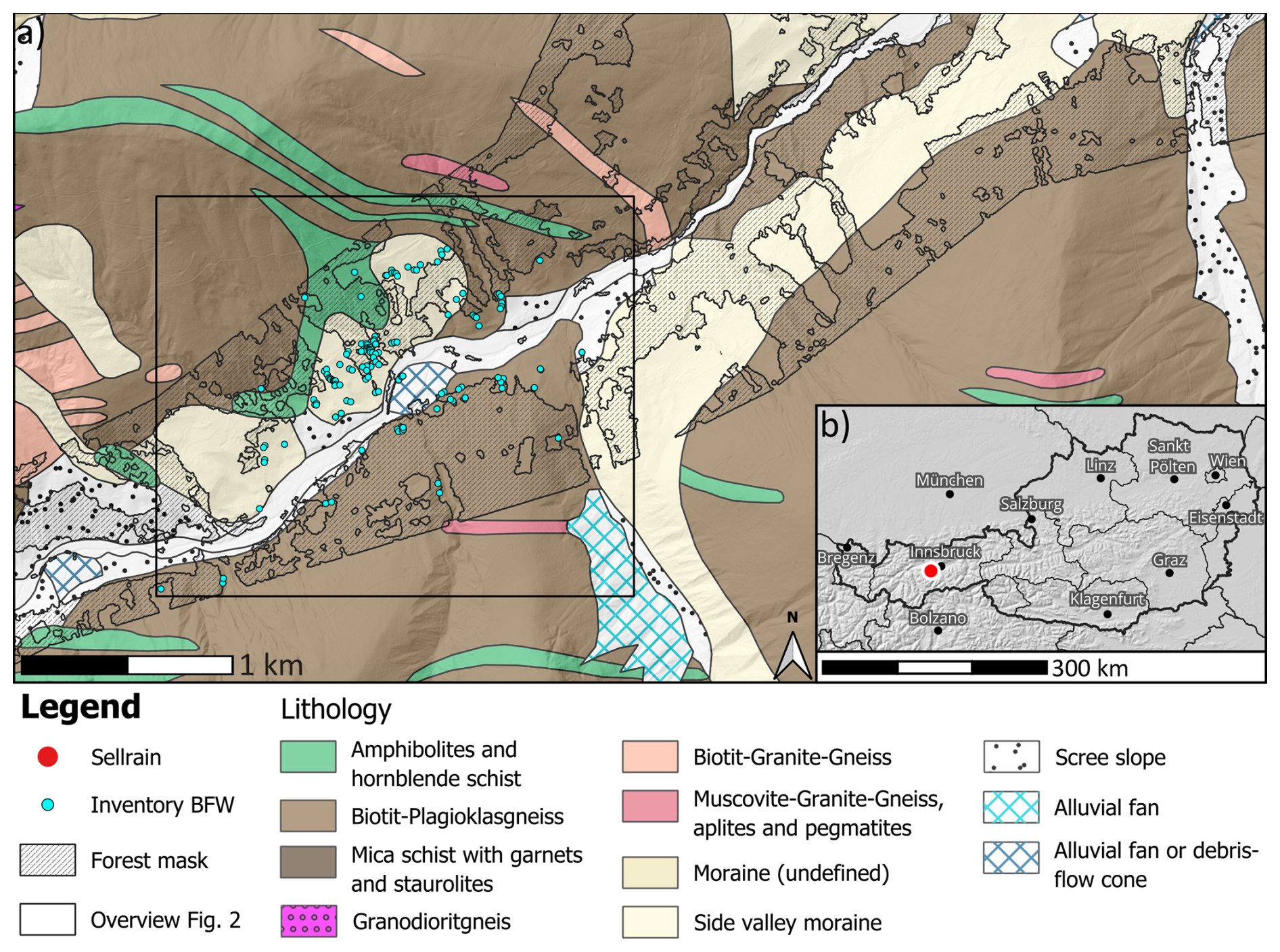
Figure 1 Overview of the study area near the village of Sellrain, Austria. (a) shows the full study area with the lithological map (GeoSphere Austria, 2021), the 2017 ALS DTM hillshade (provided by the federal state of Tyrol), the forest mask, the BFW landslide inventory and the extent of the focus area for model training (cf. Fig. 2); (b) shows the location of Sellrain in Austria (red dot), with a hillshade derived from the EU-DEM (Copernicus Land Monitoring Service, 2016) and administrative boundaries taken from the NUTS dataset (Eurostat).

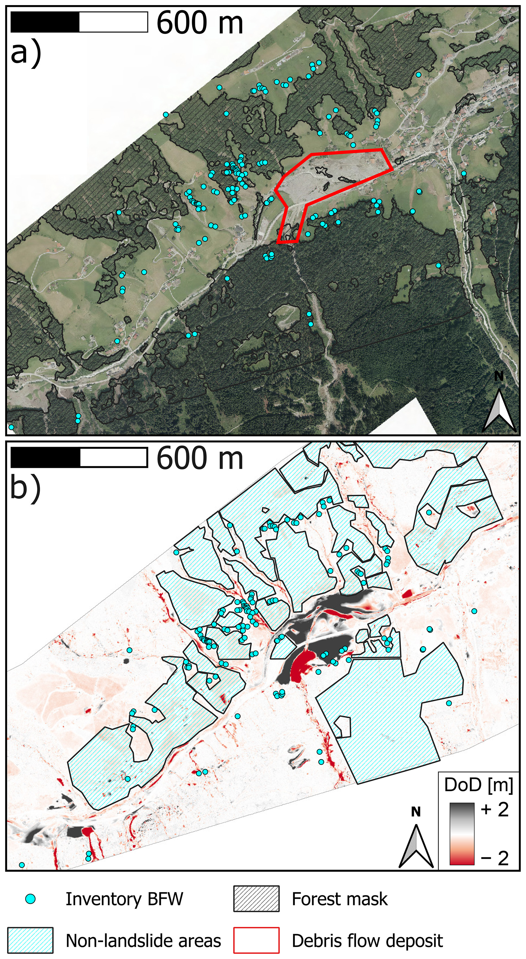
Figure 2 The focus area of the training datasets with (a) the post-event orthophoto (provided by the federal state of Tyrol), the BFW inventory, the forest mask and the location of the debris flood deposit; (b) the DoD of the 2013 and 2017 ALS DTMs (data provided by the federal state of Tyrol), the non-landslide areas and the BFW inventory.

The investigations in this study focused on an area of 8 km², limited by the coverage of the DoD, around the village Sellrain. The DoD covers the lower elevation sections of the valley with elevations ranging between 780 and 1410 m a.s.l. The valley is incised by the Melach river flowing from southeast to northwest. The study area also includes a section of the Seigesbach catchment (stretching in south-southeast to north-northwest direction) which terminates in the Melach river just west of the village Sellrain. The village Sellrain is located on the alluvial fan of this torrent. The study area is further characterised by steep slopes with an average slope angle of 28°. With regards to the geology, the study area is part of the Ötztal-Stubai crystalline complex, with formations mainly consisting of gneisses (e.g., “Schiefergneis”) and side moraine deposits (Moser, 2011) (Fig. 1a). An analysis of the forest canopy cover mask created in this study shows that 46 % of the study area is covered by forest (a high tree density), with the remaining landcover consisting of grassland (used mainly as meadows) and built-up areas. The predominant forest ecosystem is montane silicate spruce forest, consisting mainly of Norway spruce (Picea abies) with an admixture of European larch (Larix decidua) and of single trees or patches of grey alder (Alnus incana) and birch (Betula pendula) (Land Tirol, 2014). In addition, an analysis with the forest mask also showed that the slopes are generally steeper within the forest with an average slope angle of 33° against an average of 23° outside the forest mask.

2.2 Rainfall event characteristics

The investigated event occurred 7–8 June 2015. In the night of the 7th, 100–150 mm rain fell within a span of 12 h (Lagger, 2015). According to a reanalysis of weather radar data (GeoSphere Austria, 2015), the event was very short and intense (Fig. 3). Rainfall started at 19:00 UTC on the 7th with 7 mm h⁻¹. The peak occurred at 20:00 UTC with almost 60 mm h⁻¹. After 22:00 UTC the rainfall had already fallen below 5 mm h⁻¹ and below 1 mm h⁻¹ at 02:00 UTC. It should also be noted that May was wetter than average (Jenner, 2015) and it can thus be expected that the antecedent moisture content also played a role in the initiation of the landslides.

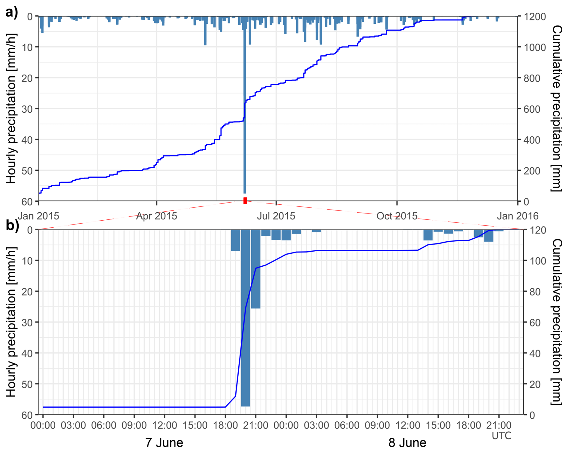
Figure 3 Reanalysis of the rainfall event with radar data from the INCA dataset (GeoSphere Austria, 2015). (a) Hourly precipitation data for the entire year 2015. (b) Hourly precipitation data for 7 and 8 June 2015.

2.3 Landslide mapping in the field

The landslide inventory that was constructed by the BFW found 136 landslides related to the event (Figs. 1 and 2). This inventory includes a point-based dataset that was collected under standard conditions for hazard event documentation in the field and through visual inspection of an orthophoto taken on 10 June 2015 (Fig. 2a). The area of interest for the inventory was the area around the village of Sellrain and the area along the Seigesbach creek. A first analysis of the inventory with a canopy cover mask (Sect. 3.2; Figs. 1 and 2) shows that only 10 landslides are located inside the forest mask. Therefore, an important step of this study was to first detect additional landslides within the forests, as the BFW inventory may systematically underestimate them.

3 Materials and methods

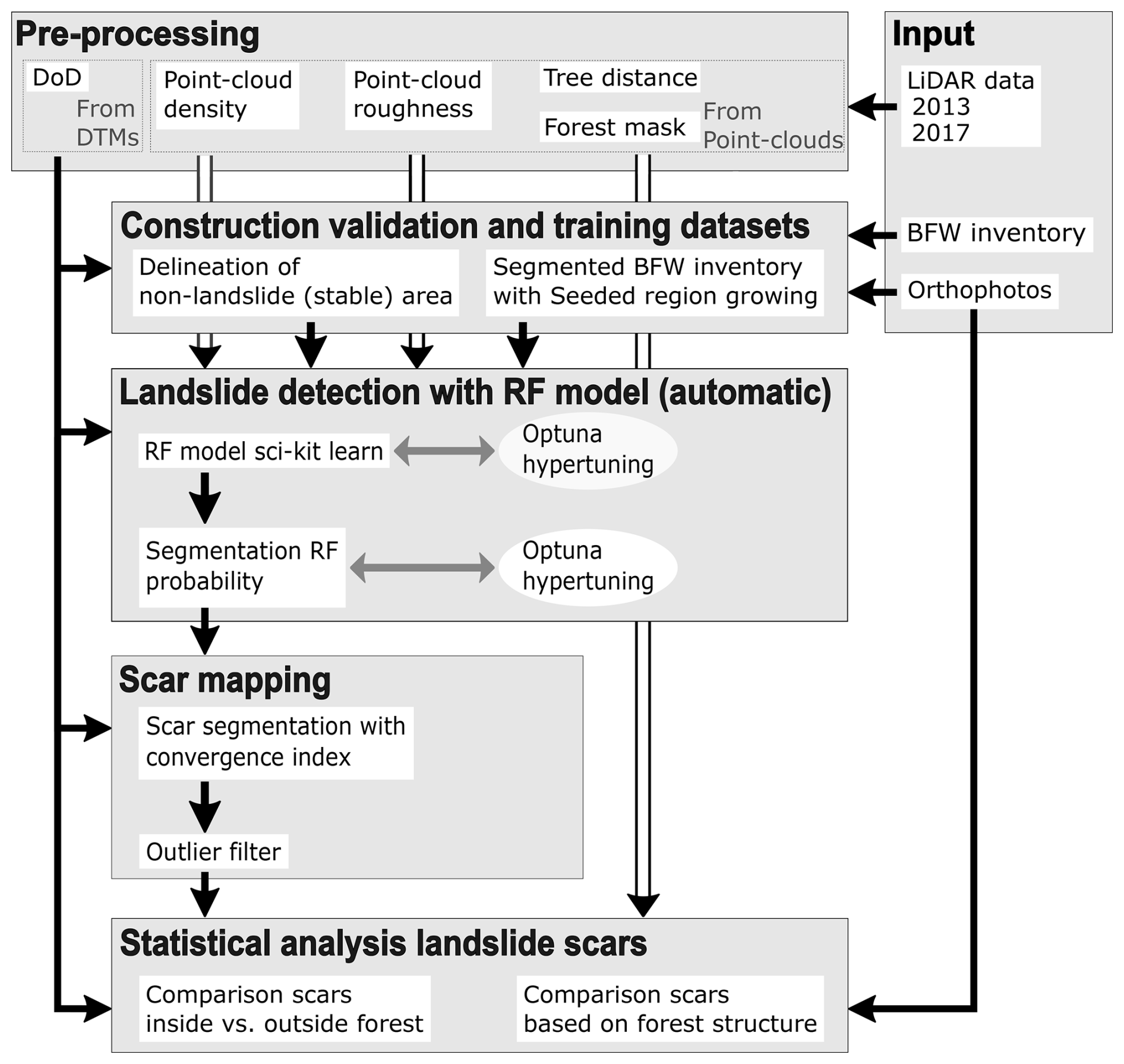
An overview of the full workflow used in this study is given in Fig. 4. The first main step of the workflow consisted of collecting, pre-processing and creating all the datasets that would be used in further analyses of the landslides, including the construction of a forest canopy cover mask. Since the existing landslide inventory from the BFW is a point-based inventory, the second main step of the workflow was to develop a polygon-based inventory from the existing points using a seeded region growing algorithm (Adams and Bischof, 1994; Bechtel et al., 2008; Conrad et al., 2015) (see Sect. 3.2). The second main step also consisted of delineating areas without landslide signs in the DoD and orthophoto data, further referred to as non-landslide areas. Both datasets were used for validation and training in later steps of the workflow. The third main step of the workflow was to detect additional landslides within the forest, since the BFW inventory only contained limited samples within that category. For this, a random forest (RF) model was trained on the polygon-based, segmented BFW inventory and the non-landslide areas using DoD data derived from two ALS acquisitions acquired before and after the 2015 event. After the model was trained, a filtering and segmentation algorithm was used on the probability output of the RF model to construct the landslide detection map. The fourth main step in the workflow consisted of mapping the scars (the depletion zone) within the detected landslide areas. The final main step in the workflow was then to analyse the morphological and topographic profile characteristics of the mapped scars and the relationship of these characteristics with the location of the scars relative to the forest canopy cover mask and surrounding trees. For this the scars were classified into located within the forests (in this study defined by a share of the canopy cover mask ≥90 %) and located outside the forest (in this study defined by a share of the canopy cover mask =0 %). Additionally, the scars were also analysed based on the closest tree distance from each scar cell and the average number of trees within a 10 m radius of the scar cells. To rule out effects of past forest cover changes at the locations of the mapped scars, the final analysis only included scars at locations where landcover had not changed in the 20 years prior to the 2015 storm event. The landcover change was analysed at each of the scar locations with a visual inspection of historic aerial imagery.

Figure 4 General workflow of the study.

3.1 Available datasets and pre-processing

Several datasets were used for the analysis of the landslide scars in the Sellrain valley, of which the two ALS acquisitions from 2013 and 2017 were the most important. These datasets were provided by Federal State of Tyrol as classified point-cloud and their corresponding 0.5 m resolution DTMs. Details on the accuracy of these datasets are given in Table 1.

Table 1 Accuracy and point density information of the two (2013 and 2017) ALS acquisitions. The point density was determined from a representative subsection of the point-clouds.

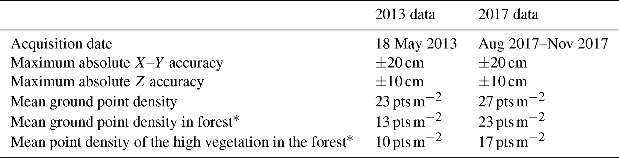
^* The points in the forest were extracted with the forest mask created in this study.

The ALS datasets were used to construct a DoD from the provided DTMs. In addition to this, the 2013 ALS dataset was also used to construct a binary forest canopy cover mask. The LIS Pro 3D grid-based forestry toolchain from LIS Pro 3D v2024.03 (LIS Pro 3D, 2025) was used to extract single tree positions and a binary canopy cover map from a canopy height model constructed with the 2013 point-cloud data (Eysn et al., 2012). The binary canopy cover mask was created by extracting all trees with a height of at least 2 m from the canopy height model and thresholding the canopy cover of these trees at 30 %. The extracted single tree positions were also used to construct a tree distance map and a tree neighbour count map, where each cell of the map was assigned the closest distance to a tree and the number of trees within a 10 m radius. The 2013 and 2017 ALS point-clouds were also used to derive the density and elevation roughness, calculated from the standard deviation of the elevation values, of the ground points within the grid cells of the DTMs.

In addition to this, there was also a 0.1 m resolution orthophoto provided by the Federal State of Tyrol. This orthophoto was acquired using an airplane on 10 June 2015, only a few days after the investigated event. In this study, the dataset was used for validation of the landslides detected by the RF model. Besides the 2015 orthophoto, the study also made use of further historic orthophotos starting from 1988 until 2015 to analyse landcover changes in the study area (Land Tirol, 2025). Lastly, for filtering bank erosion and landslides located near roads, the map of the stream network in Tyrol (Land Tirol, 2023) was used to construct a stream mask and data from the road network (ÖVDAT, 2022) was used for a road mask, both masks were constructed by applying a 15 m buffer on the datasets.

3.2 Segmentation of BFW landslide inventory and construction non-landslide area

To construct a polygon-based inventory from the existing point-based BFW inventory, a seeded region growing algorithm from SAGA GIS (v9.7.2) (Adams and Bischof, 1994; Bechtel et al., 2008; Conrad et al., 2015) was used on the original dataset. The input features consisted of a downscaled DoD (0.1 m resolution) and the after-event orthophoto. The delineation of the scars from the seeded region growing algorithm was checked against the orthophoto and DoD, including its slope, hillshade and topographic openness at 5 and 10 m. These derivatives are often used in landslide mapping as they can clearly delineate the edges of landslide scars (Petschko et al., 2016; Razak et al., 2011).

It was unknown how many additional landslides occurred within the 2013 to 2017 timespan. This meant that use of the full area in the training dataset for training of the RF landslide detection model could include many landslides falsely classified as stable or unchanged areas within the training dataset. For this reason, it was decided to also delineate areas where no landslides were present in the DoD dataset and only use the segmented scars of the BFW inventory and this “non-landslide” area for the training of the landslide detection model. The non-landslide area was delineated after visual inspection of the orthophoto and DoD, including DoD derivatives such as the slope, hillshade and topographic positive openness.

3.3 Landslide detection with RF model

For the detection of additional landslides, an RF model was trained on the segmented BFW inventory and the non-landslide area. The framework for the RF model was taken from the scikit-learn Python library (v1.5.1) (Breiman, 2001; Pedregosa et al., 2011). The input of the RF model consisted of the DoD and several DoD uncertainty proxy datasets. The change estimation values from a DoD dataset come with uncertainties that result from the simplification of the original point-cloud datasets, which occurs in the construction of the underlying DTM datasets. These uncertainties can be approximated with the point density of the point-cloud and the surface roughness of the terrain (Li et al., 2024). To account for the DoD uncertainty in the landslide detection model, it was decided to use the point-density and elevation roughness of both years as additional input in the RF model. The final input of the RF model thus consisted of the DoD and four uncertainty proxy layers.

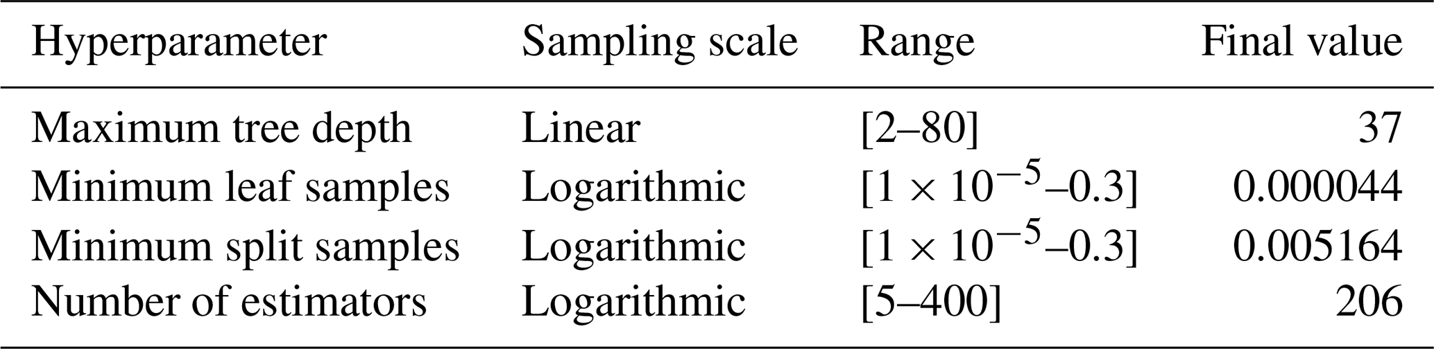
To hypertune the RF model (i.e., to optimize the hyperparameters of the model, such as the maximum tree depth of the random forest), a set-up was created in Python using the Optuna library (v4.0.0). The Optuna library provides a framework for optimizing the search of the optimal hyperparameter combination within a large hyperparameter space (Akiba et al., 2019). The value ranges used for the hyperparameter tuning are given in Table A1 in the Appendix. To optimally search the hyperparameter space, the Optuna framework fits an optimization function from the hyperparameters of previous runs and a chosen model performance metric. In this study it was decided to use the area under the curve (AUC) metric and the Jaccard index derived with three cross-validation folds for the hyperparameter optimization. The training dataset was split into three subsets for hypertuning (20 %), training (48 %) and testing (32 %) of the model. The final hyperparameter set-up was based on the model run with the highest AUC value, the parameter values of this set-up are given in Table A1 in the Appendix.

After the RF model was hypertuned and trained, the probability output from the RF model was segmented with a separate segmentation workflow, since the classification by the RF model led to large overestimation of landslide locations. An overview of the full workflow is given in Fig. A1 in the Appendix. The first step of this segmentation workflow was a segmentation and filtering of the RF probability output. The filtered probability output was then used to extract seed locations and perform seeded region growing with the seed generation and seeded region growing tools from SAGA GIS (v9.7.2). The input for the seeded region growing consisted of the RF probability, the DoD, and the average RF probability within a specific window size. The region growing resulted in several smaller segments with similar probability values. In a next step, these segments were clumped together with the r.clump algorithm from GRASS GIS (v7.8) (GRASS Development Team, 2024) based on their average probability. These clumped segments were then filtered based on their size and average probability.

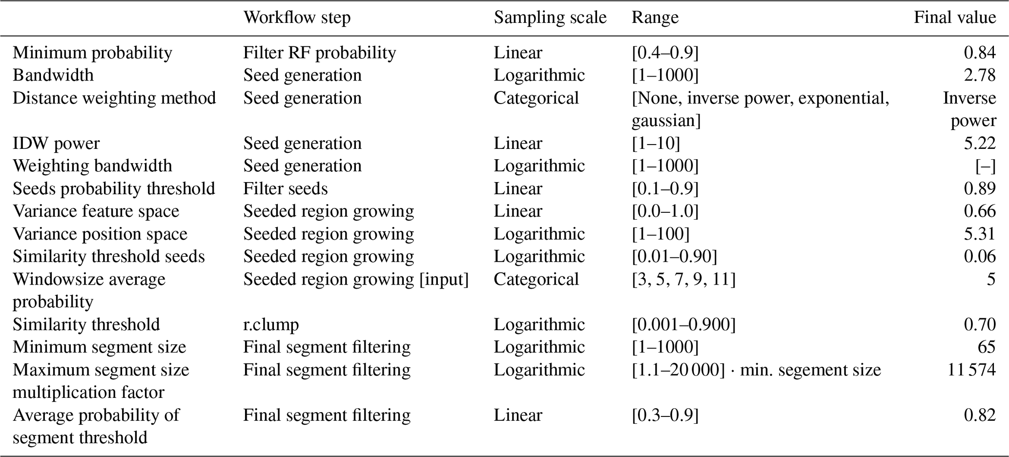
Since the full workflow required many parameters, it was decided to also use the Optuna optimization workflow for their optimization. The full list of parameters and their final calibration values are given in Table A2 in the Appendix. The optimization in Optuna for the segmentation workflow was based on the distance to the perfect classification (D2PC) and Jaccard index. Since the filtering of false positives was deemed more important than a detection of all the occurred landslides, the decision of the best parameter set-up was based on the Jaccard index.

3.4 Mapping of additional scars from RF detection

The final step of the RF inventory construction was mapping the landslide scars within the detected landslide area by the RF model. For this, the convergence index from SAGA GIS (v9.7.2) (Conrad et al., 2015; Koethe and Lehmeier, unpublished, 1996) was used to detect sink and peak areas within the DoD dataset. Since the scars of the landslides are represented as distinct sinks within the DoD data, a negative threshold on the convergence index was used to map the landslide scar areas. A visual inspection of the convergence index at different threshold levels showed that a threshold of −30 % was best at separating the scar areas from secondary erosion zones, such as gully erosion, while also preserving the size of the landslide scar. After the best threshold was selected, the convergence index was segmented and each of the segments overlapping with the landslide detection output were validated. Only the segments showing landslides signs in the DoD or orthophoto were kept in the final inventory. Outliers of underestimated scar segments, where the convergence index only captured a steep pit within the landslide scar, were filtered out using the minimum scar size from the BFW inventory.

3.5 Morphological and topographic profile analyses of the scars and their forest cover

The main goal in the analysis of the RF scars was to investigate the differences between landslides within the forest and those located outside the forest. To achieve this, the scars first had to be classified according to their forest canopy cover. If a scar segment was covered for 90 % or more by the constructed canopy cover mask, the scar was classified as located within the forest. If the scar did not have any cover from the constructed canopy cover mask (cover=0 %), it was classified as located outside the forest. To create a better distinction between landslides within and outside of the forest, landslides with partial cover <90 % were excluded from this binary analysis. Additionally, the historic aerial imagery from 1988 to 2015 was also used to filter-out any landslides that were situated at locations where the forest cover had changed in the 20 years leading up to the storm event of 2015, e.g., at locations of afforestation or deforestation. In this way, it was ensured that the statistical analysis of the landslides was not obscured by, for example, landslides outside the forest at locations of deforestation, as they might still be affected by the effects from past forest cover. To analyse the relationship between the forest structure and the characteristics of the landslides, additional analyses were also performed based on a tree distance map and a map of the tree count within a 10 m radius from each cell. These maps were used to extract, for each of the scars, the minimum of the closest tree distances from each scar cell (i.e., the closest tree distance) and the average number of trees located within a 10 m radius, derived from the tree counts of the individual scar cells. The forest structure analysis included the landslides with partial forest cover (<90 %).

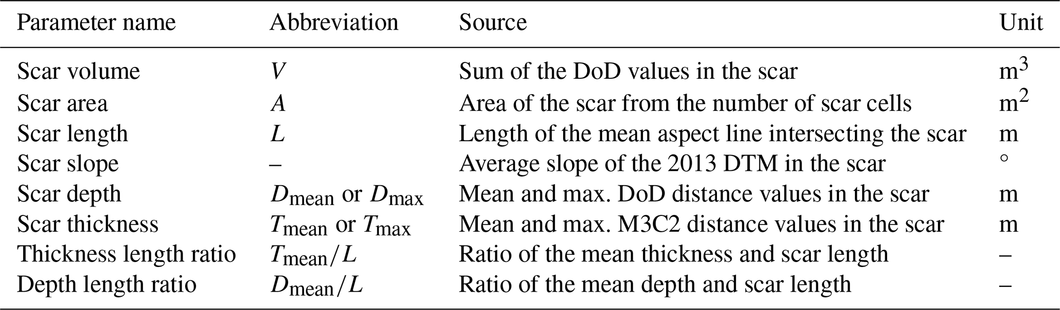
Both the forest classification and the parameters with information on the trees surrounding the scars were then used to investigate their relationships with the morphological characteristics of the scars. The analysed morphological scar parameters were the scar area (A), scar depth (D), scar thickness (T), scar volume (V), scar length (L), scar slope and ratios of the scar length with its mean depth ($D_{\text{mean}}/L$) and thickness ($T_{\text{mean}}/L$). An overview of these parameters, their abbreviations and sources is given in Table 2. To extract the landslide thickness, which in this study is defined as the distance from the original topography to the landslide slip surface in the slope normal direction, an additional topographic distance map was constructed from the two DTMs with the M3C2 method from CloudCompare (v2.14) (Lague et al., 2013). Additionally, a line along the aspect direction of the slopes was also used to extract the scar length. The length parameter was used to derive the ratios of the scar depth and thickness with its length. These are all parameters that are often used in the analysis of landslides (Rickli and Graf, 2009; Schaller et al., 2025; Zieher et al., 2016).

Table 2 Overview of the morphological parameters, their abbreviations and the source of their construction.

Besides a visual inspection of the relationship of these parameters with the forest parameters using boxplots and scatter plots, the statistical relevance of their relationship was also investigated with a Wilcoxon-Withney U test and Welch's t-test for the binary classification of the scars according to their forest classification. The relationships with the distance to the closest tree parameter and the parameter describing the number of trees in the vicinity of the scar were analysed with Welch's analysis of variance (ANOVA) test. The Mann-Withney U test and Welch's t-test set-ups were taken from standard set-ups in the scipy (v1.15.1) Python library (Virtanen et al., 2020). The Welch's ANOVA test was taken from the statsmodel (v0.14.4) Python library (Seabold and Perktold, 2010; Welch, 1951).

The topographic profiles of the landslides were analysed by extracting the thickness of the landslides along their profile lines. To enable a comparison between the different scars, two profile lines with fixed length were drawn through the centroids of the scars along the average aspect direction within the scar and perpendicular to this aspect direction. To compare the thickness profiles from the scars inside and outside of forests, the median and the inter-quartile range (IQR) of the thickness was calculated for each classification along the extracted profiles. Differences between the median thickness profiles were quantified by calculating the root mean squared deviation (RMSD) of the median profiles along segments of the profiles.

4 Results

4.1 Landslide detection based on the RF model and scar extraction

The probability output from the RF detection model is shown for two example areas in Fig. 5i and j. The model performance of the final RF model has a Jaccard index of 0.049 and an AUC value of 0.94, tested with the hypertuning dataset. The ROC-curves of the random forest model on the esting and training datasets are given in Fig. 6a. Using the testing dataset and with a filter of the probability output on the threshold with the best D2PC value of 0.19, the TPR (true positive rate) and FPR (false positive rate) are 85 % and 13 %, respectively. Note that these performance metrics are calculated on a pixel-basis.

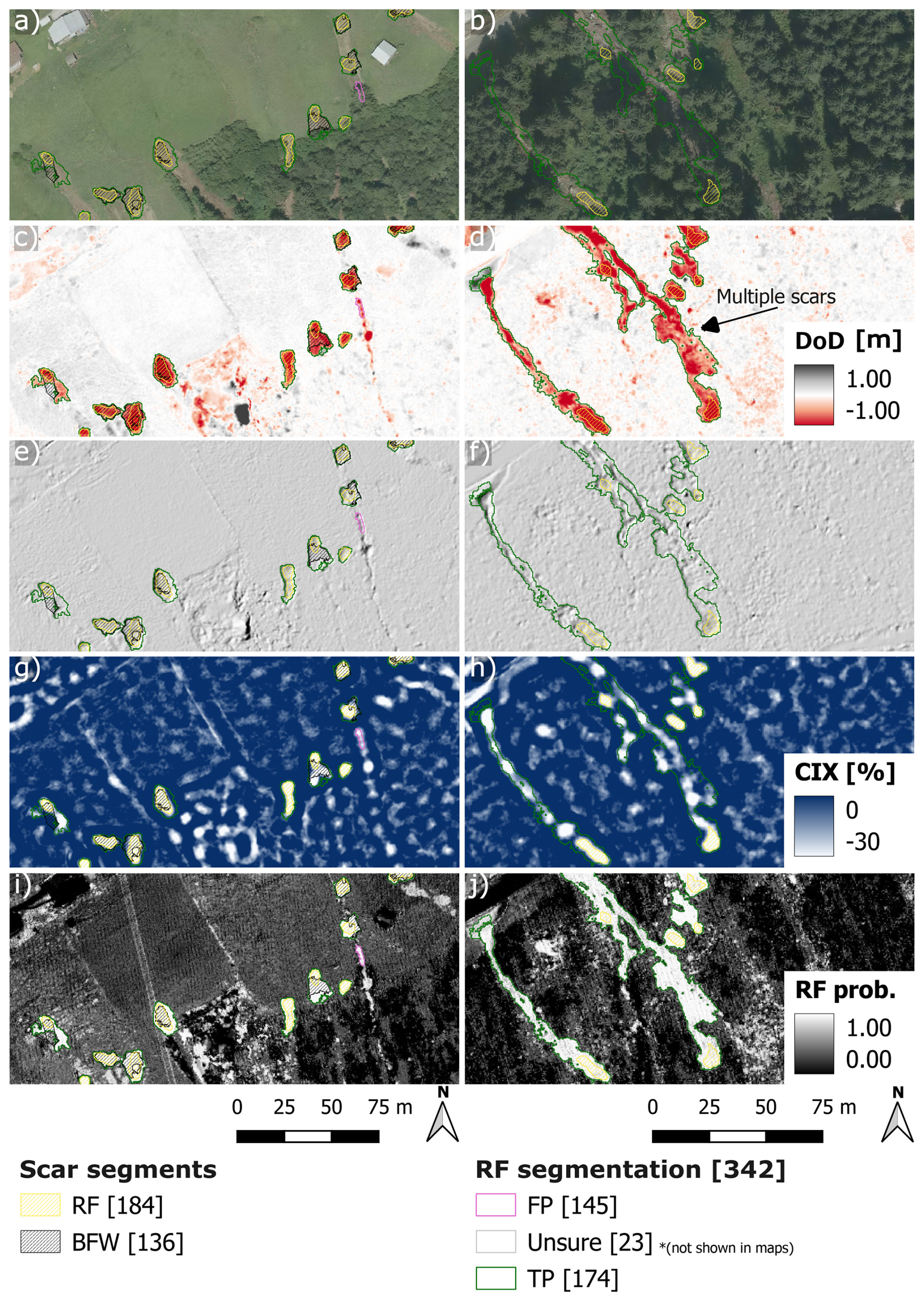
Figure 5 Output of the RF segmentation and subsequent scar mapping compared with the original BFW inventory for two example areas, shown on the post-event orthophoto (a, b), the DoD (c, d), a hillshade of the DoD (e, f) (all three base layers provided by the federal state of Tyrol), the convergence index (CIX) used in the scar mapping (g, h) and the probability output of the RF model (i, j).

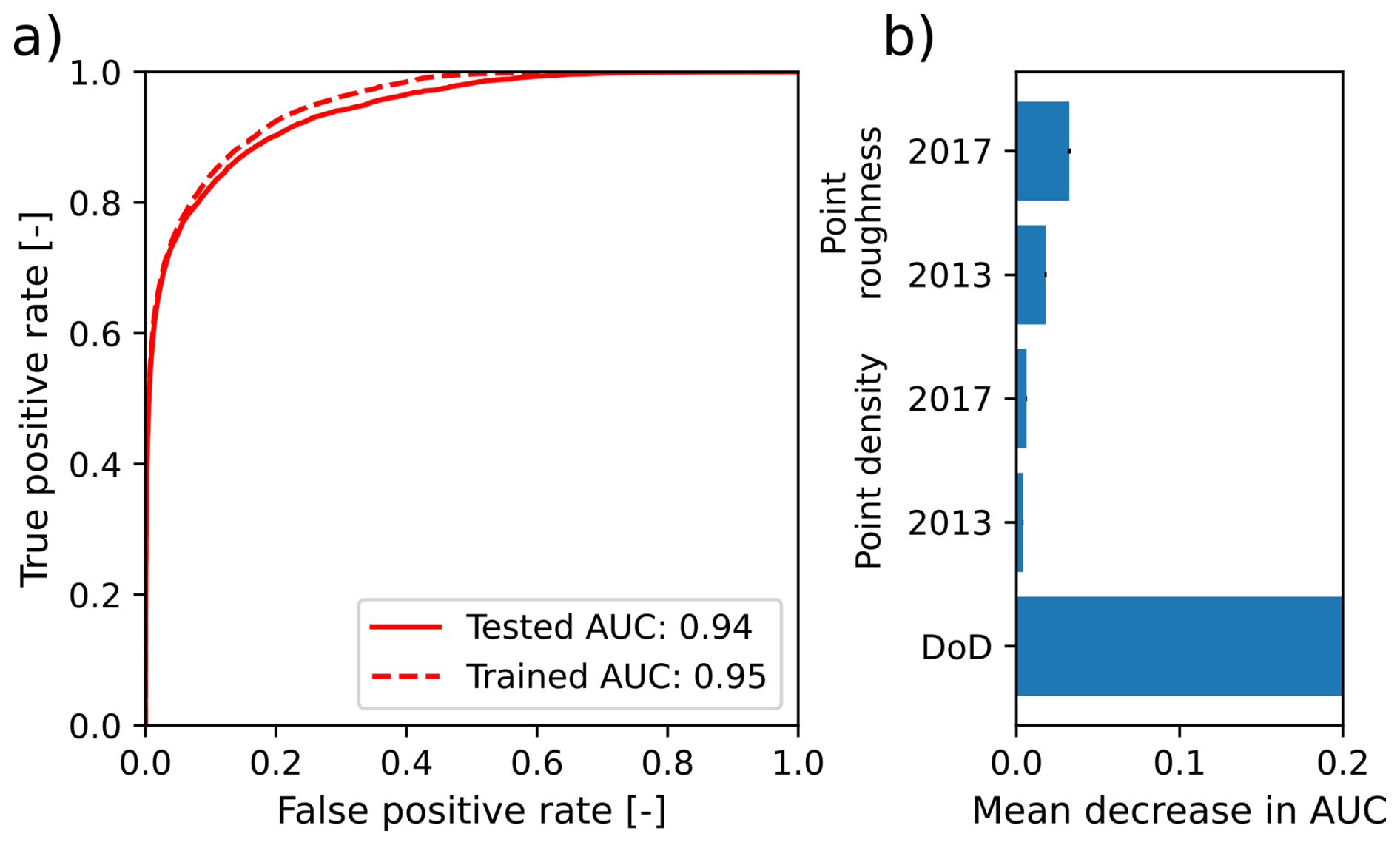
Figure 6 (a) ROC curve of the trained RF detection model and (b) feature importance of the input features, measured as mean decrease in AUC value.

An analysis of the feature importance of the trained random forest model is given in Fig. 6b. The feature importance was assessed with the scikit-learn (v1.5.1) Python library (Breiman, 2001; Pedregosa et al., 2011) through permutation of the individual features of the model input and assessing the impact of this permutation on the model performance, in this study the AUC score. The results show, as expected, that the DoD has the largest impact on the model performance with an average drop in AUC of 0.20. After the DoD, the roughness of the 2017 data has the largest impact on the model performance, followed by the roughness of the 2013 data. Respectively, they result in an average a drop in AUC of 0.03 and 0.02 after their permutations. The point-density layers of 2017 and 2013 see an average drop of 0.006 and 0.004, respectively. It should be noted with this analysis that the point-density and roughness datasets are related to each other and a univariate analysis results in biased statistics, which could lead to lower values of feature importance for these layers.

Since the classification results of the RF model resulted in a high degree of overestimation, also in terms of number of landslides, it was decided to apply an additional filtering and segmentation algorithm to the probability output of the RF model. The results from this are given in Fig. 5. The trained algorithm has a Jaccard score of 0.52 and a D2PC value of 0.26. The false positive rate is only 0.18 %, with a TPR of 73.8 %. Note that these performance metrics are also calculated on a pixel-basis. A manual check of each of the segmented polygons resulted in 54 % true positives on an object-basis. 45 % of the polygons were deemed false positives. The results from the final output of the landslide detection algorithm are also shown in Fig. 5.

After mapping the scars in the detected landslide areas with the convergence index, 184 landslides were found of which 51 are covered for more than 90 % by the canopy cover mask. 65 landslides intersect with a landslide in the BFW inventory. An analysis of the BFW landslides that were not detected by the RF inventory showed that a large number was either located on the debris flood deposit or too shallow to leave signs in the DoD data. Thus, the RF model found 119 additional landslides. A summary on the landslide characteristics from both the RF and BFW inventories is given in Table 3. The plots in Fig. 7 show the relationships of the landslide scar areas with their volume (Fig. 7b) and mean depth (Fig. 7c), for the original BFW and new RF inventories. Both inventories mainly consist of shallow landslides, with mean depths below 2 m for most of the scars. In addition, the relationship of the landslide volume and area in the RF inventory is very linear, while for the BFW inventory the relationship is more spread with a larger range of landslide depths for different scar sizes.

Table 3 Summary statistics of the RF and BFW inventories with mean scar areas, mean DoD values and mean scar volume, calculated with the scars remaining after the outlier filter. The statistics are calculated separately for the full inventory, the landslides inside the forest, the landslides outside the forest and those with partial forest cover. The table also provides the scar counts remaining after each filtering step.

¹ Calculated with the “No outliers” subset. ² Land-cover change (LCC). The scars with “No LCC” were only part of the RF inventory.

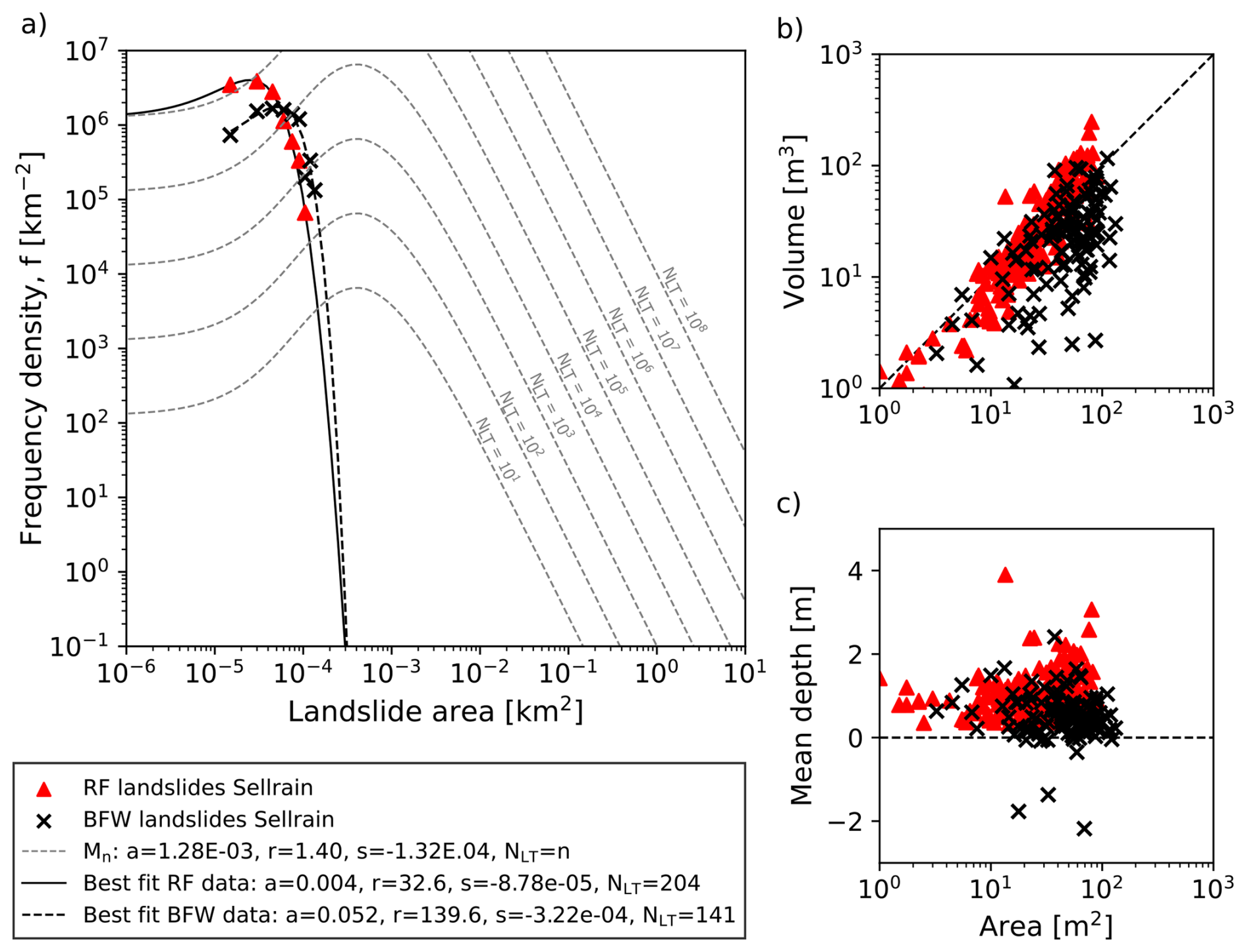
Figure 7 Frequency density distributions of the BFW (in black) and RF (in red) scar areas (a). No outlier filter was applied to the data. The fitted curves are fitted according to the Malamud distribution, of which the standard distributions are also given as grey dotted lines for different landslide inventory sizes. The plots on the right show the relationship of the scar areas with their volume (b) and with their mean depth (c).

The plot in Fig. 7a shows the frequency density distribution for the scar areas of the RF and segmented BFW inventories. The plot shows that, as proposed in Malamud et al. (2004), the landslides follow a power-law distribution with a drop in frequency for the smallest scar areas. What should be noted is that the distributions of both the RF and BFW inventories are quite different from the Malamud distributions with a shift to lower area sizes with a factor 20. However, it should be noted that the inventories analysed in Malamud et al. (2004) consider the full process area, while the constructed inventory in this study only considers the scar area.

It is clear from these figures that both datasets contain outliers. The distributions in Fig. 7 and the statistics in Table 3 also indicate that some of the landslides in the RF inventory have a very small scar area <3 m². Additionally, the BFW inventory also contains several landslides located on the debris flood deposit, which results in negative mean depth and volume estimates from the DoD data. These landslides were filtered out with the outlier filter. They are not considered in the remaining analyses.

4.2 Morphological and topographic profile analysis of the RF scars in forests and outside of forests

The analyses of the landslide characteristics in relation to their forest cover and the forest structure parameters were performed on a subset of the RF landslides that did not overlap with locations of significant land-cover changes. This subset consisted of 110 landslides, of which 39 are classified as in the forest and 60 are classified as outside the forest (Table 3).

Comparisons between the landslides inside and outside the forest, according to the binary forest cover classification, of the morphological parameter distributions of the scars in this subset are given in Fig. 8, with a statistical summary given in Table 4. The comparison shows that there is a difference in all investigated parameters except for the area and volume estimations of the scars. The statistical relevance of these differences was also tested with Mann Withney U tests and Welch's t-tests (Table 4). The Mann Withney U tests and Welch's t-tests showed that, besides the distributions of the area and volume parameters, all distributions of the investigated parameters show statistically relevant differences when they are split by their forest cover classification, with p-values<0.02.

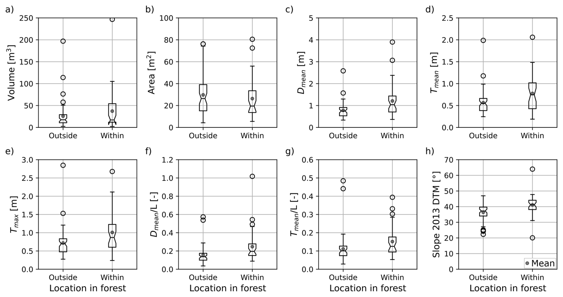
Figure 8 Distributions of the morphological scar parameters in the RF inventory visualized as boxplots with a grouping according to the landslide forest cover (within or outside the forest). The plotted parameters are the (a) scar volume, (b) scar area, (c) the mean scar depth, (d) the mean scar thickness, (e) the maximum scar thickness, (f) the mean depth/length ratio, (g) the mean thickness/length ratio and (h) the average slope in the 2013 DTM.

Table 4 Statistical summary (average, standard deviation and interquartile range (IQR) values) of the morphological parameter distributions for the scars inside and outside the forest with the statistical significance of the differences between the scars inside and outside the forest as calculated with the Mann-Withney U test and Welch's t-test.

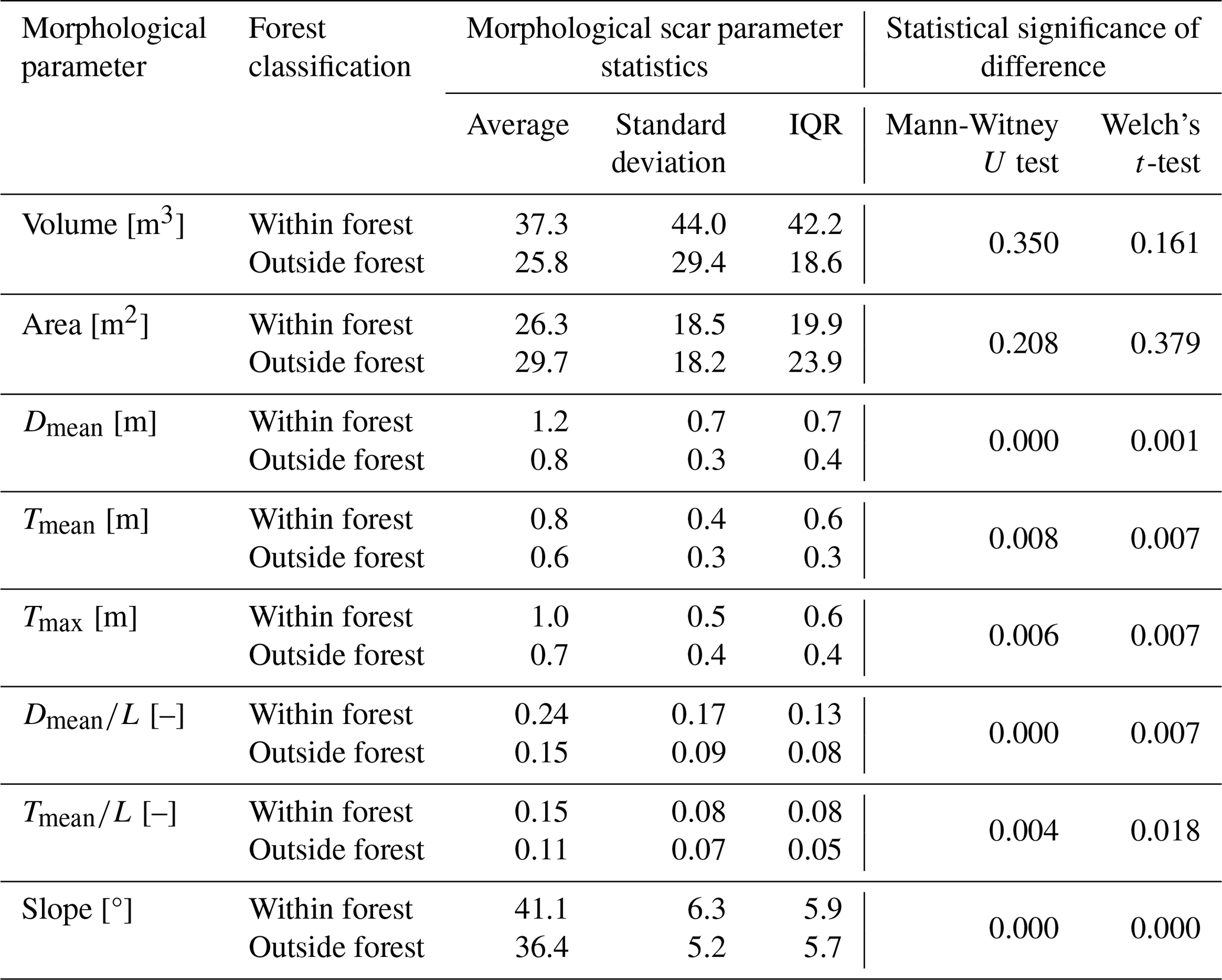
The mean depth (D_mean) distributions show that there is a difference between the mean depth values of the scars inside the forests and those outside the forest, with respective average “mean depth” values of 1.2 and 0.8 m. The standard deviation and IQR values for each of the morphological parameters are given in Table 4. The difference in mean depth is also reflected in the $D_{\text{mean}}/L$ ratios of the scars, with a larger average ratio for the scars inside the forest of 0.24 against an average ratio of 0.15 for the scars outside the forest. The distributions of the mean thickness (T_mean) also show a similar difference. The T_mean values are on average larger for the scars inside the forest, with respective average values of 0.8 m inside and 0.6 m outside the forest. Similarly, the maximum thickness values (T_max) are on average also larger in the forest, with an average of 1.0 against 0.7 m, respectively inside and outside the forest. The $T_{\text{mean}}/L$ ratios also reflect this difference with respective average values of 0.15 and 0.11 inside and outside the forest. Lastly, the distributions of the mean slope from the pre-event DTM of the scars show that the pre-failure slope is on average steeper for the scars inside the forest, with an average of 41.3° against an average of 36.4° for the scars outside the forest.

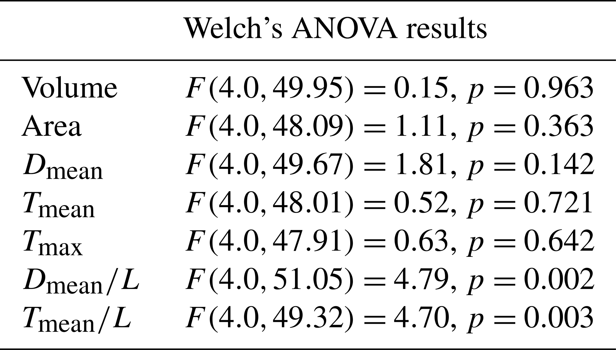
Figure 9 shows the relationship of the closest tree distance of the scars with the different morphological parameters. The plots show that there is a relationship between the closest tree distance and all of the morphological parameters except for the scar area. Thus, similarly to the analysis with the binary forest mask, the landslides located closer to trees also show greater depths and thicknesses, higher thickness- and depth-to-length ratios and steeper pre-failure slopes. Additionally, the analysis with the forest structure parameters also shows significantly larger scar volumes for landslides located closer to trees. An ANOVA on the formed groups from the plots in Fig. 9 shows that except for the area parameters, the differences between the groups of all parameters is statistically significant with p-values from the ANOVA all falling below 0.05 (Table 5).

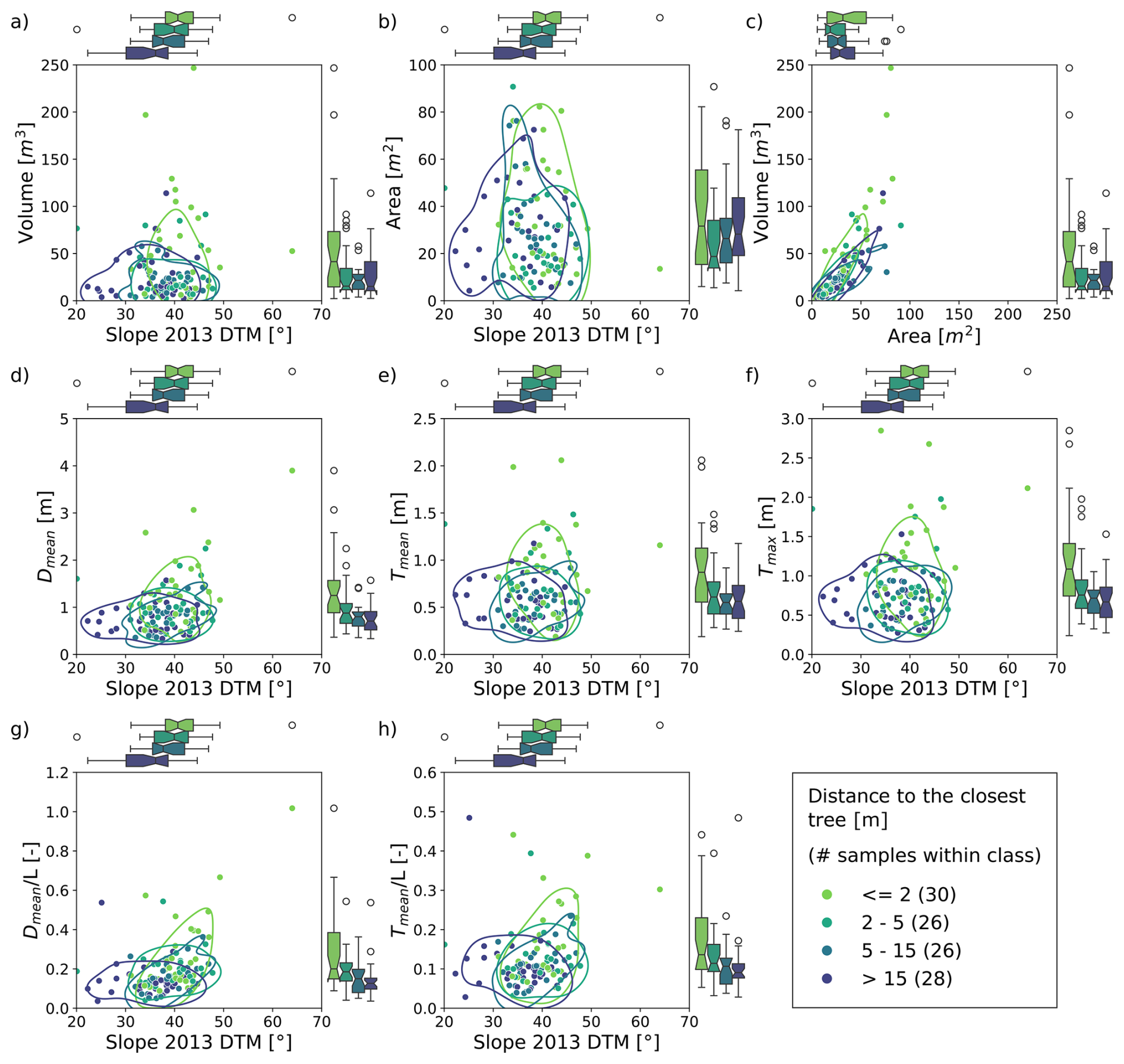
Figure 9 Analysis of the relationship between scar morphology and the average pre-failure slope of the scars (from the 2013 DTM data), coloured by the distance to the closest tree of each scar. The contour boundaries show the 75th percentile boundary of the binned tree distance subsets. The plotted morphological parameters are (a) the scar volume, (b) the scar area, (c) the scar volume against the scar area (instead of the 2013 DTM slope), (d) the mean depth, (e) the mean thickness, (f) the maximum thickness, (g) the mean depth to length ratio and (h) the mean thickness to length ratio.

Table 5 ANOVA results on the grouped data and parameters from Fig. 9.

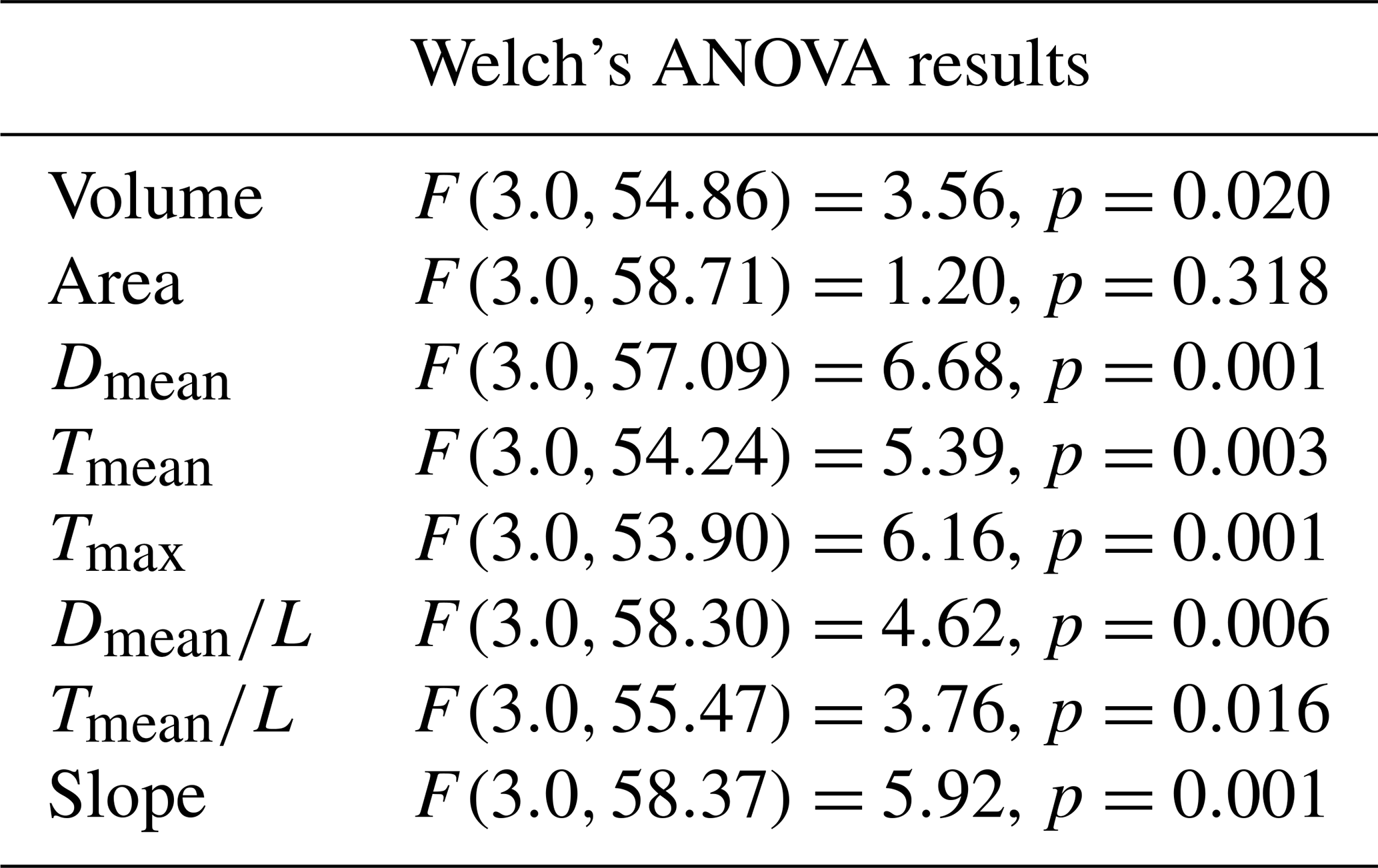
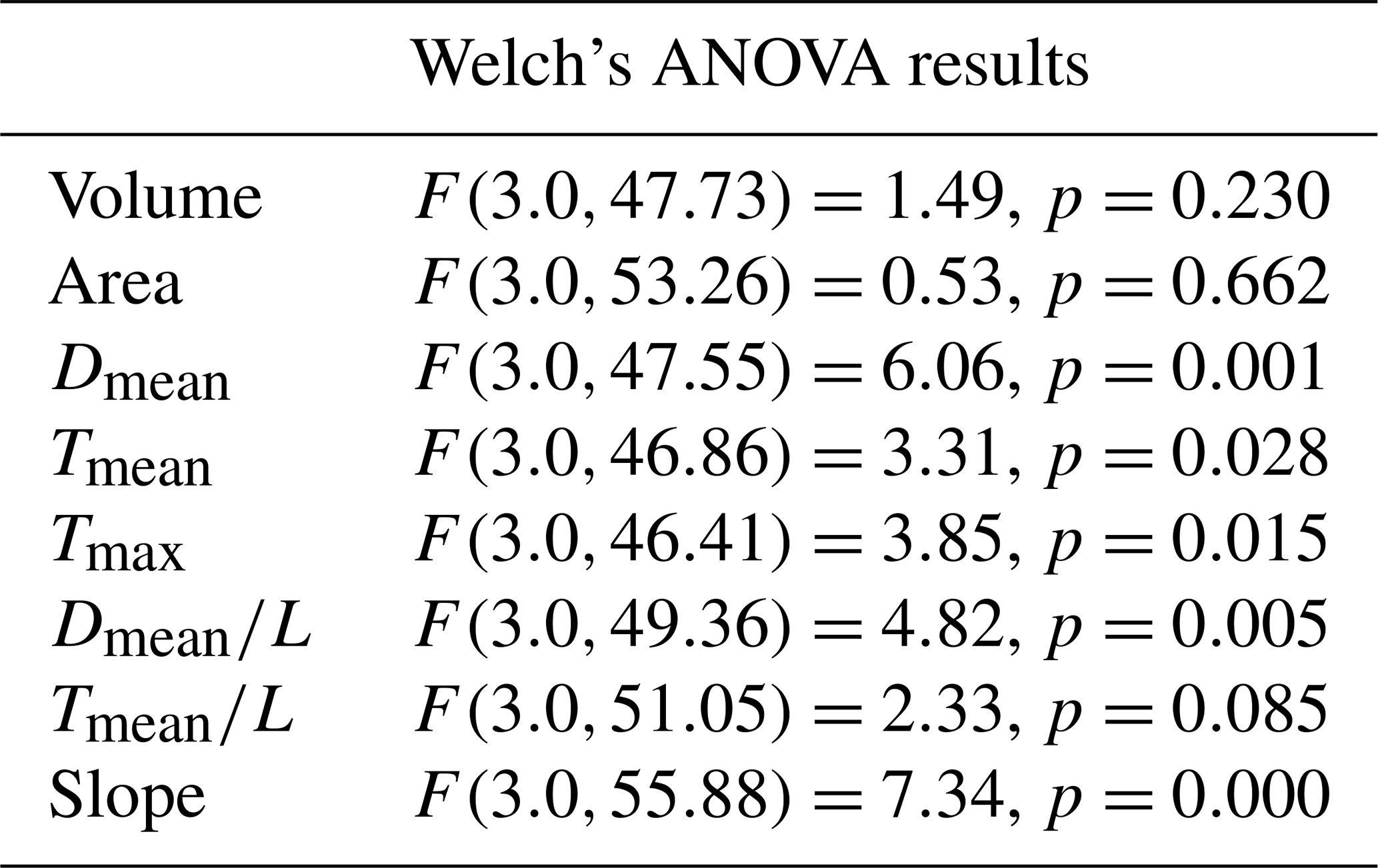
Figure 10 shows similar results but uses the average number of trees within a 10 m radius for each of the scar cells to group the data. Except for the volume, area and $T_{\text{mean}}/L$ distributions, the grouping based on the average number of trees in a 10 m radius results in statistically significant differences between distributions of the scar parameters of the groups (Table 6). However, the analysis also shows that there is only a difference between the group that on average has no neighbouring trees and the other groups. If the group without trees is filtered out, the groups do not show any differences. This was also shown with ANOVA tests on the different parameters, using a filtered dataset where the group without trees was left out. The p-values of these ANOVA tests all fell above 0.05, including for an ANOVA test on the relationship with the pre-failure slope of the scar.

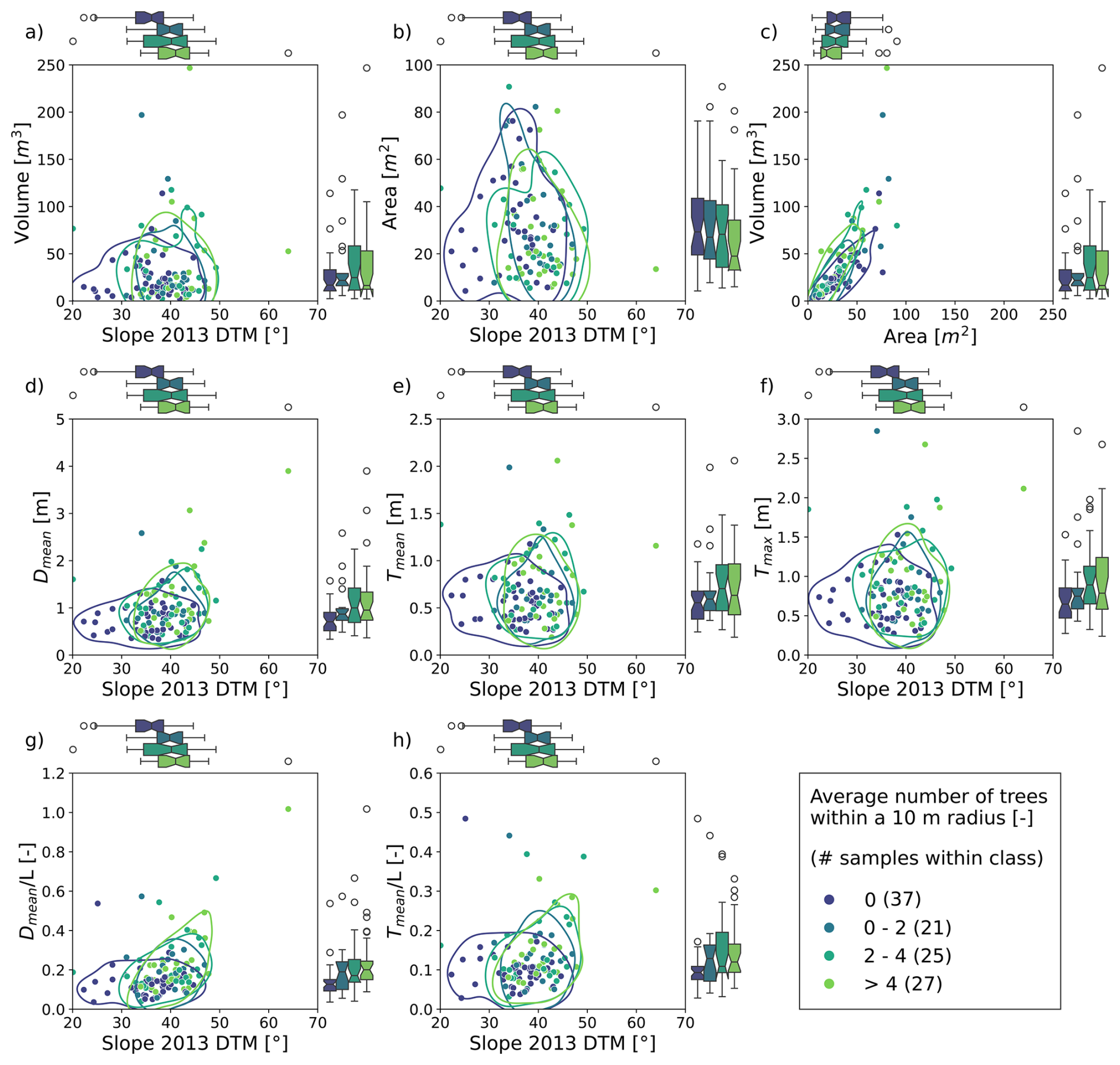
Figure 10 Analysis of the relationship between scar morphology and the average pre-failure slope of the scars (from the 2013 DTM data), coloured by the average number of trees within a 10 m radius calculated from each of the scar cells. The contour boundaries show the 75th percentile boundary of the binned average tree number subsets. The plotted parameters are (a) the scar volume, (b) the scar area, (c) the scar volume against the scar area (instead of the 2013 DTM slope), (d) the mean depth, (e) the mean thickness, (f) the maximum thickness, (g) the mean depth to length ratio and (h) the mean thickness to length ratio.

Table 6 ANOVA results on the grouped data and parameters from Fig. 10.

The analysis of the landslide topographic profiles with regards to its forest classification is given in Fig. 11. The plots of the topographic profiles along and across the slope direction show that the median thickness profile of the landslides in forests is deeper than the median thickness profile of the landslides outside the forest. In addition to the general difference in thickness, the along-slope profile also indicates that the scar head profile of the landslides within the forest is generally steeper than from landslides outside the forest. Within the interval of −7 to 7 m, the median across slope profile has a root mean squared deviation (RMSD) of 0.12 m. For the interval −2 to 2 m this increases to 0.18 m. For the along the slope profiles, the difference of the median profiles has a RMSD value of 0.11 m for the interval −7 to 15 m. For the interval −2 to 2 m, this increases to 0.20 m.

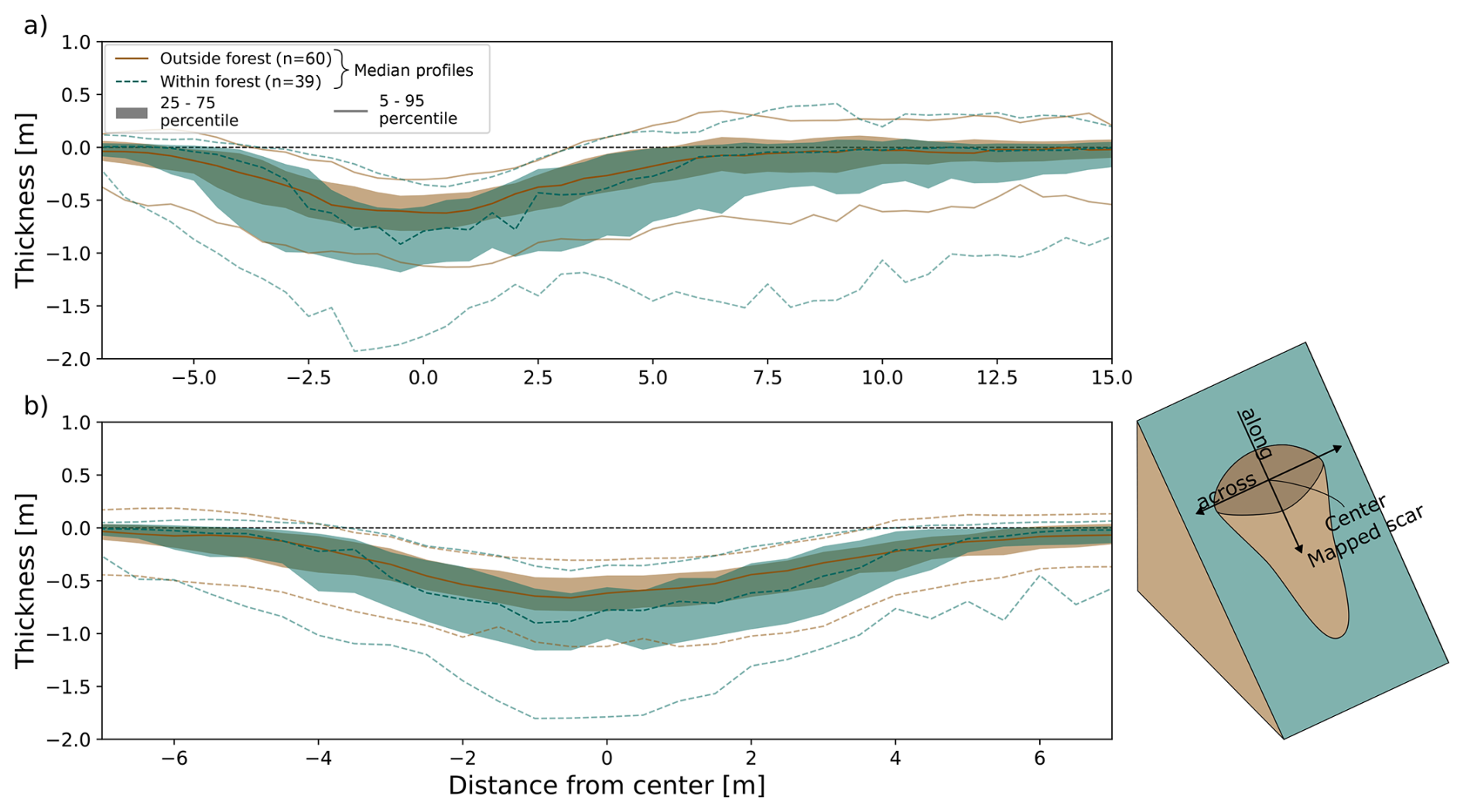
Figure 11 Topographic profiles from the thickness dataset of the scars within the forest (green) and outside the forest (brown). (a) shows the profile along the slope direction and (b) across the slope direction. The x axis indicates the distance of the profile point from the centroid of the scar.

Lastly, Fig. 12 shows the relationship between the topographic profiles of the landslides and the closest tree distance and the average slope of the pre-event DTM. The graphs show that both the slope and the closest tree distance have an impact on the profiles of the landslides. With a smaller closest tree distance, the landslide profiles are generally deeper than for larger tree distance values. Additionally, the scar profiles at distances far away from trees (>15 m) are flatter than other scar profiles. For the slope of the pre-event DTM, the plots show that a larger slope value is generally related to narrower and shorter scar profiles.

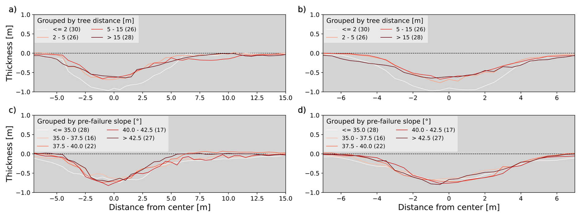
Figure 12 Median profiles from the thickness dataset with a grouping of the landslides according to their closest tree distance (a, b) and the average slope in the 2013 DTM (c, d). The plots on the left (a, c) show the landslide profiles along the slope direction and the plots on the right (b, d) the profiles across the slope direction.

5 Discussion

5.1 Performance of the landslide detection and scar mapping with the RF model

The performance metrics show a good performance of the RF model (AUC: 0.94) and the subsequent segmentation of the RF output (D2PC: 0.26 with TPR of 73.8 %). The metrics show that there is a general underestimation of the landslide area and occurrence in the final inventory, however, this is traded off with a very low, pixel-based FPR. Since one of the main goals in developing the RF workflow was a higher degree of automation, a lower false positive rate was preferred over a higher TPR. A lower false positive rate also ensures that a higher certainty can be attached to the final inventory.

The degree of automation was a very important focus in the creation of the landslide scar detection and segmentation workflow. A higher degree of automation also brings with it a better transferability and a higher robustness of the results from the statistical analysis, since it lowers the impact of human decision-making or errors on the analysis. It was not possible to create a fully automated workflow, as the output of the detection and segmentation workflows still had high false positive rates. However, the human intervention within the developed workflow was limited to only the exclusion or inclusion of certain landslides. Since the output from the convergence index was used directly in the scar representation, the human intervention did not change the scar boundaries.

With regards to the validity of the scar boundaries in this study, it should be said that although there might be some discrepancies in the delineation of scars in our approach compared to more traditional landslide mapping approaches, the effects of these discrepancies (e.g., the underestimation of scar area) do not affect the conclusions in the comparison of landslides within and outside of the forest. It can be assumed that the under- and overestimation of the scar sizes is consistent across the different forest classifications. In addition, it should also be pointed out that the found differences in the landslide profiles and depth derivatives are not affected by the scar construction.

5.2 Morphological and topographic profile differences of landslides within and outside of forest in the RF inventory

The distributions of the morphological landslide parameters and the topographic profiles of the scars in the RF inventory, showed that there are distinct differences between landslides within the forest and landslides located outside forests. From the morphological characteristics it was shown that there is a statistically significant difference in the slope of the scars in the pre-event DTM, the depth and thickness of the scars, and their $D_{\text{mean}}/L$ and $T_{\text{mean}}/L$ ratios, with significantly higher slopes, deeper scars and higher thickness- and depth-to-length ratios for landslides located within the forest. It should be noted that the higher slope angle was expected due to prevalence of steeper slopes within the forest in the study area. No relationship was found between the area and volumes of the scars and the binary classification of their location respective to the forest. However, with the more detailed analysis of the relationship of the morphological parameters with the tree distance of the scars it was found that there is also a significant relationship between the scar volume and the distance of the nearest tree. The plots of the topographic profiles of the scars also showed that the scar thickness is larger for landslides located closer to trees. Interestingly, these plots also showed that the along-slope profile of the scars in the forest is steeper than those from scars outside the forest, suggesting that the scar length of these scars is also shorter. The analysis investigating the relationship of these differences with the number of trees within the scar neighbourhood (Fig. 10), showed that the found differences are only related to the presence of trees within a certain radius. This indicates distance to trees surrounding the scar has a stronger relationship with the scar characteristics than the number or density of trees surrounding the scar.

The strong relationship of the distance to a tree parameter with the morphometric characteristics of the scars indicates that the morphometric parameters are affected by their location within the influence zones of the trees. This strong relationship could for example reflect the decreasing rooting depth away from the tree, which results in a decreasing depth at which the tree roots provide additional stability to the slope with root cohesion (Preti, 2013). Additionally, it could also reflect the degree in which a tree has influenced the hydrological properties of the soil in its vicinity through bio-ecological processes, with decreasing effects further away from the tree. A more thorough analysis of the exact vegetation related processes affecting the scar characteristics would require more information on the forest and tree characteristics than is currently available. To effectively analyse this, further research should consider the relationship of the scar characteristics with different tree species, but more importantly also tree-specific datasets such as tree age, tree height and local growth conditions.

To investigate if other factors, unrelated to the forest cover, are influencing the found differences in landslide characteristics, an additional analysis was performed on the relationship between the scar characteristics and the average pre-failure slope values of the scars, as extracted from the 2013 DTM. The resulting scatter-plots of this are given in Appendix B and the corresponding ANOVA results of the morphological parameter distributions with a classification according to pre-failure slope classes are given in Table 7. The analysis shows the pre-failure slope values only have a significant relationship with the $D_{\text{mean}}/L$ and $T_{\text{mean}}/L$ ratios of the scars. This rules out the effect of the slope on the other characteristics of the landslide scars, but does not rule out if other factors unrelated to the forest cover are influencing the differences in landslide characteristics. Examples of this could be differences in soil type or soil structure, which could influence the geotechnical and hydrological conditions of the soil. In addition, it should also be noted that the profiles could reflect differences in erosional processes that occurred after the event.

Table 7 ANOVA results of the morphological scar parameter distributions with a grouping by average pre-failure slope of the scars. Full scatter plots of the distributions are given in Fig. B1.

5.3 Landslide characteristics in other studies

The areas of the scars in this study are significantly lower than what is reported in other studies (Emberson et al., 2022; Malamud et al., 2004). However, this discrepancy is expected due to the different approach that was used for the landslide mapping in this study. Most studies reporting statistics on landslides constructed their inventories from aerial or satellite imagery. Besides this, the decision on which sections of the landslides are included within the landslide boundary (only the scar, the full erosional area or also the depositional area) can vary significantly across different studies (Guzzetti et al., 2012). In addition, most inventories also do not focus on a specific landslide type and include both large deep-seated landslides as well as small shallow landslides (Reichenbach et al., 2018). This makes it very difficult to compare information on landslide parameters across different studies and has also been reported before by other studies (Ardizzone et al., 2007; Zieher et al., 2016). Within the current study this problem is also displayed by the differences of the BFW and RF inventories.

With regards to the comparison of landslides within and outside of the forest, a study by Roering et al. (2003) shows that the root cohesion is highly related to the spacing, size and condition of trees and thus the location of landslides, in agreement with the found importance of the tree distance parameter in the present study. Only a few studies provide insight into how the forest cover affects other landslide characteristics. Rickli and Graf (2009) compared the area, depth and volume values of landslides in forests and outside of forests from multiple study sites in Switzerland. They did not find consistent results about the area, volume and depth parameters, as the direction and significance of differences in area, volume and depth between landslides inside and outside of forests varied across the different study sites. Koyanagi et al. (2020) investigated earthquake induced landslides and found that forested landslides are smaller than those outside the forest. In addition, they also found that forested landslides are deeper than those outside the forest. They did not test the significance of these differences. However, the difference in landslide depth within the forest was more than 2 times the mean landslide depth outside of the forest for one of the sites. It could be that these differences in landslide depth for forested landslides found by Koyanagi et al. (2020) are related to the difference in processes behind earthquake triggered and rainfall-triggered landslides. Additionally, it should also be noted that comparability across studies is limited since no standardized forest definitions are used.

6 Conclusions

In this study we developed a well performing semi-automatic landslide detection and mapping workflow that also explicitly considers landslides under forest canopy cover. The main aim of this study was to use this semi-automatic workflow for the analysis of landslides in forests and the effect of the forest cover on landslide morphology and their topographic profiles. To analyse this, the study focused on an extreme, short-burst rainfall event that triggered a large number of shallow landslides in the Sellrain valley, Tyrol (Austria). The results of the analysis show that there are significant differences between landslides inside and outside of forests for the studied event, with significantly larger depths, larger thicknesses and higher pre-failure slope values for landslides located in forests. An analysis with forest structure parameters (i.e., the distance to the closest tree and the average number of trees within a 10 m neighbourhood radius of the scar cells) also found significantly larger landslide source volumes (i.e., landslide magnitudes) for landslides located closer to the trees. Furthermore, the analysis with the forest structure parameters also showed that these differences were mainly related to the distance to the closest tree, most likely reflecting the relationship of the landslide characteristics with the spatial distribution of root cohesion.

It was possible to determine that there are significant differences between landslides occurring within and outside of the forest. However, inferring what processes are underlying these differences would require data from more well-documented events, including comprehensive soil and forestry information. Since the current study already showed a strong link between the distance to the closest tree and the landslide characteristics, further research could focus on how the threshold of this distance is impacted by different soil types and if trees of various species at different stages of development and under different growing conditions also show different distance thresholds. In conclusion, the results provide a better understanding of how the negligence of landslides under forest cover in inventories impact inventory-derived statistics, showing that landslide prediction models trained with biased inventories will not only underestimate the occurrence of landslides in the forest but also the magnitude of these landslides. Additionally, this study enhances our understanding of the impacts of forest on landslide processes and their protective function.

Appendix A

The hyperparameter set-up for the RF landslide detection model is given in Table A1. The final optimal hyperparameter set-up is also given in this table and was chosen after 300 trials based on the highest AUC score, resulting in a more balanced model performance.

Table A1 Tuned hyperparameters for the random forest landslide detection model with the used ranges and the final values.

The workflow for the segmentation algorithm that was applied to the probability output of the RF detection model, for further false positive filtering, is given in Fig. A1. The paramter ranges for the calibration of the set-up are given in Table A2. The parameters were also tuned with Optuna and the final parameter combinations were chosen after 1200 model runs, based on the highest D2PC value. The final parameter values are also given in Table A2.

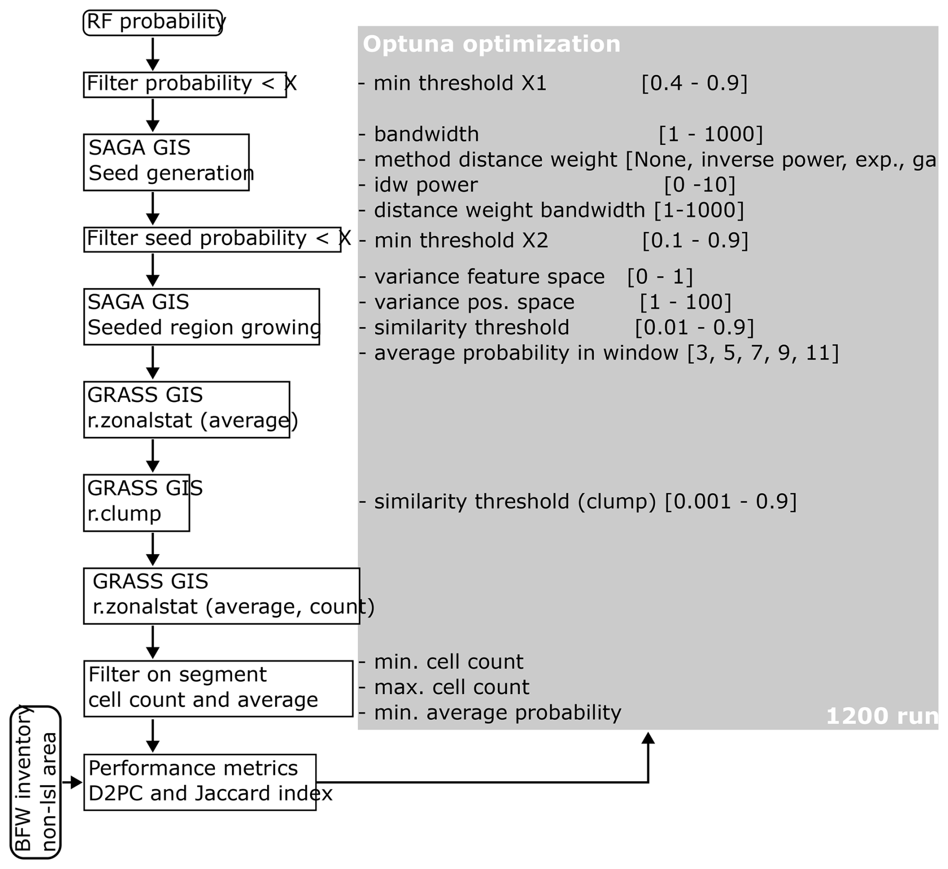
Figure A1 Workflow for segmentation and filtering of the probability output of the random forest landslide detection model.

Table A2 Overview of the parameters and their value ranges used in the segmentation workflow, with the final values given in the rightmost column.

Appendix B

In addition to the relationship between the forest structure parameters and the morphology of the scars, it was also tested how the scar morphology is impacted by the pre-failure slope value, as extracted from the 2013 DTM. The analysis was performed similarly to the analyses of the relationship between the scar characteristics and the forest structure parameters. Instead of the forest structure parameters, the analysis used the average pre-failure slope value of the scars from the 2013 DTM. The results of this analysis are given in Fig. B1 and Table 7. The results show that the pre-failure slope only has a relationship with the $D_{\text{mean}}/L$ and $T_{\text{mean}}/L$ values of the scar.

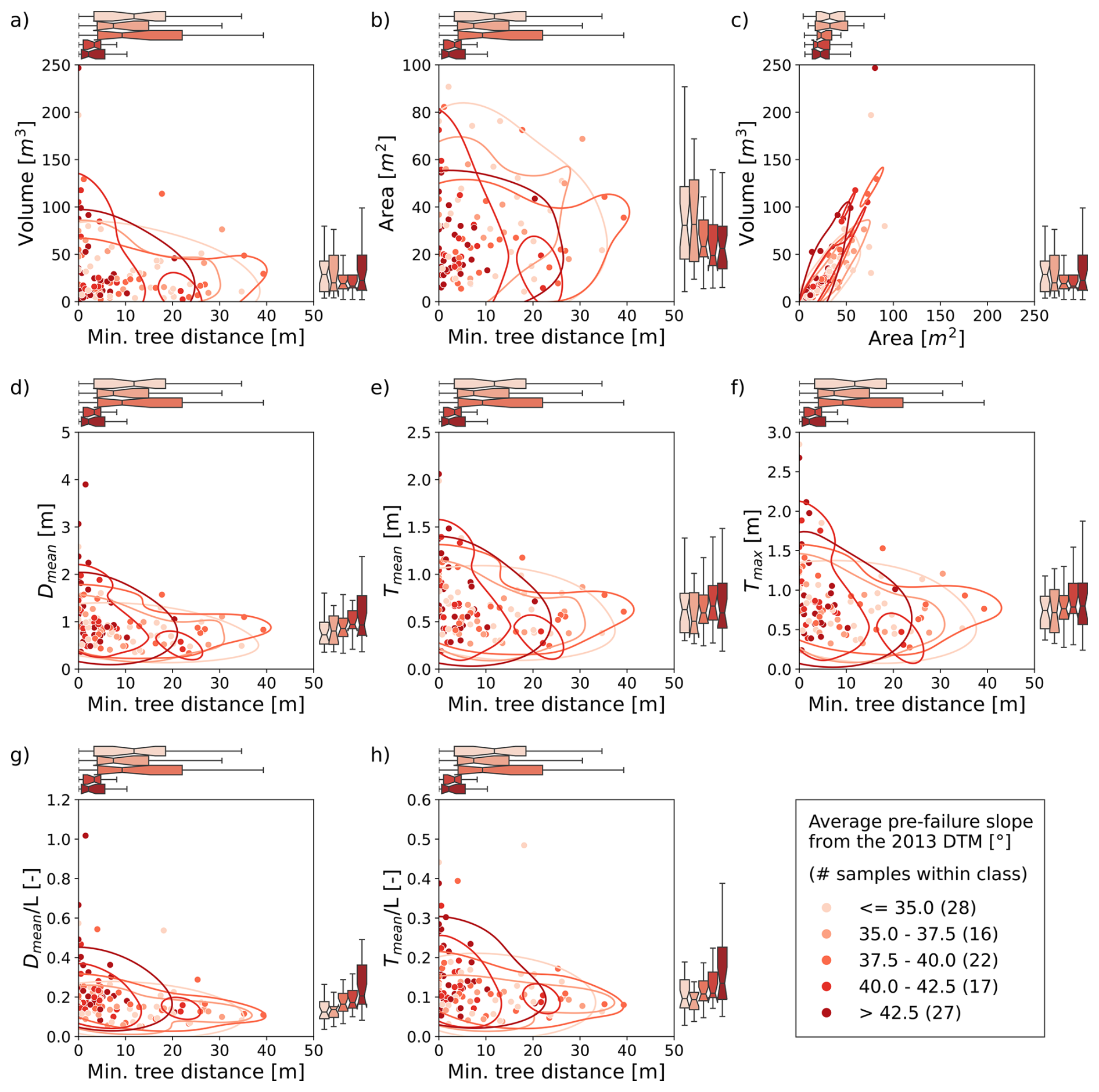
Figure B1 Analysis of the relationship between the scar morphology and minimum tree distance of the scars, coloured by the average pre-failure slope value of the scars from the 2013 DTM. The contour boundaries show the 75th percentile boundary of the binned average pre-failure slope values. The plotted parameters are (a) the scar volume, (b) the scar area, (c) the scar volume against the scar area (instead of the minimum tree distance), (d) the mean depth, (e) the mean thickness, (f) the maximum thickness, (g) the mean depth to length ratio and (h) the mean thickness to length ratio.