Shaping shallow landslide susceptibility as a function of rainfall events

This paper tests a multivariate statistical model to simulate rainfall-dependent susceptibility scenarios of shallow landslides. To this end, extreme rainfall events spanning from 1977 to 2021 in the Orba basin (a study area of 595 km² located in Piedmont, northern Italy) have been considered. First of all, the role of conditioning and triggering factors on the spatial pattern of shallow landslides in areas with complex geological conditions is analysed by comparing their spatial distribution and their influence within logistic regression models, with results showing that rainfall and specific lithological and geomorphological conditions exert the strongest control on the spatial pattern of landslides.

Different rainfall-based scenarios were then modelled using logistic regression models trained on different combinations of past events and evaluated using an ensemble of performance metrics. Models calibrated on multiple events outperform the ones based on a single event, since they are capable of compensating for local misleading effects that can arise from the use of a single rainfall event. The best-performing developed model considers all the landslide-triggering rainfall scenarios and two non-triggering intense rainfall events, with a score of 0.90 out of 1 on the multi-criteria TOPSIS-based¹ performance index.

Finally, a new approach based on misclassification costs is proposed to account for false negatives and false positives in the predicted susceptibility maps.

Overall, this approach based on a multi-event calibration and on a misclassification cost analysis shows promise in producing rainfall-dependent shallow landslide susceptibility scenarios that could be used for hazard analyses and early warning systems and could assist decision-makers in developing risk mitigation strategies.

1 Introduction

Shallow landslides are a widespread phenomenon that affects many regions of the world (Petley, 2012). In Italy, according to the last national report on landslides and floods, almost 8 % of the country is affected by landslides, of which 15 % are classified as rapid flow and 6 % as shallow landslides (ISPRA, 2021). According to Cruden and Varnes (1996), these are shallow landslides, mainly translational, with a thickness ranging between 0.5 and 2 m (Bandis et al., 1996; Mason and Rosenbaum, 2002). Shallow landslides are generally triggered by rainfall events, which cause an increase in pore water pressure or a loss of apparent cohesion generated by suction (Caine, 1980; Crosta and Frattini, 2003; Fredlund et al., 1978; Iverson, 2000; Lu and Godt, 2008). Despite their limited initial volume, these landslides may be characterized by a high density per unit area and can evolve into debris flows. The high velocity and the difficulty of prediction due to the almost complete lack of premonitory signs (Campbell, 1975; Frattini et al., 2009; Montrasio et al., 2016) make these phenomena seriously dangerous in terms of life and economic losses (Trigila and Iadanza, 2012).

A common definition of landslide hazard is “the probability of occurrence within a specific period of time and within a given area of a potentially damaging phenomenon” (Varnes, 1984), requiring the quantification of the magnitude and the spatial and temporal probability for an instability event to occur. The variables that control landslide hazards are commonly distinguished into conditioning and triggering factors. Conditioning factors are generally assumed to have no temporal dependence and are responsible for “where” a landslide might occur, while triggering factors are event-related and control “when” a landslide might occur (Crosta and Frattini, 2003; Lombardo et al., 2020; Wu and Sidle, 1995), although their spatial properties (e.g. distribution of intensity or cumulative rainfall during a rain event) play a key role in determining the location of landslides.

The spatial likelihood of shallow landslide occurrence is addressed through landslide susceptibility models, based on either physically based or machine-learning techniques. Physically based techniques for shallow landslides often combine the infinite-slope model with hydrogeological models, which require many different input data; for this reason, they are more frequently applied at the site scale (Baum et al., 2008; Montgomery and Dietrich, 1994).

Machine-learning methods search for functional relationships between the conditioning factors and the distribution of landslides, obtained from inventories of past events (Carrara, 1983; Goetz et al., 2015; Huang et al., 2020; Reichenbach et al., 2018; van Westen et al., 2008). Susceptibility models are usually considered time independent, meaning that the likelihood of landslides occurrence does not vary in time (Jones et al., 2021; Lombardo et al., 2020). However, many authors demonstrated that this assumption is often violated on both long (hundreds or thousands of years) and short (tens of years) timescales, especially in view of climate changes (Hungr, 2016; Samia et al., 2018). The “when” problem has typically been addressed by using rainfall thresholds or physically based models. Rainfall thresholds describe the rainfall intensity, duration, or cumulative event precipitation that may trigger landslides for a particular area (Caine, 1980; Crosta, 1998; Guzzetti et al., 2007). This approach has usually disregarded soil features and morphometric conditioning factors, such as the geotechnical features of the involved materials, until recent times, when hydrogeological effects started to be included in the analyses, e.g. through the consideration of the soil water content prior to the triggering event (Bogaard and Greco, 2018; Marino et al., 2020). Some authors started testing approaches to address both the “where” and the “when” questions in the context of early warning systems. For example, Kirschbaum and Stanley (2018) used a fuzzy overlay model to combine static explanatory variables into a susceptibility map. This information was then incorporated into a heuristic decision tree model together with dynamic variables such as antecedent precipitation, giving a model capable of indicating potential landslide activity in near real-time. Segoni et al. (2018b) combined rainfall thresholds and susceptibility maps into a hazard matrix, while Bordoni et al. (2021) integrated rainfall thresholds and antecedent soil humidity with a susceptibility model in order to forecast the spatial and temporal probability occurrence of shallow landslides. Camera et al. (2021) included intense rainfall and snowmelt in a landslide susceptibility model trained over multiple landslide inventories and different meteorological conditions, making it potentially more robust to investigate the effects of climate changes. Knevels et al. (2020) and Maraun et al. (2022) included 5 d cumulated rainfall and maximum 3 h rainfall intensity to model landslides associated with an extreme rainfall event, and then they applied their findings to an event storyline approach to analyse the future landslide occurrence probability under climate changes. Moreno et al. (2024) integrated static and time-dependent controlling factors into a generalized additive mixed model (GAMM) to forecast shallow landslides in space and time, showing that both short-term (2 d) and medium-term (14 d) cumulative precipitation increases the model capabilities.

Yet, the integration of static and time-varying factors into machine-learning models still remains challenging, but it could become a powerful instrument to better understand the connection between a variation in the time-dependent controlling factors and landslide triggering, thus helping at improving landslide prediction in a changing climate.

An important issue for the application of susceptibility models is the evaluation of their performance. For models that predict binary stable and unstable slopes, it is necessary to choose a cut-off value below which the predicted susceptibility values are treated as 0 and above which the values are treated as 1 (Beguería, 2006; Brenning, 2005; Frattini et al., 2010; Goetz et al., 2015; Guzzetti et al., 1999). This results in a contingency matrix quantifying the total number of correctly and incorrectly classified units. From this matrix, it is possible to assess the performance of the model by using several performance statistics, such as the accuracy (i.e. the ratio between the correctly classified samples and the total number of samples), the precision (i.e. the ratio between the true positive samples and all the positively classified samples, meaning the sum of the true positives and the false positives), the true positive rate (TPR) (i.e. the ratio between the true positive and all the positives, meaning the sum of the true positives and the false negatives), the false positive rate FPR (i.e. the ratio between the false positives and all the negatives), the threat score (Gilbert, 1884), Pierce's skill score (true skill statistic; Peirce, 1884), Heidke's skill score (Cohen's kappa; Heidke, 1926), and the odd ratio skill score (Yule's Q; Yule, 1900).

However, the choice of the cut-off value is a complex problem; therefore, the performance is frequently evaluated by using cut-off-independent methods, such as the receiver operating characteristic (ROC) curves (Frattini et al., 2010; Hosmer and Lemeshow, 2000; Provost and Fawcett, 2001) or the precision–recall (PR) curves (Davis and Goadrich, 2006; Raghavan et al., 1989; Saito and Rehmsmeier, 2015). The ROC curve represents the FPR and TPR obtained for different cut-offs. The area under the curve (AUROC) can be used to quantify the overall quality of the model (Hanley and McNeil, 1982). However, ROC curves can overestimate the performance of a model when the distribution of the input classes is highly skewed. For this reason, the precision–recall (PR) curves have also been used (Nam et al., 2024; Yordanov and Brovelli, 2020; Zhao et al., 2022), which plot the precision (i.e. the proportion of true positives among the positive predictions) against the TPR. However, unlike the ROC curve, the value under the PR curve is not directly interpretable for model evaluation, especially because of a non-universal baseline performance, which depends on the class distribution, and a non-linear interpolation of precision values. Nevertheless, PR analysis can be adapted to be used similarly to the ROC analysis by using precision–recall–gain curves (PRG), which make use of the F–gain score, a linearized version of the F₁ score, to properly take baselines into account (Flach and Kull, 2015).

One important consequence of the choice of the cut-off value is the generation of false and missed alarms, meaning the situations in which the model predicts a landslide in a specific area or time but no landslide actually occurs or the case in which a landslide takes place but the model fails to predict it. False and missed alarms come with associated costs. For example, false alarms may lead to unnecessary evacuations or resource allocation, and they can reduce trust in the model capabilities, while missed alarms result in unpreparedness and potentially severe consequences, including property damage, loss of life, or economic impacts. Therefore, the performance of the model can be evaluated by assessing the expected misclassification costs through the cost curves (Drummond and Holte, 2006; Frattini et al., 2010), with an approach that allows for the choice of the cut-off value that minimizes the expected costs (Sala et al., 2021).

A multivariate statistical analysis for the Piedmont area of the Orba basin (northern Italy) has been developed in this paper, considering rainfall scenarios spanning from 1977 to 2021, to investigate the correlation between landslide distribution and the spatial pattern of conditioning and triggering factors. Different logistic regression models were trained for different landslides and rainfall scenarios, and their performance was evaluated through an ensemble of performance metrics, leading to an optimal choice of the best model for scenario-based problems or early warning.

This work allows us to address the following research questions:

• To what extent the pattern of shallow landslides is controlled by the characteristics of the rainfall event in areas with complex geological conditions?

• How can rainfall be used within a statistical model to produce instability scenarios for different rainfall events?

• Which is the best strategy to train a statistical model based on an ensemble of rainfall events?

• Which is the most significant classification scheme to produce a susceptibility map for early warning purposes?

The novelty of this work lies in the definition of a critical selection strategy of the optimal ensemble of rainfall events to produce a susceptibility map that may be helpful for scenario-based problems and early warning purposes. Moreover, a new methodology is proposed for the classification of the regression results, used for the realization of the final resulting maps.

2 Materials and methods

2.1 Study area

The Orba basin is located between the Langhe and Alto Monferrato Hills of Piedmont region, north-western Italy. This area has been affected by several high-magnitude floods and severe slope instabilities during the last century, caused by intense rainfall events (Mandarino et al., 2021). The study area has an extension of 595 km², and it is situated between 80 and 1170 m a.s.l. The main river of the basin, the Orba River, flows northward from the Ligurian Apennines to the confluence with the Bormida River, a right tributary of the Po River. The study area overlaps magmatic and metamorphic lithotypes in the southern part – mainly peridotites, serpentinites and serpentine-schists, meta-gabbros, and meta-sediments belonging to the Voltri Massif and the Sestri-Voltaggio Zone (Piana et al., 2017) – while in the central part of the area the sedimentary sequence of the Tertiary Piedmont Basin (TPB) outcrops. The TPB evolved from the Late Eocene to the Late Miocene over the inner part of the Alpine wedge (Coletti et al., 2015) and is mainly represented in the area by conglomerates, sandstones, and marls. The northern sector of the basin presents Quaternary fluvial deposits belonging to the Alessandria–Tortona floodplain. The morphology of the area is strongly controlled by the TPB sedimentary succession: where the strata are harder, the landscape presents hilly reliefs with an asymmetric profile resulting from the monoclinal bedding of marly-silty and sandy-arenaceous alternations (Luino, 1999), which are part of a monoclinal structure striking WNW–ESE that imposes a dipping of approximately 30° (Luino, 1999; Mason and Rosenbaum, 2002), while lowered areas modelled by fluvial erosion are present where the lithologies are more erodible. When the dipping of the strata becomes gentler, the morphology becomes more uniform and characterized by a dense hydrographic network. The mean annual temperature is 13°, and the average annual precipitation ranges from around 600 mm yr⁻¹ in the northern part to 1600 mm yr⁻¹ in the southern part, with autumn as the rainiest season (Fioravanti et al., 2022; Luino, 2005). Land use is primarily forest (45 %), with crops and meadows (24 %) near the confluence with the Po River (Land Cover Piemonte, https://geoportale.igr.piemonte.it/cms/progetti/land-cover-piemonte, last access: 21 October 2023).

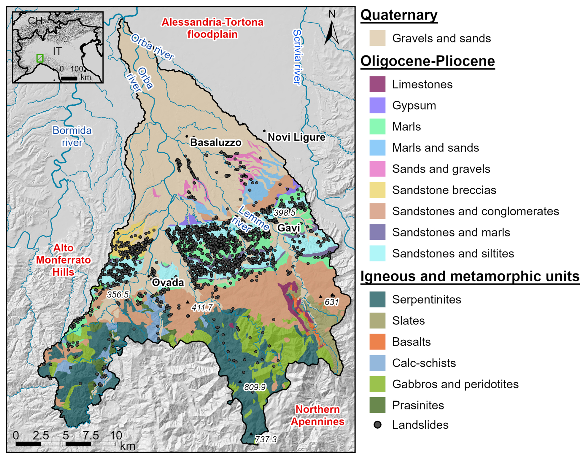
Figure 1 Location of the Orba basin, with the spatial distribution of shallow landslides observed in three different events and with the main lithologies.

2.2 Data

2.2.1 Rainfall events and landslide inventories

The inventories related to three different landslide events that occurred in 1977, 2014, and 2019 were used for the subsequent analyses. Data relative to the events of 1977 and 2014 are available online (SIFRAP, Sistema Informativo sulle FRane in Piemonte, handled by Regional Environmental Protection Agency of Piemonte – ARPA Piemonte) and were compiled through the analysis of Google Earth images, national and regional orthophotos, published event maps, and field reconnaissance, while the most recent event was directly provided for this project by ARPA Piemonte (unpublished data). The 2014 and 2019 inventories include polygons of each single shallow landslide, while the 1977 inventory represents clusters of shallow landslides as polygons.

The first shallow landslide event was triggered by heavy rainfall at the beginning of October 1977. Between 6 and 7 October, more than 400 mm of rain fell in less than 24 h, causing flooding, bank and riverbed erosion, debris flows, and soil slips (INTERREG IIC, 1998). The second shallow landslide event was triggered in October 2014 with more than 420 mm of rain in less than 12 h, as recorded at the Gavi meteorological station on 13 October, for which the mean annual total rainfall is 1000 mm (calculated for the 1991–2020 time interval, ARPA Piemonte). The third shallow landslide event occurred in late October 2019. In the afternoon and evening of 21 October, more than 400 mm of rain (Gavi station) fell in less than 12 h, resulting in a very high-magnitude flood and widespread shallow landslides (ARPA Piemonte, 2019).

In addition to these three landslide-triggering rainfall events, two intense precipitation events (2016 and 2021) that were not associated to landslides were selected in order to test the capabilities of the models to discriminate between triggering and non-triggering rainfall characteristics. The 2016 event hit the Piedmont region with strong and persistent rainfalls between 21 and 25 November, and it triggered almost 1000 landslides, none of which were in the Orba basin. Indeed, the peak of the cumulative precipitation was localized more southward compared to the ones previously described, with up to 400 mm of rain in the southern edge of the Orba basin. The other event happened from 3 to 5 October 2021. The Ligurian-Piedmont watershed was the most affected area, with a peak of 472 mm of rain in 12 h recorded in the south-western part of the area. The total precipitation in the Orba basin was up to 750 mm in the south-western edge of the basin. The daily maximum rainfall intensities and the yearly cumulative rainfall values for all the considered events are reported in Fig. 2.

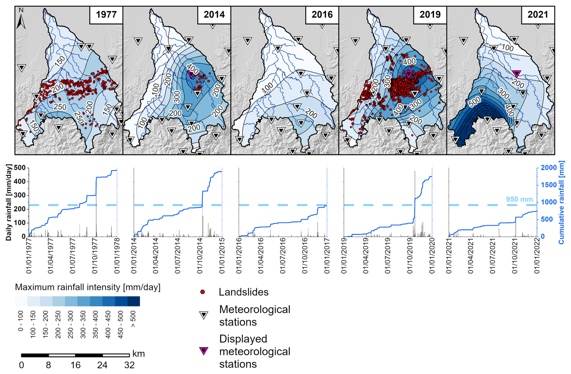
Figure 2 Maximum daily rainfall intensity and landslide distribution during the considered events, reconstructed by interpolation of values measured by the meteorological stations on the ground, that led to landslide triggering in the Orba basin. Graphs report the daily and cumulative rainfall for the year in which the shallow landslides were triggered. Dashed lines represent the mean annual rainfall for the basin of interest (ARPA Piemonte).

For all the inventories, a non-cumulative logarithmic binned landslide size probability density distribution was developed:

$$\begin{array}{}\text{(1)}& p\left(A\right)={\displaystyle \frac{\mathrm{1}}{N_{\mathrm{tot}}}}{\displaystyle \frac{\partial N}{\partial A}},\end{array}$$

where ∂N in the number of landslides with an area between A and $A+\partial A$, and N_tot is the total number of landslides within a study area (Malamud et al., 2004). Following Frattini and Crosta (2013), a Pareto distribution was fitted to the probability density above a minimum size cut-off (Fig. 3):

$$\begin{array}{}\text{(2)}& p\left(A\right)=\mathit{\alpha }{c}^{\mathit{\alpha }}{A}^{-\mathit{\alpha }}{}^{-\mathrm{1}}c>\mathrm{0},\mathit{\alpha }>\mathrm{0},A\mathit{ϵ}[c,\mathrm{\infty }).\end{array}$$

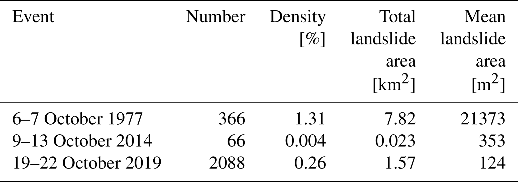
Using the maximum likelihood estimation, the distribution parameters were estimated, obtaining a good fitting for landslides larger than 500 m², with the best fitting results for landslides greater than 1000 m². The scaling exponents α vary between 1.5 and 2.6, values that are higher than most of those reported in the literature but still in the range (Van Den Eeckhaut et al., 2007).

Table 1 Statistical parameters describing the landslide events in the study area.

2.2.2 Landslide conditioning and triggering factors

The conditioning factors used in the following analyses include seven morphometric parameters, lithology, soil grain size distribution, and land use (Fig. S1 in the Supplement). The morphometric parameters were extracted using ArcGIS Pro 3.1.0 © from a 5 m resolution digital terrain model (DTM) acquired using a uniform methodology (lidar) at Level 4 standard, with an elevation accuracy of ±0.30 m (±0.60 m in areas of lower precision, corresponding to wooded and densely urbanized areas), provided by Piedmont region. The morphometric factors are slope angle, northernness, easternness, profile curvature, planar curvature, total curvature, and flow accumulation. Lithological information was obtained from the geological map of the Piemonte region, at a scale of 1 : 250 000 (Piana et al., 2017). The units have been reclassified by aggregating geo-stratigraphic units with comparable lithological and litho-technical characteristics (Table S1 in the Supplement), resulting in 16 lithological classes (Fig. 1: gravels and sands, limestones, gypsum, marls, marls and sands, sands and gravels, sandstone breccias, sandstones and conglomerates, sandstones and marls, sandstones and siltites, serpentinites, slates, basalts, calcschists, gabbros and peridotites, and prasinites).

Information relative to the soils grain size distribution was retrieved from the SoilGrids maps (Poggio et al., 2021), reporting soil properties for the entire globe with a resolution of 250 m. SoilGrids models were obtained through the application of machine learning to soil data collected worldwide.

The land use was obtained from the 10 m resolution Land Cover Piemonte map, which integrates information collected between 2018 and 2022 (https://geoportale.igr.piemonte.it/cms/progetti/land-cover-piemonte, last access: 21 October 2023). 12 different land-use classes were used, namely arable land, areas with sparse/absent vegetation, artificial non-agricultural green areas, heterogeneous agricultural areas, inland waters, mining areas, permanent crops, permanent lawns, road network, shrubby/herbaceous areas, urbanized and productive areas, and woods. Besides the predisposing factors, several rainfall parameters potentially responsible for the shallow landslides triggering were also included into the analysis. These parameters were obtained by interpolating daily rainfall data collected at 39 and 51 gauging stations for the 1977 and 2014/2019 rainfall events, respectively, with a natural neighbour technique, at a spatial resolution of 5 m. In particular, the maximum daily rainfall intensity (mm d⁻¹, Fig. 2) and the antecedent cumulative rainfall (mm, Fig. S2) over 10, 30, 60, and 90 d (Smith et al., 2023) as a proxy for soil water content prior to the event (Guzzetti et al., 2007), which can increase the likelihood of failure (Bogaard and Greco, 2018; Thomas et al., 2018), were extracted for each event. Maximum daily rainfall intensities were normalized by the daily rainfall with a return period of 10 years, provided by ARPA Piemonte with a grid resolution of 250 m, while the total and antecedent rainfall values were normalized by the mean annual precipitation (1991–2020) within the study area (Fig. S3). Data normalization was performed because previous studies (Marc et al., 2019; Smith et al., 2023) found that the spatial pattern of shallow landslides is more correlated with rainfall anomalies rather than with rainfall absolute values.

A correlation analysis between these rainfall variables revealed a strong linear correlation between the maximum rainfall intensity and the total rainfall of the event – probably due to the coarse temporal aggregation used to estimate the maximum intensities. A strong correlation was also found between the antecedent cumulative values over different aggregation time windows. For the subsequent regression analyses, an a priori selection was made to extract the two most influencing rainfall variables: the maximum daily rainfall intensity as an intra-event descriptor and the 90 d cumulative rainfall for the antecedent condition. The latter was selected by testing the correlation between the cumulative rainfall values and the soil humidity obtained from the ERA5-Land dataset (Muñoz Sabater, 2019; Hersbach et al., 2020; Muñoz-Sabater et al., 2021), from which the highest correlation was found when using a time window of 90 d (Fig. S4).

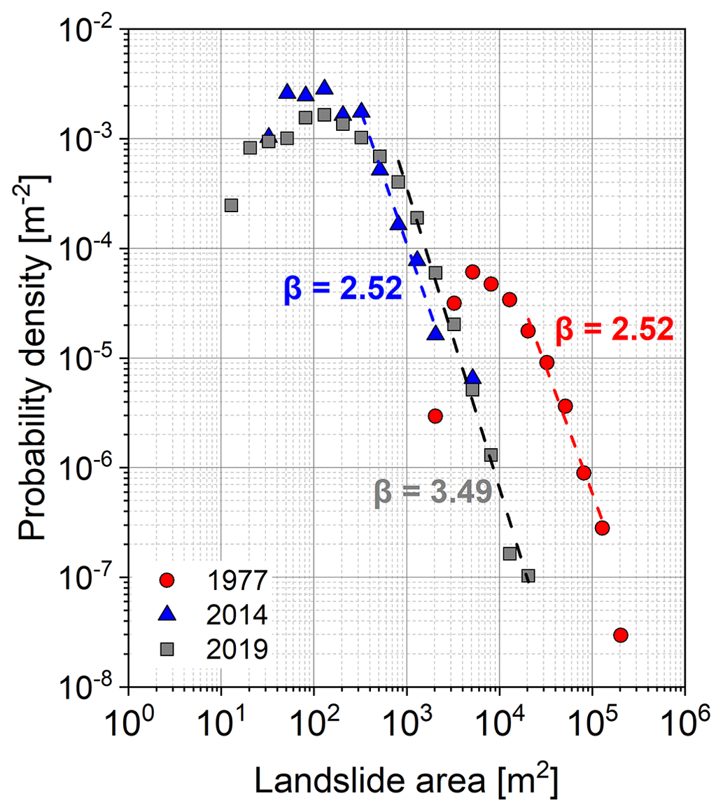
Figure 3 Probability density – areal distribution of the shallow landslides for the three events within the study area. As stated in the main text, the 1977 landslide inventory shows a different distribution, shifted to the right, because of the different chosen mapping criteria. Power-law fitting with the maximum likelihood estimator is reported ($\mathit{\beta }=-\mathit{\alpha }-\mathrm{1}$).

2.3 Slope unit delineation

The application of statistical models to landslide susceptibility zoning requires the partition of the study area in terrain units, such as unique condition units, slope units, grid cells, or others (Carrara et al., 1991, 2008). Among these, slope units were chosen for areal partitioning within this study. A slope unit is defined as a morphological terrain unit delimited by drainage and divide lines (Carrara et al., 1991; Guzzetti et al., 1999), corresponding to what could be defined as a single slope, a combination of adjacent slopes, or a small catchment from a geomorphological and a hydrological point of view (Alvioli et al., 2016). Slope units were selected since they provide several advantages, such as (i) the reproducibility of the spatial partitioning; (ii) the possibility to use continuous values for the categorical variables, where the continuous values are calculated as the areal percentage of the slope units that are covered by a particular categorical class and thus can vary between 0 % and 100 % (Carrara et al., 1991); and (iii) an efficient handling of mapping uncertainties, thanks to the generalization of the predisposing factors falling within them (Jacobs et al., 2020; Steger et al., 2016). Their delineation is based on the identification of drainage and divide lines and was done automatically by using the r.slopeunits algorithm (Alvioli et al., 2016). This iterative algorithm requires as input data the minimum circular variance for each unit, representing the allowed variability of orientation for each grid cell belonging to the same unit, and the minimum area for each slope unit.

2.4 Preliminary exploratory statistical analysis

To understand which variables exert the strongest control on the landslide distribution and if this control remains constant through time, the distributions of the mean values of each covariate for the slope units affected by shallow landslides were compared with the same distributions for the whole study area, as well as for the other inventories. The similarity among the inventories for each covariate (i.e. the null hypothesis) is rejected if the p value of Dunn's test is smaller than 0.05.

To further investigate the role of antecedent and triggering precipitation, the relationship between landslide density (i.e. total landslide area over the total slope units area) and precipitation classes (i.e. normalized maximum rainfall intensity, normalized cumulative rainfall, and normalized antecedent cumulative rainfall) was analysed through Spearman's rank order correlation coefficient. Given the strong lithological control, the analysis was conducted for the entire study area and separately for the most unstable lithological units.

2.5 Rainfall-based susceptibility analysis

Binary logistic regression was chosen for the susceptibility analysis because of its widespread and validated use and because it provides the importance of each conditioning variable in terms of standardized regression coefficients in a straightforward manner (Carrara, 1983; Micheletti et al., 2015; Reichenbach et al., 2018).

Logistic regression describes the relationship between a binary outcome (stable or unstable unit) and a set of independent variables (Hosmer and Lemeshow, 2000). The probability p of a sample to belong to a certain group is given by

$$\begin{array}{}\text{(3)}& \ln {\displaystyle \frac{p}{\mathrm{1}-p}}=B_{\mathrm{0}}+B_{\mathrm{1}}{X}_{\mathrm{1}}+B_{\mathrm{2}}{X}_{\mathrm{2}}+B_{\mathrm{3}}{X}_{\mathrm{3}}+\mathrm{\dots }+B_m{X}_m,\end{array}$$

where B_i represents the logistic coefficients, estimated from the data, that quantify the contribution of each variable X_i to the final outcome. Logistic regression assumes that a linear relationship exists between the logit transformation of the binary outcome and each variable selected by the model through a forward stepwise method, with a variable being included in the model if the probability of its score statistics is smaller than an entry value of 0.05 and being removed if the probability is greater than a removal value of 0.10. Before running the models, variables showing a strongly skewed distribution were normalized using a log-transformation (Carrara et al., 2008), and all the static variables were then standardized using a z-score normalization (mean equal to 0 and standard deviation equal to 1), in order to make their estimated regression coefficients comparable (Lombardo and Mai, 2018).

Five susceptibility models were developed. Models m77, m14, and m19 were trained on a single landslide event (i.e. 1977, 2014, and 2019, respectively). Model m771419 was trained by merging all the landslide events, and finally model m7714161921 was trained by merging different rainfall events with or without landslides. Each dataset was divided into training ($\mathrm{3}/\mathrm{4}$) and validation ($\mathrm{1}/\mathrm{4}$) subsets, the former being used to build the models and the latter to evaluate their predictive performance. Each model was evaluated against itself and against all the other landslide events by using cross-validation. Model evaluation was performed with the following strategy. First of all, two common cut-off-independent methods were applied (ROC and precision–recall–gain (PRG) curves) to obtain their area under the curve values (hereafter referred to as AUROC and AUPRG values). Then, the optimal cut-off obtained by the ROC analysis was used to derive the optimal contingency matrix, from which the accuracy, precision, TPR, and FPR were calculated.

Finally, the two values under the ROC and PRG curves and the four performance metrics calculated from the contingency matrix were summed up with a multiple attribute decision-making procedure, performed with the technique for order preference by similarity to ideal solution (TOPSIS; Hwang and Yoon, 1981) to individuate the best model. For each model, 50 logistic regression analyses were run with different training and validation datasets, randomly extracted from the original database. This procedure lead to the calculation of 50 different values of the coefficient associated with each controlling variable and to the generation of 50 different susceptibility maps, thus allowing us to statistically analyse the distribution of the susceptibility values, the regression coefficients, and the performance metrics.

To avoid an overabundance of obviously stable units (e.g. flat areas), which would give a biased estimate of the performance, only nontrivial units with slopes more compatible with shallow landslides triggering (>20° and < than 40°) were selected.

The economic consequences are one of the main issues in early warning; these economic costs can be significantly different in the case of false or missing alarms. This problem is usually not considered in susceptibility studies, where the classification of susceptibility into classes (e.g. very low, low, medium, high, and very high) is based on some arbitrary choice of the modeller (Cantarino et al., 2019).

For this reason, a new practical approach to classify the susceptibility values was defined, based on the cost–curves approach. Similarly to other methods, such as “natural breaks” (Jenks, 1967), this procedure takes into account the underlying data instead of using standard classes, with the advantage that it can be calibrated on a specific cost analysis.

Specifically, the cut-off corresponding to the minimum normalized expected cost was used as the centre of the third class (medium susceptibility) and defined in this work as the half-susceptibility threshold (HST). The class limits are defined based on a geometric progression from 0 to 1, centred on HST.

Since the misclassification costs can vary significantly within the study area and since their quantification require extremely detailed analyses, in the current work the a priori probabilities of having and not having landslides were kept equal, while three scenarios of relative costs were considered (Scenario 1 with $c\left(-|+\right):c\left(+|-\right)=\mathrm{0.5}:\mathrm{0.5}$, Scenario 2 with $c\left(-|+\right):c\left(+|-\right)=\mathrm{0.8}:\mathrm{0.2}$, and Scenario 3 with $c\left(-|+\right):c\left(+|-\right)=\mathrm{0.2}:\mathrm{0.8}$, where $c\left(-|+\right)$ is the cost of false negatives and where $c\left(+|-\right)$ is the cost of false positives).

3 Results

3.1 Slope units delineation

By using a minimum area of 20 000 m² and a maximum circular variance of 0.1, the study area was partitioned into 10 528 slope units (Fig. 4), with an average area of 56 555 m² and a maximum area of 1 868 299 m². Slope units were classified as unstable if occupied by at least one landslide. This resulted in 627 (5.95 %), 50 (0.47 %), and 869 (8.25 %) unstable slope units for the 1977, 2014, and 2019 events, respectively.

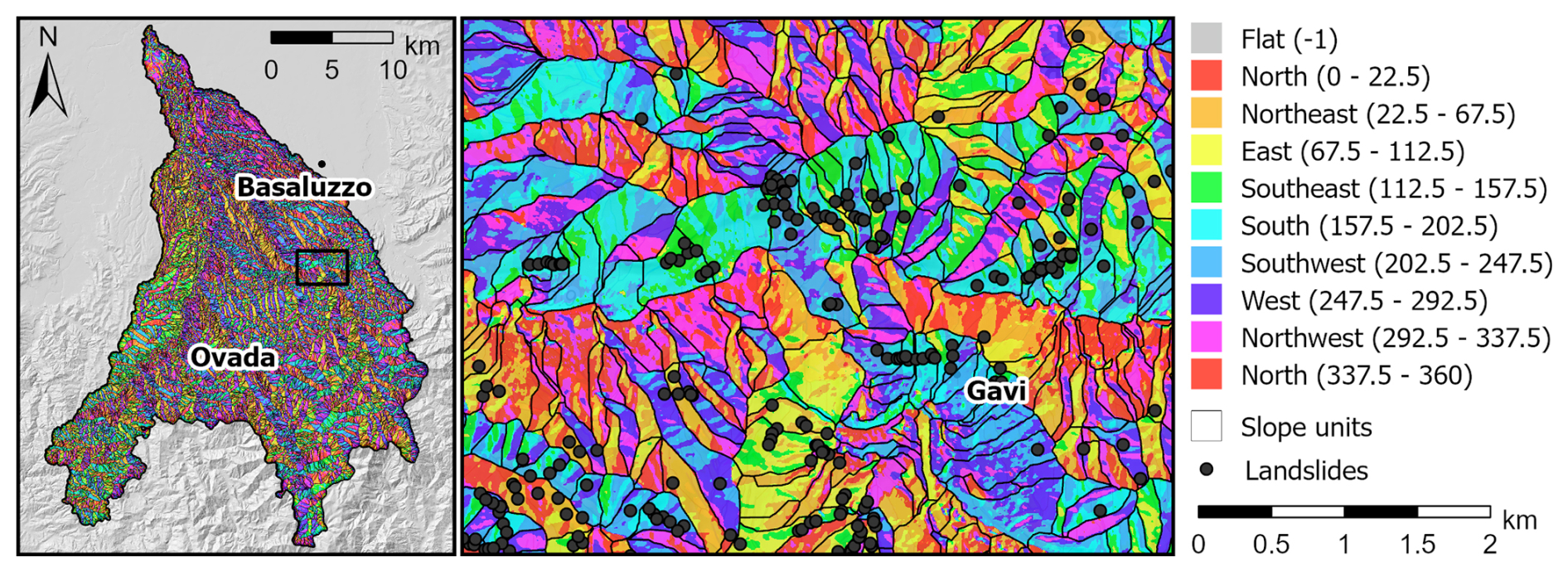
Figure 4 Example of slope unit delineation within the area of Gavi, overlaid on an aspect map.

3.2 Preliminary exploratory statistical analysis

Figure 5 represents the percentage of variables within the different groups of controlling factors for which the similarity hypothesis between the variable distributions in the unstable slope units for the different inventories can be rejected (see Fig. S5 for all the distributions). Lithological variables show the lowest dissimilarity between the different inventories, followed by land use. On the other hand, the rainfall variables are always dissimilar among the inventories. This suggests that landslides may be triggered by different rainfall patterns but within certain specific lithological and land-use classes.

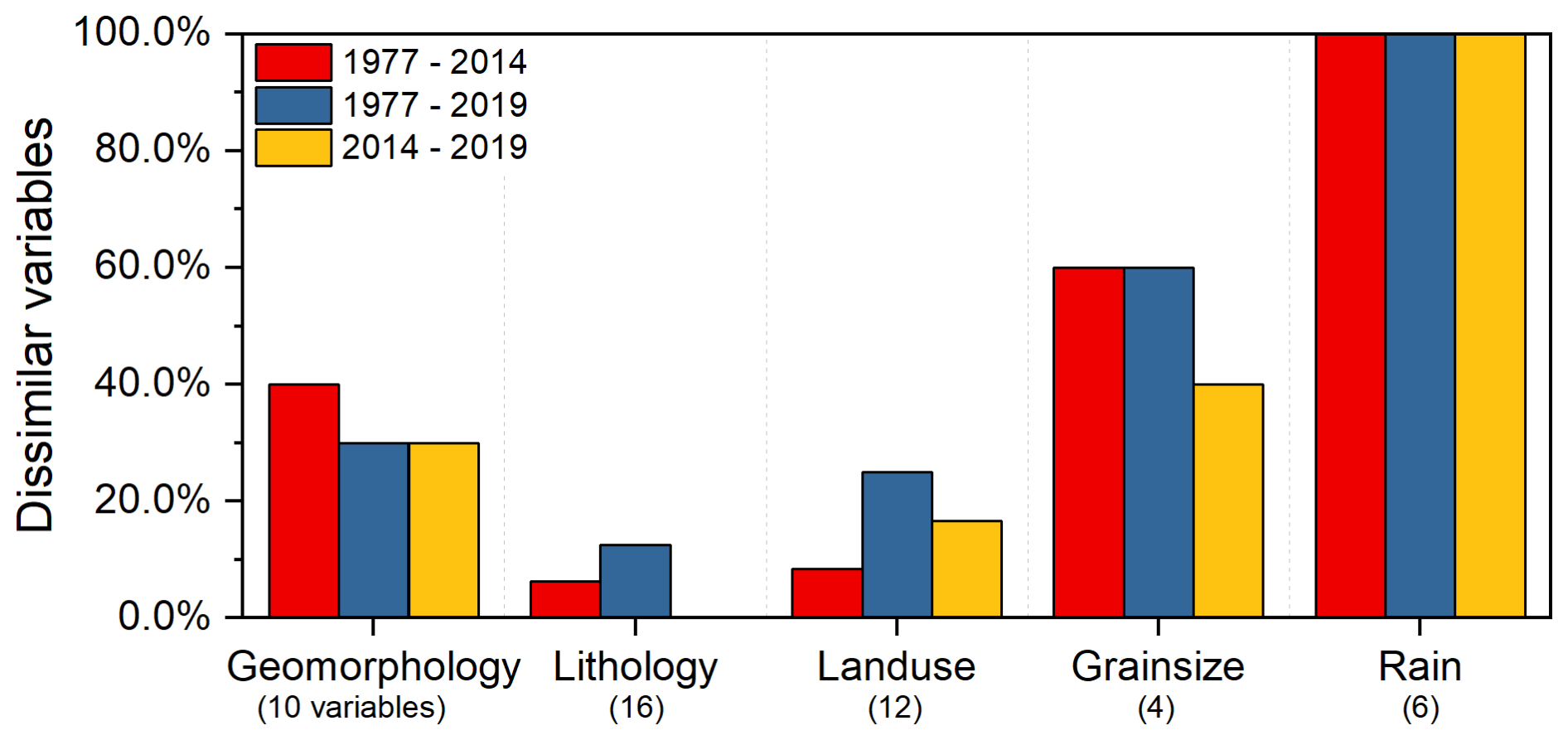
Figure 5 Percentage of statistically dissimilar variables within each group of controlling factors, according to Dunn's test with a significance level of 0.05. Numbers below the name of the groups refer to the total number of variables considered within that group.

To further investigate the control exerted by rainfall on the triggering of shallow landslides, the correlation between landslide distribution and values of maximum rainfall intensity and 90 d antecedent cumulative rainfall was analysed. This investigation was carried out by defining intervals of rainfall values and calculating the spatial density of landslides within each rainfall interval area. The three landslide events show significant differences, confirming the previous results. Considering the whole study area, landslide density is clearly positively correlated with maximum rainfall intensity. For the same maximum rainfall intensity values (Fig. 6a), the landslide density is offset for the three inventories, suggesting a different sensitivity of landslides to rainfall (e.g. landslide density for 400 mm is $\mathrm{4.36}\times {\mathrm{10}}^{-\mathrm{4}}$ for the 2014 event and $\mathrm{4.65}\times {\mathrm{10}}^{-\mathrm{3}}$ for 2019). This could be explained by the different levels of antecedent rainfall (Fig. 6b): the higher the antecedent cumulative rainfall, the higher the sensitivity. This relationship is also recognizable by visual comparison of the event rainfall intensity maps with respect to the antecedent cumulative rainfall maps (Figs. 2 and S2).

The same analysis was conducted for the most unstable lithological units, namely marls (around 30 % of the total landslides number for each event), sandstones and siltstones (almost 50 % of landslide in each event), sandstone breccias (7 % of landslides in 1977 and 2019, 0 % in 2014), and sandstones and marls (4 % in 1977 and 2019, 14 % in 2014). The results did not show clear trends, probably due to the low number of landslides in each rainfall class (Fig. S6). This is more evident for sandstone breccias, as this lithology is restricted to a relatively small sector in the western part of the study area.

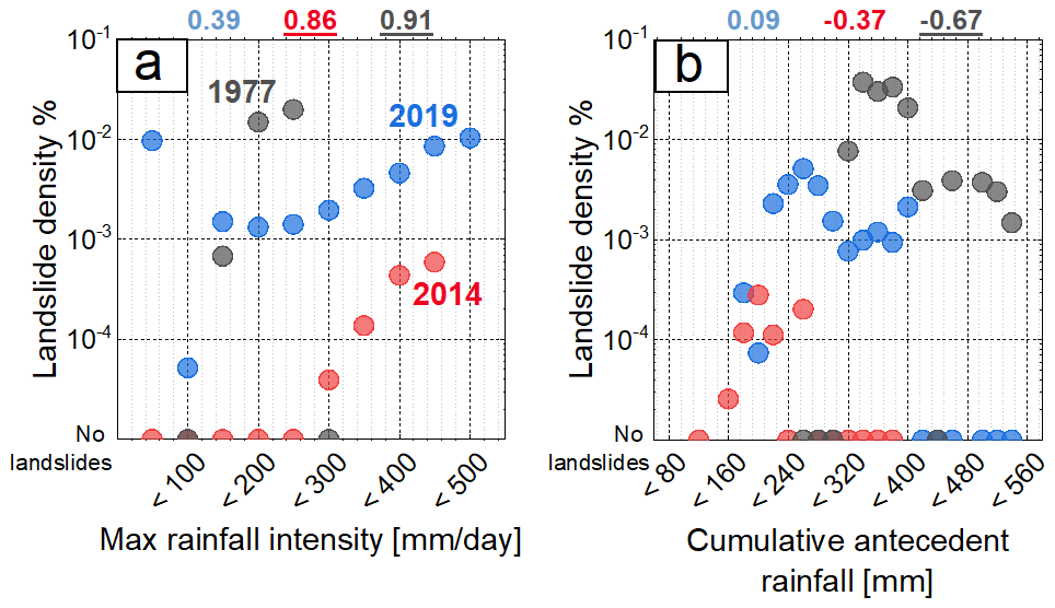
Figure 6 Scatterplots representing landslide density in each rainfall class (spanning 50 mm of rainfall in 24 h and 20 mm of antecedent cumulative rainfall) for the entire study area. Spearman's rank order correlation coefficients between landslide density and rainfall classes are reported in each plot. Underlined values are statistically correlated at the 0.05 level.

For the 1977 event, Fig. 6a shows that landslides started to occur for maximum rainfall intensities greater than 100 mm in 24 h. This result agrees with the intensity–duration (ID) threshold curves proposed for the area (Tiranti et al., 2019). A few landslides in 2019 were triggered at even lower rainfall values, very close to the catchment divide where local topography could have exerted a major control. The high density is also related to the small catchment area pertaining to the low rainfall interval. On the other hand, during the 2014 event, a rainfall intensity of 250 mm in 24 h was necessary to cause instabilities. This may be explained by a relatively low cumulative antecedent rainfall (below 300 mm) with respect to the other events, inducing low initial soil moisture conditions.

3.3 Rainfall based susceptibility maps

Figure 7 shows the mean coefficient and the inclusion rate of the 50 runs of the logistic regression models for each single variable. Slope gradient is the most important parameter for all models (except m14), with always positive coefficients and a high inclusion rate. For the other morphometric parameters, northernness and flow accumulation show a high inclusion rate and relatively high coefficients (except for m14). The negative sign of the northernness coefficient indicates the south-facing slope units as more unstable. Among the lithological descriptors, “gravels and sands”, “sandstones and siltites”, and “marls” show the highest inclusion rates and coefficient values. On the other hand, basalts, limestones, and slates are never included in the models. Land use does not exert an important control. Among the descriptors of soil granulometry, the contents in coarse fragments and sand are selected with a high inclusion rate and a negative median coefficient, with the exception of m14, while clay content is chosen with a high inclusion rate and a positive median coefficient.

Eventually, rainfall variables play an important but complex role in susceptibility. Maximum daily intensity is very important for m14, m771419, and m7714161921, with positive coefficients and a high inclusion rate. Surprisingly, maximum rainfall intensity is not included in m19 and takes negative values in m77. The antecedent cumulative rainfall is important for slope instability in models m77, m14, m771419, and m7714161921, while model m19 shows the lowest mean coefficient for this variable.

The intra-event maximum rainfall intensity is also a relevant variable but with a more complex influence. This variable is very important for model m14, with a strong destabilizing effect, but it is not included in model m19 and assumes a negative coefficient in m77.

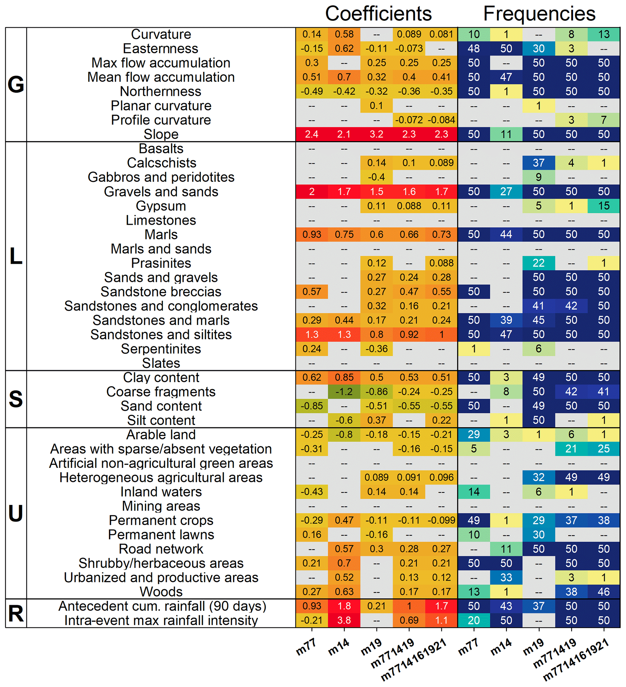
Figure 7 Variation of the median coefficient (left panel) and inclusion rate (frequency – right panel) of variable selection according to the different training models, based on 50 iterations. Variables are aggregated into five groups (G = geomorphological parameters, L = lithological parameters, S = soil grain size, U = land use and land cover parameters, R = rainfall parameters). Grey boxes indicate that the variable was never chosen by the model.

Model m14 shows a good performance when evaluated over its validation dataset, with a mean AUROC value of 0.97 (highest mean AUROC value among all the tested models), but it fails in predicting or hindcasting other landslide events, as indicated by an interquartile range of AUROC values between 0.62 and 0.74 (Fig. S7), a low accuracy, and a high FPR. Model m77 shows a high mean AUROC but a low AUPRG, especially when trying to predict 2014 landslides, meaning that the model output becomes less precise when ignoring the true negatives. On average, model m19 shows good prediction capabilities, especially in terms of AUPRG. Models trained over multiple events show the best performance and an associated reduction in the variability of the final results. The mean AUROC value increases, as does the mean AUPRG. The inclusion of intense rainfall events that did not lead to the triggering of slope instabilities results in small improvements in the general performance, especially for the mean accuracy and FPR.

According to the TOPSIS classifier (Fig. 8), m7714161921 is the model with the highest relative closeness degree to the ideal solution (score of 0.9), obtained giving the same weight for the evaluation of all the scores (0.16 for all the metrics).

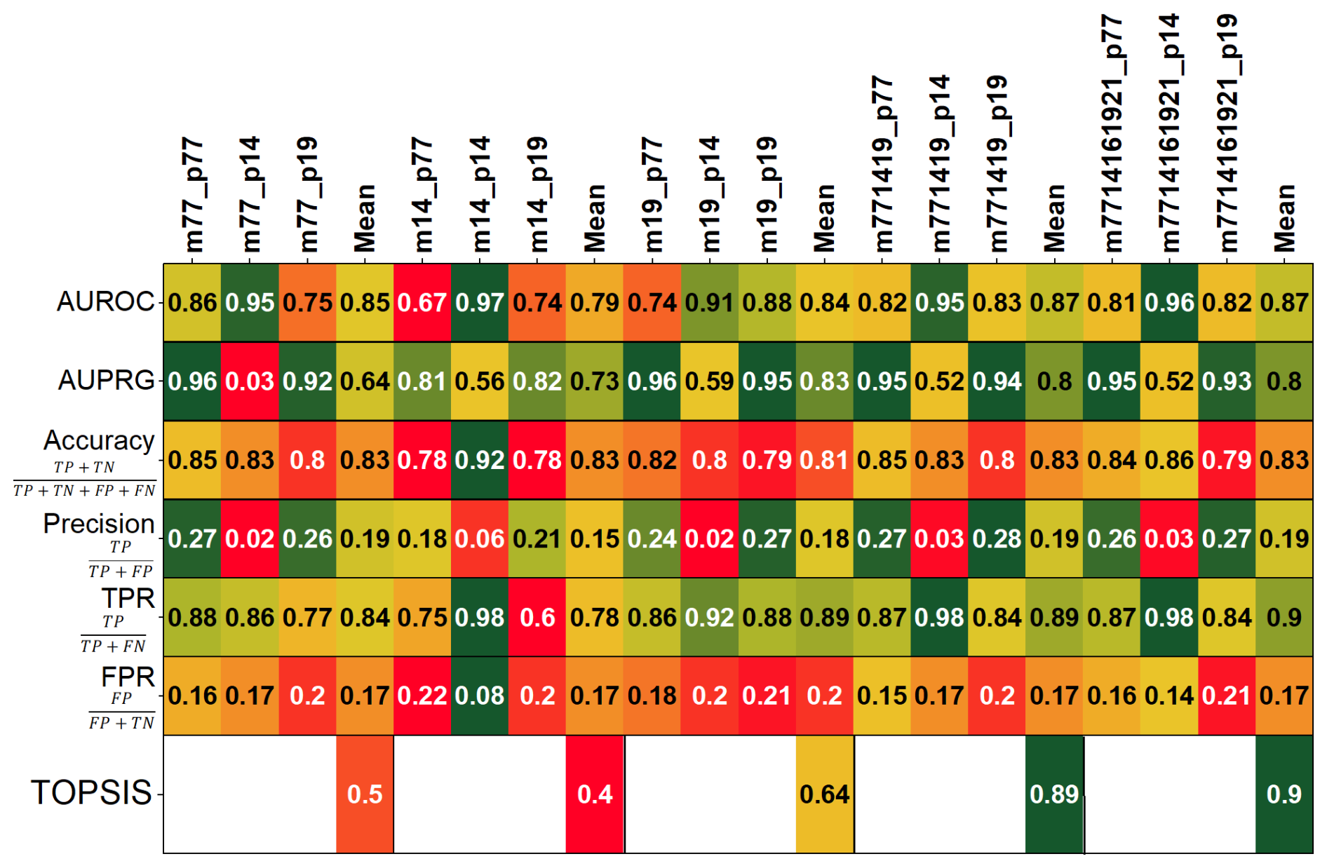
Figure 8 AUROC, accuracy, precision, true positive rate (TPR), and false positive rate (FPR) obtained using the threshold that minimizes the expected costs, calculated for each model assuming equal costs. For each model, the scores of the evaluation obtained with the TOPSIS classifier are also reported.

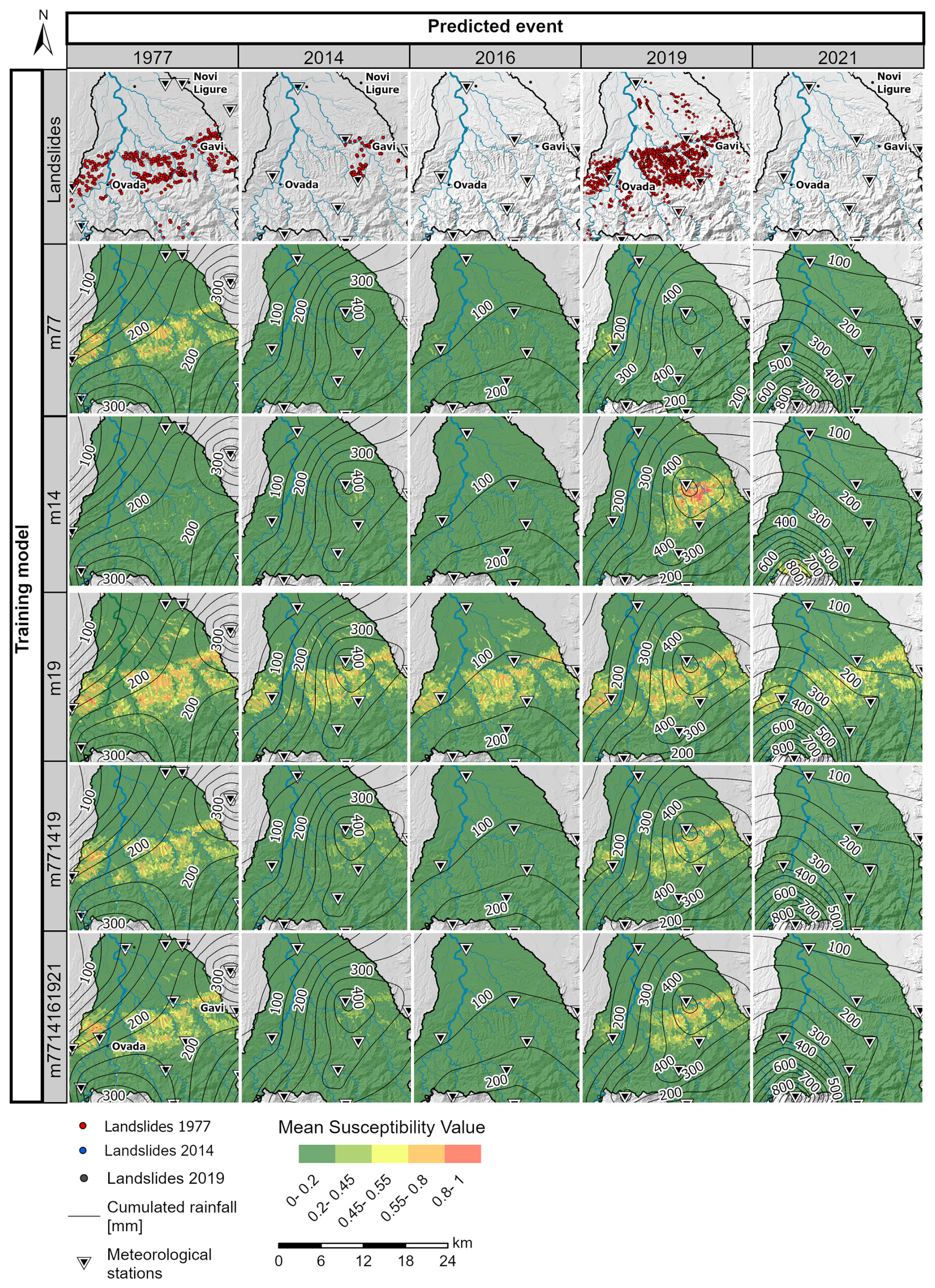
Figure 9 Landslide susceptibility maps for the Orba basin. Columns refer to different training models, while rows refer to different predicted or hindcasted events.

3.4 Model representation

For each model, five rainfall events were used to produce the rainfall-based susceptibility maps (Fig. 9), obtaining different maps for each model as a function of the event-specific rainfall values. From a simple visual inspection, comparing susceptibility classes and landslide distribution, it is clear that models m14 and m19 are not able to correctly model landslide susceptibility. As already seen in Fig. 7, the high coefficient of rainfall intensity in m14 makes susceptibility excessively dependent on this variable, so the resulting unstable units simply reflect its distribution. On the contrary, the exclusion of rainfall intensity and the low coefficients of antecedent rainfall in m19 make the susceptibility maps almost constant for different events. In addition, the model tends to overestimate unstable areas. Model m77 shows a better performance but still suffers from the low coefficient of maximum rainfall intensity, making this model also quite constant between different events, thus also predicting unstable areas for the 2016 and 2021 events. Models m771419 and m7714161921 significantly outperform the others, as they are able to classify the central part of the study area as unstable only for heavy rainfall events. However, they tend to underestimate the percentage of unstable or very unstable slope units during the 1977, 2014, and 2019 events, with less than 4 % of the slope units classified as moderately, highly, or very highly unstable. On the other hand, they correctly classify all the slope units as stable when considering rainfall events that were not associated with landslides (p16 and p21). Model m7714161921 also shows a slightly better ability to handle false positives when simulating non-triggering rainfall events, as can be seen in the last row of Fig. 7 for the prediction of m14, m16, and m21, especially in the western part of the study area.

In general, the maps in Fig. 9 classified by using a rather standard partitioning of the susceptibility values into five classes (0–0.2, 0.2–0.45, 0.45–0.55, 0.55–0.8, 0.8–1) show an uneven distribution of slope units in the different classes, giving the impression of either overestimation or underestimation. This problem was addressed with the new classification method based on misclassification costs, which was applied to m7714161921 (ranked as the best-performing model). For each of the three considered scenarios, the optimal cut-off threshold and the relative geometric progression were derived, considering different misclassification cost ratios (Table 2). The class boundaries derived from the geometric progression were then used to reclassify the susceptibility values to produce optimized maps (Fig. 10). The optimal cut-off threshold decreases as the relative cost of false negatives decreases, thus reducing the number of slope units classified as unstable.

Table 2 Threshold values for m7714161921 for each of the proposed scenarios of relative costs. HST is the half-susceptibility threshold corresponding to the value that minimizes the normalized expected cost for each cost scenario. The considered classes correspond to very low (VL), low (L), medium (M), high (H), and very high (VH).

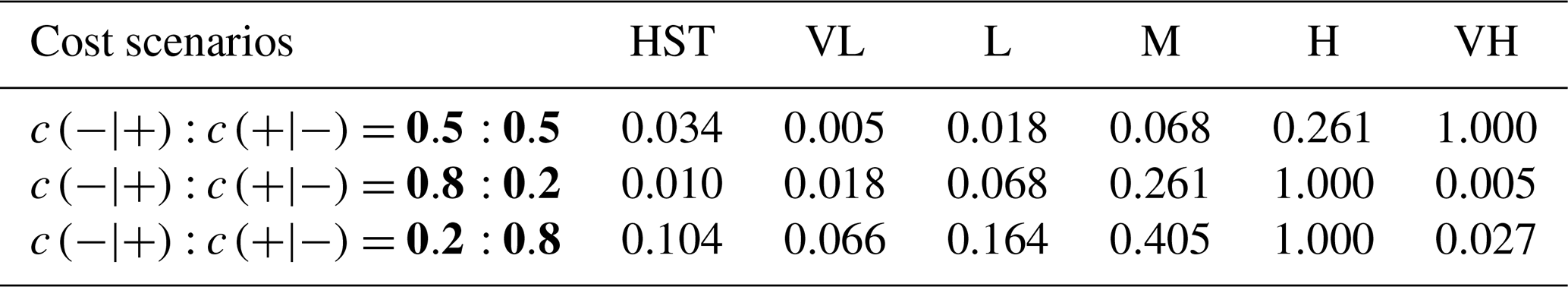
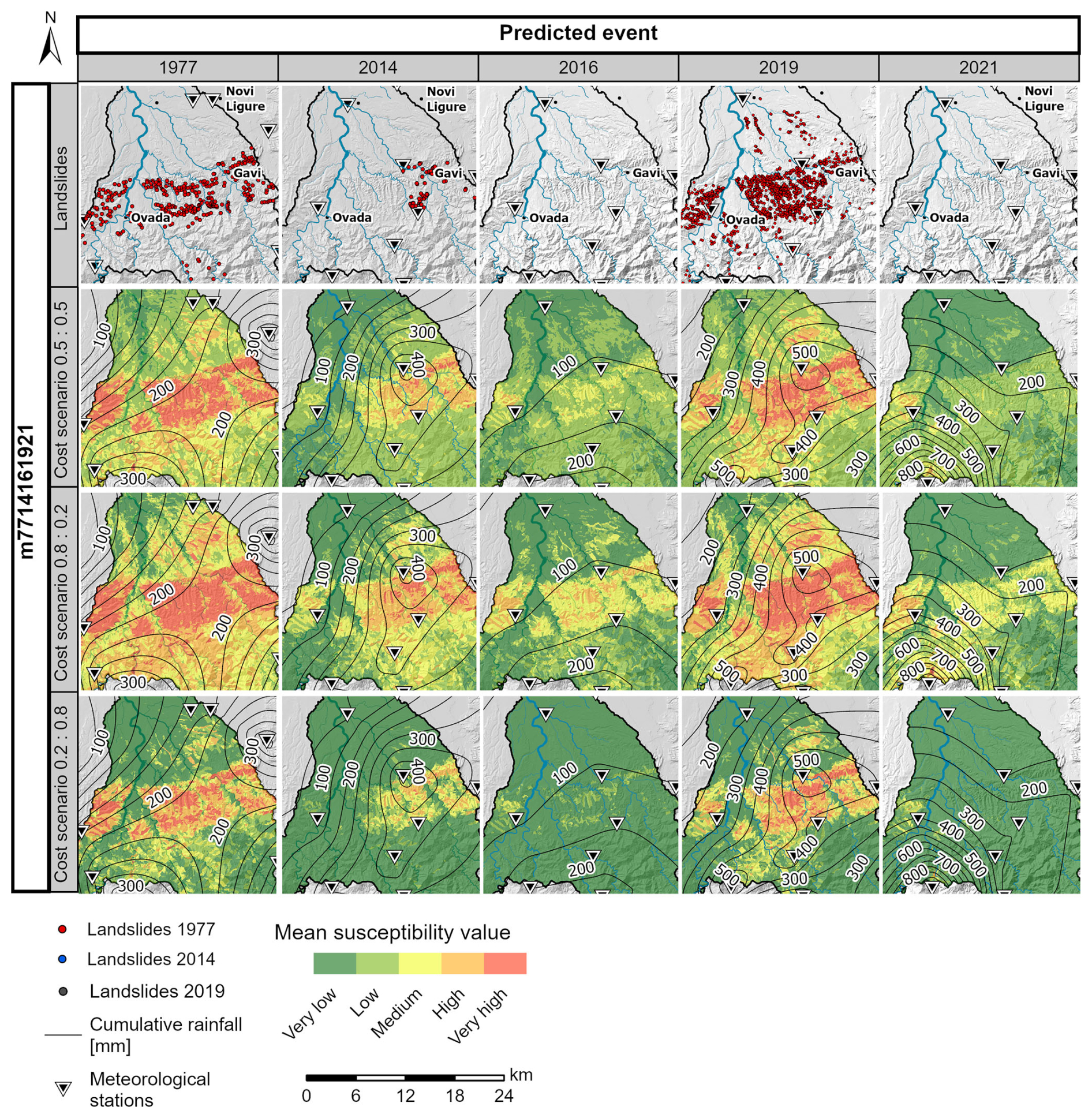
Figure 10 Instability maps relative to the best-performing model (m7714161921). Each row refers to a different relative cost scenario, where the proportions refer to the ratio between costs associated to false negatives and false positives. Class limits are defined based on the optimal cut-off threshold and the relative geometric progression.

4 Discussion

4.1 Landslide distribution analysis and prediction

This paper investigated the relationship between several spatially distributed variables (i.e. possible triggering factors) and the occurrence of shallow landslides though a logistic regression-based susceptibility analysis.

At a first visual inspection, the spatial distribution of the shallow landslides is fairly constant in all the available inventories, suggesting that shallow landslides in this area are modulated by rainfall but controlled by other static parameters. In particular, landslides tend to occur in slope units with similar geomorphology and lithology (Fig. 5).

More specifically, besides the slope gradient, lithology appears to be the most important variable that controls landslide susceptibility (Fig. 7). Among all, the most prone lithologies in all the inventories are marls, sandstones, and siltites, similarly to the results of Luino (1999) and Licata et al. (2023). The high importance given to gravels and sands, a lithology commonly found in alluvial flat areas, can be explained with the instability of fluvial terraces (Šilhán, 2022). Moreover, the lithology controls the grain size of the soil cover and, thus, the hydrological processes in the unsaturated zone. The sedimentary sequence in the central part of the area, overlaid by soils with a high clay content, is another important destabilizing factor in the model because of the poor draining capacity of clays. More interestingly, the southern metamorphic basement is commonly covered by soils rich in sand and coarse fragments, which have a strong stabilizing effect, probably correlated with a higher drainage capacity and friction angle.

Surprisingly, the role of land use does not appear to be relevant. In addition, the role of lithology may be strong enough to mask the land-use effect.

Looking at the variables related to rainfall dynamics, the cumulative antecedent rainfall is the most relevant in all regression models. In fact, it has been considered a proxy for the soil water content before the event, which for various authors it is pivotal for modelling shallow landslides (Bogaard and Greco, 2018; Marino et al., 2020). The intra-event maximum rainfall intensity is also a relevant variable, but with a more complex influence. Being calculated with a 24 h aggregation time, this variable can be intended as a general descriptor of the entire rainfall event, representative of both the rainfall intensity and the daily cumulative value. Using a smaller aggregation time could help to differentiate the effects of these two descriptors, which was impossible for the event of 1977, as outlined in Sect. 4.2.

These parameters are also important to explain the spatial distribution of the landslide density. In particular, the analysis of the relationships between landslide density, the normalized maximum rainfall intensity over 24 h, and the normalized values of the antecedent cumulative rainfall suggest that landslide density appears to be controlled by the maximum rainfall intensity. This agrees with the mechanical explanation of shallow landslide triggering, controlled by soil saturation, leading to an increase in pore pressure and a loss of soil suction (Fredlund et al., 1978). In addition, the antecedent condition shows a double role of setting a threshold required for landslide initiation (e.g. Crozier, 1999; Glade et al., 2000; Godt et al., 2006; Marino et al., 2020b) and offsetting the relationship between landslide density and rainfall intensity.

Several basin-scale studies suggest that to quantify the shallow landslide susceptibility the use of multi-temporal inventories leads to better results (Reichenbach et al., 2018), while others affirm that this is not always associated with a model performance improvement (Ozturk et al., 2021; Smith et al., 2021). Results show that, for the Orba basin, models trained over a single landslide event are not capable of catching the real processes underlying the instability phenomena, despite the high landslide density and the good performance when using the validation dataset. Thus, they are unable to predict landslide events associated with different rainfall characteristics. In particular, m14, being the smaller landslide inventory and more limited in the extend of the affected area, shows the best performance when tested against itself (Figs. 8 and S7) and the worst performance when used to model other events, producing maps with an exaggerated landslide susceptibility in areas with high precipitation. The inclusion of multiple events helps in stabilizing the effect exerted by the different controlling variables, thus providing more reliable prediction/hindcast susceptibility maps.

The evaluation of the performance of regression models is always challenging, especially when using an input dataset with a skewed distribution (e.g. Provost et al., 1998; Davis and Goadrich, 2006; Drummond and Holte, 2006). AUROC, which is the most used evaluation method in the literature (Reichenbach et al., 2018), suffers from an overly optimistic evaluation while misclassifying the samples that belong to the underrepresented class. This is the case for model m77 when predicting the 2014 event. On the other hand, AUPRG shows high values when model m77 predicts the 2019 event, even if large parts of the area affected by landslides are predicted as stable. The other indices are cut-off dependent, and they do not show any capabilities to discriminate among the different models. For these reasons, the multi-criteria TOPSIS model was used to consider the contribution of all the indices. Based on the TOPSIS evaluation, the multi-temporal models outperform the single-event models, confirming what was discussed above. In particular, the model with the highest prediction capabilities is m7714161921, suggesting that the inclusion of non-triggering rainfall events helps in defining the rainfall threshold to trigger instabilities in different parts of the study area.

For the representation of the results, the classification scheme typically adopted in the literature does not account for misclassification costs (Cantarino et al., 2019), meaning that the costs associated with false and missed alarms are implicitly assumed equal. However, since the misclassifications costs are often not equal, the total misclassification cost can be reduced by playing on the degree of conservativeness of the models in order to reduce the false negative or false positive rates, thus increasing or decreasing what is classified as unstable. This required a new classification scheme to adjust the thresholds used for susceptibility classification according to the selected proportion of misclassification costs.

Scenario 2, where the costs of false negatives are higher, is the most conservative, because the classification is forced towards instability to keep the false negative rate low. On the contrary, scenario 3, where the costs of false positives are higher, shows the highest percentage of stable slope units. Scenario 1 considers equal costs for false positives and false negatives, and it produces intermediate results. The strong differences between these scenarios suggest that the use of cost curves for the landslide susceptibility model could be a valuable tool in the final stages of a susceptibility analysis, when slope units need to be classified. This approach allows for different classification thresholds based on cost combinations, enabling the evaluation of their consequences. Costs may include direct costs like damage to infrastructure and loss of life and indirect costs like traffic disruptions and lost productivity (Sala et al., 2021). While this work uses different cost ratio scenarios to demonstrate the approach's potential, more detailed analyses could provide precise cost quantifications, considering that costs may vary across different parts of the study area.

4.2 Challenges, uncertainties, and limitations

It is necessary to underline possible uncertainties and assumptions regarding the input datasets and the modelling strategies so that the limitations of our findings are made clear. Two main limitations can potentially affect the results of these analyses: the consideration of land use and land cover as a static variable and the use of an old landslide inventory.

First, land use and land cover can vary greatly over time. Considering this variable as static is mainly due to a lack of information, since the only other dataset provided by ARPA Piemonte dates to 2010, and the analysis of satellite images, besides being beyond the purpose of this study, was not possible for the 1977 event. An analysis of the land-use change between two available datasets (2010 and 2021) within the Orba basin revealed that permanent crops decreased by 6 % and meadows by almost 2 %, while the areas characterized by shrub and herbaceous vegetation increased by 4 % and the woods by almost 4 %. However, these changes can be considered negligible in the analyses, given the very low influence of the land use variables in the logistic regression. This is in contrast with the conclusions of many other studies (e.g. Bernardie et al., 2017; Persichillo et al., 2017; Hürlimann et al., 2022), suggesting that this relationship could be further analysed in future studies.

The second limitation is posed by the inclusion of an older event (1977) with higher uncertainty of both rainfall pattern and landslide distribution. Data from the ARPA Piemonte and ARPA Liguria weather stations were used to analyse the rainfall pattern. However, only 36 stations were active in 1977, 26 % less than in 2014 and 2019, and most of them are located outside the region of interest (Fig. 2). This uncertainty in the rainfall pattern could affect the modelling, especially in the central part of the basin. In addition, data for 1977 were only available with a daily time step, making it impossible to use multiple different aggregation times. The landslide inventory of the 1977 event represents landslides as areas affected by diffuse shallow landslides rather than individual polygons. This affects the landslide distribution and density analysis. However, the choice to use slope units for analysis mitigated this difference in the inventories. Finally, as mentioned above, the use of this landslide event precluded the use of satellite products; therefore, some factors that could improve susceptibility analyses, such as satellite-based antecedent soil moisture, could not be incorporated into the model.

5 Conclusions

This study demonstrates the feasibility of using logistic regression to model the effects of extreme rainfall events on the stability of a complex study area, such as the Orba basin in the Piedmont region of Italy. In this area, the spatial distribution of shallow landslides reflects the distribution of lithology and geomorphology, thus showing a similar pattern for different rainfall scenarios.

In such conditions, the development of a rainfall-dependent model capable of simulating different susceptibility scenarios is more challenging and requires a careful calibration of the model with representative and significant rainfall events over a multi-temporal dataset. In fact, the use of single events may be problematic. For example, a rainfall event that is spatially concentrated in a small area with specific geological characteristics (such as in 2019 for the study area) could overestimate the role of such characteristics despite the rainfall, producing biased scenarios. On the contrary, a model trained on an extreme localized event spanning different geological conditions (such as the 2014 event) may overestimate the role of rainfall at the expense of geology. Finally, a rainfall event evenly distributed over the area (such as in 1977) would produce a model that underestimates the role of rainfall in controlling the landslide pattern.

To avoid such effects, an ensemble of rainfall events is preferable to better unravel the effects of the triggering variables and also to compensate for local misleading effects that may arise from the use of a single rainfall event. The use of rainfall events that did not trigger landslides may also be helpful for such compensation. The proposed strategy for selecting the best ensemble of rainfall events was based on the maximization of the AUROC, AUPRG, accuracy, and precision, as well as the minimization of the expected misclassification costs.

Eventually, misclassification costs were adopted as a criterion to define the susceptibility classes for the practical use of the resulting maps; this highlights the need to give importance to the classification process, which should be tailored to the needs of the end users and for the purpose of the final products.