the Creative Commons Attribution 4.0 License.
the Creative Commons Attribution 4.0 License.
 | 07 Nov 2025
Machine learning for automated avalanche terrain exposure scale (ATES) classification
Andreas Huber
Momchil Panayotov
Christoph Hesselbach
Paula Spannring
Jan-Thomas Fischer
Michaela Teich
Avalanche risk management is essential for backcountry safety. The Avalanche Terrain Exposure Scale (ATES) classifies mountain terrain based on its potential exposure to avalanche hazards and supports mountain visitors in their terrain assessment. Initially, ATES maps were generated manually, a costly and time-consuming process. Automated ATES model chains (AutoATES) have been developed to address these limitations, but existing approaches require careful parametrisation when applied to novel areas.
This study applies machine learning methods, specifically Random Forests, for automated ATES classification by replacing expert-driven AutoATES classification trees with a data-driven approach. Using a labelled training dataset from the Pirin Mountains, Bulgaria, we trained and evaluated three Random Forest models to assess their potential in classifying avalanche terrain. We analysed the influence of various input features, including slope, potential release areas, and percent canopy cover, on classification performance. Our results indicate that Random Forests offer a robust and scalable method for ATES mapping and that incorporating additional input features can improve classification performance. The accuracies for our Random Forest models on a held-out test set were 79.31 %, 82.32 %, and 80.42 %, demonstrating their potential for automated avalanche terrain classification and supporting safer backcountry decision-making.
- Article
(22617 KB) - Full-text XML
- BibTeX
- EndNote


Globally, snow avalanches cause an estimated 250 fatalities each year (Acharya et al., 2023; Schweizer et al., 2015), with more than one third of annual fatalities occurring on average in the European Alps (Techel et al., 2016). The amount of non-fatal incidents significantly exceeds these numbers. A large proportion of fatal avalanche accidents involves people recreating in the mountains, particularly skiers and snowboarders, often triggering the avalanches themselves (Schweizer and Lüschg, 2001; Techel and Zweifel, 2013; Engeset et al., 2018). These numbers clearly highlight the importance of supporting recreationists' decision-making in avalanche terrain by raising awareness, enhancing education, and providing information on avalanche terrain and current conditions (Toft et al., 2024).
In Bulgaria, backcountry skiing and snowboarding have seen a notable increase in popularity in recent years. Unfortunately, this increase has been accompanied by a growing number of avalanche-related incidents (Panayotov et al., 2021). Despite these developments, there is still limited information available to the public regarding current snowpack stability and avalanche danger or the spatial distribution of avalanche-prone terrain. Unlike in most Alpine countries no government-supported avalanche forecast exists. The only available forecast is provided by a non-governmental organization (Bulgarian Avalanche Association), and is limited to the Bansko Ski Resort area (Panayotov et al., 2024b). As a result, backcountry recreationists must rely primarily on their own judgment when evaluating current avalanche danger and navigating potential avalanche terrain. Therefore, there is a pressing need for clear and accessible information to enhance public awareness of avalanche-prone terrain and current snowpack stability, especially aimed at backcountry users with limited avalanche education and experience in terrain assessment and management (Panayotov et al., 2021). Similar gaps in publicly available avalanche information exist across many other mountain regions in the Balkan Peninsula and worldwide.
A simple and effective method for mapping avalanche-prone terrain and communicating it to backcountry users is the Avalanche Terrain Exposure Scale (ATES). Originally introduced by Statham et al. (2006) as a visitor management tool for national parks in Canada, ATES was developed to assess and convey the inherent avalanche risk of snow-covered mountainous terrain. Unlike avalanche forecasts, which provide dynamic assessments of current snowpack stability and avalanche danger, ATES offers a static classification that reflects the terrain's inherent avalanche hazard potential, independent of current snow or weather conditions. The initial version categorised terrain into three classes – simple, challenging, and complex (Statham et al., 2006). A later revision expanded the system to five classes, adding an extreme category and a designation for non-avalanche terrain (Statham and Campbell, 2025).
The ATES framework has been applied to map linear terrain routes (Parks Canada Agency, 2017) as well as to create comprehensive spatial maps. The first of these were developed by expert-based manual delineation. Examples include the mapping of more than 8000 km2 of avalanche terrain in western Canada (Campbell and Gould, 2013) or the production of ATES maps for a part of the Central Pyrenees (Gavaldã et al., 2013). In Bulgaria, geospatial technologies were first employed for avalanche terrain hazard mapping by Markov and Ivanov (2021), while the country's first ATES maps were also produced through expert assessment and manual GIS-based classification of an area near Bansko Ski Resort (Panayotov et al., 2021).
In recent years, significant efforts have been dedicated to developing automated procedures for generating ATES maps (e.g. AutoATES, Larsen et al., 2020) or similar avalanche terrain classification approaches (Schmudlach and Köhler, 2016; Harvey et al., 2018, 2024). The first iteration of AutoATES was introduced in Norway by Larsen et al. (2020), outlining a structured methodology consisting of three key steps: (1) identifying potential avalanche release areas (PRAs), (2) modelling their potential runouts, and (3) integrating this information into a final ATES map using a deterministic, decision tree-based classification scheme. The approach thus combines general physical understanding of the underlying processes with empirically-motivated models of avalanche release and runout, complemented by region-specific expert knowledge. A major limitation of the initial version was that it did not account for the influence of forest cover on potential avalanche hazard. Schumacher et al. (2022) demonstrated that incorporating forest data can substantially enhance the accuracy of ATES classification compared to approaches that omit this information.
To address this shortcoming and improve the general classification procedure, AutoATES 2.0 was developed by Toft et al. (2024), incorporating forest cover data to account for its protective effect against avalanches. AutoATES version 2.0 made use of ATES 2.0 (Statham and Campbell, 2025), which adds the extreme and non-avalanche terrain classes. Additionally, this version leveraged the open-source software Flow-Py (D'Amboise et al., 2022) to enhance avalanche intensity and runout modelling. AutoATES 2.0 has since been applied to different mountainous regions worldwide. For instance, von Avis et al. (2023) employed AutoATES to map avalanche terrain in the continental United States, while Huber et al. (2023) used a modified version to assess avalanche exposure in the Austrian Alps (AutoATES Austria).
The first use of automated ATES mapping in Bulgaria was carried out by Markov and Panayotov (2024), who based their work on the AutoATES 2.0 workflow. Subsequently, the methodology outlined in AutoATES Austria was applied to generate updated ATES maps for three test regions. While this approach proved effective in open alpine environments above the treeline, it faced challenges in accurately delineating avalanche terrain within forested areas, necessitating modifications of the expert-driven ATES classification tree and improvements to the input data, such as the creation of new algorithms to more precisely estimate forest percent canopy cover (Panayotov et al., 2024b). Furthermore, AutoATES relies on numerous thresholds and parameters, which must be carefully chosen and adjusted to local conditions. Identifying the optimal set of input features and thresholds for the classification is highly dependent on the specific characteristics of the terrain. As a result, expert knowledge is required to fine-tune all aspects of AutoATES, including PRA identification, runout approximation, and the final expert-driven ATES classification tree (Hesselbach, 2023). A method for optimising parameters in the AutoATES classification step by reverse engineering human ATES maps was recently proposed by Sykes et al. (2024), highlighting the importance of refining threshold values for local conditions.
Applying the AutoATES procedure to novel mountain areas requires in-depth understanding of the AutoATES model chain itself as well as intimate knowledge of the mountainous terrain being analyzed. This process can be challenging and time-consuming, as it demands a deep understanding of avalanche dynamics and the intricate dependencies between input parameters. Given these challenges, an ideal approach would be to create an automated ATES mapping procedure that integrates expert knowledge on local terrain and mountain characteristics, without having to rely heavily on manual parameter tuning and threshold adjustments in the AutoATES procedure.
Machine learning (ML) presents a promising method to address these challenges. ML techniques have been widely employed across various domains to harness computational power and enhance human decision-making (Pugliese et al., 2021; Sarker, 2021). Applications range from pattern recognition, image and speech processing, and medical diagnostics to predicting the likelihood of natural disasters and other complex events (Ahsan et al., 2024; Dankan Gowda et al., 2024; Venkadesh et al., 2024; Pandey et al., 2025).
A specialised subset of ML, known as supervised learning, uses a labelled training dataset – expert-annotated examples – from which algorithms learn the relationships and interactions among different input features (Nasteski, 2017). This approach has proven particularly effective in classification tasks, where the goal is to assign data points to predefined categories (Saraswat, 2022; Amin et al., 2024). Since ATES mapping inherently falls into this category, ML-based classifiers present a promising alternative to traditional rule-based approaches.
Several categories of classification algorithms exist that leverage labelled training data, including Naïve Bayes (NB), Random Forest (RF), and Neural Networks (NN) (Ul Hassan et al., 2018; Yolanda et al., 2023). Among these, RF methods have been successfully applied to a wide range of classification problems, including in the field of avalanche hazard assessment (Cetinkaya and Kocaman, 2023; Viallon-Galinier et al., 2023), due to their ability to process diverse input features and provide feature importance rankings (Jaiswal and Samikannu, 2017). RF models can directly utilise raw, continuous input values, eliminating the need for expert-driven, rule-based manual classification and enabling the model to capture more complex patterns and interactions within the data (Salman et al., 2024). These capabilities are particularly valuable for ATES mapping, as they allow researchers to determine which factors most strongly influence terrain classification. However, while RF offers advantages in scalability and automation, its potential limitations must also be acknowledged. As a data-driven, statistical method, it depends strongly on the data used for model training and application, which may reduce the ability of human experts to influence and interpret model results.
To address the drawbacks of previous AutoATES approaches and to evaluate the utility of RF for automated ATES mapping, we applied the RF algorithm in the final classification step of the AutoATES model chain. Our research addressed three key questions:
-
Can the RF algorithm effectively perform the final classification required for automated ATES mapping, generating maps with terrain categorised into ATES classes?
-
Can RF models serve as a tool for assessing the relevance and utility of different input features in automated avalanche terrain classification?
-
How can we systematically evaluate the performance of automated ATES classification using different RF models?
These research questions served as the basis for our methodological design and shaped the structure of our study into three main parts.
In the first part of our study, we replaced the expert-driven ATES classification tree, which relies on predefined rules and thresholds, with an RF-based classifier trained on a manually labelled dataset created by a local expert.
In the second part, we assessed the significance of different input features. By systematically introducing additional features, we analysed their impact on RF model performance and evaluated their suitability for ATES classification.
Finally, we conducted a comprehensive evaluation of the RF models. Standard performance metrics were computed on a held-out test set, ensuring robust validation. This evaluation provided an estimate of how the models would generalise to unseen terrain.
2.1 Study area
Our study was centered on the Pirin Mountain region in Bulgaria. Pirin, situated in southwestern Bulgaria, is the country's second-highest mountain range, with its highest peak, Vihren, rising to The northern part of the range contains over 50 peaks exceeding and is characterised by a rugged alpine landscape featuring steep, prominent peaks, sharp ridges, and deep glacially-carved valleys dotted with numerous lakes (Pirin National Park, 2022).
The study area covered three adjacent valleys in northern Pirin – Bunderitsa, Demyanitsa, and Bezbog – spanning approximately 77 km2. These valleys are popular backcountry ski-touring destinations. Elevations within this area range from the highest point at Vihren Peak () to the lowest at The valleys are characterised by considerable elevation changes, with some sections exhibiting vertical drops of up to 1000 m. While the lower portions of the study area are predominantly forested, elevations between 2200– are often densely covered by dwarf mountain pine (Pinus mugo). The highest elevations primarily consist of rocky terrain, characterised by extensive rock bands and cliff faces. The study area encompasses avalanche terrain of varying severity. While lower-angled, forested locations in the Demyanitsa and Bunderitsa Valleys and around Bansko Ski Resort offer opportunities to avoid avalanche exposure, accessing most major peaks, and even some huts and shelters, requires traversing potential avalanche terrain.
The northwestern section of the study area includes the region around Bansko Ski Resort and the Bunderitsa Valley. This is the area where all training data polygons were manually delineated (see Sect. 2.3). The trained models were then run on the entire study area, which includes the Demyanitsa and Bezbog valleys to the east.
Figure 1 provides an overview of the study area and its location on the Balkan peninsula and also indicates the location of the training area.
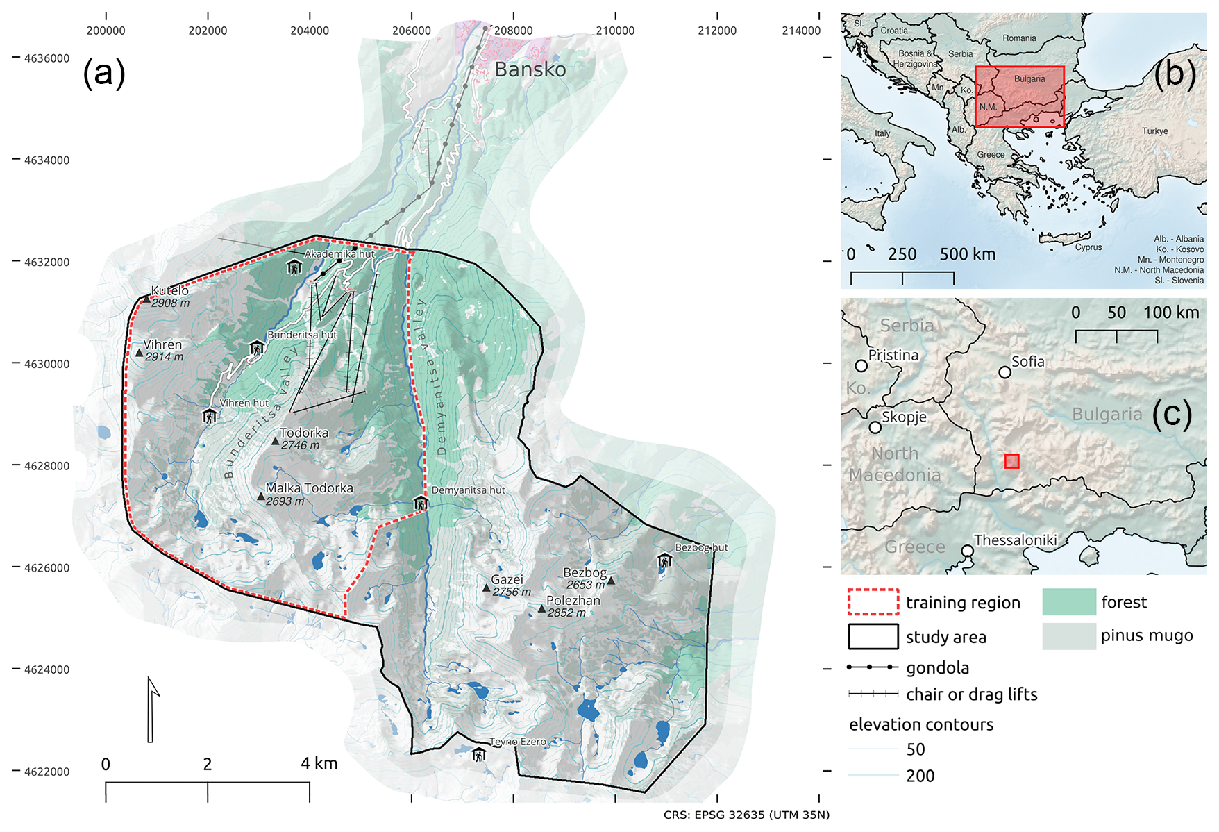
Figure 1Study area located in the Pirin Mountains, Bulgaria south of Bansko. The western part of the study area covering the Bunderitsa valley, parts of the Demyanitsa valley and parts of Bansko Ski Resort has been used for model training. The study area also comprises parts of the rest of the Demyanitsa Valley and the Bezbog area, on which the models have not been trained. The light green shading presents an approximation of the areas covered by forests. The upper boundary of these areas corresponds to the treeline level. The map utilises the following sources. (a) © OpenStreetMap contributors 2025. Distributed under the Open Data Commons Open Database license (ODbL) v1.0. FAB-DEM (https://doi.org/10.5523/bris.s5hqmjcdj8yo2ibzi9b4ew3sn). Distributed under a Non-Commercial Government Licence for public sector information. (b) and (c) Natural Earth. Free vector and raster map data at https://www.naturalearthdata.com/ (last access: 26 March 2025).
2.2 General input data
The essential input data for generating ATES maps include a digital terrain model (DTM) and at least one type of forest data, which can be chosen from several available options. In AutoATES 2.0, Toft et al. (2024) introduced three possible forest data types that can be used – percent canopy cover (PCC), stem density, and basal area.
For the majority of the study area, we used a 5 m resolution DTM provided by Pirin National Park for the purposes of this study (Pirin National Park, 2022). Additionally, for a smaller section of the Bunderitsa Valley, a 2 m DTM provided by Geopolymorphic Cloud, a private geospatial data provider, was utilised. The digital terrain models (DTMs) were derived from historical military topographic maps of Bulgaria. These maps were produced using geodetic surveys and manual cartographic techniques, with a strong reliance on field observations. Consequently, the resulting DTMs may have limited accuracy in certain locations, particularly in densely forested or rugged areas where direct observations were challenging, and smaller terrain features may have been generalised or omitted. The DTM from Geopolymorphic Cloud was generated by digitising 1:5000 topographic maps, whereas the DTM from Pirin National Park was based on smaller-scale original maps. The two datasets were merged using open-source GIS software (QGIS) and resampled to a 10 m resolution. A 10 m DTM resolution has been utilised in a number of AutoATES case studies (Larsen et al., 2020; Huber et al., 2023) and coincides with the resolution of the available forest data in our study region. Additional processing of the DTM consisted of a script-based correction of elevations inside lake polygons to ensure even lake surfaces.
Forest structure data in Bulgaria is scarce, and the dataset available from Pirin National Park lacks sufficient detail for this study's purposes. Therefore, we utilised the satellite-based open-source Copernicus tree cover density product with 10 m resolution (Copernicus, 2020). This dataset assigns a percentage value to each pixel that corresponds to varying degrees of forest density. To maintain consistency with terminology used in AutoATES 2.0 (Toft et al., 2024), we referred to this layer as percent canopy cover (PCC). While this dataset has known limitations, such as an inability to detect small forest openings and occasional misclassification of dwarf mountain pine as forest (Panayotov et al., 2024b), its open accessibility makes it a useful candidate for evaluating the potential of low-cost, large-scale mapping approaches. All datasets have been transformed to a common coordinate system (EPSG:32635, WGS 84/UTM zone 35N).
2.3 Training data
Since RF is a supervised ML algorithm (Nasteski, 2017), it requires a training dataset to learn the complex patterns and dependencies between input features and the corresponding response variable (i.e. the ATES classes). The training dataset needs to contain manually labelled ATES regions, where the assigned ATES classes are treated as the ground truth from which the RF classifier learns. Ensuring a diverse training set is critical, as it must represent a variety of possible terrain features associated with each ATES class. A well-balanced and comprehensive dataset enhances the algorithm's ability to learn the defining characteristics of the different classes (Gong et al., 2023). Additionally, the accuracy of the spatial boundaries in the training dataset is crucial. Poorly defined polygon boundaries, such as one polygon extending into a region belonging to a different ATES class, can introduce ambiguity into the model, reducing its ability to generalise to unseen data. Another key factor is class balance within the training dataset. While RF is robust to class imbalance, maintaining a relatively balanced number of samples per class generally improves model performance (Japkowicz, 2001).
In this study, the training data was delineated in cooperation with a local expert for an area covering the Bunderitsa Valley and a small portion of the Demyanitsa Valley near Bansko Ski Resort (see Fig. 1) and was based on ATES class definitions following Statham and Campbell (2025) and Toft et al. (2024). We used the simple, challenging, complex, and extreme terrain classes. Statham and Campbell (2025) also introduced class 0 – non-avalanche terrain – as an optional fifth ATES class describing terrain where avalanches do not occur. In this study we do not use this class due to specifics of our study area and concerns regarding the delineation of completely avalanche-safe zones using automated methods without prior human verification. Instead we implicitly include class 0 – non-avalanche terrain – within our definition of class 1 – simple terrain. This approach aligns with the statement of Statham and Campbell (2025) that delineation of non-avalanche terrain requires a high level of confidence and has been treated similarly in recent applications of AutoATES (Sykes et al., 2024; Toft et al., 2024).
The remainder of the Demyanitsa valley and the Bezbog region were entirely excluded during the training set development. The decision to use only a subset of the study area for training was motivated by the objective of evaluating the models' abilities to generalise beyond the region they were trained on.
The delineation of training data polygons was based on local expertise and records of well-known and observed avalanche release areas and runouts in the region. The mapping process was additionally informed by slope maps, results of dendrogeomorphologic studies (Tsvetanov and Panayotov, 2024), and local-scale avalanche simulations conducted with RAMMS (Panayotov et al., 2024a). The training set was designed to ensure diverse representation of terrain features associated with each ATES class and consists of manually delineated polygons, each assigned to one of the four ATES classes. For the majority of the training data, the borders of individual polygons do not represent the boundaries of ATES classes, but rather reflect areas that were identified as belonging to a specific class with high confidence. An exception is directly neighbouring polygons, where the border lines between adjacent polygons were also mapped with high confidence and represent class boundaries. The different shapes and sizes of the individual polygons correspond to the characteristics of associated terrain features. Areas of simple terrain are generally represented by larger, rounded features, while training polygons for challenging and complex terrain are more elongated and confined, reflecting the shapes of corresponding avalanche release and transit zones. Extreme class polygons are generally the smallest and most precisely defined, as they correspond to single rock faces, cliff bands, and generally very steep terrain. They were also refined using a slope map. Using smaller, clearly defined polygons for training facilitated labelling of regions with high confidence, ensuring accurate classification. In contrast, we found that manually drawing a continuous ATES map for the entire study area is significantly more challenging and may introduce generalisation errors, making it more difficult for the classifier to learn effectively.
Efforts were also made to achieve class balance as much as possible across the simple, challenging, and complex categories. However, the extreme class was underrepresented due to the more limited availability of extreme terrain in the study area. While the training dataset was carefully constructed, we acknowledge that relying solely on the assessment of a single avalanche expert, rather than a larger group due to limited resources, may introduce some degree of bias. Figure 2 illustrates the training data polygons used in this study, as well as the used PCC data for the same region.
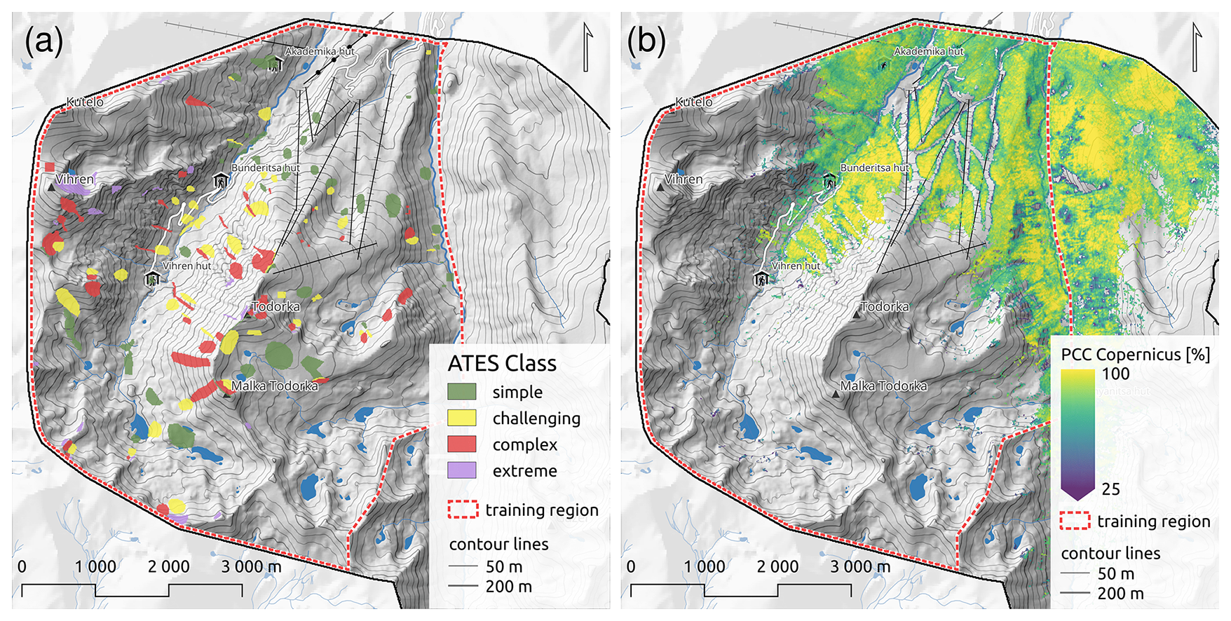
Figure 2(a) Training data based on local expert assessment of ATES classes for the training area, covering the Bunderitsa Valley and parts of the Demyanitsa Valley. (b) Copernicus percent canopy cover (PCC) layer for the training region.
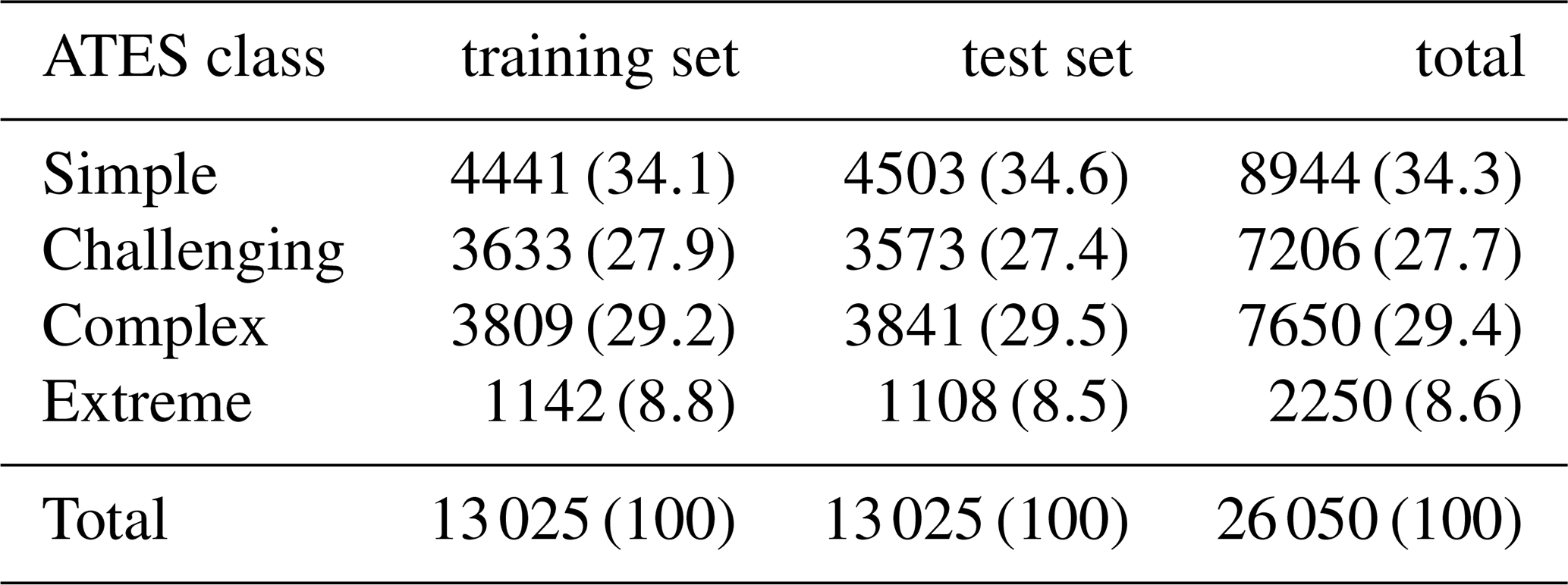
The training polygons were subsequently converted to a 10 m raster dataset and aligned with the other raster input features described in Sects. 2.2 and 2.4. The dataset was then randomly split into a train–test partition, with one half used for model training and the other reserved as a hold-out test set to evaluate performance and generalisation (see Sect. 2.5). Table 1 presents the total number of pixels for each ATES class and the approximate split between training and test sets. Figure A3 displays the distributions of some of the most important input features across each of the four ATES classes in the training dataset.
Table 1Distribution of ATES classes in the training set and test set. Numbers correspond to the number of 10 m×10 m pixels, multiplication with 102 yields area in m2. The relative share of each class in % is provided in brackets.
2.4 AutoATES model chain
The basic AutoATES model chain (e.g. Larsen et al., 2020; Huber et al., 2023; Panayotov et al., 2024b; Sykes et al., 2024; Toft et al., 2024) is based on open-source components developed by different research groups. It has been designed to work with limited input data requirements (DTM, forest layer), and involves three main steps. These steps comprise (1) the identification of potential avalanche release areas (PRAs), (2) the delineation of potential avalanche runouts originating from the PRAs, and (3) a final classification and mapping step, which has been referred to as the “AutoATES classifier” in previous studies (Sykes et al., 2024; Toft et al., 2024). This study focused on the application of supervised ML methods, specifically RF models, in the final AutoATES classification step in place of the previously proposed deterministic, expert-based set of thresholds and rules (Fig. 3). The next sections provide an overview of the setup and parameterisation that have been used in the PRA and avalanche runout modelling steps in this study, and briefly discuss the ”classic” decision tree-based AutoATES classifier, before Sect. 2.5 introduces the modifications to the classifier investigated in this study.
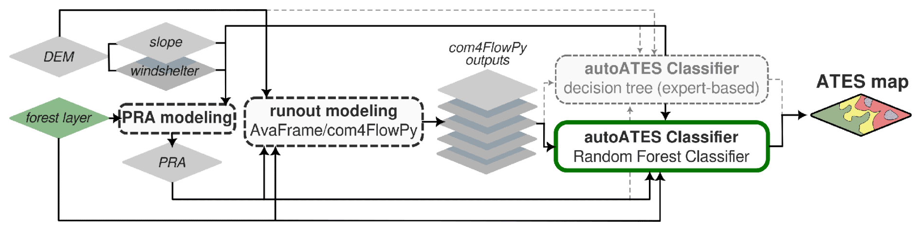
Figure 3Main components of the AutoATES model chain (represented by rounded rectangles) and model's input, intermediate, and output layers (depicted as diamond shapes). Parts of the model chain that are shared with the approach of Toft et al. (2024) are highlighted with dashed outlines. The introduction of RF techniques in the AutoATES classifier, as investigated in this study, is indicated by a green outline.
2.4.1 Modelling of potential avalanche release areas (PRAs)
The PRA model used in this study followed the approach outlined by Toft et al. (2024) and Sykes et al. (2024). The original PRA model proposed by Veitinger et al. (2016a) has been modified by Sharp (2018), Schumacher et al. (2022) and Toft et al. (2024) to include forest information and operate on input data with coarser resolution (≈10 m as opposed to 2 m used by Veitinger et al., 2016a). The model maps a set of input layers (slope, wind shelter, PCC) to fuzzy membership values μ using three-parameter bell-shaped membership functions with varying parametrisations (Eq. 1).
The fuzzy membership values of the three layers are then combined with a ”fuzzy AND” operator (Werners, 1988) to a continuous PRA membership value , which indicates PRA likelihood (Eq. 2).
We used a DTM and the Copernicus PCC layer, both at 10 m resolution, as inputs for the PRA model. To parametrise the bell-shaped membership functions, we adopted values for slope, wind shelter, and PCC from Toft et al. (2024), with a slight modification to the Cauchy membership function for slope. To maintain comparability with previous applications of AutoATES in the study area (Panayotov et al., 2024b), we assigned membership values of 0 to areas with slopes <28° or >60°. This approach aligns with previously proposed methods for PRA delineation (Veitinger et al., 2016b; Bühler et al., 2013, 2018), but differs slightly from the procedure reported by Toft et al. (2024), which assigns low, but non-zero membership values in these areas.
To convert the continuous PRA membership values into a binary PRA layer , we applied a threshold value of 0.3. This binarisation is required for the subsequent runout modelling step. The threshold was selected based on experience from previous studies (Hesselbach, 2023; Huber et al., 2023; Panayotov et al., 2024b), site inspections, and local expert knowledge. Figure A1a and b present the results of the PRA modelling step (PRAcont, PRAbin) for the terrain surrounding Todorka Peak, which is easily accessible from the top chairlift of Bansko Ski Resort.
2.4.2 Modelling of avalanche runout and intensities with com4FlowPy
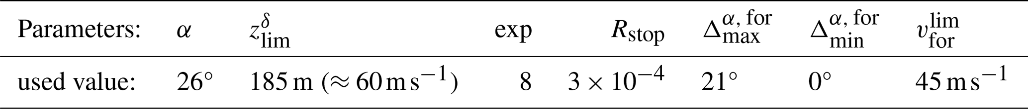
AutoATES utilises the empirical, raster-based model Flow-Py (D'Amboise et al., 2022) for calculations of avalanche runouts and intensities from the binary PRAs identified in the previous step (Sykes et al., 2024; Toft et al., 2024). Flow-Py has been integrated into the Open Avalanche Framework AvaFrame (Oesterle et al., 2025) in 2024 and is now available as AvaFrame module com4FlowPy (Huber et al., 2024). In this study we utilised com4FlowPy with its forest-friction option enabled (D'Amboise et al., 2021; Huber et al., 2024). The forest-friction functionality is used to account for increased energy dissipation in forested areas by increasing the basal friction on forested cells in the model domain. The basal friction increase on forested cells is modulated by a lumped forest structure index (FSI) and modelled avalanche intensities zδ (D'Amboise et al., 2021; Huber et al., 2024). The FSI layer used in this study was obtained by linearly scaling the Copernicus PCC layer (Fig. 2b) to the interval , where 0 represents no forest and 1 represents dense forest canopy cover. The model parameters used for com4FlowPy are listed in Table 2. Initial values of α, , exp and Rstop were based on previous studies (Hesselbach, 2023; Huber et al., 2023; Panayotov et al., 2024b). Further parameter refinement to local conditions was informed by empirical relationships proposed by Bakkehøi et al. (1983) and McClung and Gauer (2018), as well as comparative simulations with a physically-based model (Tonnel et al., 2023) for selected avalanche tracks. The parametrisation of the forest-friction function was informed by a limited sensitivity study (Huber et al., 2024). Although a rigorous evaluation of the modelled avalanche runouts was beyond the scope of this study, good agreement was found between the model results, local records of historical avalanches, and dendrochronological investigations in the Bunderitsa area (Panayotov and Tsvetanov, 2024; Tsvetanov and Panayotov, 2024) using the proposed parameters.
Table 2Parameters used for modelling of avalanche runouts and intensities with com4FlowPy.
Com4FlowPy computes several model outputs in the form of raster layers (D'Amboise et al., 2022), which can be used to characterise avalanche intensities, proximity to release areas, and overhead exposure (Sykes et al., 2024). Recent studies have used different combinations of output layers from com4FlowPy in applications of AutoATES (Schumacher et al., 2022; Sykes et al., 2024; Toft et al., 2024). In this study, we focused on the maximum modelled energy line height , the maximum modelled local travel angle (γ), cell counts, and the sum of modelled fluxes (∑routFlux) (see Fig. A1c–f). The output layer can be interpreted in terms of potential avalanche intensities and more intuitively be converted to maximum potential avalanche velocities by (Körner, 1980). The maximum local travel angle (γ) provides a measure of the proximity of a potential runout location to the nearest PRA, taking into account both the distance and the average gradient of the avalanche path connecting the two locations (D'Amboise et al., 2022). The cell counts layer describes the number of PRA cells potentially affecting a location, while the ∑routFlux layer sums the modelled flux that is routed through a cell (D'Amboise et al., 2022). Both layers provide an estimate of potential overhead hazard, with high values typically characterising gullies and/or overlapping avalanche paths (Fig. A1e and f). While the cell counts output focuses on the sizes of overhead PRAs, ∑routFlux provides a more nuanced output, highlighting terrain traps such as gullies and deposit zones.
2.4.3 AutoATES classifier
The final step in the AutoATES model chain – the AutoATES classifier – combines layers derived from preceding stages of the model chain (PRAs, runout and intensity outputs, slope, and forest information) into ordinal ATES ratings. Although the specific configuration of input layers employed by the AutoATES classifier varies slightly across different versions of AutoATES (Larsen et al., 2020; Schumacher et al., 2022; Toft et al., 2024) and its local applications (von Avis et al., 2023; Huber et al., 2023; Panayotov et al., 2024b), the underlying classification methodology has remained largely consistent since the release of AutoATES v1.0 (Larsen et al., 2020).
In summary, existing AutoATES classifiers are based on a deterministic framework that applies expert-defined thresholds and rules to derive ATES ratings from a set of input layers. This rule-based approach offers the advantage of being transparent and interpretable from a human perspective, and also mirrors the general structure of both the original and updated ATES technical models suggested for manual ATES mapping (Statham et al., 2006; Statham and Campbell, 2025).
However, to eliminate the need for parameter optimisation (Sykes et al., 2024) or rule modification (Panayotov et al., 2024b) when applying AutoATES to new regions, this study tested an alternative classification approach based on RF models.
2.5 Random Forests
2.5.1 Basic principles
RF is a supervised ML algorithm based on ensemble learning, designed for both classification and regression tasks (Breiman, 2001). In the context of ATES class prediction, the model operates on a per-pixel basis, assigning each pixel one of four possible terrain classes: simple, challenging, complex, or extreme. The algorithm constructs multiple decision trees during training, linking input features that describe the characteristics of each pixel to its manually labelled ATES class. Each individual tree generates a class prediction, and for a new, unseen data point, the RF aggregates predictions from all trees, assigning the most frequent class as the final output. This ensemble approach reduces overfitting compared to a single decision tree, enhancing model robustness and generalisation performance (Breiman, 2001).
Each tree in the RF is trained using either a bootstrap sample (random sampling from the training dataset with replacement) or the entire dataset, as controlled by the bootstrap parameter. During tree construction, the algorithm determines the optimal split at each node by selecting a feature and a threshold that minimises impurity, commonly measured using Gini impurity and information gain (Prasetiyowati et al., 2021). Impurity measures quantify the degree of class heterogeneity within a dataset. A node containing only samples from a single ATES class has zero impurity, whereas a node with an evenly distributed mix of classes exhibits higher impurity. The goal of decision tree construction within the RF is to iteratively partition the data so that the resulting subsets (leaf nodes) are as pure as possible. This process is guided by information gain, which quantifies the reduction in impurity achieved by a particular split. At each decision node, the algorithm evaluates a subset of input features (determined by the max_features parameter) and identifies the feature and threshold that maximise information gain. The search space for threshold values is usually restricted to midpoints between unique observed values within the selected feature, ensuring computational feasibility while optimising for split quality (Salman et al., 2024).
The RF algorithm has several hyperparameters that control the training process. While in-depth optimisation of hyperparameters is beyond of the scope of this study, a basic evaluation on how tuning a few key parameters affects model performance was conducted (see Sect. 2.5.2).
2.5.2 Application of RF for ATES mapping
Following the procedure outlined in Sect. 2.4, a series of raster layers were generated in the PRA and avalanche modelling steps. Together with the general input data layers (Sect. 2.2), these layers served as input features for three different RF models investigated in this study – RF1, RF2, and RF3.
For all models, both the training labels and the input features were stored in georeferenced TIFF files with identical dimensions and pixel resolutions. Each input feature was represented as a separate raster band within the input feature files. The implementation was realised in Python 3.9.21 (Python Software Foundation, 2024), leveraging libraries such as GDAL and NumPy for data processing, while scikit-learn (Pedregosa et al., 2011) was used to define and train the RF classifiers.
The scikit-learn library provides extensive control over the model's hyperparameters, enabling their optimisation to enhance generalisation and predictive performance. Hyperparameter tuning is a widely researched topic, with numerous studies dedicated to optimising model configurations (Ramadhan et al., 2017; Probst et al., 2019; Siji George and Sumathi, 2020; Contreras et al., 2021; Wang et al., 2021; Bischl et al., 2023; Rimal et al., 2024). However, previous research has also demonstrated that the default hyperparameter settings of the RF algorithm generally yield strong predictive performance (Probst et al., 2019). In this study, we adopted the approach of Contreras et al. (2021), using their predefined parameter grid with minor modifications. We also added the bootstrap parameter to the hyperparameter search together with max_samples. If bootstrap is set to false, the entire training dataset is used to build each tree. If it is set to true, then max_samples (as a fraction from all samples) training points are selected at random, with replacement, from the full training set. Finally, we also introduced the class_weight parameter, which can help training when classes are imbalanced, as was the case with the extreme class in our training set. The parameters max_depth, max_leaf_nodes, min_samples_leaf, and min_samples_split together control how much the trees grow, preventing overfitting to the training dataset and ensuring the model generalises better to new data.
The complete hyperparameter grid, along with a brief description of each parameter, is presented in Table 3. All unspecified parameters remain at their default values. Given computational constraints, we opted for a random search strategy rather than an exhaustive grid search, which would otherwise result in an infeasible number of combinations. Specifically, we sampled 10 000 hyperparameter combinations at random from the defined grid.
Table 3Hyperparameter setup for training the RF models (RF1–3).
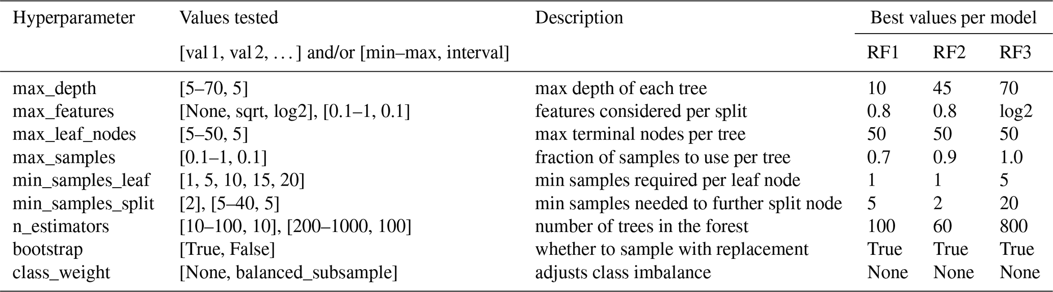
Decimal values or functions should be interpreted as that fraction of the total number. For example, for the max_features hyperparameter, sqrt means try the square root of the total number of features as the value, while 0.1 means try 10 % of the total number of features. None means that there is no limit or a parameter is not used.
To evaluate model performance, the training dataset was randomly partitioned into training (50 %) and test (50 %) sets, ensuring that the test set remained entirely separate from the training process. Although a train-test split is less common than ratios such as or , it has nevertheless been reported in previous studies (Joseph, 2022; Afendras and Markatou, 2019). Given the sufficiently large sample size in our case, we decided to allocate a relatively larger portion of labelled pixels to the test set to obtain robust estimates of model performance and generalisation capability while reducing computational requirements for model training.
Additionally, we employed k-fold cross-validation with k=3 (Varoquaux and Colliot, 2023), wherein the training set was further subdivided into three equal partitions (folds). Each fold alternates between training and validation, with two folds used for training while the third serves as the validation set. This process is repeated across all fold combinations, allowing the model to select the hyperparameter configuration that maximises accuracy on the validation folds. The best combination of hyperparameter values found per model is also displayed in Table 3.
Feature selection plays a crucial role in model development, as the accuracy of an RF classifier relies heavily on the relevance of input features (Rogers and Gunn, 2006). Initially, we adopted a feature set as proposed by Huber et al. (2023) that was also utilised in a previous AutoATES application in Bulgaria (Panayotov et al., 2024b). The feature set consisted of slope, PCC, a binary-thresholded PRA (PRAbin) layer, and the maximum modelled local travel angle (γ). The goal at this stage was to address the first research question – whether an RF model can effectively replace manually designed classification trees. This first model trained on these four features is referred to as RF Model 1 (RF1).
Next, we investigated whether RF can provide additional insights into feature importance and whether incorporating more input features enhances performance. Since the algorithm records the features used at each decision node, feature importance can be calculated to reveal which features most influence ATES classification. The first modification involved replacing the binary PRA layer with its continuous counterpart (PRAcont) to leverage the full range of information it provides, rather than reducing it to categories prematurely. We then investigated whether additional com4FlowPy outputs could enhance classification. A limitation of RF1, which mirrors AutoATES Austria's inputs, is its lack of consideration of overhead exposure or avalanche intensity (Huber et al., 2023), which were utilised in other studies by incorporating additional com4FlowPy output layers in the final AutoATES classification step (Sykes et al., 2024; Toft et al., 2024).
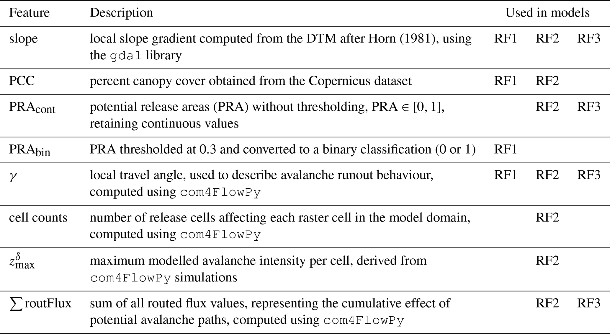
In our approach, after replacing PRAbin with its continuous counterpart, we incrementally introduced cell counts, , and the sum of modelled routing fluxes (∑routFlux), training a new model for each using the same parameter grid as shown in Table 3. This incremental addition of features aimed to assess the impact of each individual feature on the overall classification performance. After incorporating all additional features, we constructed a seven-feature model, referred to as RF Model 2 (RF2). We refrained from including additional features beyond these to maintain comparability with existing AutoATES approaches and minimise multicollinearity among input features, which can reduce the interpretability of model results. Based on the feature importance rankings of model RF2, we identified the four most influential features – ∑routFlux, slope, local travel angle (γ), and PRAcont – and used them to train a final model, RF Model 3 (RF3). A summary of the features used and their descriptions is presented in Table 4.
Horn (1981)Table 4Description of input features and the corresponding models (RF1–3) in which each feature was used. More detailed information on each feature is provided in Sects. 2.2 and 2.4.
After training the three models, we applied them to classify the pixels in the test set and evaluated their performance using a range of metrics, as detailed in Sect. 2.6. We also applied the models to the entire study area, including the Bunderitsa, Demyanitsa, and Bezbog valleys, to qualitatively assess their generalisation and performance across different regions.
The RF algorithm also produces an additional output that reflects the confidence of its predictions. For each data point, the model generates four probability values, each indicating the likelihood of belonging to a specific ATES class. The class with the highest probability is selected as the final prediction. Higher confidence is achieved when a larger proportion of decision trees in the forest agree on the same class (Bhattacharyya, 2011). We generated rasters that visualise the model's confidence in the predicted ATES classes across the entire study area. Additionally, we analysed the distribution of predictive confidence for each model and examined how it varies across different ATES classes.
It is essential to emphasise that all random processes involved in model training, such as the train-test split, model initialisation, and random selection from the hyperparameter grid, were consistently performed using a fixed seed. Using the same seed ensures that, despite the randomness of these steps, they produce identical results each time they are executed (Dutta et al., 2022). As a result, the train-test split remained unchanged across all three models (RF1, RF2, RF3), and the same set of hyperparameter combinations was explored. Keeping these factors constant enabled a more reliable comparison between models, ensuring that any observed differences were attributable to variations in the input features rather than differences in training data or hyperparameter selection.
2.5.3 Complementary analyses
While we strived for a balance of ATES classes in constructing the training dataset, we found that the ratio of forested (PCC>0) to non-forested (PCC=0) pixels was unevenly distributed (6 415:19 635 (24.6 %–75.4 %)). This ratio reflects both the distribution of forested and non-forested areas in the training region (see Fig. 2) and the general tendency for more severe avalanche terrain to occur outside forested areas. To assess the potential impact of this imbalance, particularly on reported feature importances, we constructed a balanced training subset containing an equal number of forested and non-forested pixels. While all original 6415 forested training pixels were retained, the same number of non-forested pixels was randomly sampled from the original 19 635 non-forested pixels. We then trained an additional RF model (referred to as model RF1 balanced), with features identical to RF1, on this modified training dataset to investigate how the reported feature importances for the balanced training dataset compared to those obtained using the full dataset (see Sect. 2.3).
2.6 Methods used for performance evaluation
To assess model performance, we computed several evaluation metrics on the test set, including accuracy and the per-class precision, recall, and F1 score (Rainio et al., 2024). Estimation based on a held-out test set has been shown to offer reliable estimates of model generalisation performance in previous studies (Varoquaux and Colliot, 2023).
The most fundamental metric is accuracy. It is defined as the proportion of correctly classified predictions out of all pixels in the test set (Eq. 3):
While accuracy is useful, it does not provide insight into how well the model performs for each individual class, especially in imbalanced datasets, as was the case with the extreme terrain class. Therefore, we also computed precision, recall, and F1-score, using binary confusion matrices for each class containing the numbers of True Positive (TP), True Negative (TN), False Positive (FP), and False Negative (FN) predictions.
Precision is defined as the proportion of instances predicted to belong to a class that are actually members of that class – in other words predicted correctly. It is calculated as:
Recall is defined as the proportion of instances that actually belong to a certain class and are correctly predicted as belonging to that class. It is calculated by:
The F1 score is the harmonic mean of precision and recall, providing a balanced measure of model performance. It is calculated by:
In addition to the per-class skill-scores, we also computed the weighted mean of each metric by weighting the per-class metrics according to the proportion of each class in the test set. The raw numbers used for calculating the evaluation metrics were also visualised in a multi-class confusion matrix. The full confusion matrix allows for a more detailed interpretation of model predictions compared to the test set. For example, distinctions between instances where model predictions differ from the true labels of the test data by only one ordinal class and more severe instances of misclassification can be made (Rainio et al., 2024).
Another common method to evaluate model performance for classification tasks are plots of the precision-recall curve and evaluation of the associated areas under the curve (AUC). The precision-recall curve visually represents the trade-off between precision and recall as the decision threshold is varied. The decision threshold defines the probability above which an instance is classified as belonging to a particular class. For example, if the threshold is set to 0.5 and the maximum predicted probability for a class is 0.4, the instance will not be assigned that class, as its probability does not exceed the threshold. Precision and recall are both influenced by the threshold. As the threshold decreases, recall tends to increase while precision may decrease, and vice versa. The curve is useful for evaluating model performance, especially in the case of imbalanced classes, with a larger area under the curve indicating better overall accuracy (Rainio et al., 2024). In this study, we produced class-wise precision-recall curves for all three trained models and calculated the corresponding AUCs. The precision-recall curve was chosen over the commonly used receiver-operator curve (ROC), which plots the true positive against the false positive rate, due to its more robust performance in the presence of class imbalances.
In addition to the quantitative methods used to evaluate the models' performances on the test set, we conducted a qualitative assessment of model predictions across the entire study area and compared them with the results of a previous local adaptation of AutoATES in the study area (Panayotov et al., 2024b). These qualitative comparisons also emphasised regions outside the training area, thereby providing initial insights into the models' generalisation capabilities.
3.1 Quantitative evaluation against test set
Table 5 presents the full multi-class confusion matrices for each model, comparing the model predictions against the held-out test set. The area overlap between the predicted and the actual ATES classes for each class and each model is provided. Since each pixel represents an area of 100 m2, the number of overlapping pixels can be calculated by dividing the area value by 100. The diagonal of the matrix, highlighted by bold numbers, represents correct classifications, while misclassifications below the diagonal correspond to underclassification errors (lower ATES class predicted than actual one), and those above it indicate overclassification errors (higher ATES class predicted than actual one). Model RF1 has 1669 overclassified pixels out of the total 13 025 in the test set (12.81 %) and 1026 underclassified pixels (7.9 %). Model RF2 has 1242 overclassified pixels (9.54 %) and 1061 underclassified pixels (8.15 %). Model RF3 has 1497 overclassified pixels (11.49 %) and 1053 underclassified pixels (8.08 %). For each model, none of the simple class pixels in the test set were misclassified as extreme, and only three extreme class pixels were incorrectly predicted as simple, representing a very small proportion of the total misclassifications. Additionally, the confusion matrices show that nearly all classification errors involve a misclassification by only a single class level. The confusion matrix presents the raw class counts, which were used as the basis for deriving the subsequent evaluation metrics.
Table 5Multi-class confusion matrices for models RF1, RF2, and RF3. Absolute values for area overlap are provided in m2, division by 100 yields number of pixels/predictions. Values in bold along the diagonals correspond to correct predictions; values below and above the diagnoals show under and overclassifications respectively.
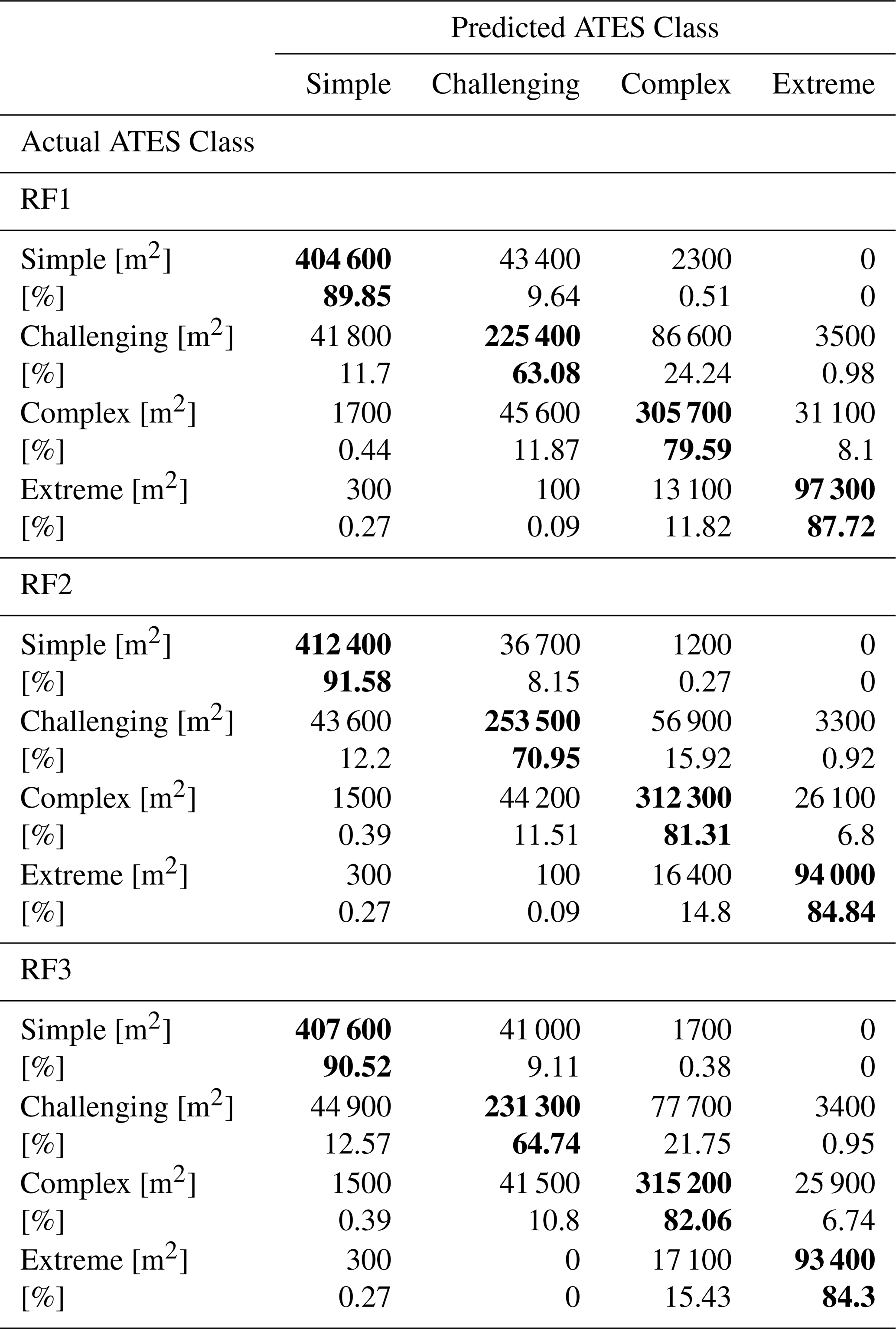
The overall accuracies for each model are 79.31 % for RF1, 82.32 % for RF2, and 80.42 % for RF3. These results indicate that model RF2 achieves the highest overall accuracy, followed closely by model RF3, which performs slightly better than model RF1 in terms of correct predictions.
Figure 4 displays the additional class-wise evaluation metrics for all models, calculated against the test set. Notably, for all three models, the precision, recall, and F1-scores for the simple terrain class are higher than for the other ATES classes, averaging around 90 %. The calculated metrics for the challenging class are consistently the lowest across all three models, while the metrics for the complex and extreme classes generally fall between those of the simple and challenging classes. Furthermore, for model RF1, the extreme class exhibits a high recall of 87.8 % on the test set, with similar recall values of around 85 % observed for the other models.
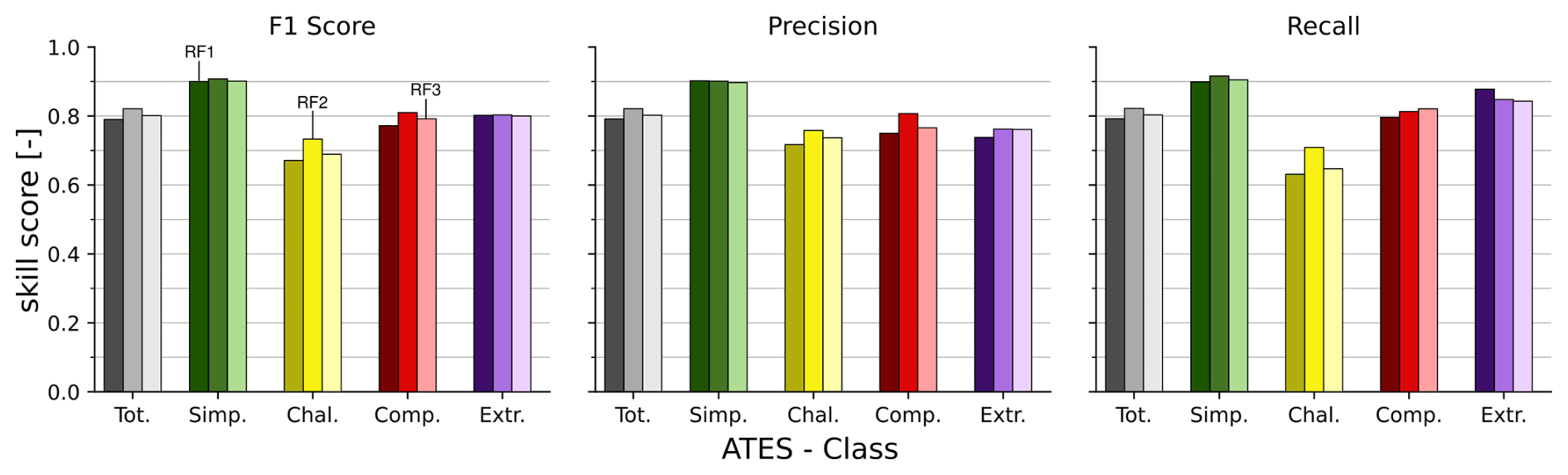
Figure 4Per-class skill-scores for the three RF models: RF1 (left), RF2 (middle), and RF3 (right), based on the test set. Total scores for the F1 score, precision and recall metrics are calculated as the weighted mean of class-specific scores. Tot.: total, Simp.: simple, Chal.: challenging, Comp.: complex, Extr.: extreme.
These general trends are also reflected in the precision-recall curves displayed in Fig. 5. In terms of this evaluation method, all three models exhibit the highest predictive capacities for the simple ATES class, while the challenging class consistently scores the lowest in computed AUC values. Predictive capacities for the remaining two ATES classes fall between the simple and challenging classes, with overall AUC values being highest for model RF2, followed by RF3 and RF1. Similar to the other utilised evaluation metrics, the variance between ATES classes is generally more pronounced than the differences between the three trained models.
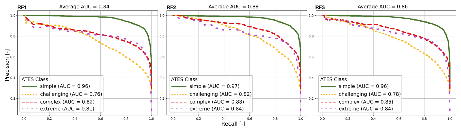
Figure 5Precision-recall curves for each RF model (RF1–3), shown per class, and the corresponding areas under the curve (AUC).
3.2 Predictive confidence
Figure A2 shows maps of the predicted ATES classes for all three RF models (panels a–c) along with the prediction probabilities (panels d–f) for the entire study area. General patterns for both the ATES class predictions and the associated prediction probabilities appear to follow similar trends across all three RF models, with higher predictive confidence generally associated with the simple ATES class.
A closer look is provided in Fig. 6, which zooms in on an area of the study region surrounding Todorka Peak and the top chairlifts of Bansko Ski Resort. Figure 6a shows the raw 4-class predictions of the RF2 model, while Fig. 6b additionally depicts the model's prediction probabilities for each ATES class, represented by intra-class colour shading. Darker colours indicate higher prediction confidence. In this example, generally high prediction confidence is associated with areas identified as simple terrain, but other trends can also be observed. Notably, there is a general pattern of higher predictive confidence at the center of individual terrain features associated with a specific ATES class, while predictive confidence tends to decrease near the boundaries between classes.
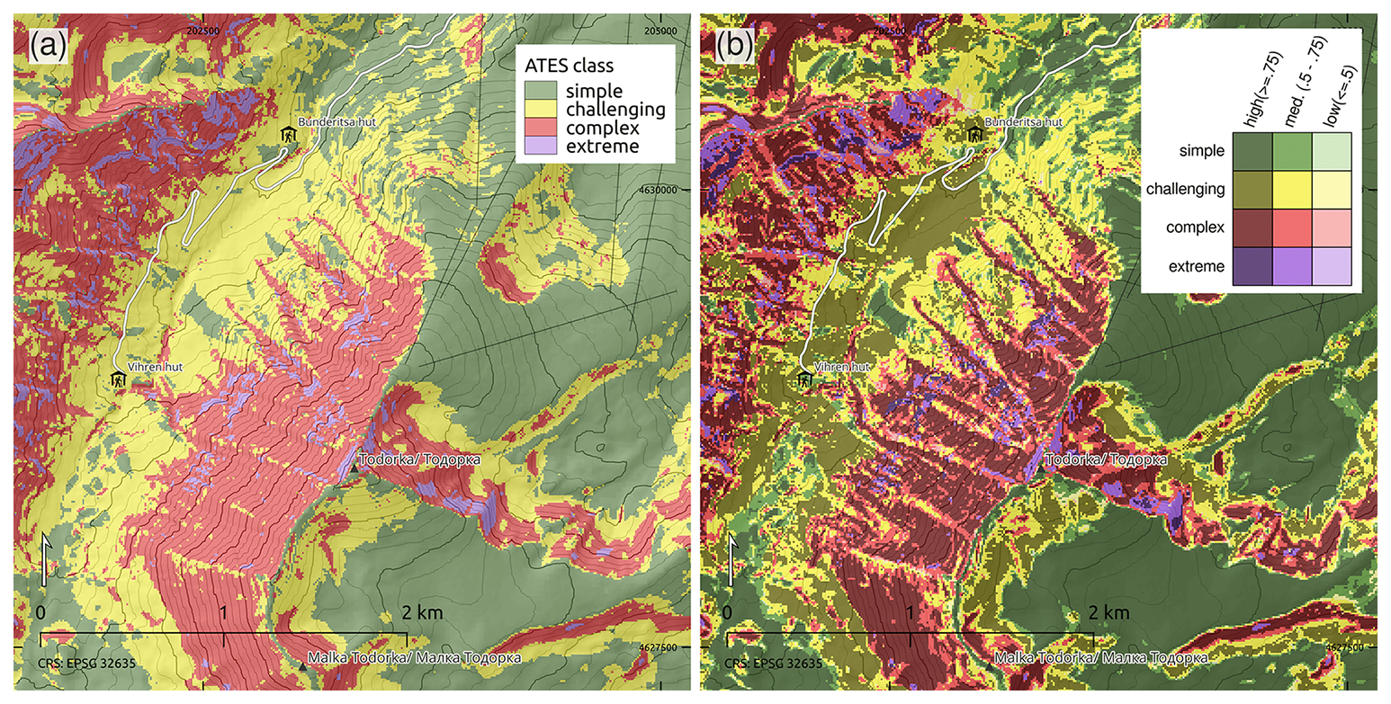
Figure 6(a) Detail of ATES class predictions using model RF2 for the area around Todorka Peak and Bunderitsa Valley. The steep west and north-east faces of Todorka are accurately classified as the complex and extreme ATES classes. (b) Example for additional visualisation of model prediction probabilities for RF2 in the same area. Model confidence is represented using colour shadings, with darker shades indicating higher prediction probabilities: high confidence ≥0.75, medium confidence 0.5–0.75, low confidence ≤0.5.
An alternative visualisation of the distributions of prediction probabilities for each ATES class across all three models is provided in Fig. 7. While this perspective confirms the general trends observed in the previously mentioned maps, it also reveals more nuanced variations in prediction probabilities between the three models. All three models clearly show the highest predictive confidence for simple terrain, with generally lower confidence for challenging terrain. Also, the confidence for the challenging class is slightly lower on average for models RF2 and RF3 as compared to model RF1. However, models RF2 and RF3, in particular, exhibit relatively high confidence in predicting large proportions of complex terrain. Notably, the bimodal distributions of prediction probabilities for complex terrain in model RF1 and extreme terrain in model RF2 are characteristics that do not become apparent from the general evaluation metrics (Sect. 3.1) or the visual inspection of maps (Figs. 6 and A2).
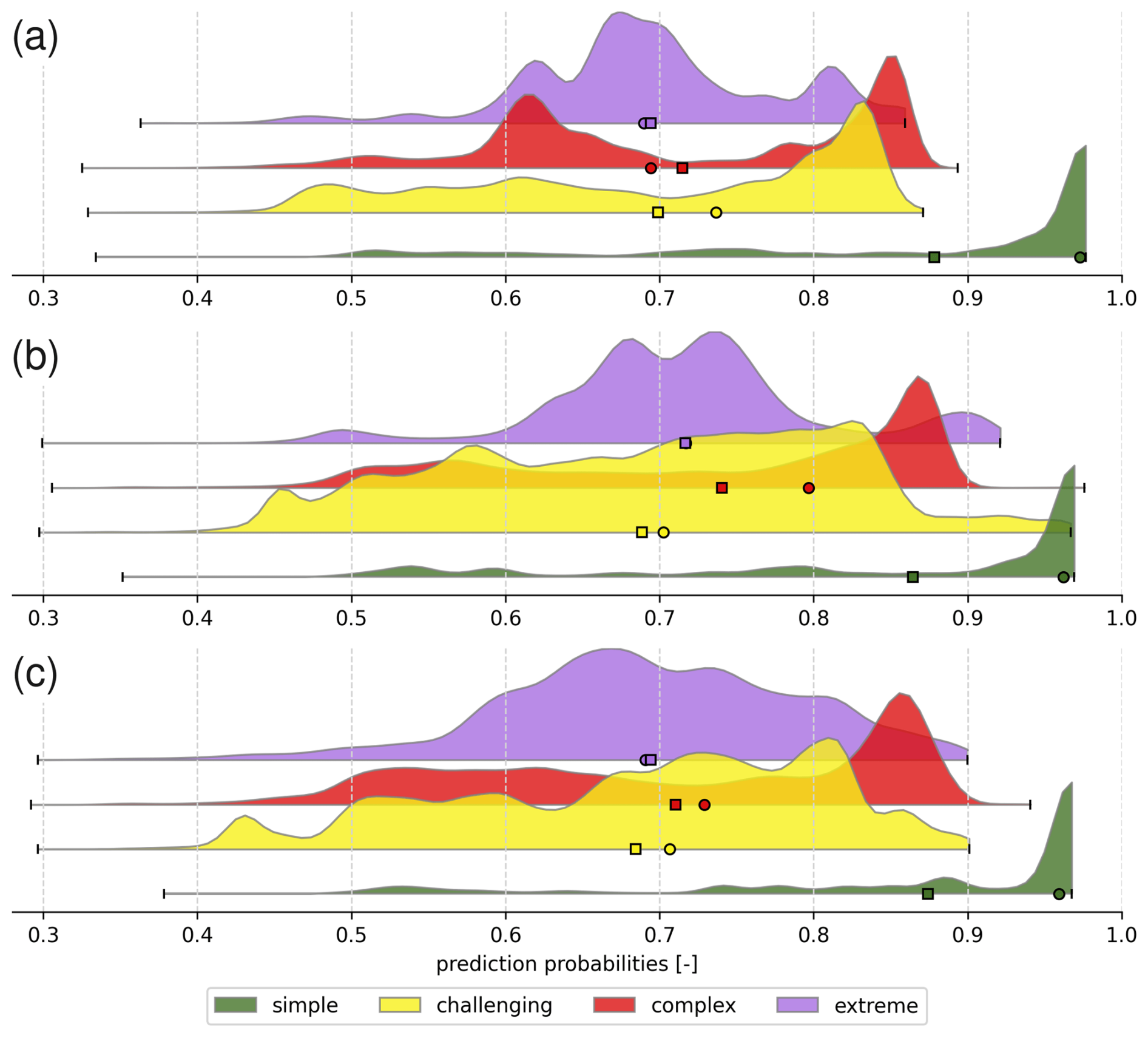
Figure 7Distributions of prediction probabilities for each ATES class and RF model across the entire study area. (a) RF 1 (b) RF2 (c) RF3. The means and medians of each distributions are indicated by the square and circle symbols respectively. The distributions for each ATES class in the panels are ordered from top to bottom as extreme, complex, challenging, and simple.
3.3 Feature importance analysis
As outlined in the introduction, a defining feature of RFs is their ability to provide information on the relative importances of input features, alongside the model predictions and associated probabilities described in the previous sections. Figure 8 visualises the relative feature importances for each of the three trained models. Terrain inclination (slope) has been used as an input feature in all three RF models and consistently ranks among the top two in terms of feature importance. Similarly, the second input feature used in all models, local travel angle (γ), also ranks within the top three most important input features for all models, indicating that this information plays a significant role in model decision-making. The ∑routFlux output from com4FlowPy has only been included in models RF2 and RF3, but is considered the most important input feature for both models, albeit with a slight margin. At the opposite end of the spectrum, the PCC information consistently ranks last for feature importance among the models it has been used in. Also, the modelled avalanche intensities appear to have relatively minor importance for RF2.
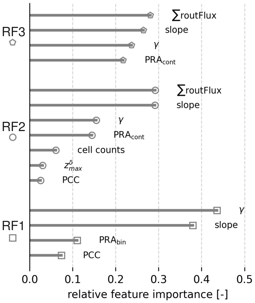
Figure 8Relative feature importances for models RF1, RF2, and RF3, highlighting the contribution of each input feature to the model's decision-making process.
The results of the complementary study conducted on the modified training dataset containing an equal share of forested and non-forested pixels (see Sect. 2.5.3) are presented in Table A2 alongside the feature importances reported for model RF1, which was trained on the full training dataset. Notably, for the balanced training dataset (model RF1 balanced), the reported feature importance for PCC remains comparatively low (0.089) and does not differ significantly from that for RF1 (0.074). Feature importances for the three other features are also very similar, and the relative ordering of features remains identical.
3.4 Comparison with field assessments and a deterministic AutoATES approach
In order to assess the general ability of the trained RF models to generalise to previously unseen terrain, we qualitatively compared model predictions for areas outside the training region with local terrain assessments at selected locations.
Figure 9 shows two examples comparing the ATES class predictions from the best-performing model, RF2, with photographs of actual winter terrain around Bezbog and Gazei Peaks. Annotated arrows highlight the corresponding terrain features between photographs and the ATES predictions overlaid on satellite imagery. In both examples, model predictions align well with on-site assessments of the avalanche terrain characteristics. The prominent terrain features visible in the photographs are also accurately recognised by the model. For instance, in the Bezbog Peak region, the broad, relatively flat ridge (indicated by arrow 2), which represents the standard winter ascent route, is correctly identified as simple terrain. Similarly, in the Gazei Peak area, prominent cliff bands (arrows 2 and 4) are correctly classified as extreme terrain in the ATES map. This visual comparison highlights the model's effectiveness in classifying avalanche terrain characteristics in previously unseen regions.
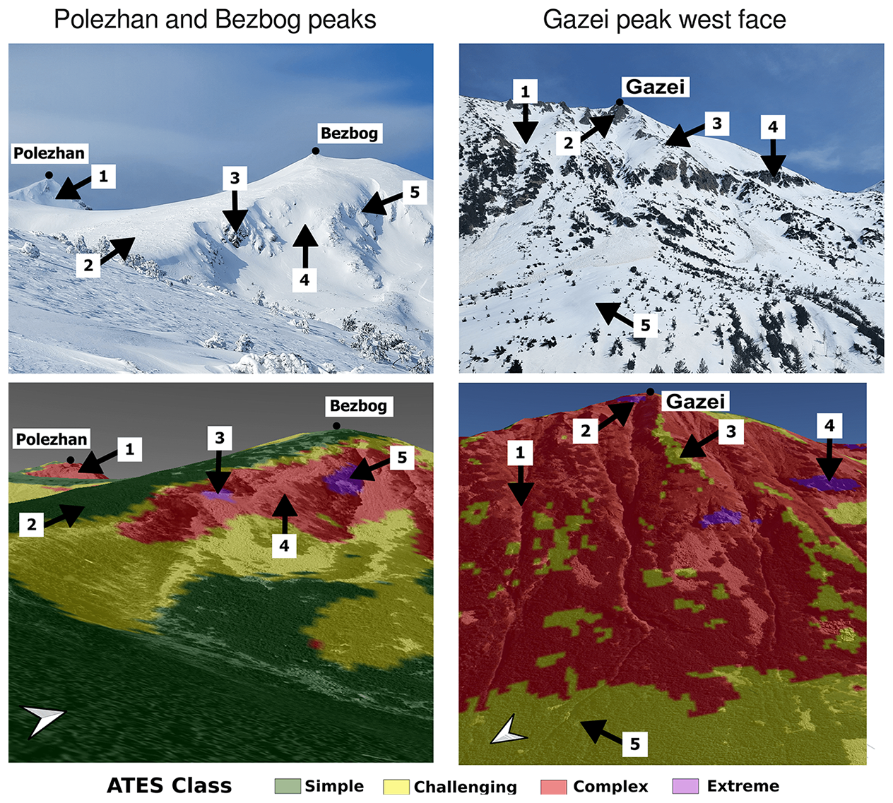
Figure 9Exemplary extract of the ATES map from model RF2 for two separate areas outside the training region – Gazei Peak and Bezbog Peak – along with photographs of the winter terrain. The base imagery over which the ATES maps are overlaid is sourced from ©Google Earth. The annotated arrows highlight the corresponding terrain features between the photographs and the ATES predictions.
Results of the comparison between a deterministic AutoATES model previously applied in the study region (Panayotov et al., 2024b) and our best performing model, RF2, are presented in Fig. A4 and Table A1. Visual side-by-side comparison for regions below (Fig. A4 left) and above the treeline (Fig. A4 right) shows that above-treeline results are very similar for both models, whereas more pronounced differences appear in sparsely forested areas below the treeline. More specifically, the deterministic model tends to predict lower ATES classes (simple and challenging) in steep, sparsely forested areas highlighted in the figure, while RF2 predicts complex and challenging terrain more consistent with on-site conditions, a pattern also observed in other locations. Despite these local differences, the predicted distribution of ATES classes across the entire study region follows a similar pattern for both models (see Table A1). While overall predictions of RF2 appear slightly more conservative, consistent with the qualitative visual comparison, the proportions of terrain assigned to each ATES class differ by a maximum of 2 %–3 %.
4.1 Potential of RF classifiers in AutoATES model chains
Our results demonstrate that RF models can effectively perform the final classification task in automated ATES model chains, using the same input features as deterministic, expert-based classification methods (Panayotov et al., 2024b). This holds true even in data-sparse regions such as our study area, where high-resolution forest cover data are unavailable. In our study, we used open-access 10 m resolution PCC data from Copernicus for avalanche PRA, runout, and intensity modelling, as well as as an input to the final classification step. These data proved sufficient for RF1 to achieve an accuracy level of 79.31 %, which is comparable to accuracies reported by Sykes et al. (2024). In that study, the standard AutoATES 2.0 framework (Toft et al., 2024), optimised through fine-tuned parameters, was evaluated against expert-generated maps in two Canadian study areas, achieving classification accuracies of 74.5 % and 84.4 %. It is important to note, however, that Sykes et al. (2024) assessed AutoATES 2.0 performance against continuous, manually generated maps covering the entire study regions, whereas our evaluation is based on a set of randomly sampled test pixels derived from expert-labelled polygons.
As shown in Fig. 4, RF1 performs best in distinguishing the simple and extreme ATES classes, while exhibiting greater difficulty in classifying the challenging and complex classes. The high recall for the extreme class indicates that a substantial proportion of pixels genuinely belonging to this class were correctly identified. This is particularly important in the context of avalanche risk mitigation, where failing to detect high-risk areas can have serious consequences. The precision for the extreme class is somewhat lower (73.8 %), meaning that 73.8 % of the pixels predicted as extreme terrain by the model were indeed labelled as such in the test dataset. For this ATES class, achieving high recall is more critical than maximising precision, as the primary objective is to ensure that hazardous terrain is not overlooked.
This pattern is consistent with previous research (Spannring, 2024; Sykes et al., 2024), which similarly reports that AutoATES model chains face the greatest classification challenges with the challenging and complex classes. This result is not unexpected, as the simple and extreme classes represent opposite ends of the classification spectrum, with well-defined characteristics that make them more easily distinguishable.
The precision-recall curve for model RF1, presented in Fig. 5, further confirms the model's effectiveness in the ATES classification task. The average area under the curve (AUC=0.84) is much closer to a perfect classifier (AUC=1.0) than a random one (AUC=0.5). The simple class exhibits the most favourable trade-off between precision and recall, reinforcing the consistency of our findings across multiple evaluation metrics that the simple terrain class is the most successfully classified. This suggests that, across all decision thresholds, the model maintains a high level of accuracy for the simple class, preserving both precision and recall. The model also demonstrates strong performance for the complex and extreme classes, whereas for the challenging class there is a more pronounced decline in the precision-recall curve. This drop indicates that as the decision threshold increases – requiring a higher confidence level for a prediction – the model's precision and recall for this class deteriorate more rapidly.
These results are consistent with expectations, as the challenging class encompasses a wide range of terrain types, from short, moderately steep slopes to very steep forested areas and even flat terrain within avalanche runout zones. Given this variability, misclassification with the complex or simple terrain classes is more likely, leading to lower precision and recall scores at higher decision thresholds (i.e. the right side of the precision-recall curve). This pattern is further reflected in the decreased precision, recall, and F1 scores for the challenging class in Fig. 4. A further factor contributing to the consistently lower performance metrics for the challenging class may be related to limitations in the underlying input data, particularly the PCC layer. In some areas, small gaps, narrow gullies, and avalanche tracks within forested terrain may not be accurately captured by the PCC layer (Panayotov et al., 2024b), leading to erroneous assignments of the simple class in challenging terrain. The comparison of results from model RF2 with a deterministic AutoATES model previously applied to the study region (Panayotov et al., 2024b, see Fig. A4), however, indicates that this effect is less pronounced in the RF model. This suggests that, provided the training data captures such cases, the classifier can learn to correctly identify these areas despite input data limitations. Nevertheless, to rigorously test these hypotheses, more extensive studies using higher-resolution and higher-quality forest structure data are required.
Another key finding is that the incorporation of additional input features (model RF2) enhances ATES classification performance. ML models, such as RFs, excel at integrating diverse sources of information, leveraging each input feature to some extent to improve classification accuracy. A particular strength of RF is its ability to select the most informative feature at each decision split, ensuring that irrelevant features do not negatively influence the model (Breiman, 2001). Consequently, expanding the feature set logically contributes to improved classification outcomes.
Model RF2 achieves an overall accuracy improvement of around 3 % compared to model RF1. Figure 4 reveals improvements in precision, recall, and F1 score for model RF2 across all classes except extreme terrain, where performance remains largely unchanged. The most notable improvement is observed in the challenging class. The recall for the challenging class increases from 63.08 % in RF1 to 70.95 % in model RF2. Additionally, the average area under the precision-recall curve (Fig. 5) increases (in the case of the challenging class – from 0.76 to 0.82), and the curve for the challenging class exhibits a slower decline compared to model RF1. These findings indicate that incorporating additional features significantly benefits classification using RF models, particularly for the challenging class. Challenging terrain frequently includes flat areas susceptible to avalanches originating from higher elevations. Thus, introducing features such as cell counts and ∑routFlux, which quantify overhead hazard and flow thickness-dependent terrain trap potential, proves advantageous in refining classification accuracy. This observation aligns with discoveries in recent studies, which also included overhead exposure in AutoATES to improve classification (Sykes et al., 2024; Toft et al., 2024).
As described in Sect. 3.1, Table 5 shows that across all three models, the majority of misclassifications are overclassifications. This type of error is preferable in potential hazard classification problems such as ATES, where it is safer to overestimate rather than underestimate risk. Additionally, the confusion matrices indicate that nearly all misclassifications differ by only a single class level, suggesting that the models are generally making reasonable and conservative predictions.
While classification errors exceeding a single ATES class occurred in less than 1 % of model predictions for each ATES class across all three models, these severe prediction errors warrant special attention in the context of tools used for risk management. Upon closer examination, the majority of these errors could be attributed to a combination of DTM quality and minor generalisation issues in the delineated training polygons. Specifically, some polygons in the original ATES training data contained minor inaccuracies in their boundaries, particularly in shaded areas with abrupt transitions between steep gullies and adjacent mellow or forested terrain. In these cases, human-drawn boundaries could be offset by a few meters, leading to apparent misclassifications that reflect small cartographic inaccuracies in the reference dataset rather than true model errors. In other cases, severe misclassifications were attributed to DTM limitations at sharp ridges and cliff edges, where the expert-drawn map accurately represented terrain conditions, but the model misclassified pixels along narrow ridge tops or adjacent to vertical cliffs. Moreover, pixels misclassified by more than one ATES class predominantly occur as isolated pixels rather than contiguous patches and would therefore likely be removed in subsequent post-processing and generalisation steps (Sykes et al., 2024; Toft et al., 2024), which were not considered in this study.
Our qualitative expert evaluation (Fig. 9) also confirms that the RF2 model generalises effectively to regions not included in the training data, suggesting that RFs could likely be applied to similar mountainous terrain in other regions and achieve reasonable results.
4.1.1 Comparison with the deterministic AutoATES approach
The comparison between the local adaptation of AutoATES to Bulgaria (Panayotov et al., 2024b) and our best-performing model, RF2 (Fig. A4 and Table A1), shows that both models produce similar results across the study area. The overall percentages of terrain assigned to individual ATES classes differ by no more than 2 %–3 %, with the RF model tending, on average, toward slightly more conservative predictions. These findings support our reasoning that an RF approach represents a promising alternative to deterministic AutoATES classifiers. Figure A4 also illustrates that both models perform very similarly in alpine regions above the treeline, whereas predictions show greater variability in areas below the treeline. In particular, in sparsely forested areas such as the west-facing slopes of the Demyanitsa valley upstream of the Demyanitsa hut (Fig. A4 left), the most pronounced differences between the two models can be observed. As previously discussed, these differences may partly reflect characteristics of the underlying input data. However, threshold choices in the deterministic AutoATES classifier (cf. Panayotov et al., 2024b) and the specific training dataset used for the RF models are also potential contributing factors.
4.2 Additional benefits of RFs
4.2.1 Feature importances
One key benefit of the RF algorithm is that it allows for the assessment of feature importances after the model has been trained – a capability unavailable in the traditional, expert-based AutoATES approach. As illustrated in Fig. 8, PCC exhibits relatively low feature importance in both RF1 and RF2, ranking last among all features for both models. Likewise, model RF3, which does not use PCC as an input feature, slightly outperforms RF1 and achieves accuracies comparable to the best-performing model, RF2. This is likely because PCC is already incorporated in the PRA calculation and com4FlowPy avalanche runout and intensity modelling, so its contribution to the final ATES classification step for RF1 and RF2 is less pronounced. The relatively low feature importance of PCC in the final ATES classification is also unlikely to be linked to the imbalance between forested and non-forested pixels. The RF model trained on a balanced training set (50 % forest, 50 % non-forest, Sect. 2.5.3) similarly shows low PCC importance. Related studies also report low PCC importance in RF models using PCC derived from alternative, potentially higher-quality sources such as RapidEye imagery (Markov and Panayotov, 2024; Markov et al., 2024, 2025). Conversely, PCC has been found to exert a strong influence on earlier steps of the model chain, including PRA calculation and avalanche runout modeling. Consequently, we reason that its information is largely encapsulated in the intermediate outputs of the AutoATES model chain, which serve as predictors in the final classification and dominate the inference process, reducing PCC's relative contribution at this stage.
The feature importance analysis also reveals that incorporating new features, such as ∑routFlux, can enhance RF model performance. In addition to improving classification accuracy in model RF2, ∑routFlux emerges as the most important feature in that model, followed closely by slope. This is not unexpected, as the ∑routFlux output of com4FlowPy combines information about the size of overhead PRAs with potential flow and deposit thickness of modelled avalanches. As such this finding is in alignment with recent studies that also suggested including input features characterising overhead hazard in the AutoATES classifier (Sykes et al., 2024; Toft et al., 2024).
Slope, widely recognised as one of the most critical factors in avalanche formation and modelling, consistently emerged as a dominant feature across all models. While the use of slope maps to refine parts of the training data (see Sect. 2.3) may have introduced a certain degree of bias, its pronounced importance remains justified given its central role in avalanche processes and terrain classification. Similarly, travel angle (γ), which indicates the proximity to PRAs and the average track inclination at different terrain points, has been included in all previous AutoATES versions and applications (e.g. Larsen et al., 2020; Schumacher et al., 2022; Huber et al., 2023; Toft et al., 2024), and remains a highly relevant predictor, as confirmed by its feature importance ranking.
Moreover, during the process of iteratively expanding the feature set, as described in Sect. 2.5.2, the first step was to construct a model using the same input features as RF1, but replacing the binary PRA (PRAbin) with its continuous counterpart (PRAcont). In this model, the PRA's feature importance increased from 0.11 in binary form (RF1) to 0.21 in continuous form, highlighting another advantage of ML techniques such as RF, which can leverage continuous input features to their full potential. By allowing the classifier to learn optimal thresholds from data, rather than relying on predefined classification criteria, these methods can enhance predictive efficiency and model flexibility.
4.2.2 Practical advantages of RFs for avalanche terrain mapping
It is also worth highlighting the demonstrated flexibility in training data format. Our results show that a continuous ATES map is not a prerequisite for effective model training. Instead, RF models can be successfully trained using isolated, expert-labelled polygons, as demonstrated in this study. This approach facilitates the labelling of small, confined regions belonging to a single ATES class with high confidence, whereas drawing continuous ATES maps is often more challenging, particularly when delineating boundaries between ATES classes, which is a task that can be a difficult even for experienced mappers. Therefore, this methodology significantly reduces the burden on domain experts when constructing training datasets and reinforces the practicality and accessibility of RF-based approaches for avalanche terrain classification.
4.2.3 Confidence in predictions
Another valuable output of the RF classifiers is the confidence associated with their predictions for each class, as shown in Fig. 7. Across all three models, the highest confidence is consistently observed for the simple class, which is expected given that simple terrain is generally the easiest to distinguish.
Notably, the average confidence levels for the challenging class decrease slightly in models RF2 and RF3 compared to RF1. This suggests that these models are better calibrated and realistic, as they do not assign high confidence indiscriminately when predicting the challenging class. The observed behaviour may stem from the inclusion of additional features in RF2 and more informative features in RF3, enabling the models to better capture the complexity of certain cases and appropriately temper their prediction confidence. In contrast, RF1 exhibits higher average confidence for this class, but its lower precision, recall, and F1 scores indicate that this confidence may be misleading – indicating a degree of overconfidence. However, model RF2 also predicts a larger number of pixels with very high confidence for the challenging class, as indicated by the extended right-hand tail in Fig. 7b.
As shown in Fig. 7, the confidence distribution for the complex class in model RF1 exhibits two peaks, with a lower one around 0.6. In model RF2, this secondary peak disappears, and the median shifts to a higher value, close to 0.8. This shift suggests that adding more features increases the model's average confidence in its predictions for the complex class.
The confidence map for model RF2 shown in Fig. 6 reveals high-certainty predictions for simple terrain in flat areas situated far from potential avalanche runout zones – such as within the ski resort – where terrain characteristics are well-defined. Similarly, the steep western face of Todorka peak is predominantly classified as complex terrain with high confidence, while the runout zones below are identified as challenging terrain with similarly strong confidence. In contrast, classification certainty is lower in the transition zones between ATES classes, particularly between challenging and simple terrain, which is expected, as defining the precise boundaries between ATES classes is inherently challenging. In these regions, feature values are likely less distinctly associated with a single ATES class and instead fall between classes, leading to reduced classifier confidence. It is also possible that the training data format, consisting of small, isolated polygons rather than a continuous ATES map, contributed to the lower confidence in transitional regions, since the models had relatively few samples from these regions to learn from.
Higher uncertainty is also evident in forested regions, particularly east of Bunderitsa Hut and west of the ski lift, where the model predominantly predicts challenging terrain with moderate confidence. Small patches of simple terrain with low confidence appear within the forest, indicating classification uncertainty in these areas. This is consistent with results from previous applications of AutoATES in the same region, where the delineation of ATES classes in the same spots has been particularly challenging due to the inherent limitations of the available forest layers, as well as challenges associated with parametrisation of the PCC contribution to the AutoATES classifier (Panayotov et al., 2024b).
In contrast to the purely deterministic output provided by classical AutoATES classifiers, the prediction confidence provided by the RF classifier allows for a more detailed interpretation of model predictions. For example, confidence scores produced by the RF models alongside the model predictions could be utilised in the process of manual quality control and fine-tuning of automatically produced ATES maps. As such, they can provide a more nuanced perspective on model predictions and aid in identifying areas that warrant special attention before final map publication (areas with low predictive confidence). This post-processing step is essential for the production of high-quality maps, as it enables targeted verification and refinement in areas where detailed local knowledge or expert input is available. Although the RF models achieve relatively high accuracy (averaging around 80 %), manual intervention remains necessary to ensure reliability of the maps in all locations. Moreover, information on the prediction confidence could serve as a basis for a more explicit visualisation and communication of uncertainties associated with discrete class borders, as previously suggested in the fuzzy ATES data model proposed by Sharp et al. (2023).
4.3 Limitations and potential for improvement
In this study, we systematically evaluated the performance of automated ATES classification using different RF models, based on a held-out test set and multiple evaluation metrics. While overall accuracy provides a general measure of model performance, class-specific metrics – such as precision, recall, and F1 score – offer deeper insight into per-class behaviour, helping to identify areas for future improvement. Although these methods of evaluation successfully approximate model generalisation to unseen areas, several limitations must be acknowledged.
One major limitation is that RF models were evaluated exclusively on a held-out test set. While this approach is widely accepted in ML for assessing generalisation performance to unseen terrain (Varoquaux and Colliot, 2023), the test set only includes pixels from within the training region. We did not formally assess model performance using quantitative metrics outside the training region. Instead, for the entire study area, we conducted initial evaluations through visual comparisons and qualitative validation (see Fig. 9).
As with any supervised learning approach, the RF classifier is highly dependent on the quality and construction of the training dataset, including subjective decisions made by the experts annotating it. This is particularly relevant when the training data is created by a single expert, as was the case in our study. Substantial modification to the training data could significantly influence both the classification outcomes and the resulting feature importance rankings.
Although mountainous terrain tends to share broad characteristics globally, our training data was limited to a specific region of the Pirin Mountains. The presented models have not been evaluated in regions with different environmental characteristics and data availability. However, the generalisability of the models is very likely influenced by these factors. For instance, in regions where forest PCC data is unavailable, substituting alternative forest structure information, such as stem density or basal area, would not yield meaningful results. Likewise, the resolution and source of the utilised DTMs can affect both the final ATES classification and earlier steps of the AutoATES model chain. Specific methodological details, such as the slope thresholds used in the PRA modelling step, may also require adjustment to account for regional characteristics and data availability. In maritime snow climates or areas with frequent persistent weak layers or slush-flow activity, slope thresholds of 28° and 60° may not represent optimal lower and upper limits for PRA delineation. The decision of whether to apply hard upper and lower slope limits in PRA modelling (cf. Bühler et al., 2013, 2018; Veitinger et al., 2016b) or to omit them (cf. Toft et al., 2024) should likewise depend on the origin, quality, and resolution of the input DTM, as well as on site-specific characteristics. Consequently, the trained RF models presented in this study are expected to perform best in regions with comparable topographic and climatic conditions and input data availabilty, and will require adaptation for areas with different settings. Testing the models in such regions could provide additional insights into their generalisability and adaptation requirements. Furthermore, a systematic comparison of locally trained vs. universally trained RF models across multiple study areas could help to clarify the advantages and trade-offs of each approach.
Another limitation is that the RF classifier operates on a per-pixel basis. While this is consistent with previously proposed AutoATES classifiers, it does not account for spatial autocorrelation effects. Incorporating information from a local neighbourhood window or region for predictions at a given location could further improve classification performance and produce smoother, more coherent results. One approach that leverages this spatial context and could be explored in future work is a convolutional neural network (CNN), which applies a sliding window mechanism across the input data.
Differences in mapping scales between human- and machine-generated ATES maps also present a challenge (Sykes et al., 2024; Toft et al., 2024). Human cartographers tend to generalise terrain features, resulting in smoother, more abstract representations that omit finer-scale slope variations. In contrast, pixel-based classifiers, such as RF or traditional AutoATES models, generally operate at a finer spatial resolution, capturing small-scale terrain features in greater detail. For practical applications ATES maps typically require a level of cartographic generalisation and smoothing to enhance readability and reduce noise. In this study we did not analyse post-processing techniques such as those proposed by Larsen et al. (2020) or Toft et al. (2024). However, additional cartographic generalisation could help bridge the gap between machine-generated classifications and human-drawn maps, improving harmonisation between the two approaches.
The ability of RF models to learn from small, isolated polygons, drawn only where the expert is highly confident in the correct ATES classification, is a major advantage (see Sect. 4.2.2). Nevertheless, future work could investigate training models on a continuously delineated dataset and comparing the outcomes with those of this study. Although more challenging to construct, a carefully mapped continuous training dataset may enhance ATES classification, particularly in transitional zones between classes. By exposing RF models to a larger number of examples from such areas, their ability to capture boundary patterns might be improved. This would also help clarify whether the lower confidence observed in transitional areas is a result of the training data format or the inherent complexity of predicting such zones.
Further improvements could be achieved by expanding beyond the seven features used in model RF2 and incorporating additional variables, such as further com4FlowPy outputs or other input features from PRA calculations (e.g. ruggedness and wind shelter). ML models are well suited to exploit complex relationships among a broad set of predictors, even when individual features contribute only marginally, which may enhance classification accuracy.
Finally, in this study we chose to omit the non-avalanche terrain class and merge it with the simple class. This decision is justified by the distinct topographic characteristics of non-avalanche terrain, which make it relatively straightforward for the RF classifiers to identify as simple. In contrast, misclassifying simple terrain as non-avalanche terrain is both more likely to occur and potentially more consequential, as it could lead to underestimating avalanche exposure. Nevertheless, future research could explore the development of a five-class AutoATES model capable of distinguishing all ATES categories, including non-avalanche terrain.
This study demonstrates that the RF algorithm can be successfully applied in the final classification step of recently proposed AutoATES model chains. RF techniques present a promising alternative to previously developed AutoATES classifiers, which rely on deterministic thresholds and rules that require adaptation when applied to new regions. The overall classification accuracies achieved in our study are comparable to those reported for more traditional AutoATES approaches. Moreover, the RF-based approach proved effective in our data-scarce region, suggesting potentially broad applicability in mountain regions worldwide. Beyond its demonstrated effectiveness for the investigated classification task, the RF algorithm also offers additional methodological advantages.
One of the key benefits of RF models is their ability to provide feature importances rankings, which enhance the understanding of the relative influence of different input features in automated ATES mapping. Consistent with existing AutoATES algorithms, the feature importance rankings found in our study confirm that slope and local travel angle (γ) are particularly important in determining ATES classes. Moreover, our results indicate that including additional features related to overhead exposure and potential terrain traps can further improve classification accuracy. Our findings also suggest that the role of forest layers, such as PCC, merits further investigation in future AutoATES applications.
Another advantage of the RF methodology is its ability to provide prediction confidence levels. This information can support human interpreters during manual quality control and in making revisions to map products prior to their release to end users. Moreover, prediction confidence may contribute to ATES data models and map representations that aim to communicate mapping uncertainties more explicitly.
While this study offers promising initial insights into the use of RF techniques for automated avalanche terrain classification, some limitations must be acknowledged. These include the geographically restricted training and study area, the exclusive focus on RF modelling, and the limited assessment of model generalisation and smoothing techniques. Addressing these aspects through more comprehensive investigations will be important for future research. Specifically, expanding the training dataset to include additional regions, making it continuously cover the terrain, and testing alternative ML techniques – such as Support Vector Machines, Gradient Boosting, or Neural Networks – on an even wider range of input features may lead to more generalisable results. Ultimately, future research should not only focus on improving the final ATES classifier but also address earlier steps in the AutoATES model chain, including input data quality, PRA calculations, and avalanche runout modelling.
In conclusion, this study establishes an important foundation for a novel approach to automated ATES classification. With further refinement and optimisation, the proposed methodology has the potential to facilitate more accessible and accurate ATES classification across diverse mountain regions.
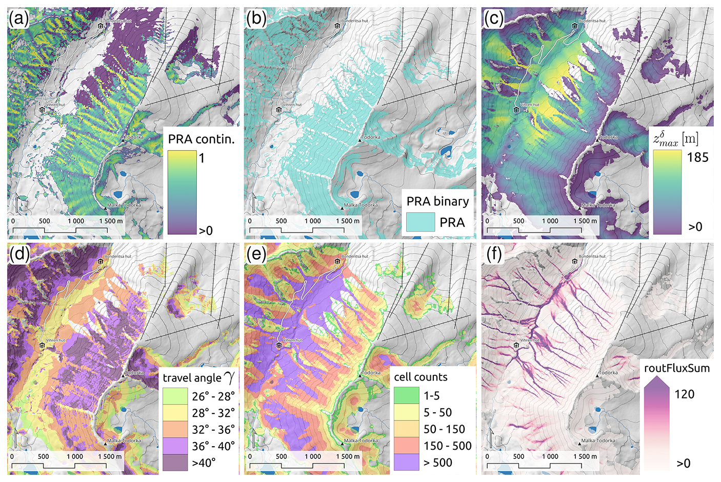
Figure A1Outputs of the PRA model (a, b) and avalanche runout modelling with com4FlowPy (c–f). (a) Continuous PRAs PRAcont, (b) binary PRAs PRAbin obtained with a threshold of 0.3, (c) maximum modelled energy line height , (d) maximum local travel angle (γ), (e) cell counts, and (f) sum of routing flux (∑routFlux).
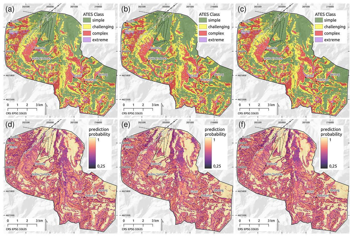
Figure A2ATES maps produced by the investigated RF models for the entire study area: (a) RF1, (b) RF2, and (c) RF3. Additionally, prediction probabilities output by the models for the ATES class prediciton: (d) RF1, (e) RF2, and (f) RF3.
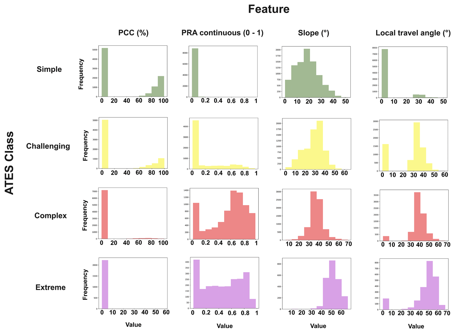
Figure A3Distributions of input feature values for pixels in the training data, grouped by ATES class. PCC stands for percent canopy cover, while PRA represents the potential release areas as a continuous raster, where 0 denotes no possibility of avalanche release, and 1 corresponds to a very high likelihood of release.
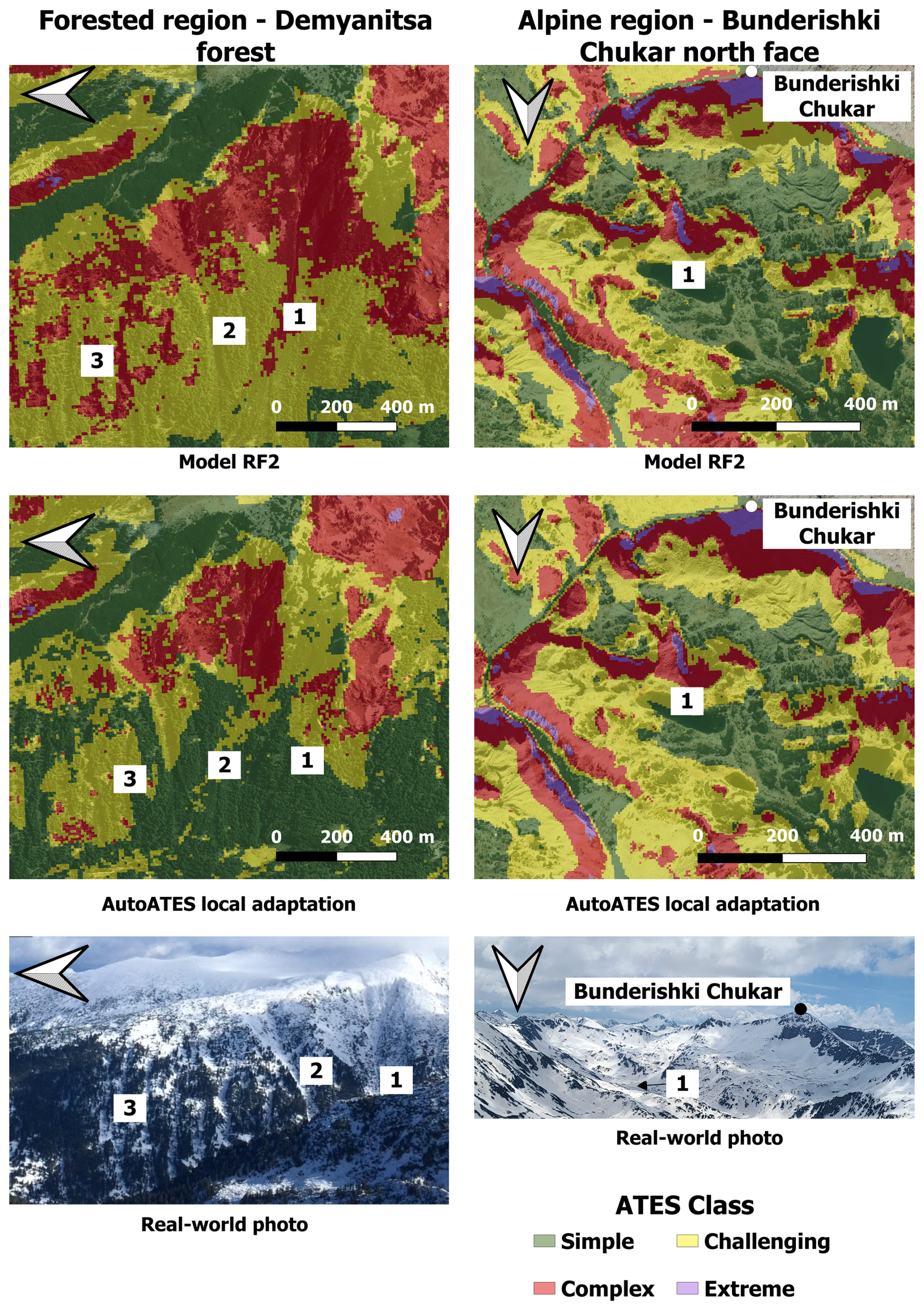
Figure A4Exemplary extract of the ATES map from model RF2 and the previous local adaptation of AutoATES in the study area (Panayotov et al., 2024b) for two separate areas – a sparsely forested region in Demyanitsa valley and the northern face of Bunderishki Chukar peak, part of the Bunderitsa valley, along with photographs of the winter terrain. The numbers highlight the corresponding terrain features between the photographs and the ATES predictions.
Table A1Distribution of ATES classes for the entire study region for the model RF2 and for the previous local adaptation of AutoATES in the study area (Panayotov et al., 2024b). The numbers represent the areas classified as each class in km2. The relative share of each class as a percent of the total area in % is provided in brackets.
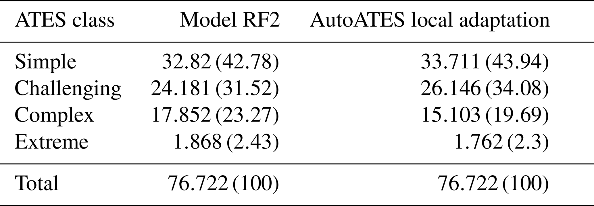
Table A2Feature importances for the RF1 model (trained on the original training dataset) and the model trained on the balanced forest vs. non-forest dataset (RF1 balanced).
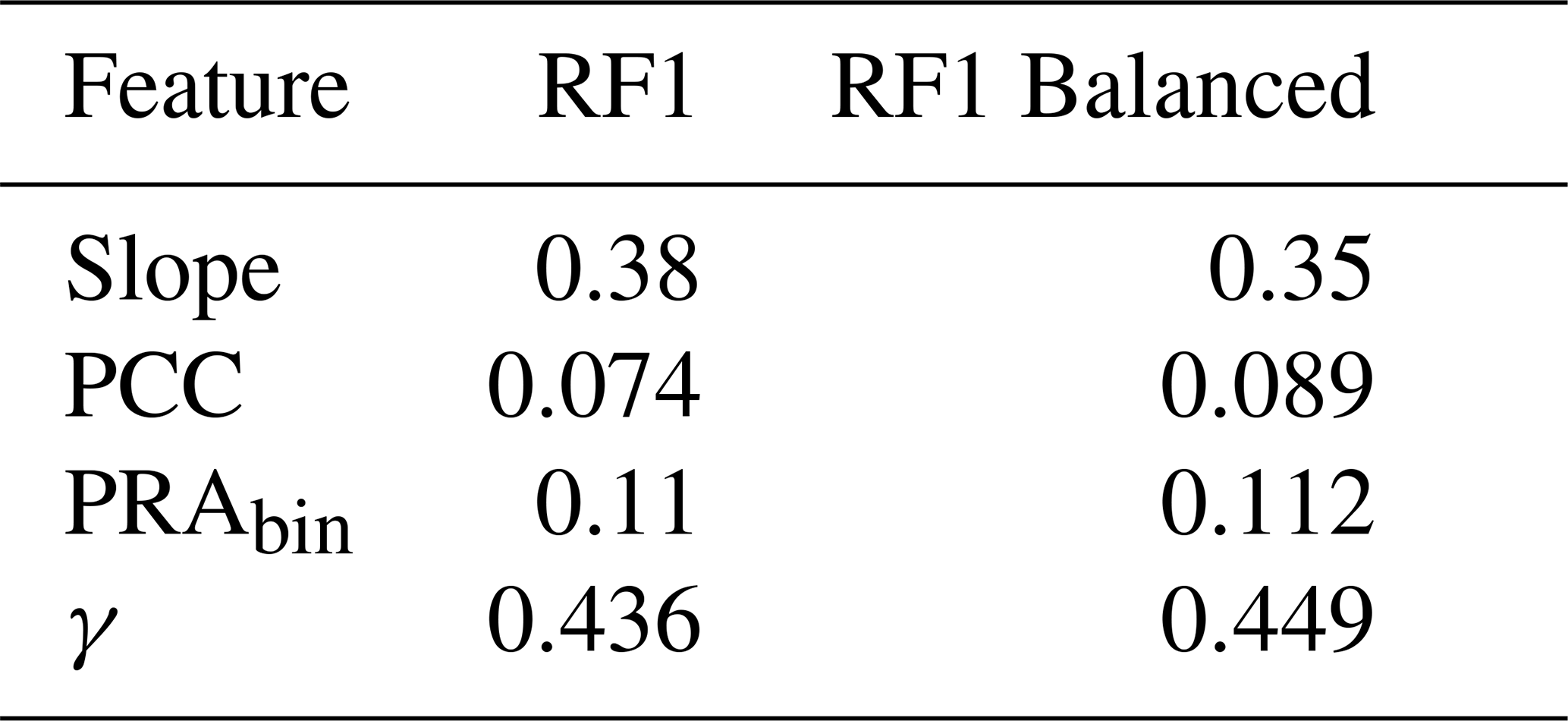
All Python code and trained model files can be found in our online Git repository: https://doi.org/10.5281/zenodo.15310357 (Markov, 2025). For future work, the GitHub repository: https://github.com/kalinmarkov95/machine-learning-auto-ates/tree/main (last access: 31 March 2025) will be maintained (Markov, 2025). Please refer to the repository for updates and potential additional data uploads.
The digital terrain model (DTM) of the study region was obtained from Pirin National Park and the private geospatial data provider Geopolyomorphic Cloud specifically for this study. It is not available for public use and is not included in the Git repository. If you would like to access the DTM, please contact the corresponding author, Kalin Markov (kmarkov@geophys.bas.bg), or the data providers directly (contact for Geopolymorphic Cloud: office@geopolymorphic-cloud.org; contact for Pirin National Park: dnp@pirin.bg).
KM: conceptualization, methodology, software, formal analysis, visualization, and writing – original draft preparation. AH: data curation, methodology, investigation, visualization, and writing – original draft preparation. MP, CH, PS, JTF, and MT: writing – review and editing. MP and MT: supervision, project administration, and funding acquisition.
The contact author has declared that none of the authors has any competing interests.
Publisher's note: Copernicus Publications remains neutral with regard to jurisdictional claims made in the text, published maps, institutional affiliations, or any other geographical representation in this paper. While Copernicus Publications makes every effort to include appropriate place names, the final responsibility lies with the authors. Views expressed in the text are those of the authors and do not necessarily reflect the views of the publisher.
The study was conducted as part of the project “Modelling of avalanches in forested and alpine terrain in Bulgaria and Austria – similarities and differences” funded by the National Science Fund of Bulgaria (Project KP-06-Austria/4/2023) and the Austrian Agency for International Cooperation in Education and Research OeAD (Project number BG 01/2023). Additional financial support was provided through the Open Avalanche Framework AvaFrame (https://www.avaframe.org, last access: 15 April 2025), a cooperation between the Austrian Research Centre for Forests (Bundesforschungszentrum für Wald; BFW) and the Austrian Service for Torrent and Avalanche Control (WLV), under the auspices of the Austrian Federal Ministry of Agriculture and Forestry, Climate and Environmental Protection, Regions and Water Management (BMLUK), as well as the Interreg Alpine Space project MOSAIC, co-funded by the European Union (grant number ASP0100014) and Multilateral Academic Projects (MAPS) of the Swiss National Science Foundation and the Bulgarian Ministry of Education grant IZ11Z0_230113. We would like to acknowledge the use of the Copernicus Tree Cover Density product. DTM data from Pirin National Park and Geopolymorphic Cloud were obtained for the needs of project KP-06-N31-3/2019 “Avalanche-forest interactions in the Pirin Mountains, Bulgaria” and also for a project supported by the Bulgarian Extreme and FreeSkiing Association (BEFSA). We acknowledge the use of AI tools that assisted in improving the readability in parts of the initial version of this manuscript.
This research has been supported by the Bulgarian National Science Fund (grant no. KP-06-Austria/4/2023), the OeAD-GmbH (grant no. BG 01/2023), Multilateral Academic Projects (MAPS) of the Swiss National Science Foundation, and the Bulgarian Ministry of Education and Science grant IZ11Z0_230113.
This paper was edited by Erich Peitzsch and reviewed by John Sykes and Cameron Campbell.
Acharya, A., Steiner, J. F., Walizada, K. M., Ali, S., Zakir, Z. H., Caiserman, A., and Watanabe, T.: Review article: Snow and ice avalanches in high mountain Asia – scientific, local and indigenous knowledge, Nat. Hazards Earth Syst. Sci., 23, 2569–2592, https://doi.org/10.5194/nhess-23-2569-2023, 2023. a
Afendras, G. and Markatou, M.: Optimality of training/test size and resampling effectiveness in cross-validation, Journal of Statistical Planning and Inference, 199, https://doi.org/10.1016/j.jspi.2018.07.005, 2019. a
Ahsan, M., Khan, A., Khan, K. R., Sinha, B. B., and Sharma, A.: Advancements in medical diagnosis and treatment through machine learning: a review, Expert Syst., 41, e13499, https://doi.org/10.1111/exsy.13499, 2024. a
Amin, G., Imtiaz, I., Haroon, E., Saqib, N. U., Shahzad, M. I., and Nazeer, M.: Assessment of machine learning algorithms for land cover classification in a complex mountainous landscape, Journal of Geovisualization and Spatial Analysis, 8, 34, https://doi.org/10.1007/s41651-024-00195-z, 2024. a
Bakkehøi, S., Domaas, U., and Lied, K.: Calculation of snow avalanche runout distance, Ann. Glaciol., 4, 24–29, https://doi.org/10.3189/S0260305500005188, 1983. a
Bhattacharyya, S.: Confidence in predictions from random tree ensembles, in: 2011 IEEE 11th International Conference on Data Mining, iSSN 2374–8486, https://doi.org/10.1109/ICDM.2011.41, 71–80, 2011. a
Bischl, B., Binder, M., Lang, M., Pielok, T., Richter, J., Coors, S., Thomas, J., Ullmann, T., Becker, M., Boulesteix, A.-L., Deng, D., and Lindauer, M.: Hyperparameter optimization: foundations, algorithms, best practices, and open challenges, WIREs Data Mining and Knowledge Discovery, 13, e1484, https://doi.org/10.1002/widm.1484, 2023. a
Breiman, L.: Random forests, Mach. Learn., 45, 5–32, https://doi.org/10.1023/A:1010933404324, 2001. a, b, c
Bühler, Y., Kumar, S., Veitinger, J., Christen, M., Stoffel, A., and Snehmani: Automated identification of potential snow avalanche release areas based on digital elevation models, Nat. Hazards Earth Syst. Sci., 13, 1321–1335, https://doi.org/10.5194/nhess-13-1321-2013, 2013. a, b
Bühler, Y., von Rickenbach, D., Stoffel, A., Margreth, S., Stoffel, L., and Christen, M.: Automated snow avalanche release area delineation – validation of existing algorithms and proposition of a new object-based approach for large-scale hazard indication mapping, Nat. Hazards Earth Syst. Sci., 18, 3235–3251, https://doi.org/10.5194/nhess-18-3235-2018, 2018. a, b
Campbell, C. and Gould, B.: A proposed practical model for zoning with the avalanche terrain exposure scale, in: Proceedings, International Snow Science Workshop 2013, Grenoble, France, https://arc.lib.montana.edu/snow-science/objects/ISSW13_paper_P5-02.pdf (last access: 1 April 2025), 2013. a
Cetinkaya, S. and Kocaman, S.: IMPACT OF LEARNING SET AND SAMPLING FOR SNOW AVALANCHE SUSCEPTIBILITY MAPPING WITH RANDOM FOREST, Int. Arch. Photogramm. Remote Sens. Spatial Inf. Sci., XLVIII-M-1-2023, 57–64, https://doi.org/10.5194/isprs-archives-XLVIII-M-1-2023-57-2023, 2023. a
Contreras, P., Orellana-Alvear, J., Muñoz, P., Bendix, J., and Célleri, R.: Influence of random forest hyperparameterization on short-term runoff forecasting in an Andean mountain catchment, Atmosphere-Basel, 12, 238, https://doi.org/10.3390/atmos12020238, 2021. a, b
Copernicus: Tree Cover Density 2018 (raster 10 m and 100 m), Europe, 3-yearly, European Environment Agency (EEA) [data set], https://doi.org/10.2909/486f77da-d605-423e-93a9-680760ab6791, 2020. a
D'Amboise, C., Teich, M., Hormes, A., Steger, S., and Berger, F.: Modeling protective forests for gravitational natural hazards and how it relates to risk-based decision support tools, in: Protective Forests as Ecosystem-based Solution for Disaster Risk Reduction (ECO-DRR), IntechOpen, London, https://doi.org/10.5772/intechopen.99510, 2021. a, b
D'Amboise, C. J. L., Neuhauser, M., Teich, M., Huber, A., Kofler, A., Perzl, F., Fromm, R., Kleemayr, K., and Fischer, J.-T.: Flow-Py v1.0: a customizable, open-source simulation tool to estimate runout and intensity of gravitational mass flows, Geosci. Model Dev., 15, 2423–2439, https://doi.org/10.5194/gmd-15-2423-2022, 2022. a, b, c, d, e
Dankan Gowda, V., Pathak, D., Prasad, K. D. V., Srinivas, V., Manu, Y. M., and Sudhakar Reddy, N.: Scalable machine learning frameworks for large-scale multimodal image and speech signal processing, in: 2024 8th International Conference on I-SMAC (IoT in Social, Mobile, Analytics and Cloud) (I-SMAC), ISSN 2768-0673, https://doi.org/10.1109/I-SMAC61858.2024.10714812, 1693–1699, 2024. a
Dutta, S., Arunachalam, A., and Misailovic, S.: To seed or not to seed? An empirical analysis of usage of seeds for testing in machine learning projects, in: 2022 IEEE Conference on Software Testing, Verification and Validation (ICST), IEEE, Valencia, Spain, https://doi.org/10.1109/ICST53961.2022.00026, 151–161, 2022. a
Engeset, R. V., Pfuhl, G., Landrø, M., Mannberg, A., and Hetland, A.: Communicating public avalanche warnings – what works?, Nat. Hazards Earth Syst. Sci., 18, 2537–2559, https://doi.org/10.5194/nhess-18-2537-2018, 2018. a
Gavaldã, J., Moner, I., and Bacardit, M.: Integrating the ATES into the avalanche information in Aran Valley (Central Pyrenees), in: Proceedings, International Snow Science Workshop 2013, Grenoble, France, https://arc.lib.montana.edu/snow-science/objects/ISSW13_paper_P5-01.pdf (1 May 2025), 2013. a
Gong, Y., Liu, G., Xue, Y., Li, R., and Meng, L.: A survey on dataset quality in machine learning, Inform. Software Tech., 162, https://doi.org/10.1016/j.infsof.2023.107268, 2023. a
Harvey, S., Schmudlach, G., Bühler, Y., Dürr, L., Stoffel, A., and Christen, M.: Avalanche terrain maps for backcountry skiing in Switzerland, in: Proceedings, International Snow Science Workshop, Innsbruck, Austria, Innsbruck, Austria, 1625–1631, https://arc.lib.montana.edu/snow-science/objects/ISSW2018_O19.1.pdf (last access: 12 February 2025), 2018. a
Harvey, S., Christen, M., Bühler, Y., Hänni, C., Boos, N., and Bernegger, B.: Refined Swiss avalanche terrain mapping CATV2/ATHV2, in: Proceedings, International Snow Science Workshop, Tromsø, Norway, 2024, Tromsø, Norway, 1637–1644, https://arc.lib.montana.edu/snow-science/item/3363 (last access: 17 April 2025), 2024. a
Hesselbach, C.: Adaptation and Application of an Automated Avalanche Terrain Classification in Austria, Master's thesis, University of Natural Resources and Life Sciences, Vienna, https://permalink.obvsg.at/bok/AC16964320 (last access: 22 April 2025), 2023. a, b, c
Horn, B. K. P.: Hillshading and the reflectance map, P. IEEE, 69, 14–47, https://doi.org/10.1109/proc.1981.11918, 1981. a
Huber, A., Hesselbach, C., Oesterle, F., Neuhauser, M., Adams, M., Plörer, M., Stephan, L., Toft, H., Sykes, J., Mitterer, C., and Fischer, J.-T.: AutoATES Austria – testing and application of an automated model-chain for avalanche terrain classification in the Austrian Alps, in: Proceedings, International Snow Science Workshop, Bend, OR, USA, 2023, Innsbruck, Austria, 1272–1278, http://arc.lib.montana.edu/snow-science/item/2989 (last access: 16 March 2025), 2023. a, b, c, d, e, f, g, h, i
Huber, A., Saxer, L., Spannring, P., Hesselbach, C., Neuhauser, M., D'Amboise, C., and Teich, M.: Regional-scale avalanche modeling with com4FlowPy – potential and limitations for considering avalanche-forest interaction along the avalanche track, in: Proceedings, International Snow Science Workshop, Tromsø, Norway, 2024, 587–594, https://arc.lib.montana.edu/snow-science/item.php?id=3194 (last access: 10 February 2025), 2024. a, b, c, d
Jaiswal, J. K. and Samikannu, R.: Application of random forest algorithm on feature subset selection and classification and regression, in: World Congress on Computing and Communication Technologies (WCCCT), https://doi.org/10.1109/wccct.2016.25, 2017. a
Japkowicz, N.: Concept-learning in the presence of between-class and within-class imbalances, in: Advances in Artificial Intelligence, edited by: Stroulia, E. and Matwin, S., Springer, Berlin, Heidelberg, https://doi.org/10.1007/3-540-45153-6_7, 67–77, 2001. a
Joseph, V. R.: Optimal ratio for data splitting, Statistical Analysis and Data Mining: The ASA Data Science Journal, 15, 531–538, https://doi.org/10.1002/sam.11583, 2022. a
Körner, H. J.: The energy-line method in the mechanics of avalanches, J. Glaciol., 26, 501–505, https://doi.org/10.3189/S0022143000011023, 1980. a
Larsen, H. T., Hendrikx, J., Slåtten, M. S., and Engeset, R. V.: Developing nationwide avalanche terrain maps for Norway, Nat. Hazards, 103, 2829–2847, https://doi.org/10.1007/s11069-020-04104-7, 2020. a, b, c, d, e, f, g, h
Markov, K.: kalinmarkov95/machine-learning-auto-ates: Implement Random Forest (RF) for automated ATES classification, Zenodo [code], https://doi.org/10.5281/zenodo.15310357, 2025. a, b
Markov, K. and Ivanov, I.: Avalanche Hazard Assessment and Modeling in Pirin National Park, LOPS Foundation, Sofia, Bulgaria, https://lopsbg.com/wp-content/uploads/2021/09/%D0%9A%D0%B0%D0%BB%D0%B8%D0%BD-%D0%9C%D0%B0%D1%80%D0%BA%D0%BE%D0%B2_%D0%98%D0%B2%D0%B0%D0%BD-%D0%98%D0%B2%D0%B0%D0%BD%D0%BE%D0%B2.pdf (last access: 30 March 2025), 2021. a
Markov, K. and Panayotov, M.: Defining of avalanche terrain with ATES modelling for the region of Bansko Ski Resort in Pirin, in: Avalanches in the Bunderitsa valley in Pirin Mountains, Intel Entrans, Sofia, ISBN 978-619-7703-60-3, 2024. a, b
Markov, K., Panayotov, M., Tcherkezova, E., and Teich, M.: Identifying and mapping avalanche terrain using the ATES model for the region around Bansko Ski Resort, Pirin, Forest Science (Nauka za Gorata), 60, 99–122, 2024. a
Markov, K., Panayotov, M., Tcherkezova, E., and Huber, A.: Influence of forest canopy cover on automated Avalanche Terrain Exposure Scale classification in the Pirin Mountains, Bulgaria, Forestry Ideas, 31, 170–187, https://forestry-ideas.info/issues/issues_Download.php?download=557 (last access: 30 October 2025), 2025. a
McClung, D. and Gauer, P.: Maximum frontal speeds, alpha angles and deposit volumes of flowing snow avalanches, Cold Reg. Sci. Technol., 153, 78–85, https://doi.org/10.1016/j.coldregions.2018.04.009, 2018. a
Nasteski, V.: An overview of the supervised machine learning methods, Horizons, 4, 51–62, https://www.researchgate.net/publication/328146111_An_overview_of_the_supervised_machine_learning_methods (last access: 29 October 2025), 2017. a, b
Oesterle, F., Wirbel, A., Fischer, J.-T., Huber, A., and Spannring, P.: avaframe/AvaFrame: 1.11, Zenodo [code], https://doi.org/10.5281/zenodo.14893015, 2025. a
Panayotov, M. and Tsvetanov, N.: Dating of avalanches in Pirin mountains in Bulgaria by tree-ring analysis of Pinus peuce and Pinus heldriechii trees, Dendrochronologia, 85, 126206, https://doi.org/10.1016/j.dendro.2024.126206, 2024. a
Panayotov, M., Menteshev, B., and Mihaylova, S.: Avalanches in Bulgaria, BEFSA, ISBN 978-619-188-515-2, 2021. a, b, c
Panayotov, M., Christen, M., Bebi, P., and Bartelt, P.: Simulation of avalanches in Bunderitsa valley with the RAMMS software, in: Avalanches in the Bunderitsa valley in Pirin Mountains, Intel Entrans, Sofia, ISBN 978-619-7703-60-3, 2024a. a
Panayotov, M., Markov, K., Tsvetanov, N., Huber, A., Hesselbach, C., and Teich, M.: Avalanche hazard mapping using the avalanche terrain exposure scale (ATES) in the high mountain ranges of Bulgaria, in: Proceedings, International Snow Science Workshop 2024, Tromsø, Norway, https://arc.lib.montana.edu/snow-science/objects/ISSW2024_P12.5.pdf (last access: 21 April 2025), 2024b. a, b, c, d, e, f, g, h, i, j, k, l, m, n, o, p, q, r
Pandey, S., Chand, S., Horkoff, J., Staron, M., Ochodek, M., and Durisic, D.: Design pattern recognition: a study of large language models, Empir. Softw. Eng., 30, https://doi.org/10.1007/s10664-025-10625-1, 2025. a
Parks Canada Agency: Avalanche Terrain Exposure Scale – Avalanche Terrain Exposure Scale, Government of Canada, https://parks.canada.ca/pn-np/bc/glacier/visit/hiver-winter/ski/ates (last access: 29 October 2025), 2017. a
Pedregosa, F., Varoquaux, G., Gramfort, A., Michel, V., Thirion, B., Grisel, O., Blondel, M., Prettenhofer, P., Weiss, R., Dubourg, V., Vanderplas, J., Passos, A., Cournapeau, D., Brucher, M., Perrot, M., and Duchesnay, E.: Scikit-learn: machine learning in Python, J. Mach. Learn. Res, 12, 2825–2830, 2011. a
Pirin National Park: Pirin National Park – World Heritage Property of Unesco, https://www.pirin.bg/?p=5591#more-5591 (last access: 28 August 2025), 2022. a, b
Prasetiyowati, M. I., Maulidevi, N. U., and Surendro, K.: Determining threshold value on information gain feature selection to increase speed and prediction accuracy of random forest, Journal of Big Data, 8, 84, https://doi.org/10.1186/s40537-021-00472-4, 2021. a
Probst, P., Wright, M., and Boulesteix, A.-L.: Hyperparameters and tuning strategies for random forest, WIREs Data Mining and Knowledge Discovery, 9, e1301, https://doi.org/10.1002/widm.1301, 2019. a, b
Pugliese, R., Regondi, S., and Marini, R.: Machine learning-based approach: global trends, research directions, and regulatory standpoints, Data Science and Management, 4, 19–29, https://doi.org/10.1016/j.dsm.2021.12.002, 2021. a
Python Software Foundation: Python Language Reference, version 3.9.21 [code], https://www.python.org/ (last access: 22 March 2025), 2024. a
Rainio, O., Teuho, J., and Klén, R.: Evaluation metrics and statistical tests for machine learning, Sci. Rep.-UK, 14, 6086, https://doi.org/10.1038/s41598-024-56706-x, 2024. a, b, c
Ramadhan, M., Sitanggang, I., Nasution, F., and Ghifari, A.: Parameter tuning in random forest based on grid search method for gender classification based on voice frequency, DEStech Transactions on Computer Science and Engineering, https://doi.org/10.12783/dtcse/cece2017/14611, 2017. a
Rimal, Y., Sharma, N., and Alsadoon, A.: The accuracy of machine learning models relies on hyperparameter tuning: student result classification using random forest, randomized search, grid search, bayesian, genetic, and optuna algorithms, Multimed. Tools Appl., 83, 74349–74364, https://doi.org/10.1007/s11042-024-18426-2, 2024. a
Rogers, J. and Gunn, S.: Identifying feature relevance using a random forest, in: SLSFS: International Statistical and Optimization Perspectives Workshop “Subspace, Latent Structure and Feature Selection”, edited by: Saunders, C., Grobelnik, M., Gunn, S., and Shawe-Taylor, J., Springer, Berlin, Heidelberg, https://doi.org/10.1007/11752790_12, 173–184, 2006. a
Salman, H. A., Kalakech, A., and Steiti, A.: Random forest algorithm overview, Babylonian Journal of Machine Learning, 2024, 69–79, https://doi.org/10.58496/BJML/2024/007, 2024. a, b
Saraswat, P.: Supervised machine learning algorithm: a review of classification techniques, Smart Innovation, Systems and Technologies, 273, 477–482, https://doi.org/10.1007/978-3-030-92905-3_58, 2022. a
Sarker, I. H.: Machine learning: algorithms, real-world applications and research directions, SN Computer Science, 2, 160, https://doi.org/10.1007/s42979-021-00592-x, 2021. a
Schmudlach, G. and Köhler, J.: Method for an automatized avalanche terrain classification, in: Proceedings, International Snow Science Workshop, Breckenridge, Colorado, 2016, Breckenridge, Colorado, 729–736, https://arc.lib.montana.edu/snow-science/objects/ISSW16_P2.04.pdf (last access: 7 April 2025), 2016. a
Schumacher, J., Toft, H., McLean, J. P., Hauglin, M., Astrup, R., and Breidenbach, J.: The utility of forest attribute maps for automated Avalanche Terrain Exposure Scale (ATES) modelling, Scand. J. Forest Res., 37, 264–275, https://doi.org/10.1080/02827581.2022.2096921, 2022. a, b, c, d, e
Schweizer, J. and Lüschg, M.: Characteristics of human-triggered avalanches, Cold Reg. Sci. Technol., 33, 147–162, https://doi.org/10.1016/S0165-232X(01)00037-4, 2001. a
Schweizer, J., Bartelt, P., and van Herwijnen, A.: Snow avalanches in: Snow and Ice-Related Hazards, Risks and Disasters, Elsevier, https://doi.org/10.1016/b978-0-12-394849-6.00012-3, 395–436, 2015. a
Sharp, A. E. A.: Evaluating the exposure of heliskiing ski guides to avalanche terrain using a fuzzy logic avalanche susceptibility model, Masters' thesis, University of Leeds, School of Geography, https://doi.org/10.13140/RG.2.2.18673.94567, 2018. a
Sharp, E., Campbell, C., Statham, G., and Schroers, B.: A standardized, multiscale, fuzzy spatialdata model for a Avalanche Terrain Exposure Scale mapping, in: Proceedings, International Snow Science Workshop, Bend, Oregon, 2023, 838–845, http://arc.lib.montana.edu/snow-science/item/2974 (last access: 5 April 2025), 2023. a
Siji George, G. C. and Sumathi, B.: Grid search tuning of hyperparameters in random forest classifier for customer feedback sentiment prediction, International Journal of Advanced Computer Science and Applications, 11, https://doi.org/10.14569/IJACSA.2020.0110920, 2020. a
Spannring, P.: Comparison of two avalanche terrain classification approaches: Avalanche Terrain Exposure Scale – Classified Avalanche Terrain, Master's thesis, University of Innsbruck, Faculty of Geo- and Atmospheric Sciences, https://resolver.obvsg.at/urn:nbn:at:at-ubi:1-155858 (last access: 30 October 2025), 2024. a
Statham, G. and Campbell, C.: The Avalanche Terrain Exposure Scale (ATES) v.2, Nat. Hazards Earth Syst. Sci., 25, 1113–1137, https://doi.org/10.5194/nhess-25-1113-2025, 2025. a, b, c, d, e, f
Statham, G., McMahon, B., and Tomm, I.: The Avalanche Terrain Exposure Scale, in: Proceedings, International Snow Science Workshop 2006, Telluride, Colorado, https://arc.lib.montana.edu/snow-science/objects/issw-2006-491-497.pdf (last access: 5 May 2025), 2006. a, b, c
Sykes, J., Toft, H., Haegeli, P., and Statham, G.: Automated Avalanche Terrain Exposure Scale (ATES) mapping – local validation and optimization in western Canada, Nat. Hazards Earth Syst. Sci., 24, 947–971, https://doi.org/10.5194/nhess-24-947-2024, 2024. a, b, c, d, e, f, g, h, i, j, k, l, m, n, o, p, q
Techel, F. and Zweifel, B.: Recreational avalanche accidents in Switzerland: trends and patterns with an emphasis on burial, rescue methods and avalanche danger, in: Proceedings International Snow Science Workshop 2013, Grenoble, France, https://arc.lib.montana.edu/snow-science/item.php?id=1844 (last access: 4 April 2025), 2013. a
Techel, F., Jarry, F., Kronthaler, G., Mitterer, S., Nairz, P., Pavšek, M., Valt, M., and Darms, G.: Avalanche fatalities in the European Alps: long-term trends and statistics, Geogr. Helv., 71, 147–159, https://doi.org/10.5194/gh-71-147-2016, 2016. a
Toft, H. B., Sykes, J., Schauer, A., Hendrikx, J., and Hetland, A.: AutoATES v2.0: Automated Avalanche Terrain Exposure Scale mapping, Nat. Hazards Earth Syst. Sci., 24, 1779–1793, https://doi.org/10.5194/nhess-24-1779-2024, 2024. a, b, c, d, e, f, g, h, i, j, k, l, m, n, o, p, q, r, s, t, u, v, w, x, y
Tonnel, M., Wirbel, A., Oesterle, F., and Fischer, J.-T.: AvaFrame com1DFA (v1.3): a thickness-integrated computational avalanche module – theory, numerics, and testing, Geosci. Model Dev., 16, 7013–7035, https://doi.org/10.5194/gmd-16-7013-2023, 2023. a
Tsvetanov, N. and Panayotov, M.: Dendrochronological reconstruction of large magnitude avalanches in Bunderitsa valley, in: Avalanches in the Bunderitsa valley in Pirin Mountains, Intel Entrans, Sofia, ISBN 978-619-7703-60-3, 2024. a, b
Ul Hassan, C. A., Khan, M. S., and Shah, M. A.: Comparison of machine learning algorithms in data classification, in: International Conference on Automation and Computing (ICAC), https://doi.org/10.23919/IConAC.2018.8748995, 2018. a
Varoquaux, G. and Colliot, O.: Evaluating machine learning models and their diagnostic value, in: Machine Learning for Brain Disorders, Springer US, ISBN 978-1-0716-3195-9, 2023. a, b, c
Veitinger, J., Purves, R. S., and Sovilla, B.: Potential slab avalanche release area identification from estimated winter terrain: a multi-scale, fuzzy logic approach, Nat. Hazards Earth Syst. Sci., 16, 2211–2225, https://doi.org/10.5194/nhess-16-2211-2016, 2016a. a, b
Veitinger, J., Sovilla, B., and Purves, R. S.: Model code of release area algorithm [code], https://github.com/jocha81/Avalanche-release (last access: 30 October 2025), 2016b. a, b
Venkadesh, P., S. V., D., Marymariyal, P., and Keerthana, S.: Predicting Natural Disasters With AI and Machine Learning, IGI Global Scientific Publishing, https://doi.org/10.4018/979-8-3693-3362-4.ch003, 2024. a
Viallon-Galinier, L., Hagenmuller, P., and Eckert, N.: Combining modelled snowpack stability with machine learning to predict avalanche activity, The Cryosphere, 17, 2245–2260, https://doi.org/10.5194/tc-17-2245-2023, 2023. a
von Avis, C. D., Sykes, J. M., and Tutt, B.: Development of large scale automated Avalanche Terrain Exposure Scale (ATES) ratings in collaboration with local avalanche experts, in: Proceedings, International Snow Science Workshop 2023, Bend, Oregon, 982–988, http://arc.lib.montana.edu/snow-science/item/2998 (last access: 12 April 2025), 2023. a, b
Wang, S., Zhuang, J., Zheng, J., Fan, H., Kong, J., and Zhan, J.: Application of Bayesian hyperparameter optimized random forest and XGBoost model for landslide susceptibility mapping, Front. Earth Sci., 9, https://doi.org/10.3389/feart.2021.712240, 2021. a
Werners, B.: Aggregation models in mathematical programming, in: Mathematical Models for Decision Support, Vol. 48 of NATO ASI Series, Springer, Berlin, Heidelberg, 295–305, https://doi.org/10.1007/978-3-642-83555-1_19, 1988. a
Yolanda, A., Adnan, A., Ell Goldameir, N., and Rizalde, F.: The comparison of accuracy on classification data with machine learning algorithms (case study: human development index by regency/city in Indonesia 2020), in: AIP Conference Proceedings, https://doi.org/10.1063/5.0118720, 2023. a