An ensemble random forest model for seismic energy forecasting

Seismic energy forecasting is critical for hazard preparedness, but current models have limits in accurately predicting seismic energy changes. This paper fills that gap by introducing a novel ensemble-based random forest framework for seismic energy forecasting. Building on a previously established methodology, the global energy time series is decomposed into intrinsic mode functions (IMFs) using ensemble empirical mode decomposition for better representation. Following this approach, we split the data into stationary (IMF₁) and non-stationary (sum of IMF₂–IMF₆) components for modelling. We acknowledge the inadequacy of IMFs in capturing seismic energy dynamics, notably in anticipating the final values of the time series. To overcome this limitation, the yearly seismic energy time series and the stationary and non-stationary parts are also fed as inputs to the developed models. In this study, we employ the support vector machine (SVM), random forest (RF), instance-based learning (IBk), ridge regression (RR), and multi-layer perceptron (MLP) algorithms for the modelling. Furthermore, the five models discussed above are suitably employed in a stacked regression ensemble using random forest as the meta-learner to arrive at the final predictions. The root mean squared error (RMSE) obtained in the training and testing phases of the validation model is 0.127 and 0.134, respectively. It is observed that the performance of the developed ensemble model is superior to those existing in the literature. Further, the developed algorithm is employed for the seismic energy prediction in the active Western Himalayan region for a comprehensively compiled catalogue, and the mean forecasted seismic energy for year 2024 is 7.21 × 10¹⁴ J. This work is a pilot project that aims to create a robust, scalable framework for forecasting seismic energy release globally and regionally. The findings of our investigation demonstrate the promise of the ensemble approach in delivering reliable seismic energy forecast, which can help with appropriate hazard preparedness.

1 Introduction

Earthquakes are among the most disastrous natural calamities due to the release of accumulated strain energy from continuous tectonic movements. Like other natural disasters, they can cause destruction both in financial terms and through loss of life (Jain, 2016). The devastating potential of earthquakes is increased by their fundamentally unpredictable character due to both aleatory and epistemic uncertainties (Kramer, 1996; Baker et al., 2021). Because the problem at hand is unpredictable, creating an accurate forecasting model is a unique challenge. There have been several attempts by seismologists to quantify the activity of regions based on several seismicity indicators. Some of the studies for the Himalayan region involved performing a palaeoseismic study (Lavé et al., 2005; Rajendran et al., 2013), using statistical inferences (Bilham and Ambraseys, 2005), taking Global Positioning System (GPS) measurements (Banerjee and Bürgmann, 2002; Ader et al., 2012), carrying out numerical calculations (Ismail-Zadeh et al., 2007; Jayalakshmi and Raghukanth, 2017), using satellite-imagery-based data (Bhattacharya et al., 2013; Misra et al., 2020), and performing Global Navigation Satellite System (GNSS) studies (Sharma et al., 2023b; Kumar et al., 2023a). However, the inadequacy in precisely monitoring stress changes, pressure, material variability, and temperature variation deep beneath the Earth's crust using scientific instruments leads to a lack of comprehensive data regarding accurate seismic characteristics. Subsequently, this lack of information has contributed to the uncertainty in earthquake occurrence, which has resulted in major risks to life and property. Hence, a robust quantification approach is essential considering the increasing vulnerability of the active regions due to developmental activities (Bilham, 2019). However, the variability in seismic behaviour, the worldwide occurrence of earthquakes, and the paucity of historical data all hamper predictive modelling. The ethical and practical consequences of delivering earthquake forecasts, the diversity in earthquake magnitudes, and the differences between human and geological timelines all add to the challenges in achieving reliable earthquake prediction (Mignan and Broccardo, 2020; Sun et al., 2022).

While progress is being made, the emphasis in earthquake research has turned toward establishing effective earthquake forecast models and early warning systems, understanding seismic risks, and improving preparation to lessen the effects of these deadly occurrences (Bose et al., 2008; Tiampo and Shcherbakov, 2012; Mousavi and Beroza, 2018; Mousavi et al., 2020; Tan et al., 2022). Nevertheless, with the advancements in field instrumentation, once an event occurs, we have attained the knowledge to estimate and record its information, like magnitude, location, extent of ground shaking, etc., immediately (USGS, 2024; IMD, 2024). The robustness of this data has also improved significantly over the years. An intriguing question here is as follows: is it possible to predict and be better prepared for a forthcoming event using this information? This study tackles this problem by compiling an extensive seismic dataset and building predictive models using state-of-the-art machine learning (ML) algorithms.

ML has evolved so much that its potential is widely explored to address numerous real-world problems (Schmidt et al., 2019; Kaushik et al., 2020; Sarker, 2021; Bertolini et al., 2021; Kumar et al., 2023b). Appropriate data processing using advanced ML algorithms has led to successful prediction models. However, ML algorithms have only recently gained popularity in engineering seismology (Xie et al., 2020; Mousavi and Beroza, 2023). The most comprehensive application is in developing efficient ground motion prediction equations (GMPEs) (Alavi and Gandomi, 2011; Derras et al., 2014; Dhanya and Raghukanth, 2018; Gade et al., 2021; Seo et al., 2022; Sreenath et al., 2024). Moreover, several machine learning techniques have been explored, among which multi-layer perceptrons (MLPs) are the most widely used model in earthquake engineering applications (Xie et al., 2020). Raghukanth et al. (2017) utilized a similar model for suitably combining stationary and non-stationary parts of energy series to forecast seismic energy. The MLP technique is also widely used in developing ground motion prediction equations, as evidenced by the works of Derras et al. (2014), Dhanya and Raghukanth (2018, 2020), and Douglas (2021). In another direction, Paolucci et al. (2018) proposed a simple MLP model that should efficiently generate broadband ground motions. Sharma et al. (2023a) improved the model by incorporating source, path, and site characteristics. Another architecture, i.e. linear regression (LR), has also been applied in various seismological studies due to its simplicity and efficiency. Pairojn and Wasinrat (2015) used LR for ground motion prediction in Thailand, while Cho et al. (2022) compared artificial neural networks (ANNs) and LR for predicting earthquake-induced slope displacement. The random forest (RF) technique has similarly motivated researchers across different fields, including seismology. Apart from the standard linear regression, studies have also used ridge regression for earthquake forecast problems (Ahmed et al., 2024). Pyakurel et al. (2023) utilized five supervised algorithms, including RF, to predict earthquake-induced landslides for the 2015 Gorkha earthquake. Additionally, Li and Goda (2023) extended the application of RF to tsunami early warning systems and loss forecasting. Furthermore, support vector machines (SVMs) with the optimized version named sequential minimal optimization for regression (SMOreg), as proposed by Shevade et al. (2000), are widely used for parameter learning. This approach has been applied to various natural hazard contexts, such as flood susceptibility mapping (Saha et al., 2021), ground motion prediction equations (Altay et al., 2023), and landslide monitoring (Kumar et al., 2023b). Similar to SMOreg, instance-based learning is also well explored in earthquake prediction problems, as its reliability and accuracy are owed to the algorithm's resistance to noise and outliers, as well as its versatility in the use of distance measures. Its applicability in seismic prediction is well demonstrated by Reyes et al. (2013), Ghaedi and Ibrahim (2017), Al Banna et al. (2020), and Ridzwan and Yusoff (2023).

Apart from the individual machine learning techniques, ensemble learning is a mature and widely adopted methodology in the ML literature, renowned for averaging several models to enhance prediction accuracy and generality (Dietterich, 2000; De Gooijer and Hyndman, 2006; Alpaydin, 2007). Ensemble models combine different base learners based on techniques such as bagging, boosting, and stacking and thus maximize the variance in data, reduce overfitting, and improve model reliability. They have been successful across a variety of applications, including medical diagnosis and climate modelling to financial forecasting (Re and Valentini, 2012; Tan et al., 2022; Rezaei et al., 2022). Although extensively used, their use in seismic energy forecasting is still not well exploited, making the current research a timely and new addition in the geophysical hazard field.

This research is based on the success of ensemble learning with the application of a stacked ensemble framework that is specific to the challenge of seismic energy forecasting. Even though ensemble models are extensively applied in other areas such as healthcare, climate, and finance, their niche use in seismic energy prediction remains limited and largely untapped. The predictions of five individual machine learning models – MLP, RF, LR, SMOreg, and instance-based learning with the parameter k (IBk) – are combined and stacked in this research through a random forest meta-learner. In this setup, the final ensemble model uses the random forest as a meta-learner that synthesizes predictions from these individual models, each trained using domain-informed design choices and preprocessing. As such, the RF model mimics a consensus-based expert system, combining diverse perspectives across learning paradigms to enhance forecasting robustness.

The improved long-term seismic energy prediction capability – essential for forward-looking hazard mitigation – is the main contribution of this work. The proposed model shows versatility across diverse tectonic environments by working well for both global and Western Himalayan datasets. The objective of this project is to apply stacked ensemble learning to develop a reliable model for annual seismic energy predictions. The empirical mode decomposition (EMD) method is applied to decompose global seismic energy time series, considering stationary and non-stationary components as inputs. The model is compared to existing research, and its predictive ability is established via a case study for the Western Himalayan region.

2 Global seismic energy (GSE) time series

Making accurate earthquake predictions requires a thorough earthquake catalogue. We have used two global earthquake catalogues for this study. Raghukanth et al. (2017) used the ISC-GEM catalogue (https://www.isc.ac.uk/, last access: 20 November 2024) as the primary resource. In the current study, the model construction, comparison, and validation of the suggested approach are done using this catalogue. A more thorough and current worldwide earthquake catalogue (up to 2023) was created using the USGS seismic database (https://earthquake.usgs.gov/earthquakes/search/, last access: 20 November 2024) and the ISC-GEM catalogue after the methodology was verified using these data. For our analysis, we used the same inputs as those mentioned in Raghukanth et al. (2017). We provide a brief explanation of the processing that goes into creating the final time series that is used for modelling in order to improve our understanding of the data. The validation catalogue, which is the worldwide earthquake catalogue that was obtained from Raghukanth et al. (2017), includes data from 1900 to 2015, totalling 24 375 occurrences with a minimum magnitude of M_w 4.98. The new global catalogue created for this study, which will be referred to simply as the global catalogue, is compiled from both USGS and ISC-GEM sources and contains data from 1900 to 2023. Duplicates were thoroughly examined and eliminated because the data were obtained from two distinct sources. There were 988 812 distinct occurrences with a minimum magnitude of 1.09 after duplicate events were removed. All reported event magnitudes were converted to moment magnitude (M_w) using empirical relationships from Scordilis (2006) and Yenier et al. (2008) to guarantee magnitude uniformity across datasets. We next determined the magnitude of completeness (M_c) for both catalogues, which is the lowest magnitude above which earthquakes are consistently documented. According to Raghukanth et al. (2017), using the maximum curvature approach (Wiemer and Wyss, 2000), M_c was determined to be 6.4 for the validation catalogue (Fig. S1a in the Supplement). Using the MATLAB-based program ZMAP version 7.1, M_c was calculated to be M_w 4.9 for the global catalogue, as seen in Fig. 1a.

Furthermore, the global catalogue's year of completeness was established using the Stepp (1973) approach, showing that the catalogue is complete starting in 1953 (Fig. 1b). Figure S1b and c display the distribution of events from the full validation catalogue (4619 events), while Fig. 1c shows the full global catalogue with 217 751 events. Because partial representation increases statistical bias, events with magnitudes < M_c were not included in the analysis. Furthermore, the energy contribution is dominated by large occurrences because the connection between seismic energy and earthquake magnitude is logarithmic. According to Eq. (1), for instance, the seismic energy associated with a M_w 3 event is 5.0596 × 10⁸ J, but the seismic energy associated with a M_w 5 event is 5.0596 × 10¹¹ J. This indicates that it takes roughly 1000 smaller M_w 3 events to equal the energy output of a single M_w 5 event. Therefore, from a hazard standpoint, smaller-magnitude events are not of major interest and do not considerably contribute to the total seismic energy. The 1960 M_w 9.6 Valdivia event is the greatest of the four major earthquakes (M_w ≥ 9) listed in the database. Instead of using monthly or weekly aggregation, which can result in deceptive zeros because of few occurrences in smaller windows, annual accumulation was employed to generate the seismic energy time series. Following Hanks and Kanamori (1979), moment magnitudes (M_w) were first transformed into seismic moments (M_o). Choy and Boatwright (1995) then estimated seismic energy (SE) using the relation:

$$\begin{array}{}\text{(1)}& \text{SE}=\mathrm{1.6}\times {\mathrm{10}}^{-\mathrm{5}}{M}_o,\text{where}{M}_o={\mathrm{10}}^{\mathrm{1.5}\times \left(M_{\mathrm{w}}+\mathrm{6}\right)}.\end{array}$$

For both catalogues, annual seismic energy time series were computed using this formula. Figure 2a for the global catalogue and Fig. S2a for the validation catalogue display the generated graphs. In the energy time history, significant occurrences like the earthquakes in Japan in 2011, Alaska in 1964, Sumatra in 2004, and Valdivia in 1960 emerge as peaks. The seismic energy was also presented in logarithmic form, as seen in Fig. 2b for the global catalogue and Fig. S2b for the validation catalogue, because sudden shifts in the time series can skew scale interpretation. The resulting time series is non-Gaussian and non-stationary, according to Raghukanth et al. (2017). As shown in the sections that follow, the signal was broken down into stationary and non-stationary components using ensemble empirical mode decomposition in order to better capture trends and cycles.

Figure 1 (a) Magnitude of completeness. (b) Year of completeness using the Stepp (1973) approach. (c) Distribution of the events from the complete global earthquake catalogue.

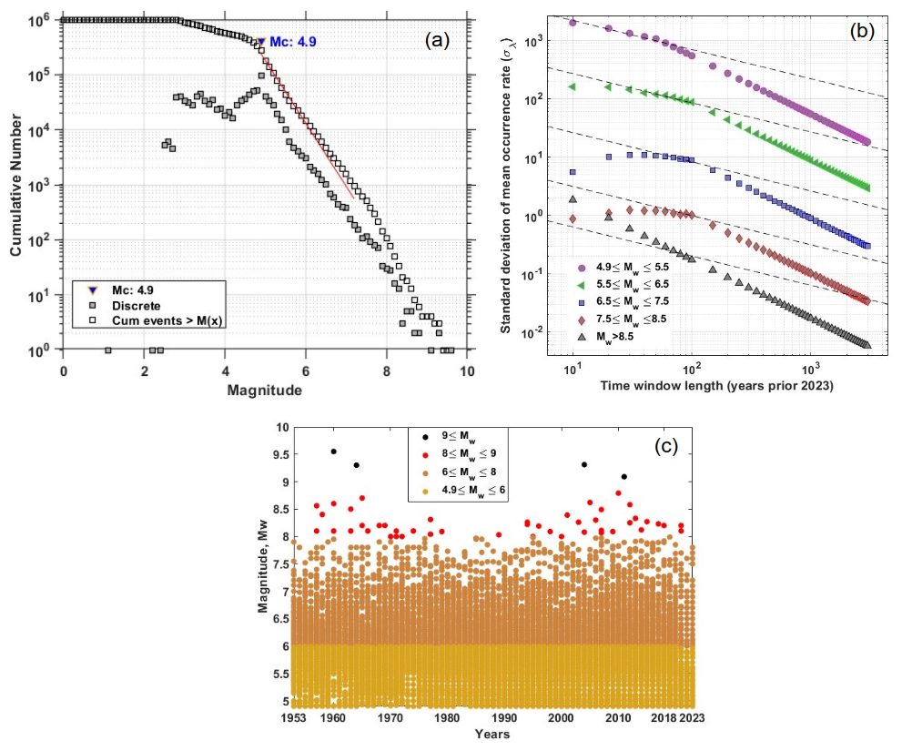
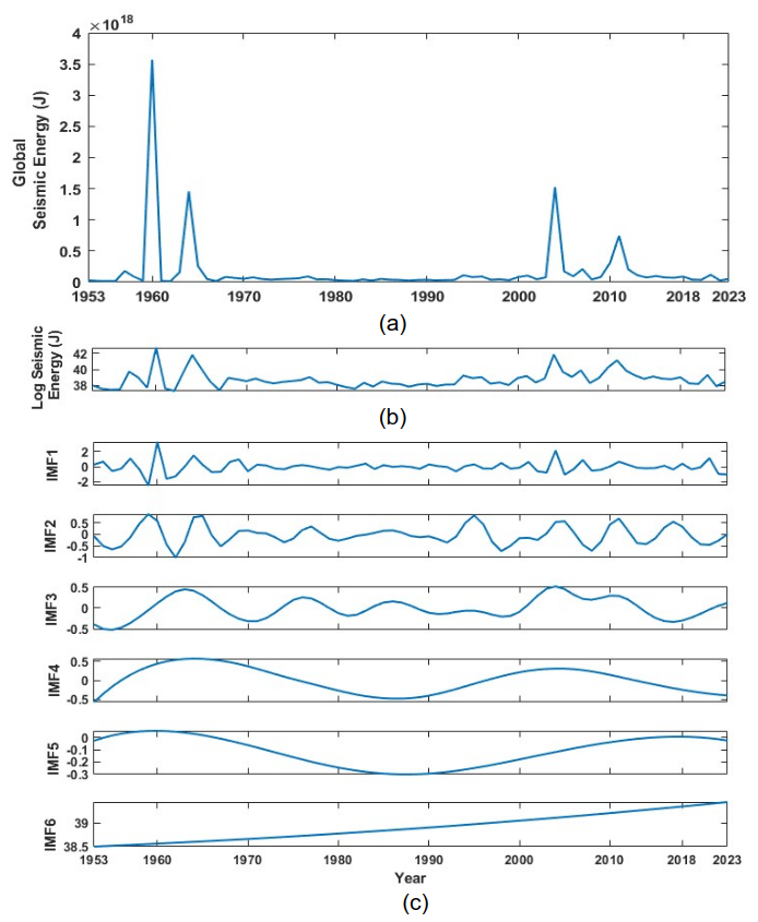
Figure 2 (a) Estimated global seismic energy (J) time series from the global catalogue used in developing the models. (b) Log-scaled global seismic energy time series (ln (GSE)). (c) Intrinsic modes estimated from ln(GSE) by performing ensemble empirical mode decomposition (EEMD).

2.1 Mode decomposition of GSE

The final seismic energy time series were split into orthogonal modes following the empirical mode decomposition (EMD) technique proposed by Huang et al. (1998). The basic functions, termed as intrinsic modes, were obtained following an iterative procedure on the data directly without any predefined functional form. Hence, the corresponding methodology is reported to be more adaptive to the features in the data. Furthermore, to avoid the issue of mode mixing in conventional EMD, Wu and Huang (2009) proposed ensemble EMD (EEMD), where finite white noise is added to the data while performing decomposition. The basic steps in the mode extraction involve (1) adding finite white noise to the data, (2) using a cubic spline to construct lower and upper envelopes connecting consecutive peaks as the respective sides, (3) estimating at each time step the average of positive and negative envelopes and then subtracting that from the data from step 1, (4) repeating steps 2–3 with the data from step 3 until we obtain the IMF (the time history where the number of extrema and the zero-crossing differ by one and the mean is zero), (5) subtracting the corresponding value from the time history in step 1 once the first IMF (IMF₁) is extracted, and (6) further following steps 2–4 to extract the next IMF. This is repeated until there are no zero-crossings left in the data. To perform ensemble empirical mode decomposition, steps 1–6 are repeated multiple times by adding different white noise, and the mean of IMFs at each level is identified as the final mode. The observations that served as the foundation for the above strategy are as follows: (1) if we take an average of white noise in a time domain, it cancels out in the ensemble mean. Hence, in the final noise-added ensemble signal, when averaged, only the signal survives, not the noise. (2) To drive the ensemble to exhaust all viable solutions, finite, not infinitesimal, amplitude white noise is required. Finite-magnitude noise causes the distinct scale signals to reside in the corresponding IMF, as mandated by the dyadic filter banks, and therefore improves the meaning of the final ensemble mean. For the data of the log seismic energy time series for the validation and global catalogues shown in Figs. S2b and 2b, we were able to extract six IMFs each following the described procedure. These IMFs are mostly uncorrelated and orthogonal. Also, for the physical interpretation of IMFs, various methods exist in the literature to estimate the periodicity of time series, including the instantaneous frequency method and Fourier-based approaches. The resulting IMFs in the present study are comparable to sine/cosine waves. Hence, counting the number of extremes in an IMF allows for easy estimation of the time period. Table 1 lists the periods of all six IMFs in log-scaled seismic energy time series from both catalogues. Table 1 also includes an estimate of the percentage variance for all IMFs, which is a statistical parameter, calculated as the ratio of the variance of each IMF to the variance of the data (Eq. 2). The %(variance) denotes the contribution of each IMF to annual earthquake energy release. It can be noted that IMF₁ constitutes the maximum variance of the time series and that IMF₆ represents the non-stationary trend in the data.

$$\begin{array}{}\text{(2)}& P_{{\mathrm{var}}_n}={\displaystyle \frac{\text{Var}\left(X_{{\mathrm{IMF}}_n}\right)}{\text{Var}\left(X_{\mathrm{data}}\right)}}\times \mathrm{100}\end{array}$$

Here, $P_{{\mathrm{var}}_n}$ is the % variance of the nth IMF.

Table 1 Period observed and the variance captured by the IMFs obtained for log-scaled seismic energy time series.

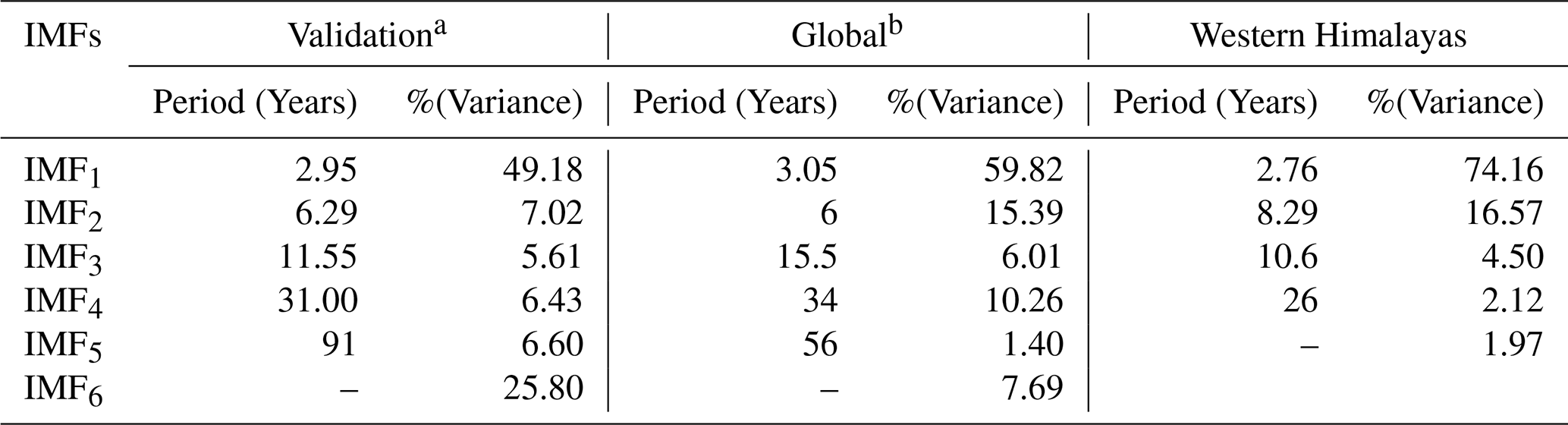
^a Validation catalogue is the catalogue sourced from Raghukanth et al. (2017).
^b Updated global catalogue prepared in the present study.

Moreover, the IMFs are simple and well behaved when compared to the original seismic energy data; hence, they can capture the physics of the occurrence of annual seismic energy when used as the input instead of complex seismic energy time series. Considering more about the physical interpretation of the IMF study performed by Liritzis and Tsapanos (1993), they calculated the periodicity of global shallow seismic events from conventional approaches like the Fourier method, and they determined the dominant periods to be 3(±0.5), 4.5, 6.5, 8–9, 14–20, and 31–34 years. IMF₁, being the predominant period, with a contribution of around 50 %–60 % to the annual seismic energy release, has a mean period of 3 years, which was also reported by Liritzis and Tsapanos (1993) as one of the periods. IMF₂ having a period in the range of 6 to 6.29 years also conforms with the period of 6.5 years reported by Liritzis and Tsapanos (1993). IMF₃, with a period ranging from 11 to 15.5 years, is in the range of the 11-year sunspot cycle reported by Raghukanth et al. (2017), who also found out that annual seismic energy release follows the sunspot period with a 2-year delay, and the standardized correlation coefficient between IMF₃ and the sunspot cycle is 0.3024, which is significant. IMF₄ and IMF₅ have 6 %–10 % and 1 %–6 % contributions to the annual seismic energy, respectively. Also, Wu and Huang (2004) proposed a methodology to assess the importance of IMFs by comparing them with the intrinsic mode functions of white noise. We performed the suggested test on the IMFs obtained by using the log seismic energy from the updated global catalogue, and the results are presented in Fig. 3. For pure noise, the energy and associated periods of IMFs will fluctuate linearly on the log–log plot, with all IMFs falling inside the confidence zone. It can be clearly inferred from Fig. 3 that all five IMFs (excluding IMF₆, which shows the trend) lie within the confidence interval, confirming that the IMFs are the signal. Hence, adopting the IMFs to forecast seismic energy instead of the complex seismic energy time series itself will better capture the underlying physics. For the forecast of seismic energy, autoregressive modes can be adopted. Thus, the linear and non-linear parts are separated, and IMF₁ is modelled separately from the remaining IMFs, as proposed by Iyengar and Raghukanth (2005) and Raghukanth et al. (2017). The corresponding IMF₁ to IMF₆ are shown in Fig. 2c for the global catalogue (corresponding figures for the validation catalogue are present in Fig. S2c and d). The correlation of the IMFs obtained by utilizing the log global time series of the global catalogue is shown in Fig. 4, from which it is evident that all the IMFs are almost orthogonal. In the present study, this information was suitably incorporated into more advanced machine learning algorithms to take one step ahead of the seismic energy forecast. A detailed description of the ML algorithms and the corresponding implementation is discussed further.

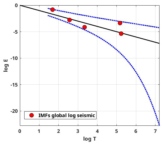
Figure 3 White noise test estimated using the procedure proposed by Wu and Huang (2004) for log seismic energy IMFs obtained from the global catalogue. The black line represents the expected line for white noise, and the dotted blue line shows the 95 % confidence band.

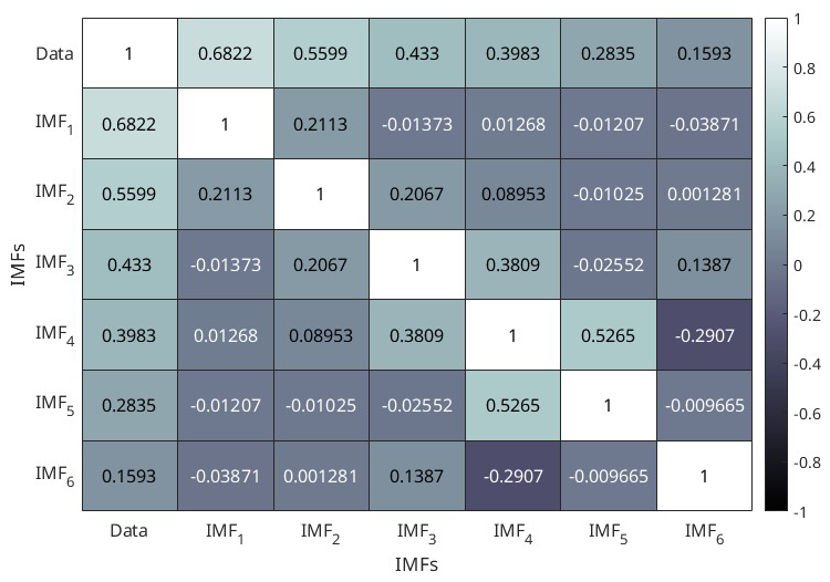
Figure 4 Correlation of the intrinsic mode functions obtained from the global seismic energy time series of global catalog.

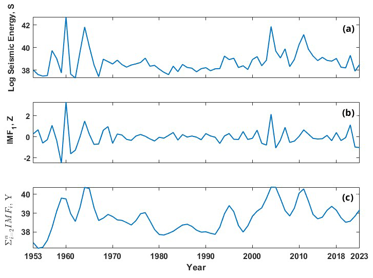
Figure 5 (a) Log-scaled global seismic energy time series (S) from the global catalogue, used as one of the inputs to the individual machine learning models. (b) First intrinsic mode function (Z) estimated from the log global seismic energy of the global catalogue, used as input to the individual models. (c) Summation of the second-to-last intrinsic mode functions obtained for the log global seismic energy of the global catalogue.

3 Methodology

There are numerous advanced machine learning techniques available in the literature. Some of the widely used variants include artificial neural networks (ANNs), decision trees, instance-based learning, classification, and regression models (Bishop, 2006). In this study, we attempted to include each of these flavours by including one representative algorithm for the analysis and further combining them using a suitable ensemble formulation. Furthermore, for seismic energy forecasting, four input parameters are employed, which are log seismic energy, i.e. the original time series data for log seismic energy, denoted as “S”; the first intrinsic mode function IMF1, denoted as “Z”; the sum of the remaining intrinsic mode functions, i.e. ${\sum }_{i=\mathrm{2}}^n{\text{IMF}}_i$, denoted as “Y”; and the year of occurrence of seismic energy. Furthermore, the description of each model utilized in the study is provided.

3.1 Multi-layer perceptron

The multi-layer perceptron (MLP) is part of an ANN (Bishop, 2006). A typical MLP architecture constitutes three layers, i.e. input, hidden, and output, mutually interconnected with weights. The typical functional form of an MLP from a single layer can be represented as

$$\begin{array}{}\text{(3)}& \widehat{y}=f\left(W\mathit{x}+b\right),\end{array}$$

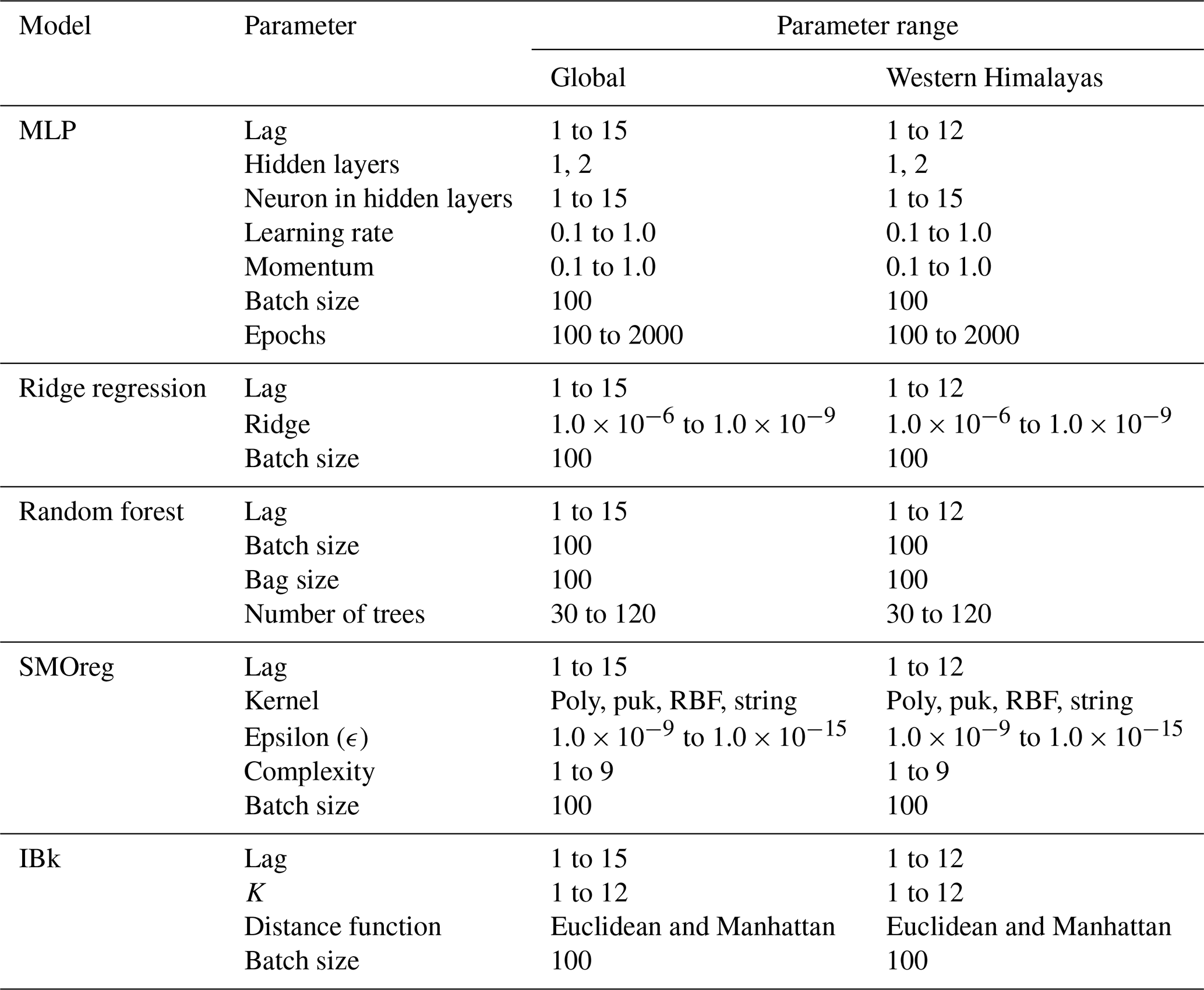
where $\widehat{y}$ is the output from the layer, f the activation function, W the weights, x the vector of inputs corresponding to the values at the previous layer, and b the bias. The number of hidden layers, nodes, and activation functions (e.g. linear, logistic, tanh, ReLU) depends on the non-linearity between predicted and predictor variables (Kumar et al., 2023b). Once the architecture is finalized, the parameters are estimated using back-propagation with the mean squared error (MSE) or mean absolute error (MAE) as the cost function. Our MLP uses four input features: log seismic energy (S), IMF1 (Z), ${\sum }_{i=\mathrm{2}}^n{\text{IMF}}_i$ (Y), and the year of occurrence of seismic energy. The hyperparameters for the model were optimized by varying the parameters as shown in Table 2. In time series forecasting, the concept of lag values is fundamental. Lag values refer to the number of past observations used to predict future values in a time series (Surakhi et al. 2021). By incorporating information from previous time points, models can capture temporal dependencies and trends, leading to more accurate forecasts. The lag values were varied from 1 to 15, the number of neurons in hidden layers from 1 to 15, the learning rate (L) from 0.1 to 1.0, momentum (M) from 0.1 to 1.0, and the number of epochs from 100 to 2000. A batch size of 100 was used for both the global and Himalayan models for consistency. For the Himalayan dataset (48 samples), this effectively resulted in full-batch training, which is appropriate given the small data size.

Table 2 Combinations considered for the optimization of hyperparameters in the model architecture.

3.2 Ridge regression (RR)

Ridge regression (RR) is one of the widely used statistical machine learning models (Hoerl and Kennard, 1970). It extends linear regression by introducing an L2 regularization term to penalize large coefficients, thereby improving generalization and reducing overfitting, especially in cases of multicollinearity or small datasets. The model establishes a linear relationship between the target variable and the input features, and the general form can be expressed as:

$$\begin{array}{}\text{(4)}& \widehat{y}={\mathit{\beta }}_{\mathrm{0}}+{\mathit{\beta }}_{\mathrm{1}}{x}_{\mathrm{1}}+{\mathit{\beta }}_{\mathrm{2}}{x}_{\mathrm{2}}+\mathrm{\dots }+{\mathit{\beta }}_n{x}_n+\mathit{ϵ},\end{array}$$

where y is the target variable, $\widehat{y}$ is the predicted value, $x_{\mathrm{1}},\mathrm{\dots },x_n$ are the input variables, β₀ is the intercept, ${\mathit{\beta }}_{\mathrm{1}},\mathrm{\dots },{\mathit{\beta }}_n$ are the regression coefficients, n is the number of features, p is the total number of data points, and ϵ is the error term.

In ridge regression, the coefficients β_i are estimated by minimizing a regularized loss function:

$$\begin{array}{}\text{(5)}& \underset{\mathit{\beta }}{min}\left\{\sum _{i=\mathrm{1}}^p{\left(y_i-{\widehat{y}}_i\right)}^{\mathrm{2}}+\mathit{\lambda }\sum _{j=\mathrm{1}}^n{\mathit{\beta }}_j^{\mathrm{2}}\right\}.\end{array}$$

Here, λ is the ridge regularization parameter that controls the strength of the penalty. The unknown parameters ${\mathit{\beta }}_{\mathrm{0}},\mathrm{\dots },{\mathit{\beta }}_n$ are estimated using the gradient descent algorithm with the mean squared error (MSE) as the cost function.

$$\begin{array}{}\text{(6)}& \text{MSE}={\displaystyle \frac{\mathrm{1}}{p}}\sum _{i=\mathrm{1}}^p{\left(y_i-{\widehat{y}}_i\right)}^{\mathrm{2}}\end{array}$$

Based on the number of input variables, there are two common variants of linear models: single-variable linear regression and multiple-variable linear regression.

RR architectures are employed for developing the forecast model. The inputs are the same as for the MLP. The lag values were varied from 1 to 15, which resulted in transformed input parameters from the higher order of the time variable and the product of time and different lagged variables. Attribute selection methods, such as the M5 method introduced by Quinlan (1992) and the Greedy method, can be used to reduce the number of attributes. In this work, the M5 method was used, retaining only the time steps from input variables that significantly affect the results for regression. The hyperparameter “ridge” was varied from 1.0 × 10⁻⁶ to 1.0 × 10⁻⁹, and the batch size was consistently set to 100, as shown in Table 2.

3.3 Random forest

Random forest (RF) is a supervised learning model used for classification and regression (Breiman, 2001). It combines multiple decision trees to improve predictive accuracy (Cutler et al., 2012). A decision tree has decision nodes (with branches) and leaf nodes (with no branches). Trees start from a root node containing the entire dataset, splitting at each node based on attribute selection measures (ASMs) like information gain or the Gini index. Pruning removes unnecessary nodes to prevent overfitting.

RF addresses overfitting by building multiple decision trees on different data subsets and averaging their predictions. This ensemble of uncorrelated trees uses bootstrap sampling and feature randomness. RFs have lower computational costs, handle missing data, and can manage larger datasets efficiently. Randomness in tree generation is controlled by a fixed seed (set to 1). The number of trees (iterations) was varied from 30 to 120, and tree depth is unlimited (depth of 0). Features at each split are calculated by (log ₂(N)+1), where N is the number of predictors (Breiman, 2001). The lag values were varied from 1 to 15, and the batch size and bag size were consistently set to 100, as shown in Table 2.

3.4 Sequential minimal optimization regression

Sequential minimal optimization (SMO) is an iterative algorithm proposed by Platt (1998) for solving regression problems using support vector machines (SVMs). SMO simplifies the optimization problem by breaking it down into smaller sub-problems that can be solved analytically, which makes it more efficient for training SVMs. Further improvements to SMO for regression were proposed by Shevade et al. (2000), who introduced modifications to enhance its efficiency. These improvements address the way SMO updates and maintains threshold values, resulting in two significantly more efficient versions for regression tasks. The corresponding algorithm effectively solves the quadratic optimization problem inherent in SVM training. SMOreg employs four input features: log seismic energy (S), IMF1 (Z), ${\sum }_{i=\mathrm{2}}^n{\text{IMF}}_i$ (Y), and the year of occurrence of seismic energy. The model is optimized by fine-tuning hyperparameters such as the complexity number (C) and epsilon (ϵ). In this study, the complexity number was varied from 1 to 9 to balance minimizing the training error and problem complexity. Epsilon was varied from 1.0 × 10⁻⁹ to 1.0 × 10⁻¹⁵ to determine the allowable error within the epsilon tube. The kernel function, crucial for SVMs, impacts the ability to manage complex relationships in the data. Various kernel functions, including polynomial (Polykernel), puk, RBF, and string kernels, were considered. The lag values were varied from 1 to 15, and the batch size was consistently set to 100, as shown in Table 2.

3.5 Instance-based learning with the parameter k

Instance-based learning (IBL), also called instance-based learning with the parameter k (IBk), is a type of supervised learning used for both classification and regression problems (Aha et al., 1991; Jo, 2021). It falls under lazy learning algorithms, which memorize the training data and make predictions based on the similarity between new and training datasets. The parameter k represents the number of nearest neighbours considered for predictions. IBk searches for the k most similar instances from the training dataset based on the similarity measures using the Manhattan distance, Euclidean distance, or other distance matrices. More accurately, let the given instance x be described by the feature vector $〈{\mathit{a}}_{\mathbf{1}}\mathbf{\left(}\mathit{x}\mathbf{\right)}\mathbf{,}{\mathit{a}}_{\mathbf{2}}\mathbf{\left(}\mathit{x}\mathbf{\right)}\mathbf{,}\mathbf{\dots }{\mathit{a}}_{\mathit{n}}\mathbf{\left(}\mathit{x}\mathbf{\right)}〉$, where a_r(x) denotes the value of the rth attribute of instance x. The Euclidean distance between x_i and x_j is given by

$$\begin{array}{}\text{(7)}& d(x_i,x_j)\equiv \sqrt{\sum _{r=\mathrm{1}}^n\left({\left(a_r\left(x_i\right)-a_r\left(x_j\right)\right)}^{\mathrm{2}}\right)}.\end{array}$$

Here, in the k-nearest neighbour algorithm, the target function may be either real-valued or discrete-valued, defined by $\widehat{f}\left(x_q\right)$, which is just the most common value of f among k training examples nearest to x_q.

$$\begin{array}{}\text{(8)}& \widehat{f}\leftarrow {\displaystyle \frac{{\sum }_{i=\mathrm{1}}^{k}f\left(x_i\right)}{k}}\end{array}$$

In this study, the k value was varied between 1 and 12, using Euclidean and Manhattan distances. The lag values were varied from 1 to 15, resulting in transformed input features. The number of nearest neighbours for prediction was set using these variations, with a consistent batch size of 100, as shown in Table 2. The LinearNNSearch algorithm, suitable for small datasets, was adopted for the nearest neighbour search, employing a linear search across all data points.

4 Ensemble models

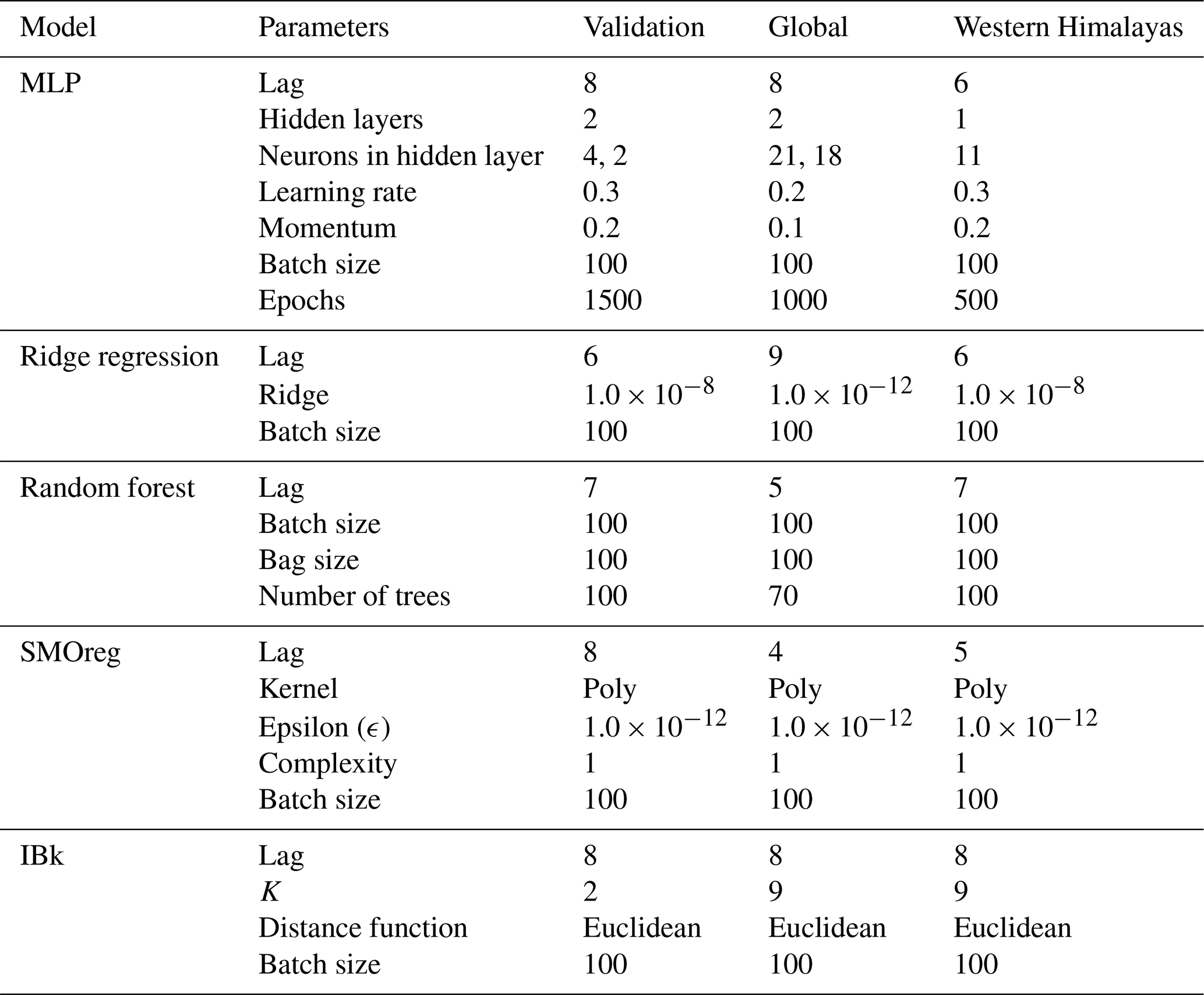
Hyndman and Athanasopoulos (2018) suggested that in time series forecasting approaches, there is a need to include relevant characteristics to increase accuracy. Also, the wider notion of adding time-related characteristics is a well-known approach in machine learning and forecasting. Hence, the inclusion of year as one of the input features is decided in the present study. Now, using only IMFs as the inputs for developing the forecasting model might not be that effective because finding IMF1 at the boundary of the data can be challenging due to undefined envelopes on both sides. To address this challenge, the previous value of the end point might be used as the next value. However, this strategy is not effective for anticipating issues. If n data are provided, IMFs can only be extracted for i = 2, 3, 4,$\mathrm{\dots },n-\mathrm{1}$. As the distance between extrema increases, extrapolation errors might permeate into the signal, misrepresenting greater IMFs at the end points. Hence, the inclusion of S in the input ensures that the deficiency of the empirical mode decomposition to estimate the end value does not affect the model predictions. Hence, the time histories from S, Y, and Z (see Fig. 5 for the global catalogue and Fig. S2 for the corresponding figure for the validation catalogue) were provided simultaneously as inputs to the model, along with the year, to predict S as the output variable. The time series up to 1995 is taken for the training phase and the remaining data from 1996–2015 are considered for the testing phase for the validation catalogue, whereas for the updated global catalogue, the time series up to 2009 is taken for training and 2009–2023 for testing. Additionally, the combination of the inputs is determined such that it gives the best prediction when performing beta coefficient analysis, whereby the approach tries different indices and retains only those that are significant and minimizes the prediction error. To determine the optimal lag period, an analysis was performed by varying the lag from 1 to 15 time points. The optimal lag value was identified by evaluating the model's performance and selecting the lag period that minimizes the prediction error. The range of lag values, along with the other hyperparameters varied to get the final model, is presented in Table 2. Also, different lag values for different models were obtained, and these values, along with the other hyperparameters used in the prediction models, are presented in Table 3. The overall flow of the proposed approach is described in Fig. 6. Furthermore, a detailed description of the model architectures of the ensemble model is furnished in Sect. 4.1.

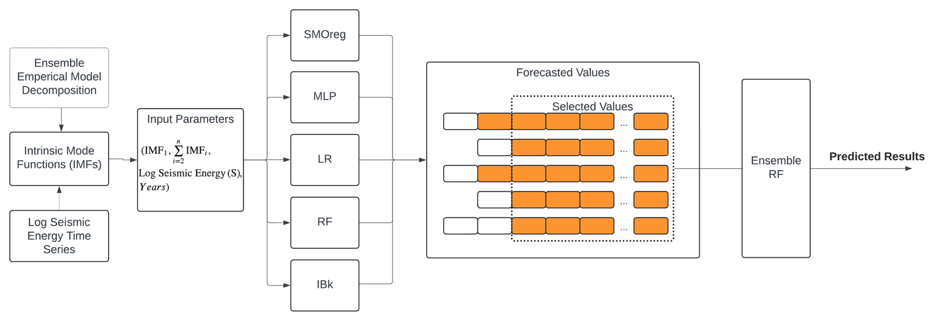
Figure 6 Flow chart representing the various steps and modelling approaches adopted for seismic energy forecasting.

Table 3 Optimized hyperparameter of the models for the data under consideration.

4.1 Ensemble model architecture

Ensembling can be performed by second-level trainable combiners through meta-learning techniques (Duin and Tax, 2000). In the present study, the stacking method was employed, wherein the output results of the base or weak learners were used as features in an intermediate space. These features were subsequently fed as input to a second-level meta-learner to perform a trained combination of weak learners. The base learners in this study included MLP, LR, RF, SMOreg, and IBk, which forecasted the values of seismic energy, as depicted in Fig. 6. These base learners were optimized models with varying parameters, as detailed in Table 2. Each base learner produced predictions of different lengths due to the use of varying lag values in their optimization process. To address this discrepancy and ensure consistency across all learners, the shortest prediction length among the models was used to align the inputs. This approach was visually represented in Fig. 6, where the orange blocks indicated the forecasted values and the empty blocks denoted absent values. Here, forecasted values from all five techniques were then used as input features for the ensemble RF model, with the actual log seismic energy as the target for regression. This ensemble RF model ultimately predicted the log seismic energy, integrating the results from the base learners to improve the ensemble prediction accuracy.

To ensure optimal performance of the models, we employed grid search techniques for hyperparameter tuning. Grid search is an exhaustive search method that tests all possible combinations of specified hyperparameters to identify the best-performing configuration for each model. The process involves defining a parameter grid for each model, specifying a range of values for each hyperparameter. For example, for the multi-layer perceptron (MLP), the grid includes different numbers of neurons in the hidden layers, learning rates, and momentum values. For the random forest (RF), the grid includes the number of trees and maximum depth. Each combination of hyperparameters is evaluated using an 80:20 train–test split method. The dataset is divided into 80 % training and 20 % testing sets, with the model trained on the training set and evaluated on the testing set. The performance of each hyperparameter combination is assessed using an appropriate evaluation metric, such as the mean squared error (MSE) or root mean squared error (RMSE). The combination of hyperparameters that results in the lowest error (or highest accuracy) on the training set is selected as the optimal configuration for the model. The final model, with optimized hyperparameters, is then tested on the testing dataset to evaluate its generalization performance. This ensures that the selected model configuration not only performs well on the training data but also maintains its accuracy, generalization, and robustness.

4.2 Input and output to different models

The proposed two-level ensemble forecasting framework operates on a structured input–output configuration where the input vector comprises four fundamental components: log seismic energy (S), IMF₁ (Z), ${\sum }_{i=\mathrm{2}}^n{\text{IMF}}_i$ (Y), and temporal information, i.e. the year of occurrence of seismic energy, systematically organized into sequential packets, i.e. ($X_{\mathrm{1}},X_{\mathrm{2}},\mathrm{\dots },X_m$) for training and ($X_{m+\mathrm{1}},\mathrm{\dots },X_n$) for testing, with a suitable temporal dependency structure (i.e. lag value). All four features (S, Z, Y, and year) have lagged values in each input packet, which are structured so that past observations are utilized to forecast future S values. A generalized flow of input and output is presented in Fig. 7 for a lag value of 8. However, different base models have different lag values. These lag values are determined based on the optimized model for varying parameters, as presented in Table 2. The final values of lag for different base learners are presented in Table 3. To be clear, the model is trained to predict the seismic energy at the subsequent time step (e.g. S9), and each input packet contains eight previous time steps of S, Y, Z, and year as features for a lag value of 8. This sliding-window method guarantees that the learning algorithm employs logical event sequences and catches temporal patterns in the data. The first level of the ensemble processes these input packets with different lag values through five different base models (linear regression, multi-layer perceptron, SMOreg, IBk, and random forest) that make the initial predictions. This changes the original four-dimensional input space into a five-dimensional prediction space, where each observation is represented by the outputs from all base models. After that, the second level uses a random forest meta-learner to process these stacked five-dimensional prediction vectors and make final consensus predictions (S₉, S₁₀, S₁₁, S₁₂, …, S_n). In order to ensure temporal consistency and assess prediction performance, the same input structure is employed during the testing phase by shifting the lag window across unseen sequences. To prevent input mismatches, the output from only the overlapping prediction region (shortest sequence) is sent to the meta-learner because each base learner employs a distinct lag length. This is done by using the collective intelligence of the base models and learning the best combination weights and interaction patterns to make better predictions than individual algorithmic approaches. This is done by systematically combining different temporal pattern recognition capabilities across different seismic conditions.

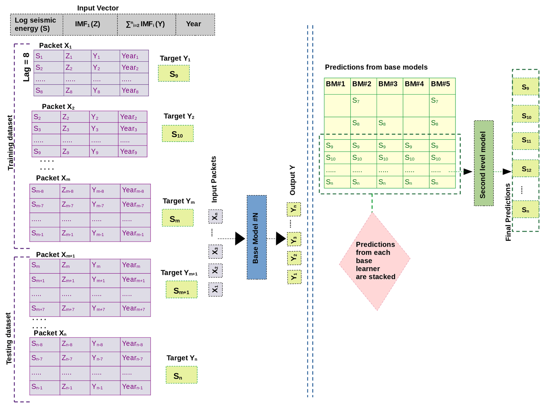
Figure 7 A general diagram showing the input and output at different stages of the methodology with a representative value of lag = 8.

5 Validation

Based on the optimized hyperparameters, the predictions from the models trained on the data derived from the validation and global catalogues in the training and testing phases are summarized in Figs. 8 and 9 for the individual models. The performance is observed to vary between models in both the training and testing parts. Hence, to have a quantitative evaluation of the model performances, the following indicators are estimated for both the training and testing phases:

1. Standard deviation of error (σ(ϵ))

   $$\begin{array}{}\text{(9)}& \mathit{\sigma }\left(\mathit{ϵ}\right)=\sqrt{{\displaystyle \frac{\sum _{i=\mathrm{1}}^N\left(S_i-{\widehat{S}}_i\right)-\stackrel{\mathrm{‾}}{\left(S_i-{\widehat{S}}_i\right)}}{N-\mathrm{1}}}}\end{array}$$

2. Pearson correlation coefficient (R)

   $$\begin{array}{}\text{(10)}& R={\displaystyle \frac{\sum _{i=\mathrm{1}}^N\left(S_i-\stackrel{\mathrm{‾}}{S_i}\right)\left({\widehat{S}}_i-\stackrel{\mathrm{‾}}{{\widehat{S}}_i}\right)}{\sqrt{\sum _{i=\mathrm{1}}^N{\left({\widehat{S}}_i-\stackrel{\mathrm{‾}}{{\widehat{S}}_i}\right)}^{\mathrm{2}}\sum _{i=\mathrm{1}}^N{\left(S_i-\stackrel{\mathrm{‾}}{S_i}\right)}^{\mathrm{2}}}}}\end{array}$$

3. Performance parameter (PP)

   $$\begin{array}{}\text{(11)}& \text{PP}=\mathrm{1}-{\displaystyle \frac{\langle \parallel S-\widehat{S}{\parallel }^{\mathrm{2}}\rangle }{{\mathit{\sigma }}_{\widehat{S}}^{\mathrm{2}}}}\end{array}$$

4. Root mean squared error (RMSE)

   $$\begin{array}{}\text{(12)}& \text{RMSE}=\sqrt{{\displaystyle \frac{\sum _{i=\mathrm{1}}^N{\left(S_i-{\widehat{S}}_i\right)}^{\mathrm{2}}}{N}}}\end{array}$$

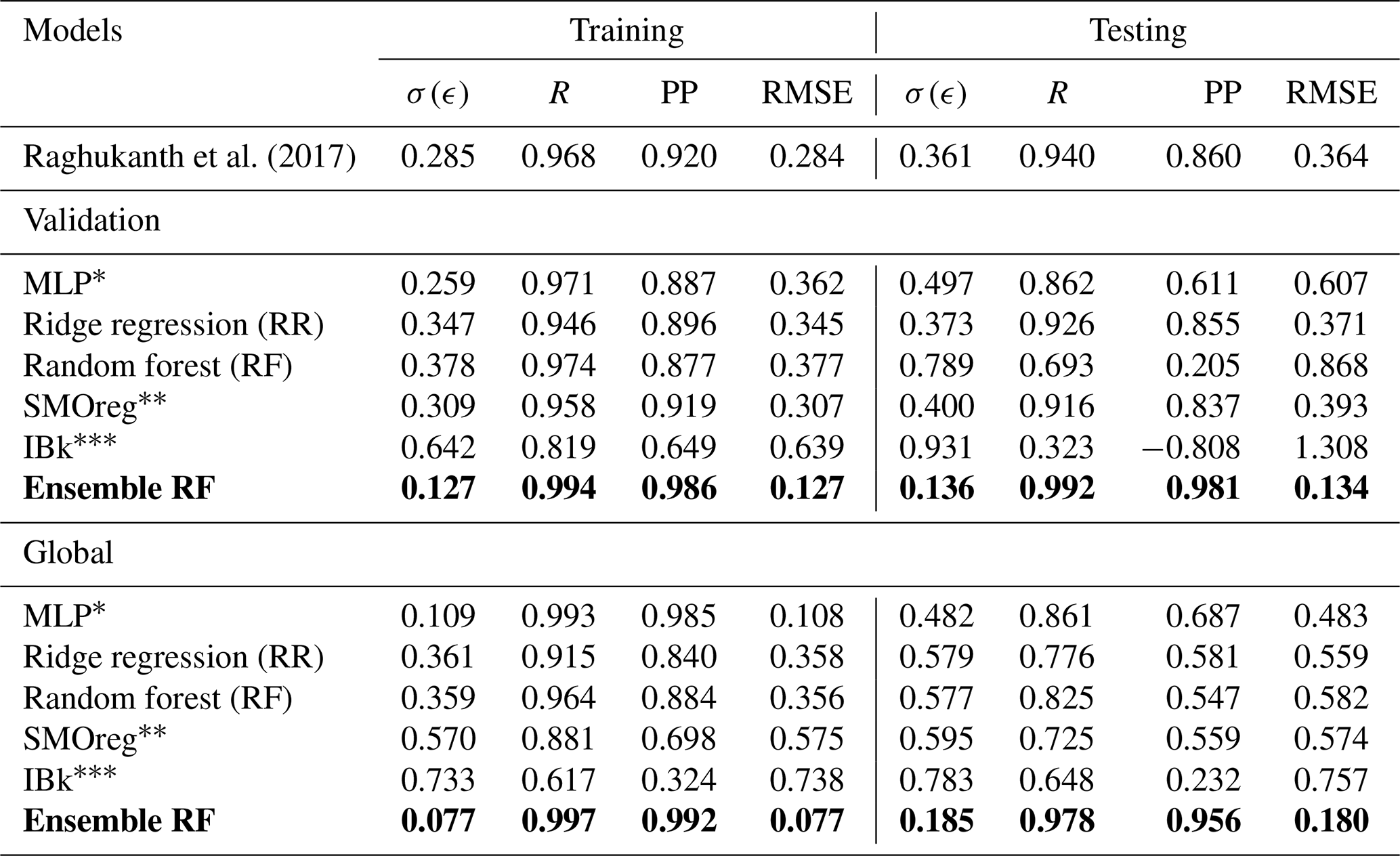
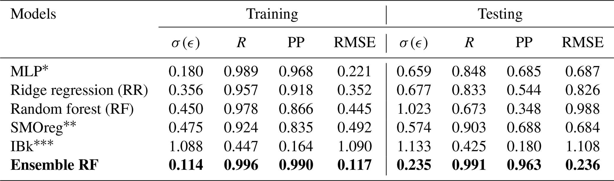
To ensure reliable model selection while mitigating overfitting, hyperparameter tuning is performed using the training dataset. This approach avoids information leakage from the testing set and ensures unbiased performance estimates. Rather than reserving a third dataset exclusively for validation, this strategy allows efficient use of the available data while maintaining a robust generalization capability. The final model performance is then evaluated on the separate hold-out test set. The corresponding estimations for the weak learners and ensemble models are summarized in Table 4. For models developed with the validation catalogue log seismic energy data, the MLP model performs well in the training phase; however, in the testing phase, it is relatively weak. By contrast, the MLP model developed on the global catalogue data performs well in both the training and testing phases. The RF model also shows a similar trend to that of MLP. However, the LR and SMOreg models are observed to perform consistently in both the training and testing phases. The IBk architecture is the worst-performing model for both the validation and global catalogues under consideration. Nevertheless, according to the detailed literature review explained earlier, ensemble models are expected to improve the model's performance. Thus, a suitable ensemble model is developed, as described in Sect. 4. The corresponding model performance is summarized in Fig. 10 for the validation catalogue and Fig. 11 for the global catalogue, as well as in Table 4. Interestingly, across both datasets, the ensemble model outperformed any single base learner in terms of the RMSE and correlation coefficients. Furthermore, the model performance is good and consistent in both the training and testing phases. Additionally, from a comparison of performance with the previous study (Raghukanth et al., 2017) (Table 4) on the same data, i.e. the validation catalogue, we were able to conclude that the ensemble model performs significantly better, having lesser variability. As a result, the relevant model may be a good fit for real-time seismic energy forecasting applications and can be appropriately used to produce accurate seismic energy predictions. With this motivation, we further attempt to explore the proposed approach for regional-level seismic energy forecasting. The active Western Himalayan province is chosen for the evaluations. A detailed description of the corresponding data, processing, and modelling is provided in Sect. 6.

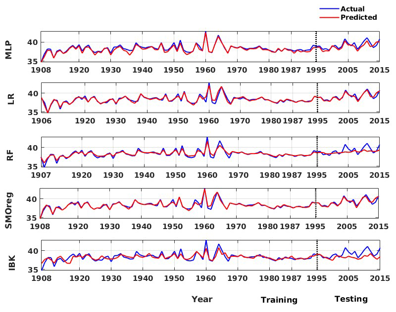
Figure 8 Actual vs. predicted values of global log seismic energy from individual machine learning techniques adopted in this work for the validation catalogue data.

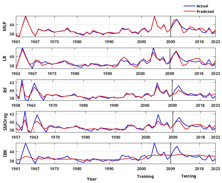
Figure 9 Actual vs. predicted values of individual machine learning techniques for global log seismic energy calculated from the global catalogue.

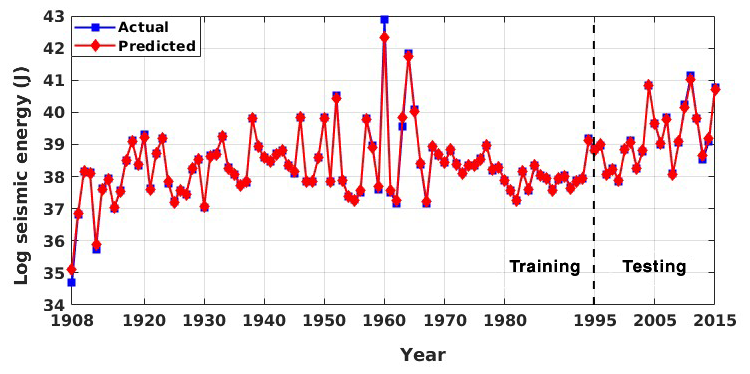
Figure 10 Actual vs. predicted values for global seismic energy from the proposed ensemble random forest model for the validation catalogue.

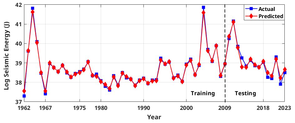
Figure 11 Actual vs. predicted values of the proposed ensemble random forest model for global log seismic energy calculated from the global catalogue.

Raghukanth et al. (2017)

Table 4 Performance evaluation of the individual models and the final ensemble random forest model (highlighted with the bold characters) in the training and testing phases for global seismic energy.

^* MLP – multi-layer perceptron.
${}^{**}$ SMOreg – sequential minimal optimization regression.
${}^{***}$ IBk – instance-based learning with the parameter k.

6 Application to Western Himalayas

The vast Indian subcontinent region, which includes Bangladesh, India, Nepal, Bhutan, Pakistan, and Sri Lanka, is prone to frequent and severe earthquakes. This region is particularly vulnerable to seismic activity because of the tectonic movements and the proximity to the convergent margin of the Indian and Eurasian plates. The subsequent collision has resulted in a vast mountain belt known as the Great Himalayas, where frequent earthquakes are caused by ongoing tectonic activity. The uplift due to collision has caused linear zones of deformation, leading to crustal shortening along major boundary faults. These faults are the Himalayan Frontal Thrust (HFT), Main Boundary Thrust (MBT), and Main Central Thrust (MCT), which have resulted in some large palaeo-earthquakes in the region (Dasgupta et al., 2000). India's northern and northeastern parts are more vulnerable; they are classified majorly as seismic zones IV and V in IS 1893-1 (2016), which indicates the highest degree of seismic hazard. As the Indian plate slowly sinks and subducts beneath Asia at a pace of around 47 mm yr⁻¹, this collision tectonics makes the area very vulnerable to catastrophic earthquakes due to energy accumulation and subsequent release (Bendick and Bilham, 2001). Several large earthquakes have been observed in this region in the last 2 decades, such as the Uttarkashi earthquake in 1991 (m_b 6.6), the Chamoli earthquake in 1999 (m_b 6.3), the Kashmir earthquake in 2005 (M_w 7.8), the Sikkim earthquake in 2011 (M_w 6.9), and the Nepal earthquake in 2015 (M_w 7.8). Moreover, the region between the Kangra earthquake in 1905 (M_w 7.8) and the Bihar-Nepal earthquake in 1934 (M_w 8) is relatively silent and hence is identified as the central seismic gap (CSG) region, having the potential to generate > 8 magnitude events (Bilham et al., 1997; Khattri, 1999; Bilham, 2019). It is therefore essential to have a reliable quantification of hazard in order to reduce the related seismic risks in the active Western Himalayan area. The current approach, designed especially for this seismically active and dynamic area, is critical. Its alignment with the distinct geological features of the Western Himalayas emphasizes its significance and makes it an indispensable instrument for reducing the possible effect of seismic occurrences in this susceptible region. Furthermore, seismic hazard studies have also reported high values for design parameters for the region due to its active tectonics and recurrence rate (NDMA, 2010; Nath and Thingbaijam, 2012; Dhanya and Raghukanth, 2022; Sreejaya et al., 2022). Considering the tectonics and the risk due to exposure, an efficient forecast model is critical for this region. However, a dedicated model for annual seismic energy forecasting is still lacking. Hence, the present work aims to develop a robust forecast model for annual seismic energy release in the Western Himalayas. The ensemble model algorithm validated in Sect. 5 shall be utilized for the work. A detailed description of the data compiled for the region and the resultant forecast is furnished. This application demonstrates the extension of our ensemble methodology to a regional scale with real hazard implications.

6.1 Study region and data preparation

From the tectonics described earlier, the Hindu Kush region and the adjoined region are seismically very active, as evident from Fig. 12. This observation is consistent with both the frequency of documented earthquakes and the geographical distribution of faults and lineaments (Fig. 12). This has motivated researchers to divide the whole geographical area of the country and the adjoining region into different seismic zones. For instance, Khattri et al. (1984) used seismotectonic and seismicity data to split the nation into 24 source zones. Bhatia et al. (1999) found 85 source zones in India, whereas 40 seismic zones were detected by another research Parvez et al. (2003). Considering all these past efforts, the National Disaster Management Authority (NDMA) of India created a thorough study in 2010 that further divided the whole Indian subcontinent into 32 seismic zones, designated SZ-1 to SZ-32 NDMA (2010). This division of seismic zones was done by considering factors such as regional geodynamics, fault alignment, and recurrence parameters for the regions. Among these 32 zones, the present study focuses on earthquakes in SZ-1, SZ-2, SZ-6, and SZ-30, which lie in the western part of the Himalayan belt. As this is preliminary work towards energy prediction for the regions, the comprehensive catalogue is combined together for all zones in the Western Himalayas. Here, the earthquake catalogue for the region has been taken from Dhanya et al. (2022) and was updated until 31 December 2023 via the USGS seismic database (https://earthquake.usgs.gov/earthquakes/search/, last access: 20 November 2024). There are 25 769 events (for the Western Himalayan region considered for this work) in the final updated catalogue, spanning from 1250 BCE to 2023 CE. Furthermore, the updated catalogue has been checked for both completeness for year and magnitude. For completeness of year, the method suggested by Stepp (1972) has been adopted, in which the standard deviation of the mean rate is plotted as a function of the sample length, and the period where this value deviated from the tangent, i.e. $\mathrm{1}/\sqrt{\left(T\right)}$, is considered as completeness for the considered magnitude. Furthermore, the magnitude of completeness is identified from the maximum curvature method proposed by Wiemer and Wyss (2000). The catalogue compiled for the region in the present work is observed to have a magnitude of completeness of M_w 4 and a corresponding year of completeness of 1964 (Fig. 13a and b). Hence, events spanning from 1964 and having a magnitude greater than M_w 4 have been considered for further input preparation. The distribution of the event in the final compiled catalogue can be identified from Fig. 14.

Figure 12 The regional-level tectonics and past seismicity, where the highlighted portion shows the seismogenic zones as per NDMA (2010) in the Western Himalayas.

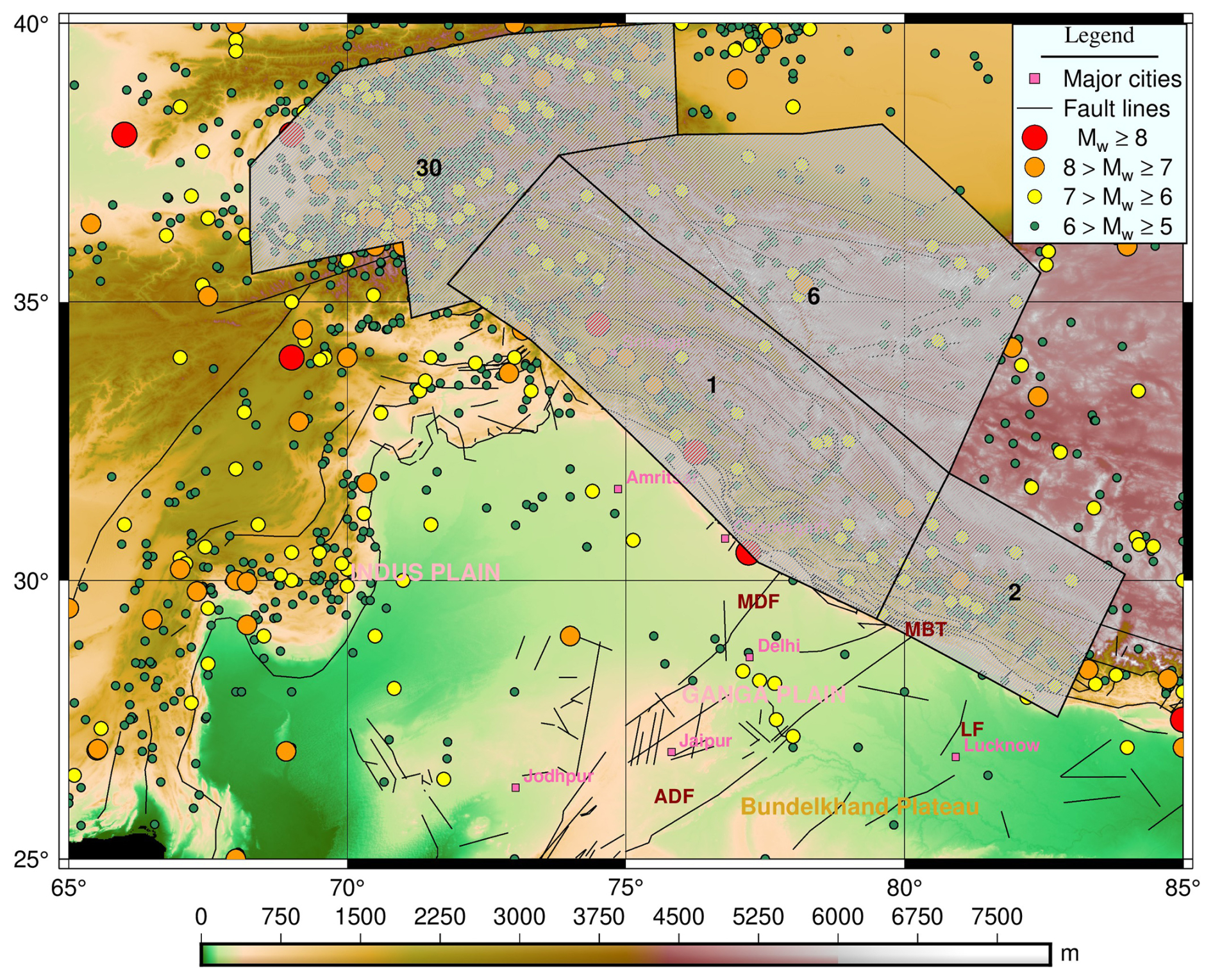
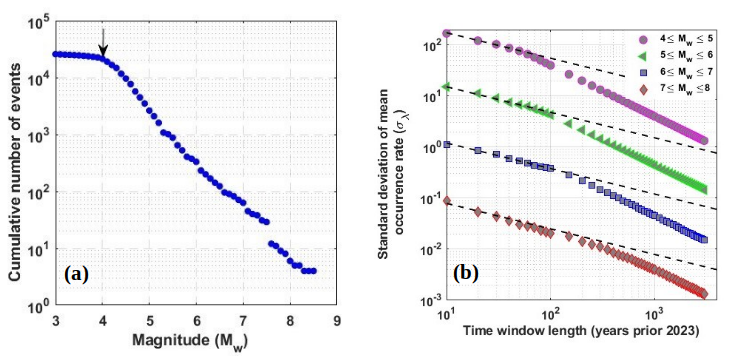
Figure 13 (a) The magnitude of completeness derived using the approach of Wiemer and Wyss (2000) and (b) the year of completeness derived using the approach of Stepp (1972), obtained for the catalogue compiled for the Western Himalayan region.

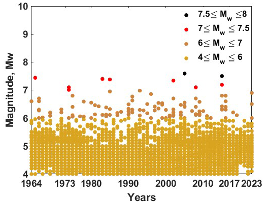
Figure 14 Distribution of events for the complete catalogue for the Western Himalayan region. Events with magnitude equal to or greater than M_w 7.5 are shown in black.

6.2 Seismic time series and mode decomposition

The same approach discussed in Sect. 2 has been adopted for the Western Himalayas, where the complete catalogue spanning from 1964 to 2023 with 20 774 events having a magnitude in different scales is unified by converting all the earthquake magnitudes into moment magnitudes M_w. The catalogue has two major earthquakes with a magnitude M_w ≥ 7.5: the 2005 Kashmir earthquake (M_w 7.6) and the 2015 Afghanistan earthquake (M_w 7.5) (Fig. 14). After unification, magnitudes are converted to seismic energy using Eq. (1) as discussed in Sect. 2, considering the physical significance of the parameter in earthquake occurrence. Furthermore, energies are added annually to get the seismic energy time series. From Fig. 15a, one can note two distinct peaks at 2005 and 2015, indicators of the major earthquakes explained earlier. Furthermore, to enhance the predictability of the time series, these values are converted to log scale to remove sudden jumps, similar to that described in Sect. 2. After the seismic energy time series is obtained, it is further decomposed into intrinsic mode functions using the EEMD technique. The corresponding division is expected to account for the linear and non-linear components of time histories appropriately. The decomposition allows the model to separately learn dominant cycles (IMF1) and low-frequency, non-linear patterns (IMF₂–IMF₅). Thus, by applying the EEMD technique as described in Sect. 2.1 on the log-scaled Western Himalayan seismic energy time series (Fig. 15b, first subplot), we are able to obtain five intrinsic mode functions (Fig. 15b). Furthermore, the correlation coefficients between the models are presented in Fig. 16. It is noted that the IMFs are mostly uncorrelated and orthogonal. Table 1 lists the periods and variance of all five IMFs in the log-scaled seismic energy time series. Similar to the global seismic energy modes, for the regional model, the period of the IMFs seems to increase. Furthermore, IMF₁ is observed to capture maximum variance in the data. To incorporate these IMFs as input for the machine learning techniques, IMF₁ and the sum of IMF₂ to IMF₅ (${\sum }_{i=\mathrm{2}}^{\mathrm{5}}{\text{IMF}}_i$) have been taken separately, as suggested in Raghukanth et al. (2017). Furthermore, considering the limitation of EEMD at the time series boundary, the log seismic energy and year are also used as model inputs (see Fig. 17). A detailed description of the model architecture that was found optimal for the regional database is discussed further.

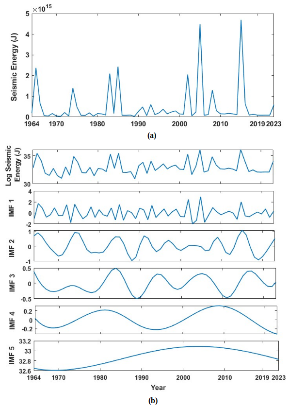
Figure 15 (a) Annual seismic energy estimated for the catalogue compiled for the Western Himalayas. (b) Log-scaled seismic energy for the Western Himalayas, and the corresponding intrinsic mode function obtained by employing ensemble empirical mode decomposition (EEMD).

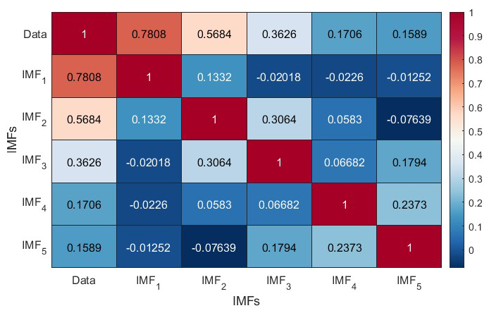
Figure 16 The correlation coefficient estimated for the intrinsic mode functions extracted from the log-scaled seismic energy time series of the Western Himalayas.

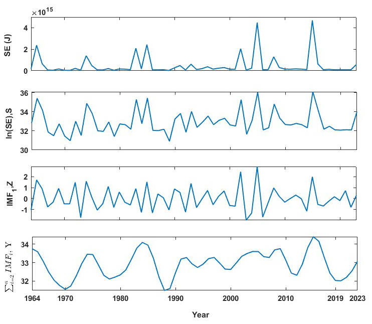
Figure 17 Estimated seismic energy series from the updated catalogue for the Western Himalayan region used in developing the models. (a) Global seismic energy (GSE) time series, with units of joules. (b) Log-scaled GSE. (c) First intrinsic mode estimated from ln (GSE) by performing ensemble empirical mode decomposition (EEMD). (d) Sum of the second to last intrinsic modes estimated from ln(GSE) by performing EEMD.

6.3 Model architecture for the Western Himalayas

After input preparation, the approaches discussed in Sect. 3 are also tested for the active Western Himalayan region, i.e. the obtained IMFs along with the log seismic energy and year of occurrence are taken as input for the first-level individual machine learning techniques (MLP, LR, RF, SMOreg, and IBk), and the forecasted results of these techniques, as input for the final ensemble random forest technique (Fig. 6). For lag consideration, the look-back period is varied from 1 to 15 for the individual models, and the value for which the results are optimum is selected. Other hyperparameters are also suitably iterated to find the best model in each individual architecture for the data under consideration. The lag value for individual models, along with the other hyperparameters used to optimize the model predictions for the regional dataset corresponding to various techniques, are presented in Table 3. For the final ensemble RF model, 100 trees are considered, along with a tree depth of 0 and a bag and batch size of 100. Furthermore, for the ensemble model, the overall lag value of 8 is adopted. For base learners, the time series data are divided into 80 % and 20 % for training and testing, respectively, i.e. the time series up to 2011 is used to train the model, and that from 2012 to 2023 is used to test the model. The division into training (up to 2011) and testing (2012–2023) is performed to preserve the time dependence of the sequence and to evaluate model generalization.

6.4 Results for the Western Himalayas

The representation of the model results and the comparison with the data are illustrated in Fig. 18 for the individual model and Fig. 19 for the ensemble model. Similar to that observed for the global data, we observed varied performance in the training and testing phases. Furthermore, the qualitative performance seemed to improve by adopting the ensemble model. Standard statistical metrics such as the Pearson correlation coefficient (R), performance parameter (PP), root mean squared error (RMSE), and standard deviation of error (σ(ϵ)) were employed to objectively assess model performance. Table 5 displays these values for the Western Himalayan model. In an ideal case, the values of R and PP should be unity, and the value of σ(ϵ) should be 0. With an R value of 0.989 and 0.848, respectively, and a PP value of 0.968 in training and 0.685 in testing, Table 5 clearly shows that the multi-layer perceptron (MLP) outperformed the other models. The same is true for an R value of 0.989 in training and 0.848 in testing. The same is evident from Fig. 14, where for both the training and testing phases, the MLP model is observed to capture the data variations better than other architectures. Furthermore, when the prediction made from the individual techniques is employed as input for the ensemble random forest model, its performance increases significantly, with RMSE values of 0.117 and 0.236 in the training and testing phases, respectively. These findings show the satisfactory performance of the model, ensuring a reliable prediction. This improvement is also evident from the ensemble RF model presented in Fig. 15, where the model is able to capture the peaks and troughs efficiently.

Additionally, we made an effort to predict the anticipated yearly seismic energy release for 2024. According to the ensemble model that was built, the estimated seismic energy falls between 5.69 × 10¹⁴ and 9.11 × 10¹⁴ J. This range highlights the region's potential for a destructive event and corresponds to a maximum predicted magnitude of roughly M_w 7.17. Even with these encouraging outcomes, the performance of the existing model might be enhanced by adding more geophysical variables, increasing the catalogue inputs' geographic resolution, and adding real-time updates for operational forecasts. These are potential directions for future growth.

Table 5 Performance evaluation of the individual models and the final ensemble random forest model (highlighted with the bold characters) in the training and testing phases for the Western Himalayan region.

^* MLP – multi-layer perceptron.
${}^{**}$ SMOreg – sequential minimal optimization regression.
${}^{***}$ IBk – instance-based learning with the parameter k.

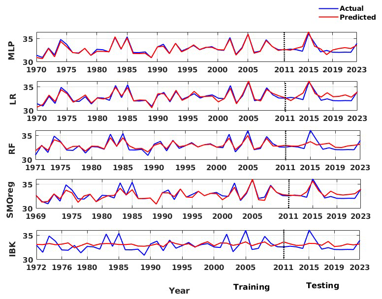
Figure 18 Actual vs. predicted values of log seismic energy from various individual techniques adopted for the Western Himalayan region.

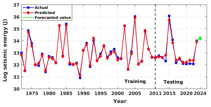
Figure 19 Actual vs. predicted values of seismic energy for the Western Himalayan region from the developed ensemble random forest model. The green marker shows the forecasted value for the year 2024.

7 Discussion

This work investigated the application of sophisticated machine learning (ML) algorithms for seismic energy predictions. The proposed work is significant in quantifying the immediate hazard for the region. It is well known that seismic energy is a potential indicator of seismic activity in the region. Thus, a reliable forecast through robust algorithms shall aid in the enhancement of hazard preparedness. The research systematically investigates this hypothesis by creating and comparing various machine learning models to identify their potential in seismic prediction. Therefore, an exhaustive modelling with five different architectures reflective of various machineries in machine learning is first attempted. The model approaches considered are the multi-layer perceptron (MLP), ridge regression (RR), random forest (RF), sequential minimal optimization for regression (SMOreg), and k-nearest neighbours (IBk). Examining the separate models, it was found that MLP consistently performed better than the others during the training and testing stages. The strong performance of MLP indicates that it might be a good fit for encapsulating intricate connections in seismic data. The model predictions from different architectures were observed to vary in the training and testing phases. Thus, the different ways in which these models function highlight how crucial it is to choose an algorithm that is suitable for the features of the seismic data. To improve the robustness of the prediction, the separate models (weak models) were combined to create an ensemble RF model. The outcomes showed that the ensemble model outperformed the single models, highlighting the possible advantages of mixing several modelling techniques. Furthermore, when comparing the ensemble model to the Raghukanth et al. (2017) model, the variance is lower, which suggests that the seismic energy forecasts are more stable and reliable. This research used train–test validation to ensure impartiality in model choice and to prevent overfitting through hyperparameter optimization using the training data. The method delivers an unbiased measure of generalization performance because it protects against any test exposure during model tuning. Our ensemble method is more consistent and has less error compared to the baseline model of Raghukanth et al. (2017) with the utilization of the same validation catalogue. This work contributes to the evidence for the model's robust generalization and excellent performance even in the absence of a third separate independent validation set. To further enhance resilience and evaluate learning frameworks under robust conditions, a separate validation dataset can be included in future work. Even though the study used a worldwide time series that covered the years 1900 to 2015, it is important to recognize any potential limitations related to this temporal scope. It is possible that patterns of seismic activity change and that some recent occurrences go unrecorded. In order to overcome this constraint and maintain the predictive accuracy and relevance of the results, future research should train models on an updated catalogue. Updated research (e.g. Sharma et al., 2023a; Kumar et al., 2023b) has established the advantage of using recent datasets in enhancing model generalizability. The study's encouraging findings provide opportunities for more investigation. Thus, as a sample study, a regional-level forecast model is developed for the Western Himalayan region. Similar to the global model, the regional data performance in forecasting improved while adopting an ensemble architecture. Even though the results are promising, the analysis is done on a larger cluster combining four seismogenic zones in the region. Such pooling, although streamlining model construction, can veil localized spatiotemporal features of prime importance to accurate hazard estimation. A more detailed physics-based clustering and further application to forecast modelling is expected to provide more insights into the spatiotemporal patterns of seismic activity. A more sophisticated knowledge of seismic energy trends may be obtained by extending the research to a more recent catalogue and carrying out extensive regional-level investigations on a regular basis. Furthermore, the present study acknowledges that ensemble empirical mode decomposition (EEMD) is adept at addressing non-stationarity in seismic energy time series; however, it also presents challenges, including edge effects, residual noise due to incomplete ensemble averaging, and constraints in accurately representing end-point behaviour. These limitations can affect the signal accuracy and can ultimately affect the performance of the seismic energy forecasts. Hence, in order to improve the forecasting capabilities and to address present limitations, future studies may explore more advanced time series decomposition techniques like wavelet-based denoising, complete ensemble EMD with adaptive noise (CEEMDAN), or hybrid filtering methods that enhance signal structure preservation and minimize noise interference. A further potential direction is uncertainty-conscious modelling, where the confidence interval of predictions is explicitly defined to enable risk-based decision-making. Furthermore, combining various seismogenic zones into larger clusters, although beneficial for this initial analysis, could potentially mask specific localized spatiotemporal seismic patterns. Therefore, upcoming models ought to integrate physics-informed regional clustering to improve the spatial resolution. From a machine learning perspective, the ensemble random forest model showed enhanced performance compared to individual models. Furthermore, the potential to improve the accuracy of the forecast model through a rigorous feature selection approach can also be adopted. These shall be taken as the future scope of this work. Additionally, there are intriguing prospects to improve forecasting accuracy further and capture complex patterns in seismic data by exploring more sophisticated and hybrid machine learning techniques like deep learning, the extreme learning machine (ELM), and generative adversarial networks (GANs). The use of explainable ML approaches (e.g. SHAP or LIME) will further improve model interpretability – a crucial step towards establishing trust in model outputs for stakeholders concerned with policy and hazard response. The advancements in time series preprocessing, spatial modelling, and predictive algorithms are anticipated to significantly improve the accuracy, robustness, and practical application of seismic energy forecasting models. This, in turn, will facilitate more effective early warning systems and strategies for hazard mitigation.

8 Conclusions

It has been found that using an appropriate ensemble model greatly increases the model's accuracy in predicting seismic energy, especially when handling the non-linearity and inherent complexity of geophysical data. The suggested method was then used to predict seismic energy for the Western Himalayas based on the assurance provided by testing with published data and a published methodology. The outcomes demonstrate the model's applicability in situations involving regional hazards. According to the proposed model, the total annual seismic energy in 2024 is expected to be between 9.11 × 10¹⁴ and 5.69 × 10¹⁴ J, or a magnitude range of 7.03–7.17. Therefore, we may anticipate that the Western Himalayan region would see a maximum magnitude of M_w 7.17. This study serves as a prototype project aimed at forecasting seismic energy release in the Himalayan region. With the appropriate adjustments, the framework developed here can be expanded or modified for use in other tectonically active areas. The future focus of this work will be on seismic energy patterns. However, the findings and recommendations of the study are essential for developing appropriate policy formulations, hazard preparedness, urgent risk assessment, and seismic resilience specific to a given location.