Climate change impacts on floods in West Africa: new insight from two large-scale hydrological models

West Africa is expected to face unprecedented shifts in temperature and extreme precipitation patterns as a result of climate change. The devastating impacts of river flooding are already being felt in most West African countries, emphasizing the urgent need for comprehensive insights into the frequency and magnitude of floods to guide the design of hydraulic infrastructure for effective flood risk mitigation and water resource management. Despite their significant socioeconomic and environmental impacts, flood hazards remain poorly documented in West Africa due to the data-related challenges. This study aims to fill this knowledge gap by providing a large-scale analysis of flood frequency and magnitudes across West Africa, focusing on how climate change may influence future flood trends. To achieve this, we have used two large-scale hydrological models driven by five bias-corrected sixth Coupled Model Intercomparison Project (CMIP6) climate models under two Shared Socioeconomic Pathways (SSPs). The generalized extreme value (GEV) distribution was utilized to analyze trends and detect change points by comparing multiple non-stationary GEV models across historical and future periods for a set of 58 catchments. Both hydrological models consistently projected increases in flood frequency and magnitude across West Africa despite their differences in hydrological process representations and calibration schemes. Flood magnitudes are projected to increase at 94 % (96 %) of stations for the 2-year (20-year) event in the near-term future and at 88 % (93 %) of stations for the 2-year (20-year) event in the long-term future, with some locations expected to experience increases exceeding 45 %. The findings from this study provide regional-scale insights into the evolving flood risks across West Africa and highlight the urgent need for climate-resilient strategies to safeguard populations and infrastructure against the increasing threat of flood hazards.

1 Introduction

Anthropogenic changes in atmospheric composition and land use have led to climate change (Houghton et al., 2001; Hansen et al., 2010; Santer et al., 2019; Masson-Delmotte et al., 2021). Climate change, in turn, amplifies the frequency, intensity, and impact of extreme events, such as heat waves, storms, floods, and droughts at the global scale (IPCC, 2021). West Africa is identified as a hotspot for climate change impacts, as the region is projected to experience unprecedented shifts in both temperature and extreme precipitation patterns (IPCC, 2021). West African populations are therefore becoming increasingly vulnerable to floods and droughts (Tramblay et al., 2020; Rameshwaran et al., 2021). This vulnerability is due to multiple factors such as the region's reliance on rainfed agriculture and the dependence of its rural communities on the natural environment (Krishnamurthy et al., 2012; Totin et al., 2016; Land et al., 2018; Diallo et al., 2020; De Longueville et al., 2020; Matthew et al., 2020). Additionally, the limited economic and institutional resources available to manage and adapt to climate change and natural hazards exacerbate this vulnerability (Roudier et al., 2011; Sultan and Gaetani, 2016; Lalou et al., 2019).

A potential increase in river flooding risks is one of the most frequently studied impacts of climate change (Arnell and Gosling, 2016) because of the devastating economic and environmental impacts it may trigger (EM-DAT, 2015; CRED, 2022; UNDRR, 2023). Such impacts of climate change are already being felt in many West African countries, which experienced several catastrophic floods in the past few years, raising concerns about water management and livelihoods (Lajaunie et al., 2021). It is therefore becoming crucial to develop efficient adaptation strategies to mitigate the adverse effects of flood hazards on West African communities and economies.

Efficient water resource management is essential for sustainable development in West Africa under a changing climate (UNEP, 2021). However, water management requires comprehensive insights into the frequency and magnitude of floods to design appropriate hydraulic infrastructure (Feaster et al., 2023) and quantification of watershed runoff to design reservoirs for agricultural, industrial, and municipal water use (Song et al., 2022). In West Africa, however, access to hydrometric data remains a challenge, as the number of stations within hydro-monitoring networks has decreased in recent years (Bodian et al., 2020; Tarpanelli et al., 2023). Existing hydrometric databases, available to estimate design flows, only provide short and often old records (Agoungbome et al., 2018; Tramblay et al., 2021). Therefore, updating these design flood estimation values (i.e., the ones used to build dams or reservoirs) is essential to ensure that they accurately represent the current hydroclimatic context of the region (Wasko et al., 2021)

Global climate model (GCM) outputs from the fifth/sixth Coupled Model Intercomparison Project (CMIP5/6), which contributed to the fifth and sixth Assessment Report (AR5/6) of the Intergovernmental Panel on Climate Change (IPCC), have provided opportunities to simulate future hydrological impacts of climate change worldwide. Indeed, CMIP5/6 models use a range of scenarios that represent different future trajectories to simulate several climate variables, which help researchers assess the potential long-term impacts of near-term decisions on emissions reductions and climate policies (Riahi et al., 2017). To understand future trends in hydrological extremes, climate models are typically used in combination with hydrological modeling experiments. However, the simulations from GCMs cannot be used to drive hydrological models directly as they are associated with systematic biases relative to observational datasets (Sillmann et al., 2013). Therefore, downscaling and bias-correction algorithms are routinely applied to leverage the information from GCM outputs (Ehret et al., 2012). Nevertheless, large uncertainties remain regarding future climate trends in West Africa, partly due to differences in how climate models simulate projected warming of the North Atlantic and Mediterranean Sea, affecting the West African monsoon and projected rainfall changes in the region (Bichet et al., 2020; IPCC, 2021; Monerie et al., 2023).

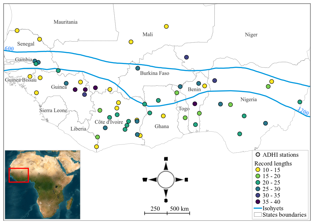
Figure 1 Spatial distribution of the stations used in this study, covering the three climatic zones in the West African region, as delimited by the blue isohyets (600 and 1200 mm annual rainfall) on the map. The color of the circles indicates the record lengths of flood data (in years). The gray lines indicate the borders of West African countries (African map from NASA 2005).

As climate change may intensify the hydrological cycle (Gudmundsson et al., 2012), systematically assessing future flood risks and the regional-scale hydrological impacts of future climate change is crucial to develop effective climate adaptation strategies (Huang et al., 2024). Due to their simplicity and computational efficiency, lumped hydrological models have been widely applied in West Africa (Niel et al., 2003; Bodian et al., 2016, 2018; Kwakye and Bárdossy, 2020; Koubodana et al., 2021). However, because runoff generation is an inherently spatial and temporally dynamic process, changing environmental conditions may impact flood frequencies and water availability (Wilson et al., 1979; Haddeland et al., 2002; Descroix et al., 2018). Although lumped models often perform comparably or even better than distributed models at the catchment outlet (Reed et al., 2004), their main limitation lies in evaluating the overall catchment response at the outlet alone without accounting for the contributions of individual sub-basins upstream (Pokhrel et al., 2008; Jajarmizad et al., 2012). The main advantage of distributed models is not necessarily a higher accuracy of runoff simulations at specific points (e.g., outlet or gauge stations) but rather their broader applicability and the ability to simulate the impacts of spatially varying drivers and scenarios (Gebremeskel et al., 2005; Tang et al., 2007; Thielen et al., 2009; Chu et al., 2010; Tran et al., 2018). The interest in large-scale hydrological models has increased due to the need to sustainably manage large river basins and because of the pervasive global environmental change. As global hydrological models can capture the variability in hydrological processes across different geographical and climatic contexts, large-scale hydrological modeling has become a key tool for analyzing global and regional water resources, assessing climate impacts, and managing water resources (Kauffeldt et al., 2013; Prudhomme et al., 2024). However, running physically based large-scale hydrological models requires numerous input variables that describe the physiographic characteristics of the watersheds (soil moisture, land use/land cover, topography, etc.), along with several meteorological forcings. Thus, this complexity limits the widespread use of these models. Brunner et al. (2021) have argued that the limited information on regional flood trends is partly due to the data-related challenges. In the West African context, several studies have shown the increase in extreme rainfall in observations (Taylor et al., 2017; Tramblay et al., 2020; Chagnaud et al., 2022) and in future climate scenarios (Dosio et al., 2021; Chagnaud et al., 2023), but very few studies have used GCM simulations as forcings to drive grid-based large-scale hydrological models to assess the potential impacts of climate change on river flows across West Africa (Rameshwaran et al., 2021; Ekolu et al., 2024, https://africa-hydrology.ceh.ac.uk/, last access: 4 September 2025). The main objective of this study is to address this gap by assessing the impacts of climate change on floods in the West African region from two large-scale hydrological models driven by data from five bias-corrected CMIP6 GCMs under two Shared Socioeconomic Pathways (SSPs; O'Neill et al., 2017). This article is organized as follows: Section 2 outlines the materials and methods, including the data used in the analysis, the CMIP6 models and hydrological modeling approach, the non-stationary extreme value analysis framework, and the evaluation of climate change impacts on floods at both local and regional scales. In Sect. 3, we present and discuss the findings. Finally, the main conclusions and perspectives are given in Sect. 4.

2 Materials and methods

2.1 Study area description

West Africa covers about one-fifth of the African continent, extending from the Atlantic coast of Senegal (18° W) to eastern Chad (25° E) and from the Gulf of Guinea (4° N) to the Sahel (25° N) (Fig. 1). The region's climate is governed by the Inter-Tropical Convergence Zone (ITCZ) or the Inter-Tropical Discontinuity (ITD), which represent the interface at the ground between moist monsoon air and dry harmattan air with a migratory annual cycle (Pospichal et al., 2010). The West African region features high climatic diversity (Vintrou, 2012) and covers a wide range of ecosystems and bioclimatic regions (Nicholson, 2018). The latitudinal and seasonal oscillation of the ITCZ divides the region into three main climatic domains, namely the Sahel, Sudanian, and Guinean zones (Sule and Odekunle, 2016). The Sahel zone is a semi-arid region with a short rainy season and an annual average rainfall not exceeding 600 mm (Fig. 1). This domain is highly vulnerable to the adverse effects of climate change (Tian et al., 2023). The Sudanian zone stretches as a broad belt south of the Sahel, receiving an average rainfall of 600 to 1200 mm. The Guinean zone, known for its rugged terrain with steep slopes (Orange, 1990), receives abundant rainfall throughout the year, with an annual average between 1200 and 2200 mm. These three climate zones are characterized by distinct vegetation (Biaou et al., 2023) and rainy-season patterns. The Sahelian and Sudanian domains share a unimodal rainfall pattern, while the Guinean zone experiences a bimodal rainfall pattern of two rainy seasons driven by the West African monsoon (Rodríguez-Fonseca et al., 2015; Nicholson, 2018). It is worth noting that nearly half of African watersheds are located in West Africa. The socioeconomic development (agriculture, energy production, and livelihoods) of the region relies highly on the water resources provided by these transboundary basins and aquifers.

2.2 Observational data and climate forcings for hydrological experiments

Daily streamflow data for the period of 1950–2018 were obtained from the African Database of Hydrometric Indices (ADHI) recently developed by Tramblay et al. (2021) and used for a local flood frequency study in West Africa by Diop et al. (2025). This database provides hydrometric indices computed from different data sources, with daily discharge time series that span at least 10 years. In the ADHI database, the size of the 441 West African catchments ranges from 95 to 2 150 000 km², and some stations have daily discharge data spanning 44 years. Figure 1 shows the spatial distribution of the ADHI stations used in this study, and Table S1 in the Supplement gives information on their geographical locations (longitude and latitude), catchment areas, mean annual catchment-averaged rainfall, mean annual streamflow, and the range of years over which streamflow data are available. We only selected watersheds from the ADHI database that met the following three criteria: (i) low regulation, determined through visual inspection of dam locations relative to watershed outlets (see Fig. S1 in the Supplement), combined with a year-by-year analysis of annual hydrographs to assess the impact of dam operations on streamflow; (ii) surface area of less than 150 000 km²; and (iii) a daily streamflow time series covering a minimum of 10 years between 1950 and 2018. To address the challenges associated with missing data in the database, we conducted a visual inspection of hydrographs at each station, as illustrated by Fig. S2 in the Supplement. Years with data gaps near the flood peak were excluded from the analysis to avoid the risk of missing the true annual peak flood (Wilcox et al., 2018). Through this careful screening process, we ensured that no annual maximum flow (AMF) values were derived from periods characterized by a lot of missing data. It is important to note that the observational streamflow data are not used to calibrate or drive the hydrological models. Instead, these observations serve as an independent benchmark to evaluate the ability of the hydrological models to reproduce key flood statistics during the historical period. The LISFLOOD model was calibrated using the ERA5 reanalysis dataset, which provides consistent and high-resolution precipitation and temperature fields. Moreover, ERA5 was also used as a reference for the bias correction of the five climate models from the CMIP6 ensemble that were used to drive the hydrological simulations for both the historical and future periods (see Sect. 2.4).

2.3 Hydrological models

Two grid-based large-scale hydrological models were used to simulate river flows for the period from 1950 to 2010: the HMF-WA model (the Hydrological Modeling Framework for West Africa; Rameshwaran et al., 2021) and the open-source (OS) LISFLOOD model (Van Der Knijff et al., 2010), hereafter referred to as LISFLOOD. The HMF-WA model is adapted from the modular HMF model and is designed for large-scale applications across West Africa (Rameshwaran et al., 2021). It employs a vertically integrated soil moisture scheme to simulate runoff production driven by rainfall and potential-evaporation inputs. Runoff generation considers soil drainage and a spatial probability distribution of soil moisture. Routing is based on a kinematic wave approach (Bell et al., 2007), with parallel pathways for surface and subsurface flow. Key enhancements over the classical HMF model include modules to simulate wetland inundation, endorheic basins, and anthropogenic water withdrawals, making it well-suited for semi-arid environments with complex hydrology (Rameshwaran et al., 2021). HMF-WA simulates spatially consistent river flows across West Africa at a 0.1° × 0.1° spatial resolution. Although it has not yet been specifically calibrated to individual West African catchments using observed streamflow data where the model hydrology is configured to local conditions using spatial datasets of physical and soil properties, HMF-WA model evaluation against observational data indicates that it performs reasonably well when simulating both daily high and low river flows across most catchments. The median values of NSE (Nash–Sutcliffe efficiency), NSElog, and relative bias are 0.62, 0.82, and 0.06 (6 %), respectively (Rameshwaran et al., 2021).

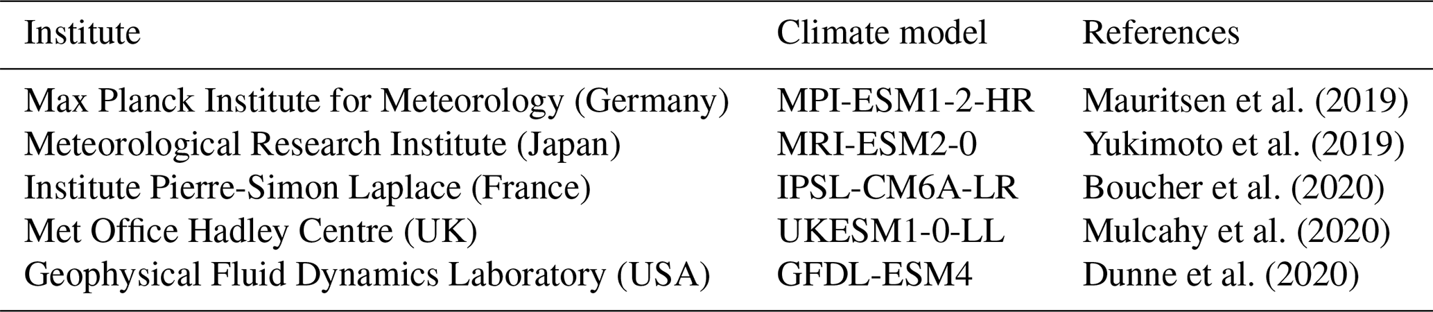
Table 1 The bias-corrected CMIP6 climate models used in this study.

The LISFLOOD model, developed by the Joint Research Centre (JRC) of the European Commission (https://ec-jrc.github.io/lisflood/, last access: 4 September 2025), is a physical spatially distributed hydrological model designed to simulate several hydrological processes that occur in a catchment (Van Der Knijff et al., 2010). The LISFLOOD model simulates water processes using a three-layer soil water balance, along with groundwater and subsurface flow models. It accounts for several processes such as snow accumulation/melt, infiltration, evapotranspiration, groundwater flow, and surface runoff. Moreover, it supports the integration of human influences such as reservoirs and water abstraction. The numerical LISFLOOD simulation is driven by meteorological forcing (precipitation, temperature, and evapotranspiration) combined with high-resolution spatial data on terrain morphology, soil characteristics, land use, and water demand. This integrated setup allows the model to simulate runoff processes under diverse climatic and socioeconomic conditions, capturing both natural and anthropogenic influences across heterogeneous landscapes. The runoff produced at every grid cell within the model domain is routed through the river network using a kinematic wave approach. The LISFLOOD version used in this study (OS LISFLOOD v4.1.3) was calibrated with a 0.05° (∼ 5 km) resolution in its quasi-global implementation, covering a longitude range from 180° W to 180° E and a latitude range from 90° N to 60° S, using in situ discharge gauge stations with at least 4 years of daily measurements recorded after 1 January 1982. In this setup, model parameters are linked to global geospatial datasets describing catchment morphology and river networks, land use, vegetation characteristics, soil properties, lake distribution, and water demand (Salamon et al., 2023; Choulga et al., 2024). The distributed evolutionary algorithms in Python (DEAP; Fortin et al., 2012) framework was applied to optimize parameters in gauged catchments, with the modified Kling–Gupta efficiency (KGE; Gupta et al., 2009) utilized as the objective function. Calibration was performed over a continuous simulation period using ERA5 reanalysis meteorological forcing. Due to the varying length and temporal coverage of the discharge records used for calibration, model performance was assessed using all available observational data at each station rather than splitting the records into separate calibration and validation periods. The LISFLOOD calibration tool is freely available at https://github.com/ec-jrc/lisflood-calibration (last access: 4 September 2025).

Globally, while both models use a kinematic wave routing scheme, HMF-WA and LISFLOOD differ significantly in their hydrological process representation. HMF-WA applies a vertically integrated soil moisture scheme with simplified runoff generation based on spatial soil moisture distributions. In contrast, LISFLOOD features a more detailed physically based three-layer soil model with an explicit representation of groundwater, snow processes, and anthropogenic influences. Furthermore, LISFLOOD has been calibrated using in situ discharge data. Nevertheless, while calibration can enhance the accuracy of discharge simulations, several studies have highlighted the fact that uncalibrated global hydrological models often exhibit similar sensitivity to climate variability compared to the region-calibrated hydrological models, particularly when assessing relative changes in extreme events between future and historical periods (Gosling et al., 2017; Zhao et al., 2025). Therefore, whether a calibrated hydrological model offers different climate change projections compared to an uncalibrated model needs further investigation (Pechlivanidis et al., 2017).

2.4 Bias-corrected CMIP6 models and scenarios

The sixth phase of the Coupled Model Intercomparison Project (CMIP6) provides simulations from GCMs for the preindustrial period (1850–2014) and future climate projections (2015–2100) (Noël et al., 2022). To assess future climate impacts on floods, we have used five daily GCM rainfall and temperature outputs from the CMIP6 experiments (https://esgf-node.llnl.gov/search/cmip6, last access: 4 September 2025). Table 1 gives the institute name and references of the CMIP6 climate models used in this study. These GCMs encompass a range of climate sensitivities, with equilibrium climate sensitivity (ECS) values ranging from 2.98 to 5.34 (IPCC, 2021). The GCMs were selected based on their availability for the study area. Due to their accessibility, these GCMs have been widely used for climate impact assessments in Africa (Dosio et al., 2019; Almazroui et al., 2020; Klutse et al., 2021; Babaousmail et al., 2023; Nooni et al., 2023). The cumulative distribution function – transform (CDF-t) (Michelangeli et al., 2009) was used to bias-correct the GCM outputs. The CDF-t approach involves mapping the cumulative distribution function (CDF) from a GCM in the historical period to the observed CDF, then applying the same mapping to the GCM's future CDF (Flaounas et al., 2013; Famien et al., 2018). The CDF-t method requires high-resolution observational data to work properly. The EWEMBI dataset (E2OBS, WFDEI, and ERA-I data bias-corrected for ISIMIP; Frieler et al., 2017; Lange, 2018, 2019) was used to bias correct the climate variables to drive the HMF-WA hydrological model. Similarly, the ERA5-land reanalysis (Muñoz-Sabater et al., 2021) was used to bias correct the GCM outputs for the LISFLOOD model. The EWEMBI dataset was developed to support bias correction of the climate input data used in impact assessments in phase 2b of the Inter-Sectoral Impact Model Intercomparison Project (ISIMIP2b; Frieler et al., 2017). The EWEMBI dataset (https://dataservices.gfz-potsdam.de/pik/showshort.php?id=escidoc:3928916, last access: 4 September 2025) provides global spatial coverage with 0.5° × 0.5° spatial and daily temporal resolutions. It integrates multiple sources, including ERA-Interim reanalysis data (Dee et al., 2011), the WATCH Forcing Data methodology applied to ERA-Interim (WFDEI; Weedon et al., 2014), the eartH2Observe forcing dataset (E2OBS; Calton et al., 2016), and the NASA/GEWEX Surface Radiation Budget data (SRB; Stackhouse et al., 2011). Meanwhile, the ERA5 dataset is a global atmospheric reanalysis product developed by the Copernicus Climate Change Service (C3S) at ECMWF (European Centre for Medium-Range Weather Forecasts ReAnalysis). It is the fifth generation of atmospheric reanalysis based on 4D-Var (four-dimensional variational) data assimilation using Cycle 41r2 of the ECMWF Integrated Forecasting System (IFS) (Hersbach et al., 2020). ERA5 replaces the now outdated ERA-Interim reanalysis (Dee et al., 2011) and provides global spatial coverage from 1979 until the present, with a finer spatial and temporal resolution of 0.25° × 0.25° and 1 h, respectively. The bias-corrected simulations are post-processed onto the 0.1° × 0.1° (∼ 10 km × 10 km) HMF-WA model grid (Rameshwaran et al., 2021, 2022) and onto the 0.05° × 0.05° (∼ 5 km × 5 km) LISFLOOD model grid for the period of 1950–2100. CMIP6 models use five Shared Socioeconomic Pathways (SSPs). SSPs are an updated framework of climate scenarios, building upon the CMIP5 Representative Concentration Pathways (RCPs) while maintaining consistency with the 2100 radiative forcing levels. SSPs describe the socioeconomic factors (population growth, economic development, technological advancements, and governance) that can influence greenhouse gas emissions and adaptation strategies (O'Neill et al., 2017). Two Shared Socioeconomic Pathways (SSPs) are analyzed in this study: the SSP2-4.5 (middle of the road) and the SSP5-8.5 (fossil-fueled development). Rather than including the full range of SSPs, we focus on the SSP2-4.5 and SSP5-8.5 narratives, which represent moderate- and high-emission trajectories, respectively. SSP2-4.5 is considered a middle-of-the-road scenario that is consistent with current national policies and moderate progress towards emission reduction commitments. In contrast, SSP5-8.5 represents a high-emissions pathway, allowing us to explore the upper limits of potential impacts under continued fossil fuel dependence and minimal climate policy intervention. While SSP5-8.5 has been criticized as an “overly pessimistic” narrative (Pielke and Ritchie, 2021), it remains widely used in climate impact assessments to evaluate the vulnerability of socio-environmental systems under a “no-climate-policy” world.

2.5 Evaluation of hydrological models

The two hydrological models are evaluated over the period of 1950–2014, which represents a compromise between the period covered by the ADHI database and the historical CMIP6 GCM simulations. To achieve this, we use the two-sample Anderson–Darling (AD) test at the 0.05 significance level (Scholz and Stephens, 1986) to compare the distributions of extreme values observed and simulated by the hydrological models. The null hypothesis of the AD test assumes that the simulated and observed AMF follow the same statistical distribution. The block-maxima approach (Gumbel, 1958) is used to construct extreme value time series by extracting the annual maximum flow (AMF) from the daily discharge time series over the period of 1950–2014. Unlike the Kolmogorov–Smirnov (KS) test (Berger and Zhou, 2014), which measures the maximum distance between two cumulative distribution functions (CDFs), the AD test assesses the overall distance between these CDFs, giving more weight to the tails of the distributions. As a result, the AD test is more sensitive than the KS test in the tails of distributions and is therefore more suitable for comparing extreme-value distributions (Engmann and Cousineau, 2011). That said, the AD test also has a limitation, as the reliability of an empirical CDF can be affected by small sample sizes, particularly in the tails of the distribution. The performance of each hydrological model is given here by the proportion of CMIP6 simulations (among the five) for which the AD test has failed. It is important to note that the AD test is only used herein to assess regional-scale performance of hydrological models and is not used as a filtering criterion for inclusion or exclusion of models or stations.

2.6 Extremes value analysis framework

2.6.1 The generalized extreme value distribution

According to the theory of extreme values based on the Fisher–Tippett theorem, the generalized extreme value (GEV) is the limiting distribution of independent and identically distributed random variables (Coles, 2001). The GEV is among the most frequently used distributions for extreme value analysis. It is a continuous three-parameter distribution that can account for non-stationarity, which refers to changes in statistical properties over time. This is achieved by allowing the parameters to vary as a function of time or other covariates (Hamdi et al., 2018; Wilcox et al., 2018). We, therefore, used the GEV to model the AMF series from each hydrological model simulation forced with the five CMIP6 climate models at each catchment. There are three parameters (location, scale, and shape) in the GEV distribution (Hossain et al., 2021). In flood frequency analysis, each GEV parameter plays a distinct role in understanding and projecting flood behavior (Lawrence, 2020; Wasko et al., 2021). The location parameter (μ) indicates the central tendency of flood magnitudes, with higher values suggesting a shift towards more frequent or severe floods. The scale parameter (σ) measures the variability or dispersion of the distribution, with larger values indicating greater uncertainty and a broader range of flood magnitudes. The shape parameter (ξ) governs the tail behavior of the GEV distribution, which encompasses three types of extreme value distributions (Coles, 2001): (i) a positive shape parameter (ξ >0) indicates a heavy-tailed Fréchet case (Fréchet, 1927), suggesting an increased probability of extreme flooding events; (ii) a null shape parameter (ξ = 0) suggests a light-tailed Gumbel class (Gumbel, 1958); and (iii) a negative shape parameter (ξ <0) indicates a short-tailed or (bounded) negative-Weibull distribution (Weibull, 1951). This parameter is crucial to assess the risk of rare floods and to inform the choice of design infrastructure to withstand such extremes. Equation (1) presents the cumulative distribution function (CDF) of the GEV (Coles, 2001).

$$\begin{array}{}\text{(1)}& \begin{array}{rl}& F(x;u,\mathit{\alpha },\mathit{\xi })=\exp \left\{-{\left[\mathrm{1}-\mathit{\xi }{\displaystyle \frac{(x-u)}{\mathit{\alpha }}}\right]}^{\mathrm{1}/\mathit{\xi }}\right\}\mathit{\kappa }\ne \mathrm{0}\\ & F(x;\mathit{\xi },\mathit{\alpha })=\exp \left\{-\exp \left[-{\displaystyle \frac{(x-u)}{\mathit{\alpha }}}\right]\right\}\mathit{\kappa }=\mathrm{0}\end{array}\end{array}$$

x, u, α, and ξ are the data, location, scale, and shape parameters, respectively, and $(u+\mathit{\alpha }/\mathit{\xi })\le x<\mathrm{\infty }$ if ξ<0; $-\mathrm{\infty }<x<\mathrm{\infty }$ if ξ=0; $-\mathrm{\infty }<x\le (u+\mathit{\alpha }/\mathit{\xi })$ if κ>0.

Efficiently estimating the GEV parameters is crucial for the precise characterization and analysis of extreme events (Rai et al., 2024). We have used the generalized (penalized) maximum likelihood estimation (GMLE) method (Martins and Stedinger, 2000) to estimate the GEV parameters in a non-stationary context by allowing the model parameters to vary with time (Coles, 2001). The GMLE method overcomes the limitations of the well-known maximum likelihood estimation (MLE; Fisher, 1992) method for small sample sizes (Hossain et al., 2021). To achieve this, Martins and Stedinger (2000) used a beta distribution (with shape parameters p = 6 and q = 9) as a prior to constrain the values of the GEV shape parameter in the interval [$-\mathrm{0.5},+\mathrm{0.5}$], avoiding large negative values of the shape parameter. This approach has been used in several studies to estimate the GEV parameters in both stationary and non-stationary contexts (El Adlouni et al., 2007; Panthou et al., 2013; Tramblay et al., 2024). However, the original prior distribution from Martins and Stedinger (2000) is not well-suited to West Africa, as it results in shape parameter estimates below −0.5 for several stations, as illustrated in Fig. S3 in the Supplement. Here, we therefore use a normal distribution as a prior for the GMLE method. This normal distribution is fitted to the GEV shape parameter values estimated from 98 AMF series spanning a minimum of 20 years over the period of 1950–2018 from the ADHI database (Tramblay et al., 2021) using the L-moments method (Hosking, 1990). The newly developed regional prior, modeled as a normal distribution, has a mean of −0.24 and a standard deviation of 0.16 (see Fig. S3) and is used to fit the GEV distribution to the historical and projected annual peak flood time series generated by the hydrological models driven by the CMIP6 GCMs.

2.6.2 Determining the magnitude and direction of changes in flood events

To analyze future changes in floods, we compare two 30-year future periods (a near-term future (2031–2060) and a long-term future (2071–2100)) to a reference historical period (1985–2014) at stations where there is a good fit between observed (OBS) AMF series and hydrological model simulations (HIST) according to the Anderson–Darling (AD) test (at 0.05 level) and also at stations at which the null hypothesis of the AD test is rejected. We have chosen to work with the 2- and 20-year floods to analyze the impacts of climate change in West Africa. The 2-year return period indicates relatively frequent flood events, and this information is essential to understand and manage the risks associated with flooding. The 20-year flood event is frequently used for comparative purposes in various studies, as it balances the rarity of extreme events (data length limitations) and the uncertainty in the estimated return levels (Dawson et al., 2005; Tramblay and Somot, 2018; Han et al., 2022). Thus, the 2- and 20-year flood quantiles are computed at each station for the three 30-year periods, using the GEV model fitted to the AMF series by the GMLE method. Changes in floods are quantified in this study by computing the ratio of the difference between the future flood quantile (Qfuture) and the historical flood quantile (Qhist) to Qhist itself. To assess the statistical significance of the differences between the historical and future flood quantiles, we have used the parametric bootstrapping approach. After estimating the GEV distribution parameters, we have generated 2500 simulations of annual peak floods for each sub-period (with each simulation representing a sample of 30 data points). We have then recomputed the 2- and 20-year flood quantiles for each simulation. The significance of the differences between the quantiles was evaluated at the 0.05 level. It is crucial to consider the degree of consensus among multiple climate models to reduce the potential noise in the projections and to reach robust conclusions (Awotwi et al., 2021; Dosio et al., 2021). Here, we have computed a multi-model index of agreement (MIA) as introduced by Tramblay and Somot (2018) to present the results in terms of the proportion of CMIP6 models projecting significant change for each station. The MIA allows the assessment of the robustness of climate model projections, ensuring cross-catchment comparability due to its standardized scale ranging from −1 to 1 according to the direction of change (i.e., MIA = 1 (−1) if all models project an increasing (decreasing) trend).

$$\begin{array}{}\text{(2)}& \text{MIA}={\displaystyle \frac{\mathrm{1}}{n}}\left({\sum }_{m=\mathrm{1}}^n{i}_m\right)\end{array}$$

From Eq. (6), for a given CMIP6 model $\left(m\right),i_m=\mathrm{1}$ for regionally significant upward trends, $i_m=-\mathrm{1}$ for significant negative trends, and i_m=0 when no significant trends are detected across n climate simulations.

2.6.3 Determining temporal functions for GEV parameters and modeling of non-stationary extreme values

While the previous section focused on the magnitude and direction of changes in flood events under different scenarios, this section describes the methodology used to identify when these changes began. Understanding how the parameters of the GEV distribution might shift under future climate scenarios is a critical question that needs to be addressed given the accelerating impacts of global warming on environmental conditions. Answering this question can inform a more reliable modeling process to estimate flood quantiles. Several studies have suggested that both the location and scale parameters of the GEV distribution should be adjusted proportionally to account for the effects of climate change (Stedinger and Griffis, 2011; Prosdocimi and Kjeldsen, 2021; Jayaweera et al., 2024). Here, to determine the appropriate temporal function for the non-stationary GEV, the trends in GEV parameters are detected using the non-parametric Mann–Kendall test (Mann, 1945; Kendall, 1975). As the test is applied to parameters estimated over moving windows, it is important to note that temporal correlation is introduced, which can bias the results of the original Mann–Kendall test, as it assumes the independence of observations. To address this, we have applied a modified version of the test based on the Hamed and Rao (1998) variance correction approach, which is specifically adapted for serially correlated data. A window size of 30 years has been selected to ensure sufficient data to fit the stationary GEV model (SGEV), with a total of 121 windows. For each window, each hydrological model (LISFLOOD and HMF-WA), and each climate scenario (SSP2-4.5 and SSP5.8-5), the SGEV is fitted to AMF series from the averaged hydrological simulations driven by data from the CMIP6 models. The Mann–Kendall test is then applied to the series of estimated parameters at the 0.05 significance level.

Based on the results of the trend analysis of the GEV parameters, the location (μ) and scale (σ) parameters are expressed as linear functions of time, denoted μ(t) and σ(t), while the shape parameter remains constant. Thus, the non-stationary GEV model involves a vector $\mathit{\psi }=[\mathit{\mu }\mathrm{0};\mathit{\mu }\mathrm{1};\mathit{\sigma }\mathrm{0};\mathit{\sigma }\mathrm{1};\mathit{\xi }]$ of five unknown parameters. We have decided to keep the shape parameters constant because it is uncommon for researchers to model all three GEV parameters as covariate-dependent functions. Indeed, adding this level of complexity can significantly complicate the model parameter estimation, particularly the shape parameter (Katz, 2013; Papalexiou and Koutsoyiannis, 2013). Allowing any starting date (year t₀) for a possible significant trend in the GEV location and scale parameters, we have considered three cases of the non-stationary GEV (NSGEV; see Eqs. 3–5).

• Case 1 (GEV1). A linear trend with no breakpoint (i.e., a single trend over the entire record for both the location and scale parameters):

  $$\begin{array}{}\text{(3)}& \mathit{\mu }\left(t\right)={\mathit{\mu }}_{\mathrm{0}}+{\mathit{\mu }}_{\mathrm{1}}t;\mathit{\sigma }\left(t\right)={\mathit{\sigma }}_{\mathrm{0}}+{\mathit{\sigma }}_{\mathrm{1}}t\text{ for }t\le t_{\mathrm{0}}.\end{array}$$

• Case 2 (GEV2). A linear trend after a breakpoint (i.e., the location and scale parameters are constant before the year t₀ and are linearly dependent on time after t₀):

  $$\begin{array}{}\text{(4)}& \begin{array}{rl}& \mathit{\mu }\left(t\right)={\mathit{\mu }}_{\mathrm{0}};\mathit{\sigma }\left(t\right)={\mathit{\sigma }}_{\mathrm{0}}\text{ for }t\le t_{\mathrm{0}}\\ & \mathit{\mu }\left(t\right)={\mathit{\mu }}_{\mathrm{0}}+{\mathit{\mu }}_{\mathrm{1}}(t-t_{\mathrm{0}});\mathit{\sigma }\left(t\right)={\mathit{\sigma }}_{\mathrm{0}}+{\mathit{\sigma }}_{\mathrm{1}}(t-t_{\mathrm{0}})\text{ for }t\ge t_{\mathrm{0}}.\end{array}\end{array}$$

• Case 3 (GEV3). Both trends before and after a breakpoint are considered (i.e., a linear trend before and after year t₀ for both location and scale parameters):

  $$\begin{array}{}\text{(5)}& \begin{array}{rl}& \mathit{\mu }\left(t\right)={\mathit{\mu }}_{\mathrm{0}}+{\mathit{\mu }}_{\mathrm{1}}(t_{\mathrm{0}}-t);\mathit{\sigma }\left(t\right)={\mathit{\sigma }}_{\mathrm{0}}+{\mathit{\sigma }}_{\mathrm{1}}(t_{\mathrm{0}}-t)\text{ for }t\le t_{\mathrm{0}}\\ & \mathit{\mu }\left(t\right)={\mathit{\mu }}_{\mathrm{0}}+{\mathit{\mu }}_{\mathrm{1}}(t-t_{\mathrm{0}});\mathit{\sigma }\left(t\right)={\mathit{\sigma }}_{\mathrm{0}}+{\mathit{\sigma }}_{\mathrm{1}}(t-t_{\mathrm{0}})\text{ for }t\ge t_{\mathrm{0}}.\end{array}\end{array}$$

Unlike in Wilcox et al. (2018), where breakpoints are defined independently for μ(t) and σ(t), in the present study, we assume a common breakpoint for both parameters. This means that both μ(t) and σ(t) change simultaneously at the same point in time. To ensure that the NSGEV model is fitted with sufficient data, the first start year is set no earlier than 20 years after the beginning of the time series (1950), and the last start year is set no later than 20 years before the end of the time series (2100). Thus, the possible starting years of change (t₀) fall between 1970 and 2070. There are as many NSGEV models as there are breakpoints or starting years, and the non-stationary model with the highest log-likelihood is selected (see Fig. S4 in the Supplement). The procedure described above is inspired by several studies that focused on detecting trends in hydroclimatic time series using non-stationary GEV (Hawkins and Sutton, 2012; Panthou et al., 2013; Blanchet et al., 2018; Hamdi et al., 2018; Tramblay and Somot, 2018; Wilcox et al., 2018).

Once the best breakpoint has been determined for each time-varying GEV model based on the log-likelihood profile, the trend models (GEV1, GEV2, and GEV3) are compared with each other using the Akaike information criterion (AIC; Akaike, 1974). The AIC criterion is widely used to compare multiple statistical models by assessing their goodness-of-fit. It accounts for the trade-off between a model's fit to the data and its complexity by penalizing more complex models. While a more complex model may provide a better fit, it often does not provide sufficient improvement to justify the addition of extra parameters (Wilcox et al., 2018). Thus, the AIC is well-suited to evaluate the performance of non-stationary GEV models. Furthermore, a deviance test (D) based on the likelihood ratio (LR; Coles, 2001) is performed at the 0.05 significance level between the best GEV trend model selected previously based on the AIC criterion and the stationary GEV model (SGEV). The LR test allows us to determine the best model between two competing nested models by comparing the D statistic given by Eq. (6) to the chi-squared (χ²) distribution.

$$\begin{array}{}\text{(6)}& D=\mathrm{2}\mathit{\left\{}\text{log}\right({\text{ML}}_{\text{NSGEV}})-\text{log}({\text{ML}}_{\text{SGEV}}\left)\mathit{\right\}}\end{array}$$

From Eq. (6), D represents the deviance test statistic value (referred to as the D statistic above) and log(ML_NSGEV) and log(ML_SGEV) are the maximized log-likelihood functions of the NSGEV and the SGEV, respectively. Letting c_α be the (1 – α) quantile of the chi-squared distribution (where α represents the level of significance), with υ degrees of freedom equal to the difference in the number of model parameters between the non-stationary and stationary models, the non-stationary GEV is accepted at the level α if the D statistic is greater than c_α, meaning a significant trend in the data.

The null hypothesis of the deviance test assumes that the stationary GEV model provides a better fit to the data than the non-stationary model, indicating that there is no significant trend in the AMF. However, the presence of spatial cross-correlations across stations may bias the results of simultaneous multiple local tests by increasing the likelihood of detecting false positives (Farris et al., 2021). To assess the field significance of local trends detected in AMF series in the study area, we implement the false-discovery-rate (FDR) procedure (Hochberg and Benjamini, 1995). The FDR's null hypothesis assumes that none of the stations across the region exhibits a significant trend in AMF (i.e., all local null hypotheses are actually true). The FDR aims to reduce type-1 errors (Mudge et al., 2012) by adjusting the vector of p values from the set of at-site tests (Wilks, 2006). Due to its advantages over other methods, such as dealing with spatial autocorrelation, the FDR approach has been used in many studies of hydroclimatic variables (Khaliq et al., 2009). For consistency with local deviance and M–K tests, the FDR procedure is computed at the 0.05 global significance level (α global). The FDR test rejects the local null hypothesis when the corresponding FDR-adjusted p value is lower than α global. Field significance is declared if the local null hypothesis is rejected at least once within the study area (Wilks, 2016).

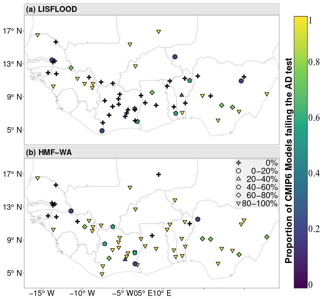
Figure 2 Statistical evaluation of the two hydrological models. (a) The two-sample Anderson–Darling (AD) goodness-of-fit (GOF) test at a 0.05 statistical significance level at each station between the AMF of daily OBS from the ADHI database and annual maxima flow of HIST from LISFLOOD daily simulations forced with the five CMIP6 GCMs (GFDL, IPSL, MPI, MRI, and UKESM) over the period of 1950–2014. (b) Same as (a) but using HMF-WA as the hydrological model. The fill color of the markers indicates the proportion of CMIP6 models (out of five) for which the AD test null hypothesis (i.e., simulated and observed AMF follow the same statistical distribution) is rejected at the 0.05 significance level. Marker shapes correspond to binned categories of this proportion, as indicated in the legend.

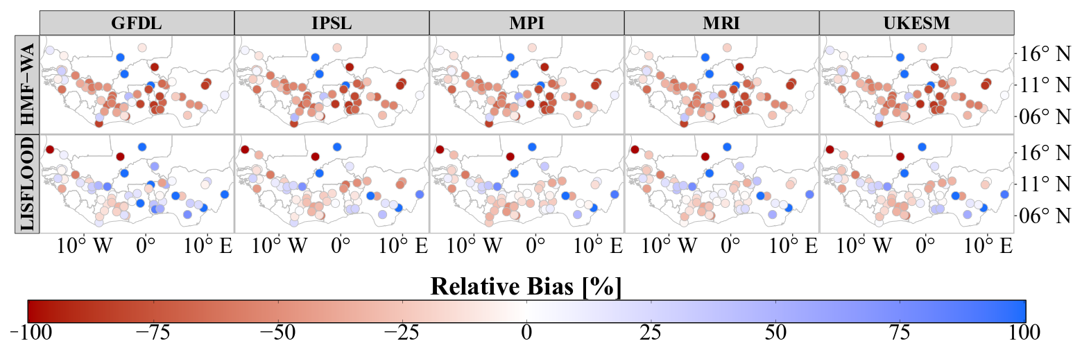
Figure 3 Relative bias (percentages) computed between simulated AMF from LISFLOOD-CMIP6 and HMFWA-CMIP6 hydrological models' simulations and observed AMF from the ADHI database for the historical period (1950–2014).

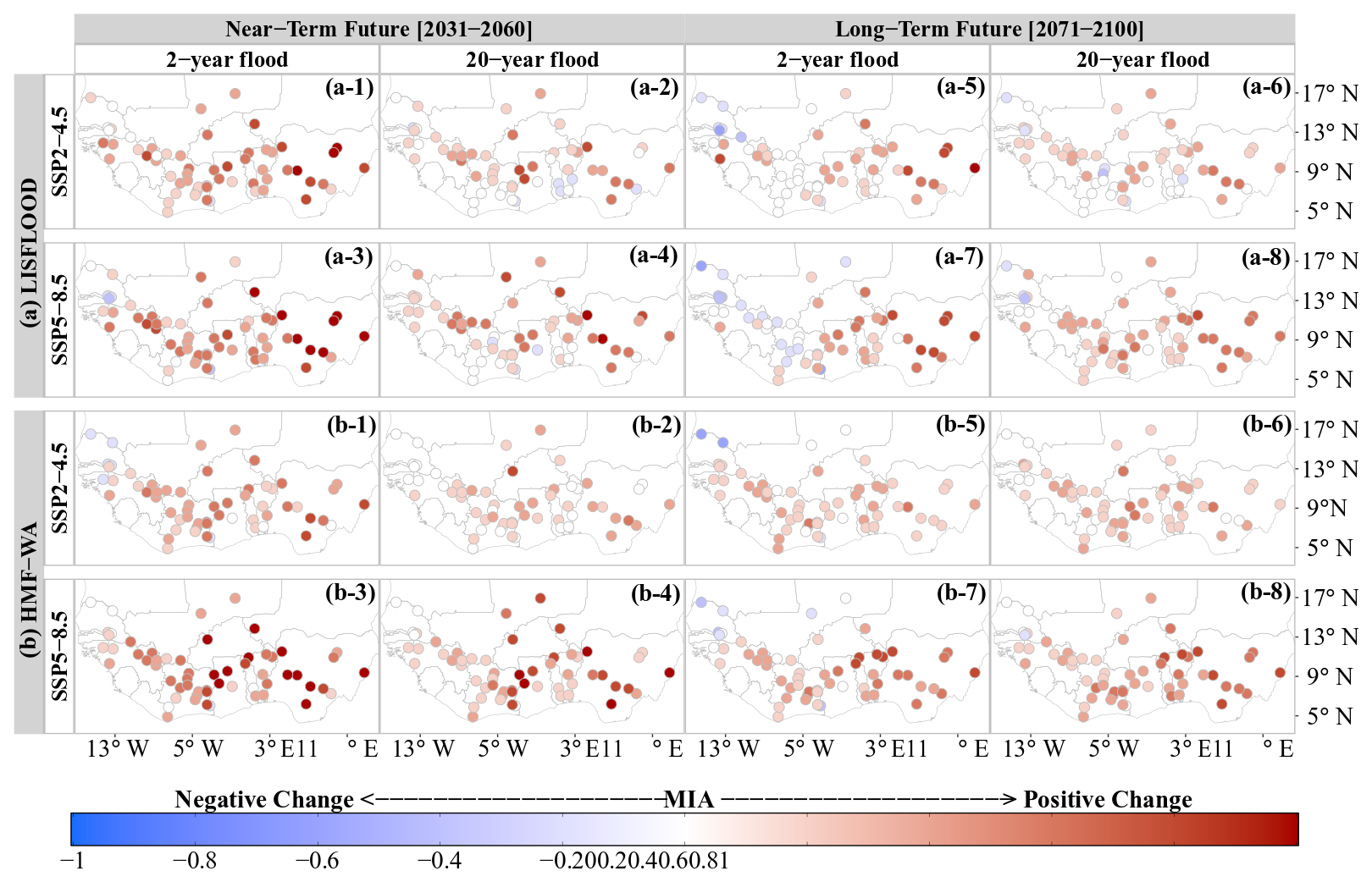
Figure 4 Spatial distribution of the multi-model index of agreement (MIA) on the direction of changes in 2- and 20-year flood events for the near-term (2031–2060) and long-term (2071–2100) futures compared to the historical reference period (1985–2014). This analysis combines simulations from (a) LISFLOOD and (b) HMF-WA hydrological models forced with five bias-corrected CMIP6 models (GFDL, IPSL, MPI, MRI, and UKESM) under the SSP2.4-5 (a-1 to a-4 and b-1 to b-4) and SSP5.8-5 (a-5 to a-8 and b-5 to b-8) scenarios. Flood quantiles are estimated using the GEV distribution fitted with the GMLE method. Negative change (decrease in flood quantiles) is represented by shades of blue, and positive change (increase in flood quantiles) is represented by shades of red.

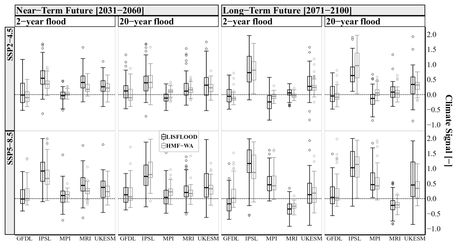
Figure 5 Synthesis of the projected changes in the 2- and 20-year floods in West Africa from the LISFLOOD (black boxplots) and HMF-WA (gray boxplots) model simulations forced with the five CMIP6 GCMs (GFDL, IPSL, MPI, MRI, and UKESM), under the SSP2-4.5 (top row) and SSP5-8.5 (bottom row) climate scenarios for the near-term (2031–2060) and the long-term (2071–2100) futures. The climate signal (y axis) refers to the relative change in flood magnitude, computed as the difference between the future flood quantile (Qfuture) and the historical flood quantile (Qhist), normalized by Qhist. The dotted black line represents the zero-change baseline.

3 Results and discussion

3.1 Assessing the performance of hydrological models

The two hydrological models' performance is assessed over the period of 1950–2014 by applying the two-sample Anderson–Darling (AD) test. The results of the statistical evaluation of the two hydrological models are shown in Fig. 2. The performance of each model at each station is assessed based on the proportion of CMIP6 models that fail the Anderson–Darling test at the 0.05 significance level. Specifically, if more than two out of five CMIP6 simulations fail the test at a given station, the hydrological model is considered to perform poorly at that station. Considering this evaluation criterion, the LISFLOOD hydrological model performs well at 64 % of the stations, while the HMF-WA model performs satisfactorily at only 24 % of the stations (Fig. 2). Although both models are semi-physically based and are spatially distributed, the LISFLOOD model outperforms the HMF-WA model in simulating extreme flows in West Africa (Fig. 2). These findings are consistent with those of Ekolu et al. (2025), who reported that the LISFLOOD model effectively simulates the hydrological cycle and captures the specific characteristics of hydrological droughts and floods in West Africa. This difference in performance can be attributed to several factors: (i) the LISFLOOD model was run at a finer resolution (0.05° × 0.05°) compared to the coarser resolution of 0.1° × 0.1° used by the HMF-WA model (Rameshwaran et al., 2021); (ii) the HMF-WA model includes fewer meteorological forcings and only a limited number of hydrological processes (specifically wetlands, anthropogenic water use, and endorheic rivers), whereas the LISFLOOD model can incorporate over 70 different processes depending on the target application (i.e., rainfall–runoff transformation, flood and drought forecasting) and the required level of configuration (more detailed information on the configuration of LISFLOOD can be found at https://ec-jrc.github.io/lisflood-model (last access: 4 September 2025); and (iii) the HMF-WA model has not been calibrated to individual West African catchment conditions with observed flow data, and its performance depends on the accuracy of the spatial datasets of physical and soil properties (e.g., wetlands, anthropogenic water use, and endorheic rivers) used to configure the model's hydrology to local conditions (Rameshwaran et al., 2021). In contrast, the LISFLOOD model has been regionally calibrated using in situ discharge observations, with discharge time series spanning at least 4 years after 1 January 1982. Consequently, while the distributed nature of the HMF-WA model aims to improve the understanding of regional climate change impacts in a spatially coherent manner across West Africa, it does not necessarily lead to better modeling of extreme flows in the various climates and socioeconomic contexts of the region without calibration. Runoff generation is inherently a spatially distributed process. As such, the spatial resolution of a distributed hydrological model can significantly affect its ability to capture spatial variability in key watershed characteristics, such as topographic features, land cover heterogeneity, and precipitation gradients (Wolock and Price, 1994; Haddeland et al., 2002). A coarser spatial resolution limits the level of detail that can be represented in hydrological simulations, potentially overlooking important small-scale processes. Furthermore, as hydrological models are simplified representations of complex watershed processes, a calibration phase is often necessary to compensate for limited information on spatial variability in physiographical and meteorological catchment attributes and to improve model performance when simulating the watershed's hydrological cycle (Bruneau et al., 1995). However, many river basins in West Africa have a limited number of in situ observational networks to provide the current state of hydrological information (Ndehedehe, 2019). This limits the optimal parameterization of large-scale hydrological models and may introduce uncertainties in model outputs. In addition, the satisfactory performance of the LISFLOOD model indicates that, although a flood-centered calibration approach could potentially improve its ability to capture extreme flows and their trends (Wasko et al., 2023), the current model setup provides a satisfactory basis for regional-scale flood trend assessments.

To further assess the performance of the hydrological models at capturing extreme flows, we computed the relative bias between the AMF simulated by the LISFLOOD-CMIP6 and HMF-WA-CMIP6 hydrological models and the observed AMF from the ADHI database. This comparison was performed over the historical period (1950–2014), focusing on the climatological characteristics of AMF (median values) rather than on year-to-year correspondence. This approach allows us to evaluate whether the hydrological models tend to overestimate or underestimate flood peaks, considering climate models individually. As shown in Fig. 3, the HMF-WA model consistently shows a negative relative bias across all GCMs, with median values ranging from −52 % (IPSL) to −46 % (UKESM) across the region. These negative biases suggest a tendency of the HMF-WA model to underestimate peak flow. The LISFLOOD model, in contrast, shows lower bias than the HMF-WA model, with a mix of slight underestimations and even overestimations (Fig. 3). For instance, the median values for the LISFLOOD model simulations range from −14 % (MPI) to 7 % (GFDL). Although the LISFLOOD model also shows negative biases with most GCMs, such as IPSL, MPI, MRI, and UKESM, the magnitude of these biases is much smaller compared to in the HMF-WA model. Nevertheless, whether a calibrated hydrological model offers more reliable climate change projections than an uncalibrated model, which may perform less accurately at reproducing historical conditions (Pechlivanidis et al., 2017), remains questionable. Examining whether their capacity to simulate hydrological responses to historical climate is influencing projected trends for climate change impacts remains important, especially considering the fact that most projections of climate change impacts on African hydrological trends were produced using uncalibrated models (Davie et al., 2013; Sauer et al., 2021).

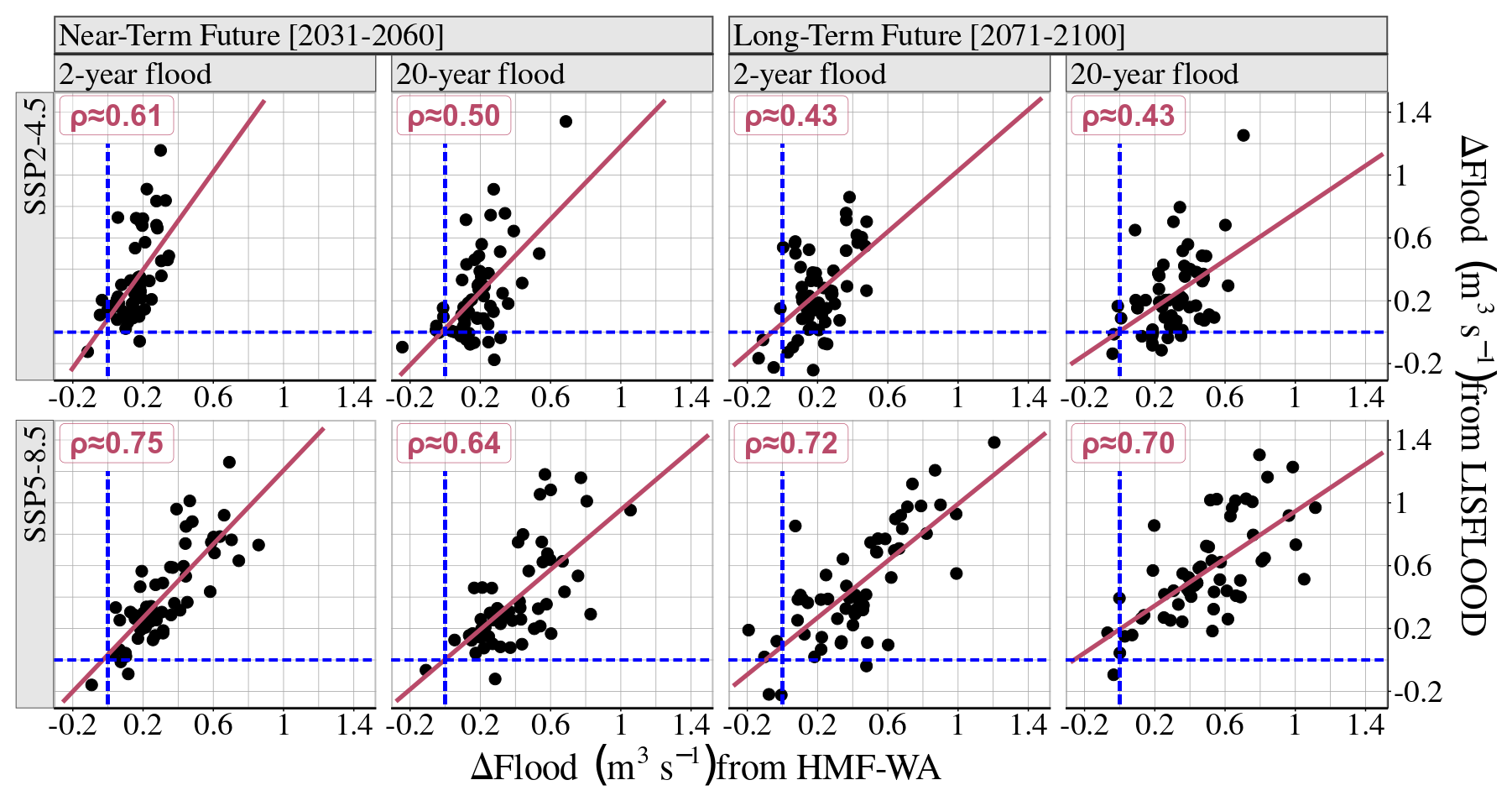
Figure 6 Comparison of projected multi-model mean changes in flood (Δ flood) between the LISFLOOD and HMF-WA hydrological models under the SSP2.4-5 (top row) and SSP5.8-5 (bottom row) scenarios for the near-term (2031–2060) and the long-term futures (2071–2100) compared to the historical reference period (1985–2014). The dashed blue lines represent the zero-change baseline, and the red diagonal line represents the theoretical 1:1 line where projected changes from both hydrological models would be identical.

3.2 Magnitude and direction of changes in flood events

To analyze changes in floods, we have compared two 30-year future periods (a near-term future (2031–2060) and a long-term future (2071–2100)) to a reference historical period (1985–2014). To achieve this, we have fitted the GEV distribution to the AMF series of each model simulation using the GMLE method. Then, the 2- and 20-year flood quantiles are computed at each station for the three 30-year periods. Figure 4 shows the MIA on the direction of changes in the 2- and 20-year floods for the near-term and long-term futures from both LISFLOOD and HMF-WA model simulations under the SSP2.4-5 and SSP5.8-5 scenarios. Despite their differences in terms of hydrological process representation (model structures) and input data, the two hydrological models generally projected consistent impacts of climate change on future floods across the West African region. Both hydrological models consistently project an increase (positive change) in floods in the near-term and long-term futures across West Africa (Fig. 4).

In the near-term future (2031–2060), there is a high level of agreement when projecting positive changes in the 2-year flood event under both the SSP2-4.5 and SSP5-8.5 scenarios. The simulations of the LISFLOOD and HMF-WA models show strong agreement across the CMIP6 models. Under SSP2-4.5, the MIA values range from −0.2 to 1 for the LISFLOOD model (Fig. 4a-1) and from −0.2 to 0.8 for the HMF-WA model (Fig. 4b-1). This agreement increases for both hydrological models under SSP5-8.5, with MIA values falling between −0.2 and 1 for both the LISFLOOD (Fig. 4a-3) and HMF-WA models (Fig. 4b-3). The consistent climate change impact projections suggest that more frequent flood events are expected to become increasingly common across the West African region. For the 20-year flood event, which is less frequent but more severe, MIA values range from −0.2 to 0.8 (−0.2 to 1) and from 0 to 0.8 (0 to 1) under SSP2-4.5 (SSP5-8.5) for the LISFLOOD (Fig. 4a-2 and a-4) and HMF-WA (Fig. 4b-2 and-4) models, respectively.

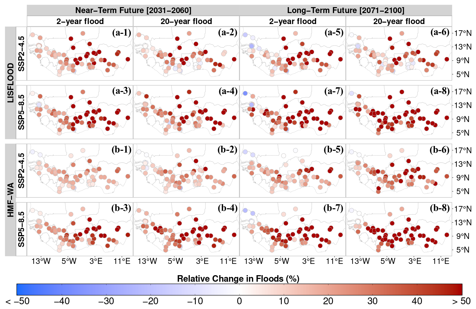
Figure 7 Mean relative changes in the 2- and 20-year floods in West Africa for the near-term (2031–2060) and long-term (2071–2100) futures based on simulations from the LISFLOOD (a-1 to a-8) and HMF-WA (b-1 to b-8) hydrological models under SSP2-4.5 and SSP5-8.5 scenarios.

In the long-term future (2071–2100), considering the 2-year flood, MIA values range from −0.6 to 1 (−0.6 to 0.8) and from −0.6 to 0.6 (0.4 to 0.8) under SSP2-4.5 (SSP5-8.5) for the LISFLOOD (Fig. 4a-5 and a-7) and HMF-WA (Fig. 4b-5 and b-7) models, respectively. For the 20-year flood, model agreement in projecting the positive changes in flood magnitude remains relatively high, with MIA values ranging from −0.4 to 0.6 (−0.4 to 0.8) and from 0 to 0.6 (−0.2 to 0.8) under SSP2-4.5 (SSP5-8.5) for the LISFLOOD (Fig. 4a-6 and a-8) and HMF-WA (Fig. 4b-6 and b-8) models, respectively. It is also worth noting that negative changes are projected in the 2-year flood in the long-term future in a few sets of catchments located in the western part of the region (Fig. 4a-5, a-7, b-5 and b-7). This area is also projected to experience a decrease in annual rainfall when looking at the full CMIP6 ensemble (IPCC, 2021). However, the agreement between the CMIP6 models remains very weak, indicating lower confidence in the robustness of these negative changes compared to the regional pattern. Overall, the agreement between the CMIP6 and the hydrological models is higher for the near-future than for the long-term future, reflecting increased uncertainty as the projection timeline extends.

Figure 5 summarizes the projected climate impacts on floods in the near-term (2031–2060) and long-term (2071–2100) futures in West Africa across the different CMIP6 models (GFDL, IPSL, MPI, MRI, and UKESM). Both hydrological model simulations consistently suggest strong changes in floods, with most median values falling above the zero-change baseline. Considering the CMIP6 model projections individually in the near-future, under both the SSP2-4.5 (Fig. 5a) and SSP5-8.5 (Fig. 5b) scenarios, the most pronounced changes are obtained for both hydrological models when forced with the IPSL, MRI, and UKESM models. These near-term projections highlight the potential for more frequent extreme flood events, leading to increased flood risks and greater socioeconomic vulnerability in the West African region. In the long-term future, the distribution of flood trends is quite consistent between the two hydrological models, and the variability stems only from GCMs. For instance, under SSP2-4.5, the variability between the different CMIP6 models is very pronounced, with most projections showing relatively modest changes compared to the SSP5-8.5 scenario, where most of the GCMs agree on a positive change in flood magnitudes.

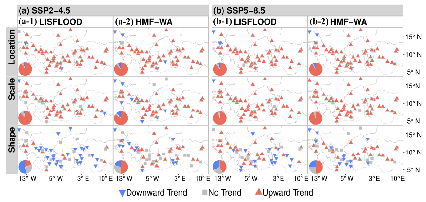
Figure 8 Direction of significant trends detected using the Mann–Kendall trend test (at the 0.05 significance level) for GEV parameters: location (top row), scale (middle row), and shape (bottom row). The GEV parameters are estimated based on multi-model mean streamflow over 30-year moving windows. Panels (a-1) and (b-1) display the results for the LISFLOOD model under SSP2-4.5 and SSP5-8.5, respectively, while panels (a-2) and (b-2) show the results for the HMF-WA model under SSP2-4.5 and SSP5-8.5, respectively. The red upward triangles indicate significant upward trends, and the blue downward triangles indicate significant downward trends, both at the 0.05 significance level. Gray rectangles represent cases where no significant trends are detected. The pie charts summarize the proportion of stations showing significant positive trends (red), significant negative trends (blue), and non-significant trends (gray).

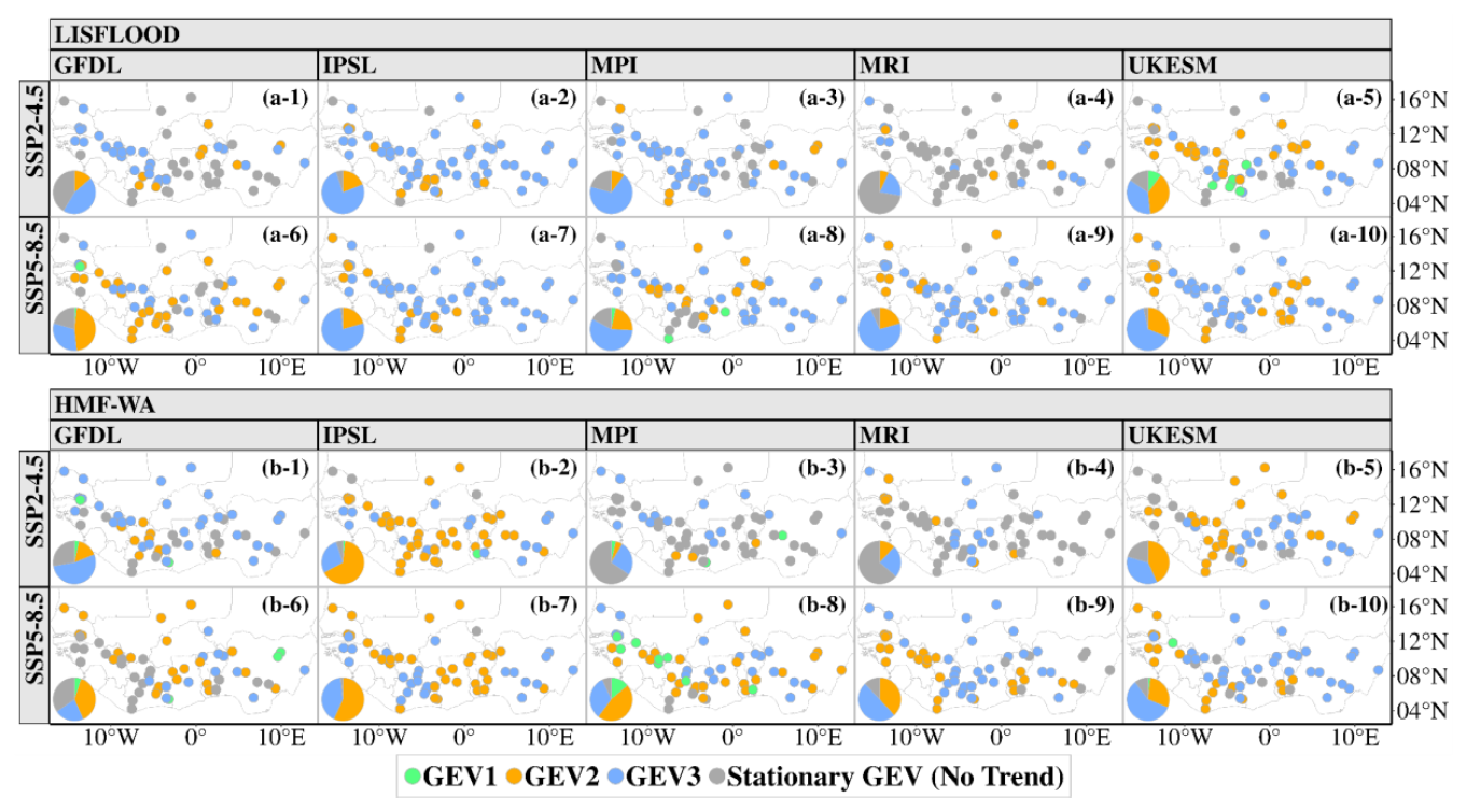
Figure 9 Best-fitting GEV trend models at each station, determined using the AIC criterion and the deviance test based on simulations from (a) LISFLOOD-CMIP6 (top rows) and (b) HMF-WA-CMIP6 (bottom rows) under the SSP2-4.5 and SSP5-8.5 scenarios. The green points represent stations best modeled by GEV1, which assumes a linear trend over the entire record. The orange points indicate stations best modeled by GEV2, which assumes stationarity before a breakpoint followed by a linear trend after the breakpoint. The blue points denote stations best modeled by GEV3, which assumes a double linear trend. The gray points represent stations where all non-stationary GEV models are rejected based on the deviance test. The pie charts summarize the proportion of stations at which the stationary GEV model (gray) or one of the non-stationary models, GEV1 (green), GEV2 (orange), or GEV3 (blue), is identified as the best suited to fit the AMF series.

To further assess the agreement between the two hydrological models, Fig. 7 displays how the projected multi-model mean changes in floods (Δ flood) compares between the LISFLOOD and HMF-WA model simulations. Overall, both models project positive change in floods in West Africa regardless of the SSP scenario considered. Indeed, most data points fall above the zero-change baseline, indicating a global positive change in floods from both hydrological model simulations (Fig. 7). To confirm the agreement between the two models, we have computed the Spearman coefficient (ρ) between Δ flood from the simulations of the LISFLOOD and HMF-WA models. The correlation analysis shows that the agreement between the two models is particularly pronounced under the SSP5-8.5 scenario, suggesting a stronger influence of climatic changes under the high-emissions scenario. In the near-term future, the Spearman correlation coefficient is 0.75 (0.64) for the 2-year (20-year) floods. In the long-term future, the correlation remains high, with 0.72 (0.70) for the 2-year (20-year) floods, suggesting that the models continue to show strong agreement, even in long-term projections. These results indicate a relatively high level of consistency between the two hydrological models when projecting future flood changes, despite the systematic biases in HMF-WA model over the reference historical period. Thus, when using both models, the climate forcing has more importance than the hydrological representation itself.

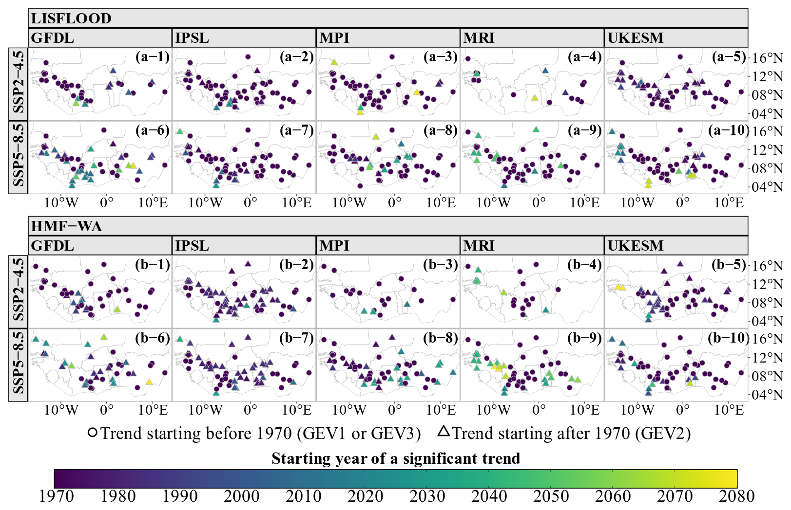
Figure 10 Spatial distribution of the starting years of significant flood trends projected by (a) LISFLOOD and (b) HMF-WA hydrological models forced with CMIP6 models (GFDL, IPSL, MPI, MRI, and UKESM) under the SSP2-4.5 and SSP5-8.5 scenarios. The color gradient indicates the starting year of a significant flood trend, ranging from 1970 (purple) to 2070 (yellow). Circular markers represent sites where trends began at the start of the time series (before 1970). Triangular markers indicate sites where trends emerged after 1970 (the linear trend GEV2 case).

The relative magnitude of change in floods was also analyzed by computing the mean relative change. (i.e., the ratio of the difference between the flood quantiles of the future periods and the reference historical period) across CMIP6 models for each hydrological model. The spatial distribution of the magnitude of changes, as simulated with the LISFLOOD and HMF-WA hydrological models under both SSP2-4.5 and SSP5-8.5, is shown in Fig. 7a and b. Table S3 in the Supplement summarizes the overall mean relative change in floods across the region from both hydrological model simulations. The two hydrological models consistently project an increase in future floods across the West African region, with flood magnitudes at most sites exceeding 50 %, particularly under SSP5-8.5 (Fig. 7a-3, a-4, a-7, a-8, b-3, b-4, b-7, and b-8). These results are consistent with previous studies that argued for the ongoing rising trend in extreme streamflow across the West African catchments (Nka et al., 2015; Aich et al., 2016; Wilcox et al., 2018; Ekolu et al., 2025). However, a common limitation of most previous studies is their reliance on a relatively small sample of watersheds and their limited spatial coverage, which may overlook local hydrographic variability and limit regional applications. In addition, most impact studies in West Africa are based on conceptual hydrological models at catchment scales. The study differs from previous studies by covering an unprecedented set of catchments and by utilizing state-of-the-art bias-corrected CMIP6 climate models, two large-scale hydrological models, and robust statistical methods to assess both the magnitude and field significance of future flood changes. As such, the findings from this work provide regional-scale insights into the evolving flood risks in West Africa. Furthermore, the findings from the studies of Almazroui et al. (2020), Dosio et al. (2021), and Dotse et al. (2023) have shown that CMIP6 models contain a robust signal of the intensification of the rainfall regime in West Africa. The increasing trend in floods across the region may be partly explained by the trends in extreme precipitation, as their variability influences the hydrological dynamics of the region (Panthou et al., 2013; Wilcox et al., 2018; Elagib et al., 2021).

3.3 Onset of changes in AMF series

3.3.1 Observed trends in GEV parameters

As the climate and environment change (Lee et al., 2023), it is essential to examine how these changes affect the parameters of GEV distributions. Figure 8 shows the spatial distribution of trends detected by the Mann–Kendall test on GEV parameters estimated on multi-model mean AMF over 30-year moving windows from 1950 to 2100. Both hydrological models project upward trends in the location and scale parameters across the West African region, with a strong agreement between the two hydrological models (see Fig. 8). All local trends are field significant at the 0.05 level according to the FDR procedure. The simulated upward trends in both parameters observed across various watersheds and emission scenarios emphasize the importance of accounting for temporal variability in GEV parameters to reliably model future flood risks. An increase in the location parameter suggests more frequent and severe floods, while an upward trend in the scale parameter indicates greater variability in flood magnitudes. In contrast, the “mixed” trends observed in the shape parameter, with no distinct spatial patterns, support the decision to model it as constant over time, as there is no strong regional evidence of consistent temporal changes in its behavior across the region.

3.3.2 Selection of the best-suited GEV trend model

Using non-stationary GEV models, we analyze temporal shifts in floods by fitting time-dependent GEV parameters to the AMF series from both hydrological model simulations. To detect the onset of significant trends in flood events, we have allowed any starting year (t0) of a possible trend in the GEV location μ(t) and scale σ(t) parameters between 1970 and 2070. To select the best non-stationary GEV model for each site, we have compared the goodness of fit of three different time-varying GEV models. The models evaluated are (1) a linear trend for both the μ(t) and σ(t) parameters without a breakpoint (GEV1), (2) a linear trend for μ(t) and σ(t) starting after a specific breakpoint (GEV2), and (3) linear trends for μ(t) and σ(t) both before and after a breakpoint (GEV3). Figure 9 shows the GEV trend model selected at each station according to the AIC criterion and the deviance test for the LISFLOOD-CMIP6 and HMFWA-CMIP6 simulations under both the SSP2-4.5 and SSP-8.5 scenarios. Although both hydrological models project an increase in floods (Fig. 5), they simulate slightly different trend patterns across the study area. Considering the LISFLOOD model (Fig. 9a), the GEV3 (double-linear trend) is consistently best suited at most stations, with high agreement between the CMIP6 models. For instance, under the SSP2-4.5 scenario, the GEV3 distribution outperforms other models at 66 %, 79 %, and 76 % when the LISFLOOD model is driven by the GFDL (Fig. 9a-1), IPSL (Fig. 9a-2), and MPI (Fig. 9a-3) climate models, respectively. A similar trend is observed under SSP5-8.5, where the GEV3 is best suited when LISFLOOD is forced with the MPI (62 %), MRI (77 %), IPSL (78 %), and UKESM (66 %) models (Fig. 9a-7, a-8, a-9 and a-10). The HMF-WA simulations show a mixed spatial pattern between the GEV2 and GEV3 models (Fig. 9b). For both hydrological models, the single linear trend model (GEV1) is selected at very few stations (less than 5 %). Meanwhile, the stationary behavior observed at a few sites under SSP2-4.5 suggests that certain river basins may experience little to no change in their hydrological extremes under moderate emissions pathways.

3.3.3 Starting years of trends in flood hazards

The spatial distribution of the starting years of significant flood trends detected with the GEV trend models are shown in Fig. 10. The projections from the two hydrological models are spatially coherent, and the temporal variability in the start of flood trends in the region seems to depend on climate models. Overall, under both SSP2-4.5 and SSP5-8.5, the majority of significant trends are identified on almost the whole record from the 1980s onward, in agreement with long-term trends observed in this region (Tramblay et al., 2020), particularly with the GFDL, IPSL, MPI, and UKESM models. This consistent pattern of early starting years suggests that West African communities are already facing high flood risks and are likely to experience exacerbated conditions in the near future. For the two linear trends in the GEV3 model, as shown in Fig. S5 in the Supplement, the predominant spatial pattern is a transition from decreasing flood trends before the breakpoint to increasing trends after. Persistent increases, characterized by positive slopes before and after the breakpoint, are also observed at several sites, particularly with the GFDL, IPSL, and UKESM climate models.

4 Conclusions

This study has assessed the regional-scale hydrological impacts of climate change in West Africa, specifically focusing on floods, from two large-scale hydrological models (HMF-WA and LISFLOOD) driven by five bias-corrected CMIP6 climate models under the SSP2-4.5 and SSP5-8.5 scenarios. A multi-model index of agreement (MIA) was used to assess the robustness of the projections from the hydrological model. The statistical evaluation of the two hydrological models, performed using the two-sample Anderson–Darling test between the annual maximum flows observed from the ADHI database and those simulated by the hydrological models, revealed that the LISFLOOD model outperforms the HMF-WA model in simulating extreme flows in West Africa. The GEV distribution was used to analyze trends and detect change points by fitting and comparing multiple GEV models to the AMF series, covering both the historical and future periods. Two 30-year future periods (a near-term future (2031–2060) and a long-term future (2071–2100)) were compared to a reference historical period (1985–2014). Despite differences in hydrological process representations, model architecture, and calibration, the two hydrological models generally projected consistent impacts of climate change on future floods across the West African region with a relatively high level of consistency. This agreement between the two hydrological models suggests that the climate forcing has more importance than the hydrological representation itself, and un-calibrated models can provide reliable scenarios in this region. An increase in floods (2 and 20 year) is observed at more than 94 % of the stations, with some locations experiencing flood magnitudes exceeding 45 %. The results of the comparison between GEV trend models show that the double-linear-trend GEV model, with both location and scale parameters expressed as being time dependent, is best suited for most stations. The analysis of the starting years of significant flood trends revealed that most shifts in extreme flood patterns occurred early in the time series, as early as the 1970s in several basins.

The use of the GCM outputs to drive hydrological models introduces uncertainties to hydrological simulations. Indeed, the outputs of general circulation models (GCMs) are characterized by uncertainties arising from several factors. such as the simplified representation of complex-Earth-system interactions and atmospheric processes, the uncertain socioeconomic pathways, the coarse spatial resolution of these models, and the challenges related to model parameterization (Hawkins and Sutton, 2009). In addition, the performance of large-scale hydrological models is influenced by the driving inputs, the representation of the hydrological process, and the model parameterization (Andersson et al., 2015). Current models also have difficulties reproducing hydrological processes in arid regions (Heinicke et al., 2024). It would therefore be interesting to explore in more detail the main sources of uncertainties in hydrological projections in West Africa to improve the realism of such modeling approaches in the future.