Reask UTC: a machine learning modeling framework to generate climate-connected tropical cyclone event sets globally

In the early 1990s, the insurance industry pioneered the use of risk models to extrapolate tropical cyclone (TC) occurrence and severity metrics beyond historical records. These probabilistic models rely on past data and statistical modeling techniques to approximate landfall risk distributions. By design, such models are best fit to portray risk under conditions consistent with our historical experience. This poses a problem when trying to infer risk under a rapidly changing climate or in regions where we do not have a good record of historical experience. We here propose a solution to these challenges by rethinking the way TC risk models are built, putting more emphasis on the role played by climate physics in conditioning the risk distributions. The Unified Tropical Cyclone (UTC) modeling framework explicitly connects global climate data to TC activity and event behaviors, leveraging both planetary-scale signals and regional environment conditions to simulate synthetic TC events globally. In this study, we describe the UTC framework and highlight the role played by climate drivers in conditioning TC risk distributions. We then show that, when driven by climate data representative of historical conditions, the UTC is able to simulate a global view of risk consistent with historical experience. Additionally, the value of the UTC in quantifying the role of climate variability in TC risk is illustrated using the 1980–2022 period as a benchmark.

1 Introduction

Tropical cyclones (TCs) pose a threat to coastal communities across the globe. Recent examples include a record-breaking 2022 season for Madagascar, where five storms made landfall, causing up to 365 fatalities across Madagascar, Mozambique, and Malawi (Aon, 2022). Sadly, these regions were impacted again in 2023 by category 5 TC Freddy, causing up to 3 times more fatalities. From an economic stand point, TCs caused USD 92 billion of global economic losses in 2021, with Hurricane Ida alone costing USD 75 billion (Aon, 2021), while in 2022, category 5 Hurricane Ian became the third-costliest event on record, with over USD 100 billion of economic losses (Smith, 2020). At the time of writing, hurricanes Helene and Milton have just hit the west coast of Florida, with combined expected economic losses in excess of USD 50 billion (Morningstar, 2024).

A range of public and private organizations focus on mitigating this risk. To do so, they require tools that quantify the occurrence and severity likelihood of events globally. Since the early 1990s, the insurance industry has adopted the use of large sets of synthetic TC events as a way to understand and quantify TC risk beyond simple analysis of historical records. These synthetic events all represent plausible TC scenarios, typically generated from statistical extrapolation of historical occurrences (Hall and Jewson, 2007; Rumpf et al., 2007; Vickery et al., 2009; Bloemendaal et al., 2020; Arthur, 2021). The climatology and statistics of such event sets (often referred to as stochastic event sets in reference to their generation process) are consistent with history but allow extrapolation beyond what was observed. They help quantify probabilistic measures of risk such as the 1-in-100-years return period hazard intensity (i.e., an intensity level with a 1 % annual chance of occurrence).

While such methods have greatly helped the industry better understand TC risk, they suffer from a fundamental limitation: they are mostly driven by statistics of past data rather than physics. At the core of the event generation process resides a series of statistical relationships that are fit to historical data and therefore best represent TC risk under conditions that are consistent with historical data points. This presents two important challenges when assessing global risk in a changing climate:

• A model anchored in past climate conditions is not able to adapt and quantify shifts in risks associated with a changing climate. For example, how do TCs react to regional changes in patterns of dominant atmospheric steering flow, ocean temperatures, or wind shear?

• A model fit to historical data will be best fit to those regions where we have abundant historical records (e.g., the North Atlantic) but will generalize poorly to other basins where data are scarce and TC behaviors may differ (e.g., the South Indian Ocean).

One solution to this problem is to build smarter event generation algorithms that do not simply memorize and extrapolate history but also understand how climate physics influenced the observed outcomes. Explicitly linking the event generation algorithms to key climate drivers allows the creation of climate-connected event sets that can naturally quantify risk (1) under changing climate conditions and (2) in regions where historical data are scarce. Several climate-connected TC event sets have recently been developed by the academic community, with leading modeling groups developing TC risk solutions that explicitly link some components of the event generation process to climate model outputs (Lee et al., 2018; Jing and Lin, 2020; Emanuel, 2021, and citations within; Lin et al., 2023; Sparks and Toumi, 2024). We here present a novel approach (the Unified Tropical Cyclone – UTC) that, while following a similar philosophy, differs in several key aspects:

• The UTC links the annual frequency of TC occurrence in each active basin to large-scale environment signals (e.g., El Niño–Southern Oscillation – ENSO) rather than through the use of more localized genesis potential indices (e.g., TCGI; see Wang and Murakami, 2020).

• The UTC directly simulates the impact of sea surface temperatures, atmospheric steering flow, mean sea level pressure, and vertical wind shear on the TC trajectory and intensity hourly increment distributions thanks to a machine learning (ML) algorithm called quantile regression forest (Meinshausen, 2006; Loridan et al., 2017; Lockwood et al., 2024; Bruneau et al., 2024). Using ML ensures that the impact of local environmental factors can be inferred directly from data without the need for any expert judgment in formulating or tuning the relationship.

• The UTC is initialized with reanalysis data and model simulations of the past (see the results of this study below) but also with seasonal forecast data and future climate projections (this will be the focus of a follow-up study). Figure 1 provides an introductory illustration of how the UTC risk distributions (here for annual major hurricane US landfalls) shift according to different climate forcing conditions. More details on this experiment are provided in Sect. 3.

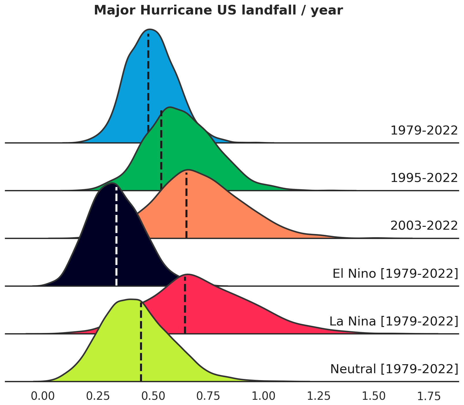
Figure 1 UTC modeled distributions of annual US major hurricane landfalls, under a range of climate forcing assumptions. Vertical dashed lines show observed levels of occurrence for each scenario.

In this study, we describe how climate gridded data are used to condition the UTC event generation algorithms, namely, the TC occurrence frequencies by basin, genesis location, date, track trajectory, and intensity modules. We then show how such a climate-connected approach can reproduce a risk climatology across the globe that is consistent with history, with minimal need for local tuning, track filtering or calibration. We then conclude by analyzing the impact of climate variability on the UTC view of risk, considering alternative climates of the 1980–20222 period as forcing when deploying the model.

2 The Unified Tropical Cyclone (UTC) modeling framework

The UTC framework consists of a series of algorithms that allow generation of synthetic events from knowledge of global climate conditions (Fig. 2). By generating a large number (i.e., millions) of such climate-connected synthetic events, we aim to capture a complete view of TC risk under the climate conditions provided as input. An overview of the event generation framework is first provided in Sect. 2.1. Section 2.2 details how the event generation algorithms are developed, combining reanalysis of past climate with historical TC event records. In Sect. 2.3, we come back to the event generation framework and formally list the sequence of algorithmic steps that make up the UTC.

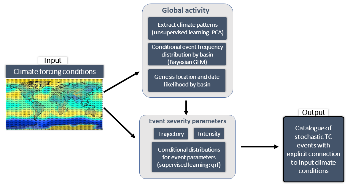
Figure 2 Overview of the UTC event generation framework. Global gridded climate data are used as input to a series of algorithms responsible for the generation of synthetic TC events. The output is a set of millions of events, representative of TC activity under conditions set by the input climate data. Details of the algorithms are provided in Sect. 2.2 and Appendix A1.

2.1 Event generation framework overview

The overarching objective when creating a climate-connected TC event set is to sample two dimensions of risk variability (see Fig. 1):

• A) the variability in TC risk under a given climate state (the distribution in each row of Fig. 1).

• B) the variability in the climate state itself (different rows in Fig. 1).

While most traditional TC event sets are designed to address A (for a climate representative of a selected historical average state, e.g., first row of Fig. 1), they fail to acknowledge the importance of B. To address B and drive the generation of events covering a wide range of climate conditions, we connect the UTC to global gridded climate inputs: ERA5 (Hersbach et al., 2020) is our preferred source to portray the climate experienced historically, and we also augment that view with alternative simulated climates from the CESM LENS2 project (Rodgers et al., 2021). While ERA5 data are available at higher resolution, we choose to aggregate to a similar 1° spatial resolution as the CESM LENS2 data. This choice is driven by a desire for consistency between model training (with ERA5) and deployment (using a wider range of sources not always available at the same resolution as ERA5, such as the CESM LENS2). When representing the climate state at 1° spatial resolution, we focus on variability in global and regional climate patterns rather than finer-scale weather. In this framework, the sampling of risk due to finer-scale weather variability is part of dimension A above. This large database of monthly global gridded climate data is the starting point for our model deployment (Fig. 2). We limit the range of climate inputs to state variables that are known to impact TC dynamics:

• Sea surface temperature (SST)

• Mean sea level pressure (MSLP)

• Zonal component of the wind flow at 850 mbar (U850) and 200 mbar (U200)

• Meridional component of the wind flow at 850 mbar (V850) and 200 mb (V200)

• Vertical wind shear magnitude (SHR) – computed from the wind field components above

• Steering flow – also computed from the wind field components.

The UTC then implements the following modeling sequence (see Fig. 2):

1. A climate state is defined as a time series of monthly gridded climate data fields. From knowledge of key climate patterns in a given climate state (see Sect. 2.2.1), the UTC models one distribution per basin to define event count likelihood during a TC season experiencing that climate (Sect. 2.2.2). This process is repeated for a large number of climate states to capture dimension B described above.

2. Within each climate state, hundreds of different sample years (stochastic years) are computed to capture dimension A. These stochastic years account for variability in finer-scale climate conditions (e.g., weather) not captured by the coarse climate forcing, as well as other stochastic TC behaviors occurring under a given climate state. For each stochastic year, and from knowledge of the distributions in 1, a number of events (nTC) per basin is sampled to define TC activity for that year.

3. For each of the nTC events sampled in a stochastic year, a likely genesis date and location are sampled from knowledge of historical occurrence rates and local environment conditions (Sect. 2.2.3).

4. For each sampled event, the UTC simulates the trajectory of the TC center at 1 h intervals, taking into account track persistence and the effect of environmental conditions such as the steering flow (Sect. 2.2.4).

5. Simultaneously, the evolution of the TC intensity (center pressure) is also sampled along the track at 1 h intervals, from knowledge of the track characteristics to date and environmental conditions such as the vertical wind shear and ocean temperatures (Sect. 2.2.5). An estimate of maximum sustained winds at 10 m is also computed from the modeled TC center pressure following Bruneau et al. (2024).

By repeating the steps above for a large number of climate states (i.e., many years of climate forcing in 1) and a large number of stochastic samples (i.e., repeated sampling of 2), the UTC generates a set of events characterizing risk variability across dimensions A and B.

With a complete record of the climate states used to generate any of the stochastic years, the UTC framework opens up a whole new range of analysis around the impact of climate variability (e.g., Fig. 1). By grouping years according to the phase of the El Niño–Southern Oscillation (ENSO), one can, for instance, quantify the resulting shifts in likelihood of TC landfalls across the world, along with potential correlations between basins/regions. Similarly, questions around the impact of already realized warming of the atmosphere on TC activity can be addressed objectively by sub-sampling the event set according to the warming levels of the forcing climate states (e.g., first three rows of Fig. 1). From a risk analysis point of view, the UTC also helps identify regions of the world that may have been lucky/unlucky in their historical experience compared to what should be expected over the period of records (see Sect. 3).

2.2 Event generation algorithms

When training the UTC event generation algorithms, we combine two data sources that jointly capture historical TC risk conditions over the 1980–2020 period (i.e., the model training period):

• Monthly gridded data from the ERA5 reanalysis dataset (Hersbach et al., 2020) provide a best estimate of the climate experienced globally over the period.

• The International Best Track Archive for Climate Stewardship (IBTrACS; Knapp et al., 2010) records the frequency, trajectory, and intensity of TC events globally.

Most of the algorithms described below are based on machine learning (ML), i.e., they derive their form directly from data rather than from a human-selected relationship. Throughout this section, key concepts are illustrated using case studies and simplified algorithms where the physics is easily discussed. The complete algorithms, as implemented in the UTC, are detailed in Appendix A1.

2.2.1 Extracting patterns of climate variability impacting TC activity

The first step in the UTC framework is to reduce the dimension of the raw input of monthly gridded data into a selection of patterns important to TC activity. This dimension reduction phase is done via principal component analysis (PCA, see Appendix A1), performed on a range of standardized anomaly fields (FLD = SST, MSLP, U850, U200, V850, V200, and SHR – see Sect. 2.1).

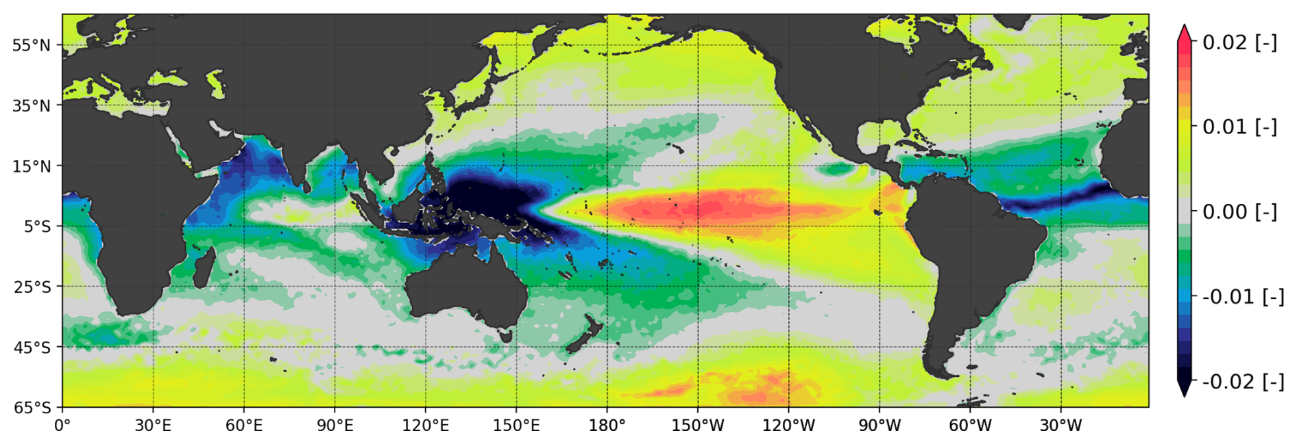
Figure 3 Principal component field representing one of the leading modes of global sea surface temperature variability (PC_SST,3). See Eq. (A1) for details.

The end result for a given field is a series of spatial patterns (PC_FLD,i, see Fig. 3) allowing decomposition of any state of the field using a series of coordinates (W_FLD,i, see Eq. (A1) in Appendix A1). While the PCA step provides important insights into the leading modes of global climate variability for each field (the PC_FLD,i), these are not all equally relevant to TC risk. To filter out the patterns most relevant to TC activity across different basins, we rely on two criteria (Appendix A2):

• Only consider PC_FLD,i modes whose weights (W_FLD,i) correlate with TC activity in at least one basin (candidate PC_FLD,i, see Fig. 4).

• Ensure that the physical reasons for that correlation are understood. This is done by screening the patterns in the candidate PC_FLD,i and explicitly linking them to conditions known to be favorable/unfavorable to TC genesis.

An example of the above is given in Fig. 3 with PC_SST,3 obtained from the SST decomposition of Eq. (A1). The correlation between the number of North Atlantic hurricanes and the associated weights (W_SST,3), averaged over the July–November period, is shown in Fig. 4. The reasons for the (negative) correlation between the magnitude of the weights and North Atlantic hurricane activity can be understood from an analysis of Fig. 3: large values of the W_SST,3 weights are associated with anomalously warm SSTs in the eastern and central Pacific (typical of an El Niño event) and anomalously cold SSTs in the tropical Atlantic. Both trends are signals of a likely weak hurricane season, which is confirmed by Fig. 4. Conversely, large negative values of the weight tend to be associated with La Niña type of Pacific SSTs and an anomalously warm tropical Atlantic, i.e., conditions favorable to hurricane activity.

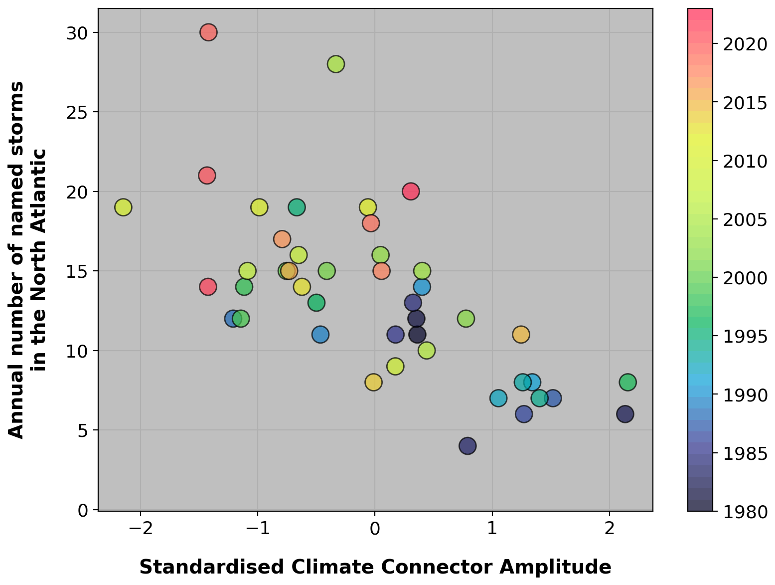
Figure 4 Relationship between the weight associated with the principal component from Fig. 3 (x axis) averaged over the July–November period (i.e., C_NA,1, Appendix A2) and the number of North Atlantic tropical storms in that season (y axis). Colors indicate the season of record. Common statistical evaluation metric for this dataset: R = −0.66; R² = 0.44; p-value: 1.11 × 10⁻⁶.

Altogether a total of 13 patterns (PC_FLD,i) are selected to characterize climate states within the UTC framework (globally). As is the case in the example of Fig. 4, we maximize the correlation from the raw time series of weights by averaging over a time window that covers the peak TC activity period in each basin. The result is a set of 13 scalars that allow conditioning of TC activity in all active basins of the world. In what follows, we refer to these scalars as climate connectors, and the complete list of connectors is provided in Appendix A2.

2.2.2 Conditional distribution of TC numbers given the magnitude of climate patterns

By design, the connectors selected in Sect. 2.2.1 correlate with TC activity in at least one basin. They therefore offer a way to link the input climate state to trends in basin-wide TC numbers. However, a large uncertainty exists around the exact number of TCs to expect under a given climate state (e.g., see vertical spread in Fig. 4 for a given C_NA,1 value).

Our approach to this challenge is to adopt a hierarchical Bayesian modeling framework, similar in concepts to that of Elsner and Jagger (2004). We use the connectors listed in Appendix A2 to condition the λ rate of a Poisson distribution (see Appendix A3). Figure 5 illustrates the end result in a simplified case where the distribution of North Atlantic hurricanes is conditioned only on the value of the average July–November W_SST,3 shown in Fig. 4 (i.e., connector C_NA,1, see Eq. A2).

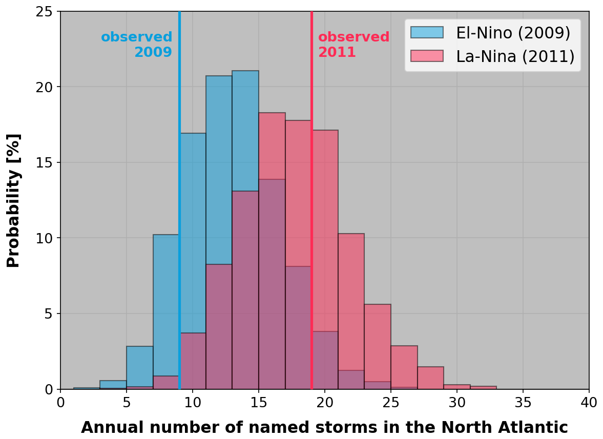
Figure 5 Modeled distribution of hurricane activity conditioned on the value of the average July–November W_SST,3 weight from Fig. 4 for 2009 (blue) and 2011 (red) climates. The vertical lines show observed activity levels in 2009 (El Niño year) and 2011 (La Niña year).

In years with large positive values of the connector (e.g., El Niño years – see Fig. 3) the modeled distribution of hurricane numbers shifts to a less active state (light blue), while for large negative connector values (e.g., La Niña years), the shift is towards more frequent activity (red).

For each basin that is TC active (i.e., North Atlantic, East Pacific, western North Pacific, North Indian, South Indian, and South Pacific basins), we have developed a different hierarchical Bayesian model using between two and three connectors. These are listed in Appendix A3. The ability of this approach to capture variability in TC basin frequency over the 1980–2022 period is illustrated in Sect. 3.1 (see Fig. 10).

To help capture sub-basin spatial variability in TC genesis likelihood, the steps above are repeated to distribute the total number of basin-wide events across a set of sub-regions.

At the scale of each basin:

• A set of sub-regions is defined (see Fig. A1 in Appendix A2), and for each historical season in the 1980–2020 training set, we record the ratio (0–1) of the total basin-wide activity that occurs in the sub-regions.

• The atmospheric fields described in Sect. 2.1 are restricted to each basin domain, before PCA reduction. Resulting PCA fields and weights are recorded for all years in the training set. This allows extraction of patterns of climate variability within each basin.

• The correlation from PCA weights is assessed with regards to each sub-region activity ratio, rather than the absolute TC number. As an example, we find that the third PCA for the stacked SHR + SST + MSLP fields in the North Atlantic is a good predictor of the ratio of total basin activity to expect in the main development region (MDR) sub-region (see Fig. A2 in Appendix A2), with a higher percentage of cyclones occurring in the MDR when the PCA exhibits lower surface pressure over the Atlantic, warmer SST in tropical regions, and weaker wind shear in the West MDR.

Hierarchical Bayesian models are developed for each sub-region to simulate the distributions of that region activity ratio to the basin total.

2.2.3 Genesis date and location within a basin

Once the level of activity in each basin has been established, the next step is to leverage patterns in both historical event occurrence and local environment conditions to determine the distributions of likely genesis location and date for all stochastic events. For these two components of the UTC, we have so far relied on simple parameterizations rather than machine learning methods. Upgrading this component of the system is a priority in future UTC development (e.g., following a Bayesian modeling approach as in Sect. 2.2.2). In the interim, we have implemented the parameterizations described below.

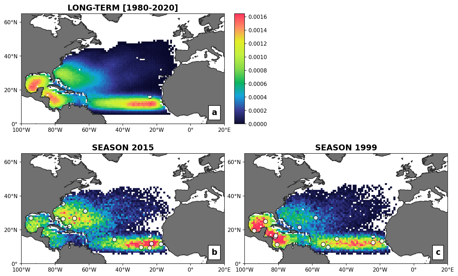
Figure 6 Spatial genesis density maps at 1° resolution; panel (a) shows smoothed-out static version of historical occurrences, while panels (b) and (c) illustrate the dynamic spatial probability of genesis accounting for SST and wind shear anomalies. The white dots show the historical cyclone genesis occurrence for the 2 years considered (2015 and 1999, see Fig. 7).

In a static TC risk model, the likely genesis location of a stochastic event is typically sampled from a probability density map representing a generalized version of historical records. An example of such a map is provided in Fig. 6a for the North Atlantic basin, where a spatial smoothing was applied to all 1980–2020 genesis coordinates (i.e., 2D convolution using a 5 × 3 spatial kernel). While this allows sampling from a climatology consistent with history, the approach does not account for season-to-season variability in climate conditions known to impact TC genesis likelihood. To condition the UTC genesis likelihood maps, we here adjust the static probabilities using a simple dimensionless scaling factor that is based on the ratio of SST and SHR anomalies for each grid cell k.

$$\begin{array}{}\text{(1)}& \mathrm{scaling}\left(k\right)={\displaystyle \frac{\mathrm{1}+{\mathrm{SST}}_{\mathrm{anomaly}}\left(k\right)/\left|\mathrm{SST}\right|}{\mathrm{1}+{\mathrm{SHR}}_{\mathrm{anomaly}}\left(k\right)/\left|\mathrm{SHR}\right|}}\end{array}$$

Physically, this adjustment ensures that the probability of genesis increases as the SST moves up from its climatological average and/or the vertical wind shear is reduced compared to its climatological state.

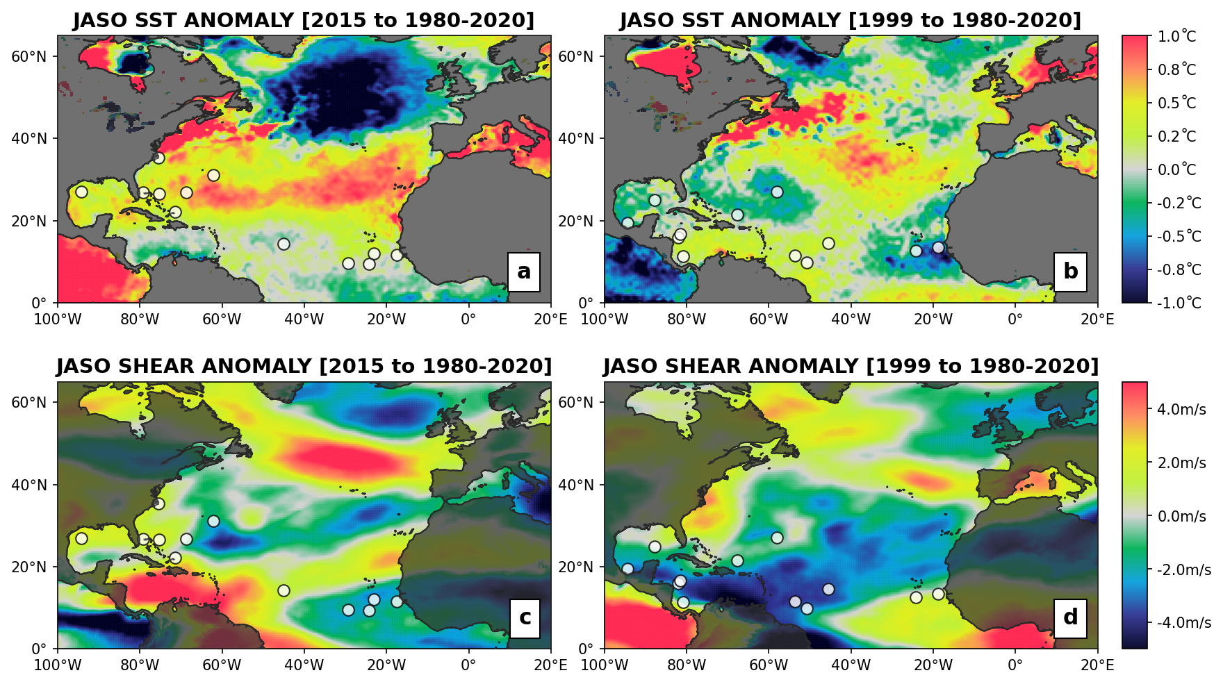
Figure 7 (a, b) SST and (c, d) SHR anomalies with regards to the 1980–2020 mean for July–October in (a, c) 2015 and (b, d) 1999. Historical TC genesis locations are shown in white.

Figure 6 provides an example of the adjusted genesis probability maps for two contrasting seasons: 2015 (Fig. 6b) and 1999 (Fig. 6c). In 2015, climate conditions show anomalously cold SSTs and strong wind shear conditions in the Caribbean Sea (Fig. 7a, c), while SSTs are anomalously warm in most of the mid-latitudes of the basin. This setup translates into an increased likelihood of genesis along the US East Coast and a reduction in the Caribbean Sea (Fig. 6b) when compared to the static historical baseline (Fig. 6a). Conversely, year 1999 is characterized by anomalously cold SSTs east of Florida and in the northwest Gulf of Mexico (Fig. 7b), with very favorable shear conditions across the Caribbean and southern Gulf of Mexico (Fig. 7d). The impact on the modeled genesis likelihood map is towards an increased probability in the Caribbean Sea/Gulf of Mexico and a reduction east of Florida. In both years, the patterns of actual observed event genesis (white circles, Fig. 6) are consistent with these regional trends in favorable environmental conditions.

As a way to quantify the added value of the dynamic scaling, we have also conducted the following evaluation exercise: for all 1980–2020 observed genesis occurrences, we compute the genesis probability under both the static model (P_static, Fig. 6a) and with the dynamic scaling of Eq. (1) (P_dyn). Over the full dataset of all 1980–2020 historical occurrences, the average climate-conditioned genesis probability P_dyn is increased by up to 14.8 % compared to the static version (P_static), i.e., from additional knowledge about the environmental setup, the dynamical model is statistically increasing genesis likelihood in regions where genesis has occurred. When we limit the evaluation to the North Atlantic data only, the increase in average genesis probability estimates is 28 %, likely thanks to better quality data records in the region. This simple analysis shows that the added climate information helps improve genesis likelihood estimates while also ensuring that the model reacts to physical changes that are known to influence TC formation.

Once the starting position of an event is known, a similar approach is used to allocate a starting date. The likelihood of genesis for a given month is computed as the average of two components:

• a probability density function fit to observed historical records (P_hist), and

• a probability density function derived from monthly gridded SST, SHR, and MSLP variables (P_clim).

Using historical genesis locations and associated climate conditions, three probability density functions (P_SST, P_SHR, P_MSLP) are first independently derived to link the likelihood of genesis in a month to different levels of monthly SST, SHR, and MSLP. These are then combined into P_clim as follows:

$$\begin{array}{}\text{(2)}& P_{\mathrm{clim}}=P_{\mathrm{SST}}\cdot P_{\mathrm{SHR}}^{\mathrm{2}}\cdot P_{\mathrm{MSLP}}.\end{array}$$

P_clim allows conversion of the gridded climate fields into a monthly time series of probability maps. From knowledge of the sampled genesis location (see above), a time series of monthly probability is extracted and averaged with the climatological probability (P_hist). After linear interpolation of the monthly probabilities to daily resolution, a genesis day is sampled. Finally, the hour of genesis is uniformly sampled within the chosen day, and the date gets incrementally updated with the storm hourly displacements.

2.2.4 Track trajectory

As is common for most TC risk modeling systems (Hall and Jewson, 2007; Bloemendaal et al., 2020; Arthur, 2021), our approach to modeling individual event trajectories is to simulate incremental changes in latitude (dlat in ° h⁻¹) and longitude (dlon in ° h⁻¹) at fixed time intervals (1 h in this study). Under that framework, a track trajectory is simulated by iteratively sampling the next displacement from distributions conditioned on parameters at current and past locations (i.e., a Markov chain Monte Carlo (MCMC) approach).

However, instead of relying purely on the track history to date and its location to predict the next dlat and dlon increment distributions, the UTC algorithms are also trained to account for local environmental conditions capturing the dominant steering flow. To do so, we have overlaid the ERA5 reanalysis dataset on top of all historical TC events as reported in IBTrACS and have trained a quantile regression forest algorithm (see Appendix A4) to approximate the dlat and dlon distributions, conditional on regional steering patterns. At any time step along the track, the algorithm takes the following quantities as input to condition the distributions: storm translational speed, track heading angle, incremental changes in latitude and longitude since the previous time step, meridional and zonal components of the steering flow, spatial gradients of wind shear, mean sea level pressure, and sea surface temperature. To ensure the algorithms generalize information globally rather than memorize local historical behaviors, no direct location information (lat and lon coordinates) is provided. Conditional on this information, a distribution of dlat and dlon is modeled at every time step, allowing sampling of the next hourly track displacement (see Sect. 2.3).

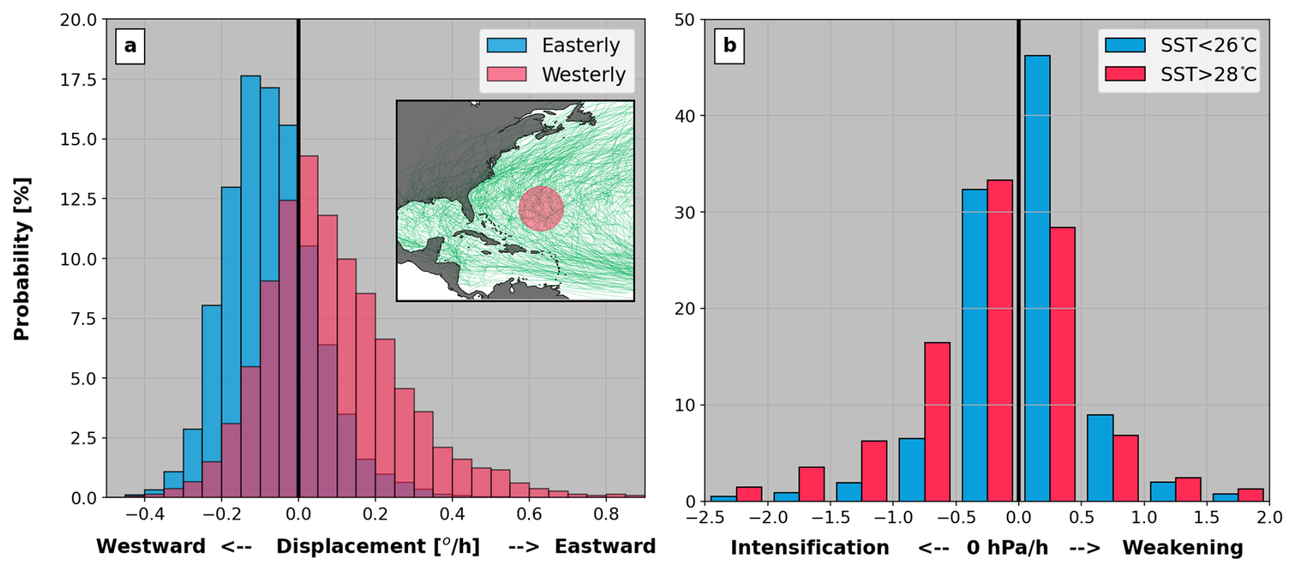
Figure 8 (a) Distributions of hourly change in longitude (dlon) simulated by the UTC for all events passing through the circle in the subpanel (for reference, IBTrACS data are displayed in green). Values of dlon corresponding to time steps with easterly (westerly) steering flow are shown by the blue (red) distribution. (b) Distributions of hourly change in center pressure (dCp) simulated by the UTC for the same region. Values of dCp corresponding to time steps with SSTs above 28 °C are shown in red, and those below 26 °C, in blue.

Figure 8a illustrates the role played by environmental conditions in simulating event trajectories in the UTC. Using a 20 000-year subset from the event set of Sect. 3.1, we extract the sampled dlon values of all events that pass through a selected region of the North Atlantic mid-latitudes (see map in Fig. 8a). Sampled dlon values that correspond to time steps when monthly steering winds are predominantly blowing east are shown as a red distribution, while the blue distribution represents time steps with steering winds blowing west. The ability of the UTC to react to dominant steering patterns is clear from the shift between both dlon distributions, with simulated tracks encountering easterlies (westerlies) more likely to move westward (eastward). Under that setup, strong anomalies in steering flow patterns are naturally reflected in the modeled event trajectories and therefore in the resulting statistics of landfall risk. It is this type of model behavior that allows translation of regional climate anomalies into shifts in TC landfall risk.

2.2.5 Event intensity

To simulate the intensity evolution over the lifetime of events, two separate algorithms are built. They target:

• the event intensity at the genesis point (center pressure, Cp_t=0, in mbar), and

• the increment change in intensity from one step to the next (dCp in mbar h⁻¹).

Both algorithms are trained in a similar fashion to the dlat and dlon models. By overlaying ERA5 data onto historical events as reported by IBTrACS, we can train quantile regression forest algorithms to approximate conditional distributions (see Appendix A4). In both cases, to condition the distribution, we use known storm parameters (Cp, previous pressure changes, and distance to land) and climate information (wind shear, mean sea level pressure, and sea surface temperatures, as well as their temporal gradients).

Figure 8b presents a similar exercise to Fig. 8a, where UTC modeled values of dCp for all events passing through the same domain. The distributions are split into cases with monthly SSTs above 28 °C (red) and below 26 °C (blue). The SST conditioning drives a clear shift towards a more likely intensification rate when ocean temperatures reach 28 °C. As a result, any important anomalies in SSTs are naturally reflected in the modeled UTC event intensities and allow intensification (resp. weakening) to occur over patches of anomalously warm (cold) water. By being closely connected to local environment conditions, the UTC intensity model is able to better capture the evolution of event severity as climate conditions evolve (e.g., see Sect. 3.2).

From a physical point of view, center pressure is the fundamental measure of storm intensity and is the logical starting point when modeling event intensification and weakening patterns. In terms of risk measurement, however, maximum winds offer a more relevant metric. It is the metric most often reported by media and used to categorize storms in the Saffir Simpson scale; it is also the basis for the estimation of TC-related damage. As a final step to the intensity module, we therefore translate our Cp estimates into maximum wind speeds (1 min sustained winds over water at 10 m, V_max). This is done following the methods published in Bruneau et al. (2024), where V_max is derived from the center pressure deficit via a coefficient α and α is modeled via a quantile regression forest model. The features consist of the center pressure at t and t−1, mean sea level pressure, and wind shear, as well as a water/land flag.

2.2.6 Lysis

Sections 2.2.4 and 2.2.5 describe iterative processes that terminate only when a lysis flag is triggered, typically corresponding to an important weakening of the system. Modeling the cyclone lysis is a difficult exercise due to the small amount of data available for training (a single lysis per historical cyclone, most often occurring over ocean). To construct a set of lysis likelihood targets that goes beyond the binary outcome of historical lysis occurrences, we first assign a probability of lysis to each time step of historical events (see Appendix A4). A random forest is then trained to predict this probability of lysis from knowledge of event properties, climate conditions, the time spent over land, and the topography setup. When generating events, the random forest algorithm is deployed to predict this probability at each time step. The probability is then used in a binomial draw to sample the survival/lysis outcome.

2.3 Model deployment steps

Having described how each of the UTC algorithms is developed, we now provide the detailed sequence of steps leading to the generation of UTC event sets:

1. Take monthly gridded data fields for climate state X (e.g., from a historical year of ERA5 reanalysis or alternative gridded climate dataset).

2. Extract W_FLD,i weight values for selected PC_FLD,i modes of climate state X. Compute associated climate connector values.

3. Model distributions of annual TC numbers by basin conditioned on these connector values for climate state X.

4. Initiate sampling of stochastic years under climate state X.

   For stochastic year 1 to N:

   • a.

     Using the modeled distribution from Sect. 2.2, sample a number of TC events to simulate for each basin that year.

   • b.

     In each basin, initiate a loop over all events.

     For event 1 to nTC:

     • i.

       Sample the genesis point from knowledge of the environment conditions in the basin (sea surface temperature and wind shear).

     • ii.

       Sample the genesis date based on the genesis location and environment conditions.

     • iii.

       Given the genesis location, date, and local environmental conditions, simulate the distribution of likely starting intensity (Cp in mbar). Sample the intensity value.

     • iv.

       From knowledge of the above and regional steering conditions, model the distribution of likely latitude and longitude displacements over the following hour. Sample the displacement values, and move the storm.

     • v.

       From knowledge of the above and regional climate conditions, model a distribution for the increment in intensity to expect. Sample the increment values, and update the storm intensity.

     • vi.

       Model a probability of lysis, and sample lysis occurrence with a binomial draw. If lysis occurs, stop and move to the next event; otherwise, repeat steps iv, v, and vi until lysis occurs.

     • vii.

       Model 1 min sustained winds over water (V_max) from Cp following Bruneau et al. (2024).

3 A probabilistic view of global tropical cyclone risk

In this section, we analyze global tropical cyclone risk, as modeled by the UTC under climates of the 1980–2023 period (i.e., the deployment period). The objective is 2-fold:

• UTC evaluation and risk analysis – Ensure that our historical experience over the 1980–2023 period is consistent with the probabilistic view simulated by the UTC (Sect. 3.1). For that purpose, the UTC is forced with ERA5 reanalysis data for 1980–2023. This dataset provides a view of the climate we have experienced over the post-satellite era period, where global TC observations are most reliable.

• Counter-factual analysis – Quantify the additional risk variability attributable to uncertainty in the climate experienced over the period (Sect. 3.2). Here, 1980–2023 climate simulations from the NCAR CESM large ensemble product (LENS2 – Rodgers et al., 2021) are used to force the UTC. We have selected the 50 smoothed biomass burning (SBMB) ensemble members to allow sampling of other climate states that could have likely occurred over the 1980–2023 period (i.e., dimension B in Sect. 2.1).

3.1 Analysis of global risk patterns and comparison to historical experience

For every year in the 1980–2023 ERA5 reanalysis dataset, we run 2500 samples (i.e., N = 2500 – see step 4 in Sect. 2.3) to generate 110 000 years of stochastic TC activity globally (44 climates with 2500 realizations of each). Historical observations over the 1980–2023 period are compared to the UTC probabilistic view of basin-wide activity (Sect. 3.1.1), spatial severity distribution (Sect. 3.1.2), and landfall return period risk (Sect. 3.1.3). It is important to note that historical records should only be seen as one sample from the distribution of potential risk over the period. The UTC, on the other hand, is designed to approximate the full distribution from which the records were sampled. The most important aspect of this evaluation exercise is therefore to show that the observed sample (i.e., our historical experience) falls within the UTC modeled distribution, with occurrence statistics that are consistent with the modeled view. There is, however, no expectation that the observed sample should fall at the center of the distribution for all aspects under evaluation.

We choose to analyze and evaluate the modeled 1 min sustained winds (V_max), as they represent a natural measure of TC impact. All IBTrACS results are shown using the “USA_WIND” data field from the HURDAT database (Landsea and Franklin, 2013) and the US Navy Joint Typhoon Warning Center (JTWC), as it is based on a globally consistent and well-documented methodology (Knapp and Kruk, 2010).

3.1.1 Global TC activity

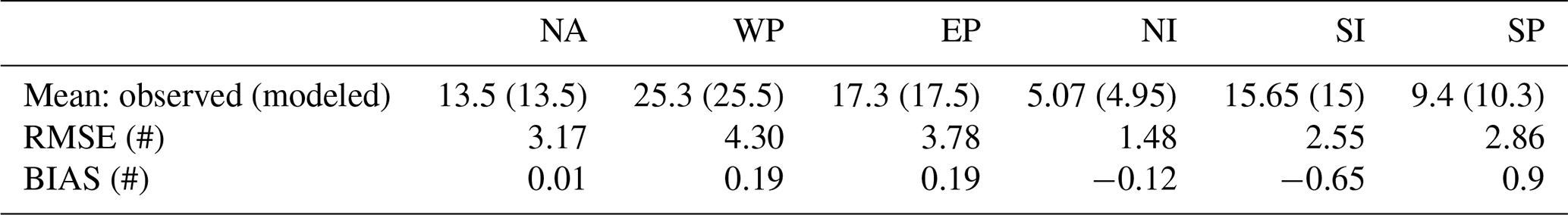
Figure 9 shows the density distribution of annual named storm numbers in the 110 000-year stochastic event set for each of the active basins and for each TC season of ERA5 forcing (1980–2023). They represent the likelihood of outcomes under each of the historical annual climate states (1st–99th percentile intervals are displayed in Fig. 9). Observed records are overlaid on all the distributions as white circles. They represent the one outcome that occurred under that observed climate state. As such, we should not expect to see the white circles at the center of the UTC distributions for all individual years; however, it is important that the circles do fall within the modeled distributions and that the overall statistics are in line with the UTC data. Over the full Fig. 9 dataset, observed occurrence levels are within the UTC 50th confidence interval in 64 % of cases, while 94 % fall within the 90 % confidence interval. Additional evaluation metrics are provided in Table 1.

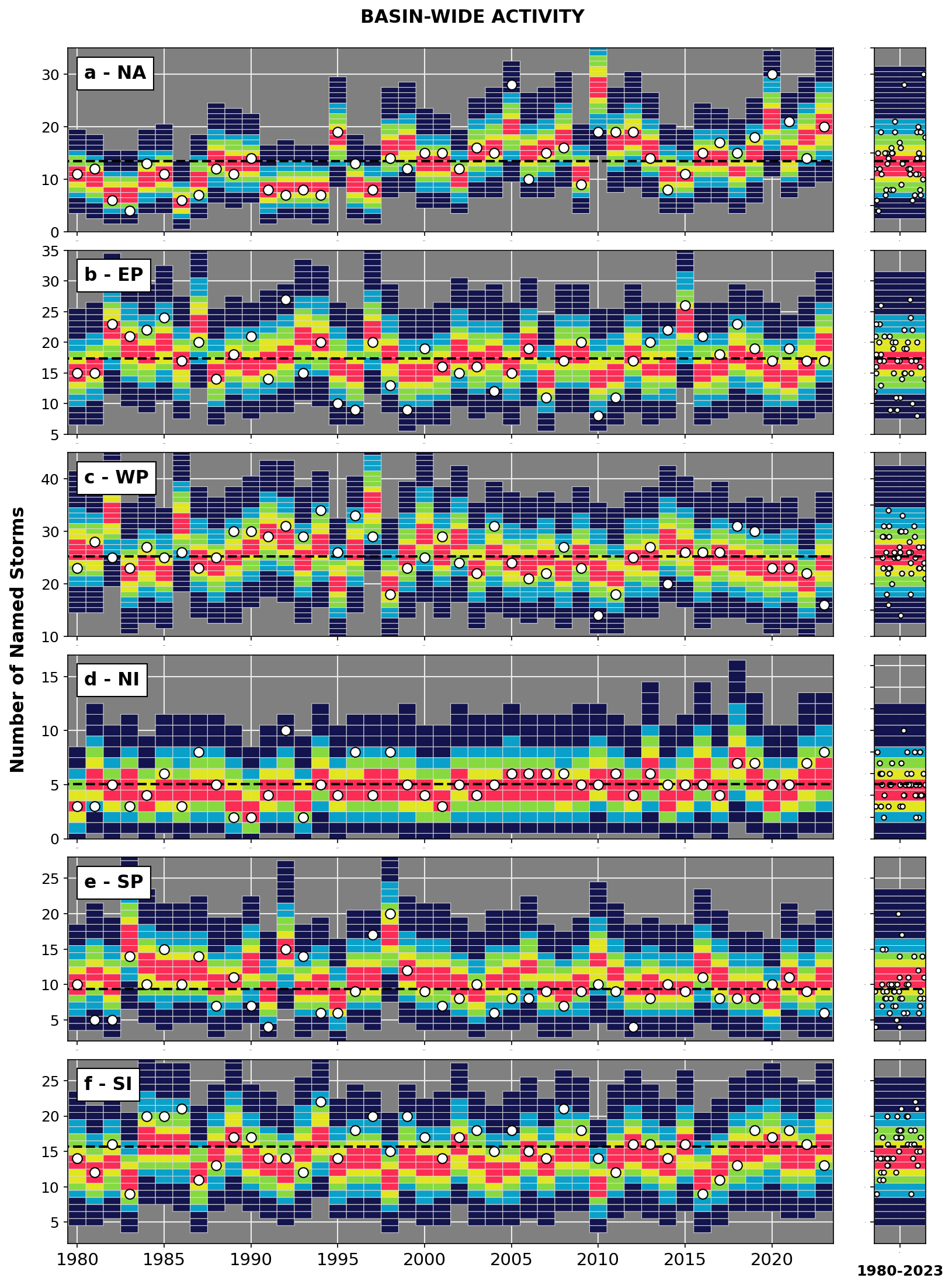
Figure 9 Distributions of named storm numbers from a 110 000-year UTC dataset forced by ERA5 reanalysis data of the 1980–2023 period for the (a) North Atlantic, (b) East Pacific, (c) western North Pacific, (d) North Indian, (e) South Pacific, and (f) South Indian basins. Historical occurrences from the Colorado State University database are shown as white dots, and UTC distributions averaged over the whole period (climatology) are shown in the right panels. The simulated 1st–99th, 10th–90th, 20th–80th, 30th–70th, and 40th–60th intervals are displayed.

Table 1 Statistical evaluation metrics for all six basins in the dataset from Fig. 9.

In all basins, the season-to-season variability in the modeled UTC distributions is consistent with variability in the observed TC numbers. This ability to capture season-to-season variability is only possible thanks to the climate-connected nature of the model. Without climate conditioning, every year would be assigned the same (static) activity distribution by basin (the average distribution over the period; see right panels in Fig. 9). This has important consequences when trying to assess short-term risk variability (e.g., the seasonal trends) as well as global connections in TC activity. For instance, by grouping the data from Fig. 9 in terms of climate regimes known to impact TC activity, we can quantify the shifts in basin-wide TC activity attributable to physical cycles such as ENSO and assess how activity levels in different basins are connected (e.g., anticorrelation between North Atlantic and East Pacific; Steptoe et al., 2017). Both of these aspects will be explored in separate studies where we illustrate the value of the UTC as a tool for seasonal risk forecasting, as well as for the quantification of global risk correlations.

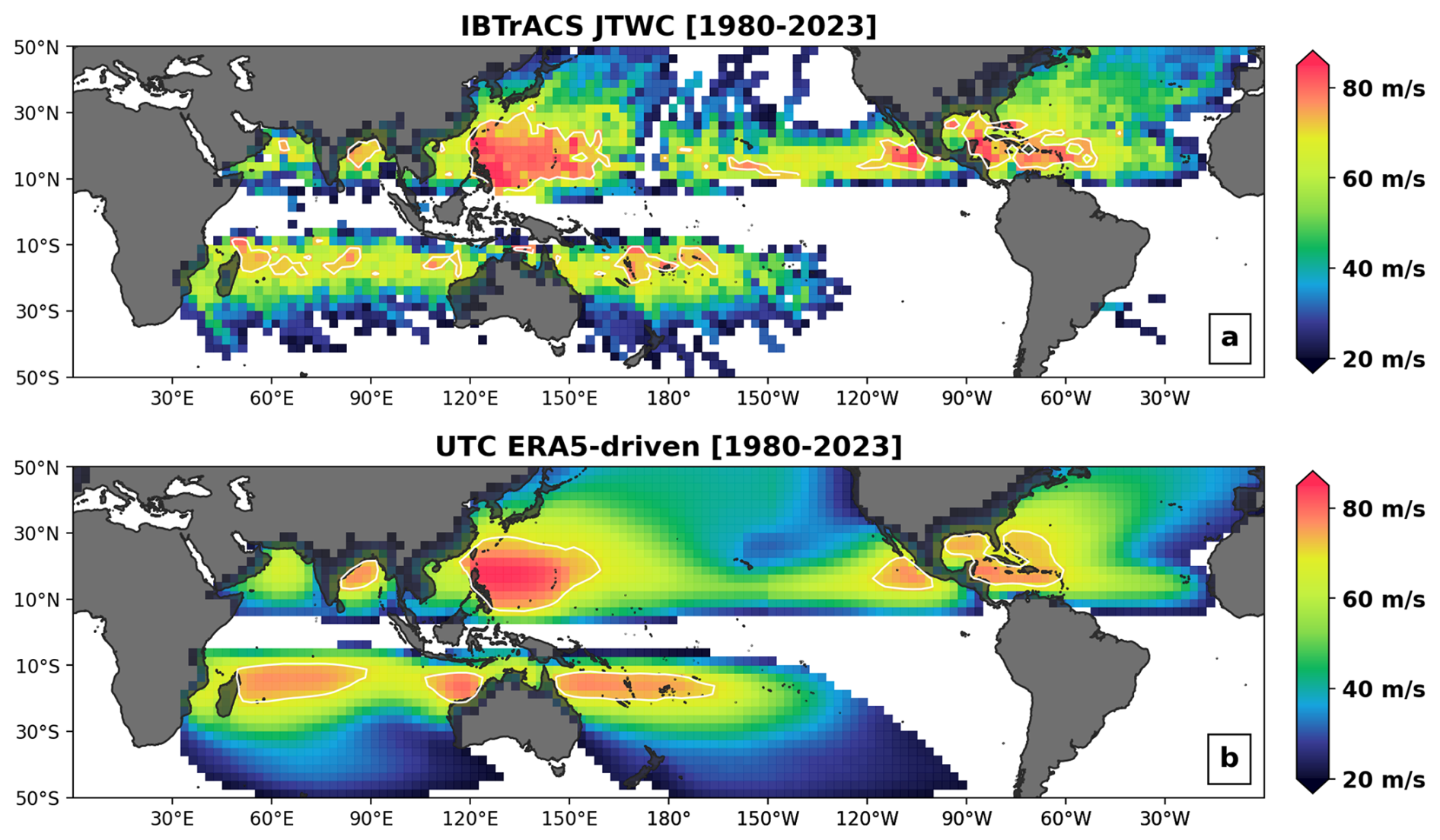
Figure 10 2.5° resolution map of (a) peak 1 min sustained winds recorded in IBTrACS over the 1980–2023 period and (b) expected 44-year peak sustained winds from the ERA5-driven UTC stochastic set (110 000 years of activity). The white contours represent the 70 m s⁻¹ wind level (Cat5 threshold).

3.1.2 TC spatial risk distribution across the globe

Beyond basin-wide activity numbers, one of the main goals of a TC stochastic event set is to capture spatial variability in risk severity within each basin. Observation records over the 44-year period of the post-satellite era are too scarce to provide a complete view of risk, but they do highlight regions where TC risk is concentrated. Analysis of maximum sustained TC winds globally over the 1980–2023 period (Fig. 10a) shows the eastern Philippines as the riskiest region on earth, followed by the western Caribbean. A closer look at the Gulf of Mexico or Florida regions reveals discontinuous patterns where important historical events are clearly identifiable among lower-risk neighboring levels. Such discontinuities in risk mapping are due to an insufficient number of seasons in the historical records to fully capture the spatial risk distribution of extreme events (the risk distribution is undersampled).

Using 110 000 years of simulations from the UTC, we can assemble a more consistent view of risk (Fig. 10b). The 110 000-year UTC event set is here split into 2500 groups of 44 years (i.e., 2500 iterations of the 1980–2023 period), allowing computation of 2500 equivalent versions of Fig. 10a. Figure 10b represents the grid cell average (2.5° resolution) of these 2500 versions and captures the expected peak winds over the 1980–2023 period for each grid cell. In other words, given what the UTC has learned from global historical records and the role played by climate physics in driving TC risk, peak winds of the magnitude reported in Fig. 10b should be expected when experiencing the climate of the 1980–2023 period. To gain some insight into the main drivers influencing the UTC view of risk, we also provide maps of peak season climatology (i.e., August–October in the Northern Hemisphere and December–February in the Southern Hemisphere) for the SST, SHR, U850, and V850 fields (Fig. 11).

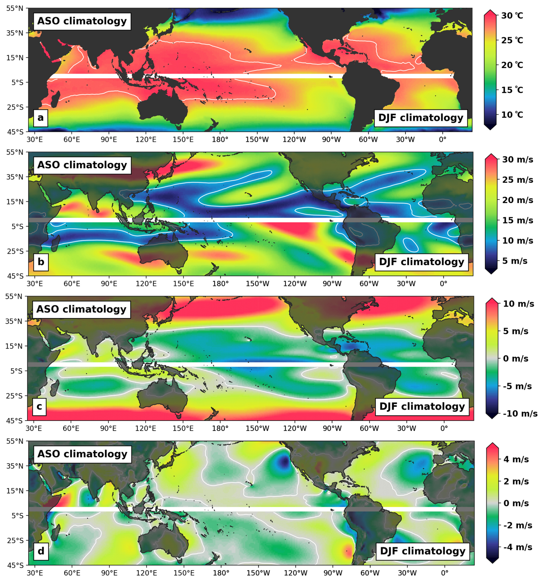
Figure 11 Peak season climatology (August–October in the Northern Hemisphere and December–February in the Southern Hemisphere for 1980–2023) for ocean surface temperatures (a), vertical wind shear (b), and meridional (c) and zonal (d) components of the 850 hPa winds. Contour lines correspond to 28 °C ocean temperatures (a), 10 m s⁻¹ wind shear (b), and the 0 m s⁻¹ steering (c, d).

For the North Atlantic (NA) basin, the regions of peak risk are very consistent with historical records. This is an important result, as the NA is the region of the world where we have access to the best quality of observation records over the 1980–2023 period. Category-5-level winds (i.e., 1 min sustained winds of 70 m s⁻¹ – the white contours in Fig. 10) are expected to occur during the period for regions along the Caribbean islands, Gulf of Mexico, and southern Florida (Fig. 10b). This is in line with historical records (Fig. 10a) and directly relatable to favorable peak season climatological conditions with warm SSTs (above 28 °C, Fig. 11a) and weak vertical wind shear (below 10 m s⁻¹, Fig. 11b). Patterns of cooling SSTs, higher vertical wind shear, and a strong westerly component of the steering flow (Fig. 11c) also clearly help in understanding the reduction in risk north of the Florida coast.

For the East Pacific (EP) basin, the regions of Category-5-level expected winds are again well aligned with historical evidence (Fig. 10) and coincide with favorable environmental conditions (Fig. 11) on the eastern side of the basin. Further west, a notable patch of large vertical wind shear is present over the Hawaiian Islands (Fig. 11b), along with a northerly component to the steering flow (Fig. 11c) that tends to protect the islands and translate into reduced risk levels both in terms of UTC expectations (Fig. 10b) and historical experience (Fig. 10a). More favorable conditions to the south of the islands allow for increased risk levels.

The western North Pacific (WNP) basin shows a good level of agreement between historical experience and UTC expectations. Environmental conditions in the basin are mostly favorable up to the Japanese coast, with very warm SSTs (Fig. 11a) and weak vertical shear (Fig. 11b). This translates into a wide region of peak risk to the east and north of the Philippines. As is the case on the eastern coast of the US, there is an important decrease in risk when moving north towards central Japan, with a sharp SST gradient, strong vertical wind shear, and dominant westerly steering flow.

TC activity patterns in the North Indian basin are consistent between model expectations and historical experience (Fig. 10), with higher risk localized in the northern part of the Bay of Bengal. The presence of high vertical wind shear to the south acts to dampen activity; however, we note that peak activity in the basin does not occur during the August–October period displayed in Fig. 11 and, as a result, modeled patterns are not further analyzed from a physical point of view.

The largest discrepancies between UTC expectations and observation records occur in the Southern Hemisphere (SH). In particular, the UTC has wider expectations of peak winds for the northeast (east of Townsville) and northwest of Australia (north of Port Hedland), as well as for most of the northern part of the South Indian (SI) ocean (Fig. 10b). Environmental conditions during peak SH season are mostly favorable in these three regions (Fig. 11), which helps explain why the UTC expected levels are high. With SSTs around the 28 °C level and wind shear conditions below the 10 m s⁻¹ threshold, these areas are comparable to the Caribbean and southern Gulf of Mexico regions. Consequently, UTC expectations in terms of peak winds are of similar magnitudes (i.e., at the category 5 level). While it is possible that the discrepancies could be attributable to a model bias (e.g., missing some local physics) or overgeneralization, it is also likely that events in these regions are underreported in IBTrACS. Coverage of TC events in the South Indian ocean, in particular, is likely not as thorough as in other basins. In the northeast and northwest regions of Australia, historical records are in line with the UTC expectations at the coast (see also Fig. 13) but differ further out at sea. Here again, it is possible that events have been underreported away from their direct landfall impacts (no immediate risk to the population). The alternative would be that events tend to reach their peaks only at the coast, and the physical reason for such behavior is missed by our modeling approach/resolution. Steering flow patterns (Fig. 11c, d) around Port Hedland are worth noting, as they help explain the concentration of risk observed historically over that section of the coast (see Fig. 13r). A corridor of strong northerly steering above warm SSTs and a weak shear environment lead to increased risk expectations.

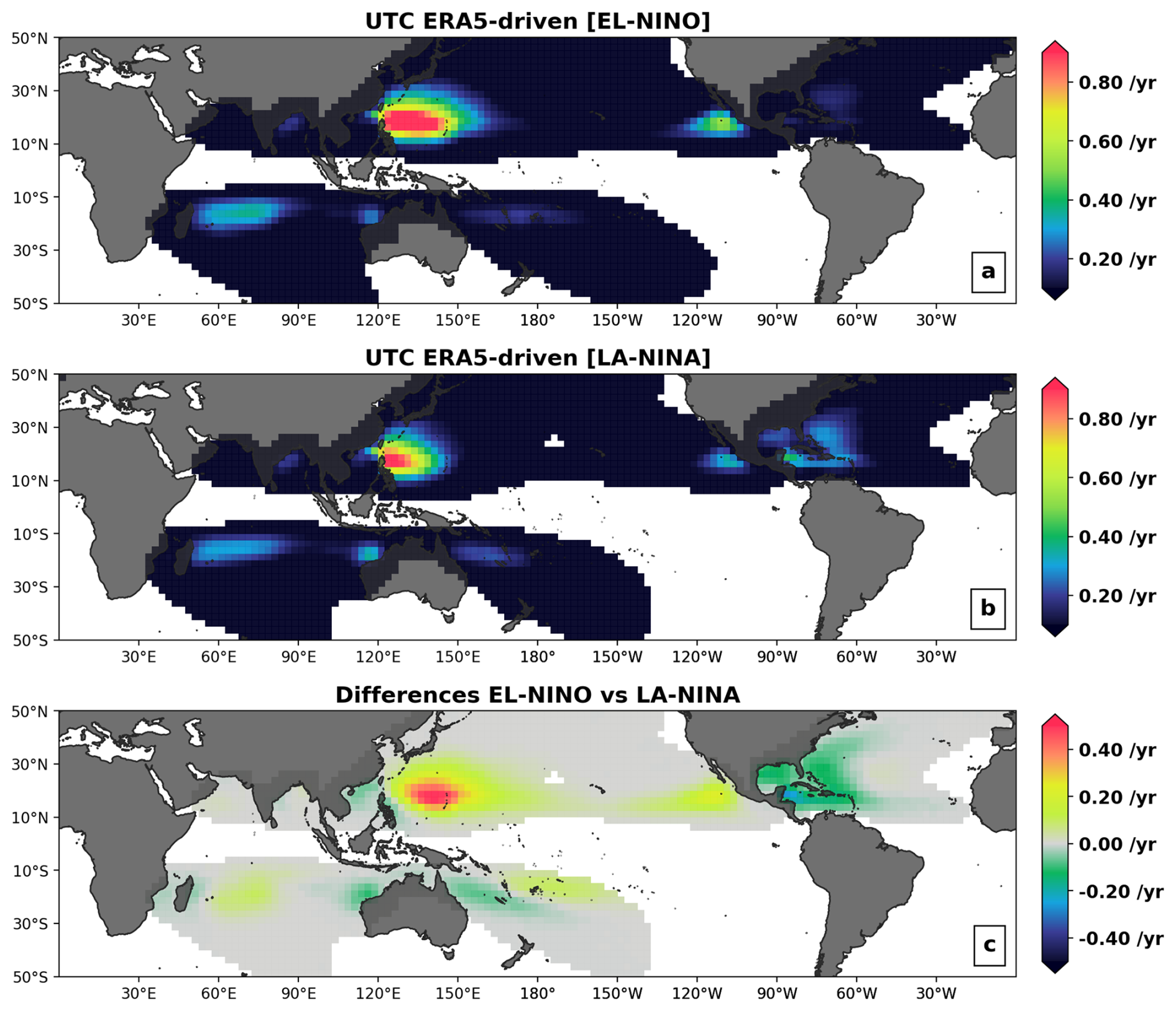
Figure 12 Annual occurrence rates of category 3 tropical cyclones for two subsets of the 110 000-year UTC event set, characterizing the 10 strongest El Niño (a) and La Niña (b) seasons in the period 1980–2023; each hemisphere uses the ENSO conditions of the in-season months (ASO for the Northern Hemisphere and DJF for the Southern Hemisphere). The absolute differences between El Niño and La Niña rates of Cat3+ are shown in the last panel (c).

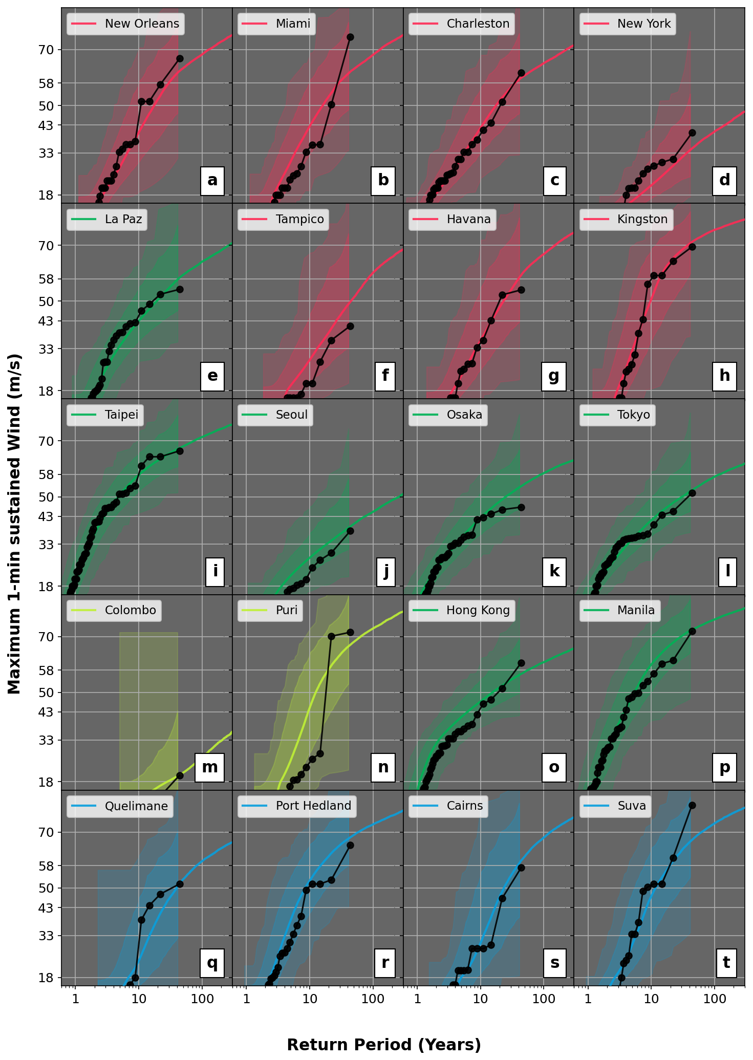
Figure 13 Return period of maximum 1 min sustained wind levels (m s⁻¹) in a 100 km circle centered on major coastal cities across the six active TC basins of the world. The thick, dark dotted line provides historical information for the period 1980–2023. The lighter shaded regions show the whole range simulated by the model considering 2500 samples of 44 years, while the darker shaded regions show the 5th–95th interval. Finally, the colored line illustrates the converged view, aggregating the 110 000 years of stochastic simulations.

The analysis of Figs. 10 and 11 shows that the UTC, driven by physical patterns known to be important to TC risk, is able to reproduce a global TC risk severity distribution that is consistent with historical records. As such, it provides a reliable tool to assess the impact of climate phases linked to shifts in patterns of ocean temperatures, vertical wind shear, or steering currents. As an example, we here briefly discuss the influence of the ENSO cycle. La Niña events are characterized by a western shift in warm ocean temperatures in the Pacific, with a resulting change in atmospheric circulation leading to reduced (increased) vertical wind shear in the Gulf of Mexico and Caribbean Sea regions (in the eastern Pacific). With these shifts in climate patterns directly conditioning the UTC event generation algorithms, the framework can be used to quantify the impact of the cycle on global TC risk. Here, we show the annual occurrence of category 3 events across the globe as modeled by the UTC for El Niño (Fig. 12a) and La Niña (Fig. 12b) conditions. The differences between both states is also shown in Fig. 12c. Consistent with the shifts in climate conditions described above, the risk of major hurricane occurrence in the Gulf of Mexico and Caribbean Sea under La Niña conditions is over 50 % higher than during El Niño conditions, with the opposite happening along the western Mexican coast. In the western Pacific, during El Niño conditions, the occurrence risk for category 3 events and above increases by up to 50 % on the eastern side of the basin, while the risk around the Philippines and the Chinese coast decreases. In the Southern Hemisphere, during La Niña conditions, category 3 occurrence risk increases around the Australian coast and decreases for the Pacific Islands.

3.1.3 TC landfall risk statistics

From the perspective of risk to society, the most relevant aspect to analyze is the severity distribution at landfall. We here focus on major metropolitan coastal regions across the globe and use the 110 000 years of UTC activity to assess return period wind speed levels at landfall (Fig. 13). For each region, the intensity of events is recorded for both the historical dataset and the UTC stochastic set. By ranking events in terms of their peak intensity in a 100 km circle centered on a given city (y axis, Fig. 13), we can then compute the associated return periods (x axis, Fig. 13).

For all panels, the 44 years of observations are reported as black dots, with the most intense events for each region located at the 44-year return period level. While graphically, this suggests a 44-year return period for these events, it is important to acknowledge how unreliable that estimate is. Quantifying the severity of rare extreme events from such a short record of observation years is an obvious issue, and here again the UTC offers an alternative by providing 110 000 years of activity. Return period intensity levels from the UTC are presented as solid-colored lines up to return periods of 1 in 300 years (i.e., beyond any available reliable historical records). Uncertainty bands are also reported by overlaying the regions covered by UTC subsets of 44 years (shaded areas). The darker shaded region captures the spread between the 5th and 95th percentiles from all 44-year subsets. The lighter shaded region extends to the entire dataset, showing the spread between the two most extreme 44-year subsets available in the 110 000-year simulation.

In all cases, the historical records fall within the range covered by the lighter shaded area, showing that our historical experience is contained within the distribution modeled by the UTC. The majority of data points are also contained in the range covered by the 5th to 95th quantiles, with the relative positions of the modeled averaged view (solid line) and historical records (dark line with dots) varying from one city to another. The modeled view sometimes suggests higher (e.g., Hong Kong SAR – Fig. 13o) or lower (e.g., New York – Fig. 13d) expected risk than experienced. As was the case for the discussion of Fig. 11, these discrepancies are mostly attributable to the limited length of historical records (undersampling of the risk) but could also be the result of local physical patterns being missed by the UTC modeling framework. The spatial resolution of the forcing climate data can, for instance, be too coarse to capture local steering shifts or sharp SST gradients in some regions (for example, around the Gulf Stream).

3.2 Impact of climate variability

The exercise presented in Sect. 3.1 focused on analyzing TC risk under the climate conditions observed between 1980 and 2023. Here, we expand the analysis to consider other climate conditions that could have occurred over the period (i.e., dimension B in Sect. 2.1). For this purpose, we ran an additional 550 000 years of stochastic TC activity based on the 50 smoothed biomass burning members of the CESM LENS2 (Rodgers et al., 2021) climate outputs for 1980–2023 (i.e., N = 250 samples, for 50 members, each covering the 44-year period). This allows reproduction of the analysis in Fig. 13, accounting for variability in the climate of the 1980–2023 period.

Unlike the ERA5 dataset, CESM LENS2 is not a reanalysis product. The data used in this study come from climate model runs without extensive assimilation of historical observations. While this is important to allow sampling of climate variability over the period, it also provides well-documented challenges in terms of model biases (Simpson et al., 2020; Lee et al., 2021).

To address this issue, we first compute a pixel-by-pixel and per-month climatology across all the members for each CESM climate variable from Sect. 2.1. We also compute and store a bias correction that aligns the data to the 1980–2020 ERA5 dataset. This bias correction is then applied to each member separately, ensuring that:

• on average, all the members are unbiased to ERA5 over the period 1980–2020, and

• the relative variability of each member is maintained after the correction is applied.

The stochastic event set used in this section is generated on this bias-corrected version of CESM LENS2, providing alternative climate TC risk consistent with what has been observed (ERA5) but through different paths.

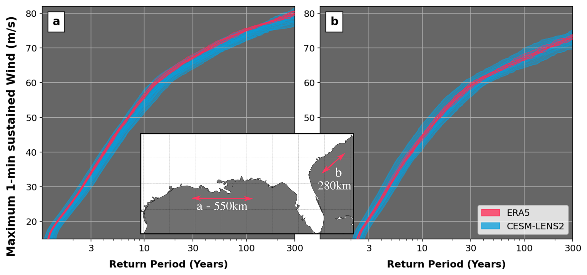
Figure 14 Return period of maximum 1 min sustained wind levels (m s⁻¹) along two segments of the US coast (inset) for 10 sets of an 11 000-year event set driven by ERA5 1980–2023 climate (red curves) and 50 sets of 11 000 years driven by the CESM LENS2 over the same period (blue curves).

Figure 14 below shows 60 curves capturing the return period risk for events crossing segments of the coast in Louisiana (Fig. 14a) and the Carolinas (Fig. 14b). The 50 blue lines correspond to the 50 CESM LENS2 members and are each built from 11 000 years of stochastic activity; they represent 50 different views of the climate over the 1980–2023 period. The 10 red lines are subsets of the ERA5 forced stochastic set (i.e., the one analyzed in Sect. 3a). They are also built from 11 000 years of activity but are all representative of the exact same climate over the 1980–2023 period (the one we experienced). By including additional climate conditions, the CESM-driven curves (blue) cover a wider spread than when only the ERA5 climate is considered (red curves).

This missing variability is important: while the narrow spread of the red curves provides the impression that the modeled view of risk has converged, it is important to acknowledge that it is only sampling dimension A. Therefore, it has converged under the assumption that the only climate we could have observed over the 1980–2023 period is the one portrayed by ERA5. When considering the alternative climates from CESM, the spread widens (blue curves). The UTC is now sampling a more complete risk distribution.

At the category 5 wind speed threshold of 70 m s⁻¹ for instance, the red curves all assign a return period between 40 and 45 years in Louisiana (Fig. 14a). The range covered by the blue curves, on the other hand, goes from 40 to 80 years, suggesting that the return period for Cat5 winds along that section of the coast could be much lower and that the climate experienced along the Louisiana coast may have been on the unlucky side with regards to its influence on hurricane risk. At the same threshold of 70 m s⁻¹ along the Carolina coast, the ERA5-driven view of risk is once again converged towards an estimate of 160–180 years. However, once we allow sampling from the wider range of climates covered by the CESM simulations, the estimates range from 100 to 300 years. Note that similar patterns can be observed at other intensity thresholds, with the width of the CESM spread narrowing for lower winds.

The ability to sample dimension B comes with a heavy computing cost (5x dimension A in the example above). Yet, the analysis of Fig. 14 shows that it has an important impact on our estimates of landfall risk distributions. The inclusion of that extra layer of risk variability is even more important when considering risk under future climate conditions, given the larger associated uncertainty. The use of the UTC to derive a forward-looking TC event set will be presented in a follow-up study, with two key use cases:

1. Deploy the UTC with seasonal climate projections (e.g., 51 members from the ECMWF monthly seasonal forecast). This allows generation of a seasonally conditioned TC stochastic event set, translating projected anomalies in SST, wind steering, and vertical wind shear patterns into regional shifts in TC risk for the season ahead.

2. Deploy the UTC with future climate projections (e.g., CESM members for the 2025–2100 period). This allows analysis of projected shifts in regional TC risk over the coming decades, under varying levels of global warming.

In both use cases above, the inclusion of dimension B is critical. Focusing on only one climate path vastly undersamples the full risk distribution, with important implications in terms of risk management and mitigation.

4 Conclusion

Stochastic event sets have made it possible to understand and manage tropical cyclone (TC) risk for over 3 decades. They are particularly useful in quantifying tail risk far beyond historical experience. However, to date, they have mostly been built from statistical relationships fit to historical records, without accounting for variability in the state of the climate. We here present an alternative approach (Unified Tropical Cyclone – UTC), where we explicitly connect the event generation algorithms to an input climate state. After an initial description of all algorithms involved in the climate-connected event generation process, we show results from two stochastic event sets representative of the 1980–2023 climate.

First, we force the UTC with reanalysis data over the period and compare the resulting view of risk to historical records. This analysis shows that the UTC modeled view is consistent with our historical experience over the past 44 years. It also highlights known limitations when it comes to assessing risk levels from historical records only: the period of reliable global records is too small, and, as a result, (i) it undersamples the spatial distribution of risk (Fig. 10) and (ii) misrepresents the likelihood of rare extreme events (i.e., tail risk, Fig. 12). Using 110 000 years of stochastic activity from the UTC helps in analyzing global TC risk beyond these limitations.

We then extend the analysis using additional forcing from a global climate model (CESM LENS2) over the same period to quantify the impact of climate variability. Accounting for this additional dimension of risk variability increases the sampling space (Fig. 14) and allows analysis of physically realistic scenarios that fall outside of the scope covered by traditional TC risk assessment frameworks. While we take measures to correct for model biases, a limitation of the current analysis is the use of a single model source (CESM). Future work will aim to include alternative model sources to expand the range of climate forcing considered.

The natural next step is to deploy the UTC under forward-looking climate scenarios, allowing risk assessment in the context of the season ahead or mitigation and planning strategies for the decades ahead. For such applications, the need to include sampling of climate variability (dimension B) is even more important, given the additional uncertainty associated with future climate projections and pathways.

Appendix A: Technical description of event generation algorithms

A1 Principal component analysis of gridded climate data

In machine learning terminology, principal component analysis (PCA) falls into the category of unsupervised learning algorithms. These are methods designed to identify patterns in large datasets without being told what to look for (the learning step does not involve any explicit target). Thanks to PCA, gridded fields can be decomposed into a series of patterns ranked in terms of how much data variability they explain. A typical use of PCA is then to select only a subset of all patterns (those that explain most of the variability) to reduce the dimension of the original dataset. The approach applied here differs slightly in that the subset of patterns is selected based on how those patterns correlate to TC activity in various basins of the world (e.g., see Fig. 4).

Prior to PCA, the raw gridded fields are standardized via a centering/scaling step, where the time average of each cell is removed (centering) before normalization by the cell standard deviation over the time dimension (scaling). For each climate field (i.e., FLD = SST, MSLP, U850, U250, V850, V250, or SHR – see Sect. 2.2), a PCA is then performed on the standardized array. This results in the projection of the gridded fields into a set of orthogonal vectors (principal components – PC_FLD,i – see Fig. 3) with associated coordinates, or weights (W_FLD,i).

For a given field (e.g., FLD = SST), the full decomposition of the raw monthly arrays can be formulated as follows:

$$\begin{array}{}\text{(A1)}& \mathrm{FLD}\left(t\right)={\mathrm{MU}}_{\mathrm{FLD}}+{\mathrm{SD}}_{\mathrm{FLD}}\times \sum _{i=\mathrm{1}}^{N_{\mathrm{pc}}}{W}_{\mathrm{FLD},i}\left(t\right){\mathrm{PC}}_{\mathrm{FLD},i},\end{array}$$

where MU_FLD is the time-averaged field array, SD_FLD is the standard deviation array, N_pc is the total number of principal components, and t is the time variable (monthly resolution). Note that the decomposition above can also be applied to stacked combinations of fields, where several arrays are layered. These will be referred to with a “+” sign in the following (e.g., FLD = SST + SHR + MSLP; see connector 3 in Appendix A2).

A2 List of climate connectors selected to condition TC activity

By computing the correlation between TC activity in each of the world's active basins and the W_FLD,i averaged over several months covering peak season activity, we can identify PC_FLD,i fields that are good candidates to connect climate state and TC occurrence (see Fig. 4). After screening these candidates to ensure that the physical reasons for the correlation are understood (see example in Sect. 2.2.1), we end up with a selection of 13 PC_FLD,i physical patterns to characterize a global climate state. The scalar values in Table A1 are referred to as climate connectors and are used to condition TC activity globally.

Table A1 List of connectors selected to condition the UTC model.

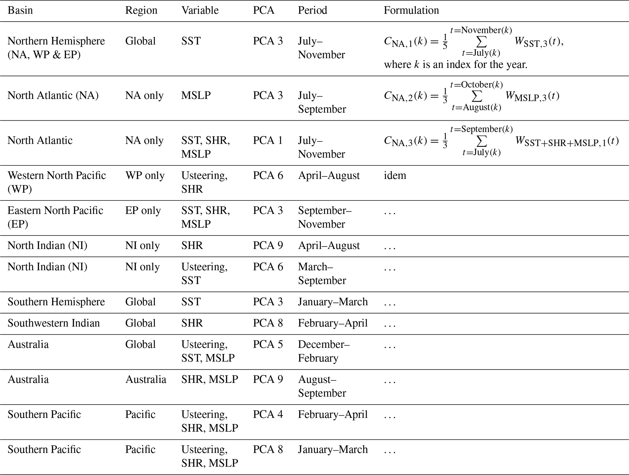
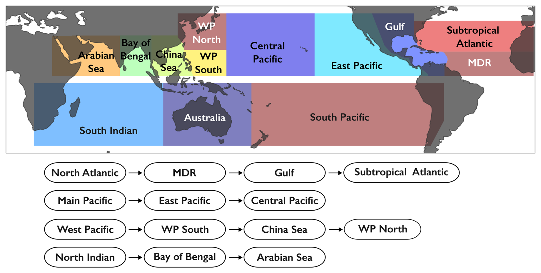
Figure A1 Sub-regions for tropical cyclone genesis, and chain of hierarchical Bayesian models.

To capture a realistic distribution of activity within the basins, we define broad sub-regions (Fig. A1). After initial sampling of the basin-wide activity, a series of hierarchical Bayesian models are used to approximate the contribution of each sub-region to the total activity number (i.e., ratio of total activity). To incorporate regional climate patterns of influence, several additional climate connectors are involved in the conditioning of the sub-region models (see example Fig. A2); these are listed in Table A2. The sampling chain of the hierarchical Bayesian model is also provided in Fig. A1.

Table A2 List of connectors selected to condition the UTC model for sub-region activity.

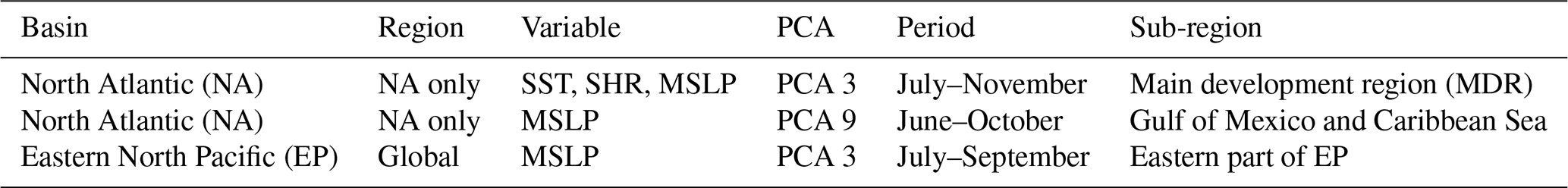
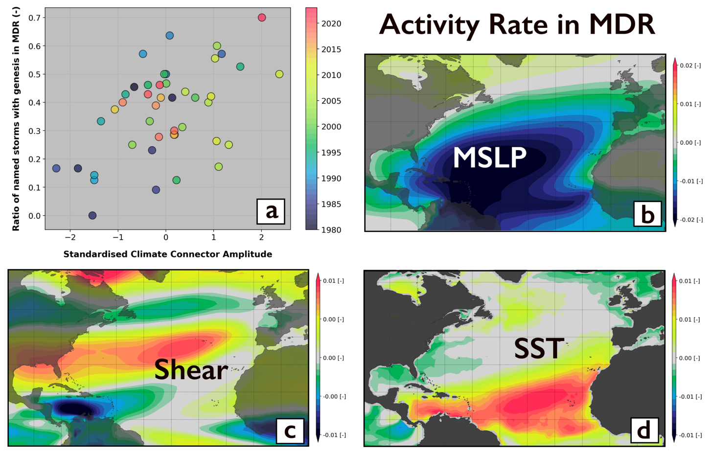
Figure A2 Example of climate connector used to condition the ratio of North Atlantic storms seeded in the MDR region. (a) Relationship between the climate connector chosen (see Table A2 – first row) and the rate in MDR. Panels (b), (c) and (d) show the mode of variability associated with this climate connector.

A3 Bayesian generalized linear model for TC annual frequency

Bayesian generalized linear models (GLMs) are commonly used to model conditional distributions when the training data are scarce (Elsner and Jagger, 2004). In this study, we use a Poisson GLM to model the conditional distribution of annual tropical cyclones in each basin. The λ rate from the Poisson distribution is conditioned on selected climate connectors (see Sect. A2). We use TC storm count data by season for the 1980–2020 period to train the relationship between λ and the climate state as described by the selected connector values.

As an example, the simplified model of Fig. 5 is presented below:

$$\begin{array}{}\text{(A2)}& \begin{array}{rl}& {\mathrm{nTC}}_k\sim \mathrm{Poisson}\left({\mathit{\lambda }}_k\right)\\ & \log \left({\mathit{\lambda }}_k\right)={\mathit{\beta }}_{\mathrm{0}}+{\mathit{\beta }}_{\mathrm{1}}{C}_{\mathrm{NA},\mathrm{1}}\left(k\right)\end{array},\end{array}$$

where k is an index for the season of interest and nTC_k represents the number of storms occurring in that year (season). A Poisson process is assumed, with λ_k referring to the rate for season k, and the logarithm of λ_k is modeled as a function of the July–November average W_SST,3 (i.e., connector 1 in Sect. A2 and the relationship shown in Fig. 4). The parameter vector $\mathit{\beta }=({\mathit{\beta }}_{\mathrm{0}},{\mathit{\beta }}_{\mathrm{1}})$ is specified by a multivariate normal distribution, as discussed in Elsner and Jagger (2004).

The complete model, as implemented in the UTC, involves three connectors for the North Atlantic basin:

$$\begin{array}{}\text{(A3)}& \begin{array}{rl}\log \left({\mathit{\lambda }}_k\right)=& {\mathit{\beta }}_{\mathrm{0}}+{\mathit{\beta }}_{\mathrm{1}}{C}_{\mathrm{NA},\mathrm{1}}\left(k\right)+{\mathit{\beta }}_{\mathrm{2}}{C}_{\mathrm{NA},\mathrm{2}}\left(k\right)\\ & +{\mathit{\beta }}_{\mathrm{3}}{C}_{\mathrm{NA},\mathrm{3}}\left(k\right).\end{array}\end{array}$$

Genesis models for all other active basins follow a similar structure, with the description of connectors involved in each model detailed in Table A1.

A4 Random forests and quantile regression forest algorithms

Supervised learning refers to the sub-group of ML algorithms that require an explicit target during the training phase. When trained with a large volume of data and carefully set up to avoid overfitting issues, these algorithms offer a very powerful tool to extract relationships without the need for a human to parameterize and tune their form. In this study, we rely mainly on a family of such algorithms called random forests because of their flexibility and robustness with regard to the overfitting issue.

The building block at the core of the random forest algorithm is the decision tree. Decision trees are essentially a series of nested if–then statements designed to recursively partition the training data into smaller groups that are more homogeneous with regards to the target. They are very popular due to their transparency and ease of interpretation. However, they are also known to lack stability, and small perturbations in the data can lead to very different tree architectures.

The random forest algorithm (Breiman, 2001) was developed to overcome these limitations by grouping together a large number of decision trees trained under slightly different conditions (random subsets of the input data and features at each tree node). The resulting ensemble of trees is then used as a cohort, and the prediction from the forest is obtained by averaging each tree's vote. This greatly reduces the challenges of overfitting and leads to a much more stable algorithm.

When used on new data to make a prediction, a random forest estimates the mean from the outcome distribution. In some cases, such as the example of Sect. 2.2.6, this is sufficient information. However, in other cases, it is desirable to retain information about the entire outcome distribution rather than simply focus on the mean prediction.

For such cases, we leverage an algorithm called quantile regression forest (Meinshausen, 2006), designed to keep the value of all observations in the terminal leaves to allow assessment of the full conditional distribution when making a prediction on new data. This contrasts with the standard random forest, where only the mean of observations in the leaves is kept (see Loridan et al., 2017, for more details).

In Sect. 2.2.6, we use a random forest algorithm to model lysis probability. To train the algorithm, we first assign a target lysis probability value to all historical TC track points in the IBTrACS database. Note that the target probabilities are capped at 0.5, acknowledging that some ambiguity can exist around the decision to stop reporting an event (i.e., the last point is not an exact representation of the time of lysis):

• Points for which a lysis occurred (last point recorded for a given event) are assigned a value of 0.5.

• Points within 24 h of lysis are assigned a value between 0 and 0.5 to reflect the belief that lysis was a likely possibility, following a simple linear law, i.e., $P_{\mathrm{lysis}}(t_{\mathrm{lysis}}-t)=\frac{\mathrm{1}}{\mathrm{2}t}$.

• All others points are assigned a value of 0.

We then train a random forest to predict this scalar value. Pressure field and pressure change to the previous time step, climate conditions (MSLP, SST, SHR, and their spatial gradient at the storm location), topography, time spent over land, and distance traveled over land are provided to the random forest algorithm to predict the probability of lysis.

Quantile regression forest (QRF) algorithms are the building block of our Markov chain Monte Carlo (MCMC) modeling of event trajectories and intensity evolution. We train the various QRFs involved to predict distributions of the hourly changes in latitude, longitude, and center pressure from knowledge of the event parameters at the current and previous step as well as the local environment (SST, vertical wind shear, and steering flow). The end result is a collection of QRF algorithms able to efficiently generate conditional distributions on the fly at every event time step knowing the state of the climate, therefore allowing sampling of all parameters needed to update the track to its next state (i.e., next center position and intensity).