Is considering (in)consistency between runs so useless for weather forecasting?

This paper addresses the issue of forecasting the weather using consecutive runs of one given numerical weather prediction (NWP) system. In the literature, considering how forecasts evolve from one run to another has never proven relevant to predicting the upcoming weather. That is why the usual approach to deal with this consists of blending all together the successive runs, which leads to the well-known “lagged” ensemble. However, some aspects of this approach are questionable, and if the relationship between changes in forecasts and predictability has so far been considered weak, this does not mean that the door is closed. In this paper, we intend to further explore this relationship by focusing on a particular aspect of ensemble prediction systems, the persistence of a given weather scenario over consecutive runs. The idea is that the more a phenomenon persists over successive runs, the more it is likely to occur, but its likelihood is not necessarily estimated as it should be by the latest run alone. Using the regional ensemble of Météo-France, AROME-EPS, and forecasting the probability of certain (warning) precipitation amounts being exceeded in 24 h, we have found that reliability, an important aspect of probabilistic forecasts, is highly sensitive to that persistence. The present study also shows that this dependence can be exploited to improve reliability for individual runs as well as lagged ensembles. From these results, some recommendations for forecasters are made, and the use of new predictors for statistical postprocessing based on consecutive runs is encouraged. The reason for such sensitivity is also discussed, leading to a new insight into weather forecasting using consecutive ensemble runs.

1 Introduction

Meteorological centres have improved their numerical weather prediction (NWP) systems over the past years, as summarized in Bauer et al. (2015). These improvements come in many forms and shapes, and some of them consist of major changes, increasing, for example, the model resolution (ECMWF with IFS in ECMWF, 2016, 2023; DWD with ICON in Deutscher Wetterdienst, 2022; and Météo-France with AROME-France in Brousseau et al., 2016), the ensemble size (Environment Canada with their global ensemble in Charron et al., 2010, and NCEP with GEFS in Zhou et al., 2022), or even the frequency with which forecasts are refreshed, i.e. the number of runs per day for a given model.

This last strategy is illustrated well by the Met Office, its regional ensemble MOGREPS-UK being run four times a day up to March 2019 and every hour since then (although fewer members are being produced in each run; see Porson et al., 2020). Moreover, its global ensemble, MOGREPS-G, has gone from two runs per day to four (Hagelin et al., 2017). Other centres have also adopted this strategy, such as Météo-France, whose AROME-France, the regional deterministic model that was initially run four times a day (Seity et al., 2011), has now been running every 3 h since July 2022. Likewise, AROME-EPS, its ensemble version, has been running four times a day since March 2018 compared to two times a day previously (Raynaud and Bouttier, 2017).

In our opinion, increasing the frequency of runs significantly affects how the weather is forecast. Along with the extension of the forecast range, it leads to the overlapping of consecutive runs in time so that nowadays, a given NWP forecast is usually considered by forecasters in combination with previous ones, especially if they are close in time. In this context, the variations from one run to another inevitably become important information to deal with, in particular for decision-making. However, this aspect of weather forecasting is relatively unexplored in the literature, as pointed out by Ehret (2010) or more recently by Richardson et al. (2020).

A review of the literature shows that most related studies have been concerned with quantifying run-to-run variability, underlining some features such as trends, convergence, consistency, or, on the contrary, “jumpiness”. Considering deterministic models as well as ensembles, several measures have been proposed and tested on various parameters, including geopotential height (Zsoter et al., 2009), sea level pressure (Hamill, 2003), temperature (Hamill, 2003; Zsoter et al., 2009; Griffiths et al., 2019), rainfall (Ehret, 2010; Griffiths et al., 2019), wind direction (Griffiths et al., 2021), large-scale flow over the European–Atlantic region (Richardson et al., 2020), or even tropical-cyclone tracks (Fowler et al., 2015; Richardson et al., 2024). To a lesser extent, the impact of run-to-run variability has also been studied from the point of view of decision-making. For instance, how the expense incurred by a given decision can be influenced by the way forecasts evolve over successive runs was investigated in McLay (2011). “Decide now or wait for the next forecast?” was the topic of Jewson et al. (2021), while communication challenges about forecast changes were explored in Jewson et al. (2022).

Although interesting, these studies tend to be rather limited when it comes to concretely predicting the weather using consecutive runs that may differ from each other. The decision-making studies partly address this issue but are conducted within a simplified theoretical framework that does not reflect the complexity of real-world decision-making (Jewson et al., 2021, 2022). On the other hand, most run-to-run variability measures have been introduced to identify features in the evolution of forecasts or to assess their consistency but never as additional information to improve weather forecasting. Actually, the relationship between changes in forecasts and the upcoming weather (that is, predictability) has rarely been studied as such, and only a few insights can be found sporadically (Persson and Strauss, 1995; Hamill, 2003; Zsoter et al., 2009; Ehret, 2010; Pappenberger et al., 2011; Richardson et al., 2020, 2024). It is suggested that forecast jumpiness is more a matter of modelling than predictability and that there is no strong correlation between run-to-run variability and forecast error. Consequently, the ECMWF forecast user guide advises forecasters not to rely on how a given NWP system behaves from one run to another (Owens and Hewson, 2018). The usual handling of successive runs is then quite straightforward: either consider the most recent one or blend them all together to create a “lagged” ensemble, as done, for example, by the Met Office within IMPROVER (Roberts et al., 2023). However, both approaches suffer from shortcomings, and further studies are needed to confirm the low usefulness of considering the evolution of forecasts for weather forecasting.

Only using the latest run can be a risky strategy because even if it is the most skilful on average, as forecast error increases with forecast range, it can sometimes be worse than the previous runs and can mislead forecasters. In particular, many high-impact case studies have cast doubt on this strategy by showing the importance of the previous runs: the catastrophic flood in Bavaria in August 2005 with GFS (Ehret, 2010), the torrential rainfall on 10 May 2006 over the southern United Kingdom with UK4 (Mittermaier, 2007), the flash flood during 15–16 June 2010 in the southeast of France with ARPEGE-EPS (Nuissier et al., 2012), and many more, even the recent Hurricane Laura in August 2020 and the ECMWF ensemble (Richardson et al., 2024).

Conversely, considering the sequence of successive runs is usually done by converting them into an ensemble, which is known as a lagged ensemble. If this approach can improve the forecast skill, in most studies it also assumes (Hoffman and Kalnay, 1983; Lu et al., 2007; Mittermaier, 2007; Ben Bouallègue et al., 2013) that all runs are equally likely, as the few attempts to weight runs have been unsuccessful (Ben Bouallègue et al., 2013; Raynaud et al., 2015). Therefore, the chronological order of runs is not accounted for, and no distinction is made between, for instance, a sequence of four deterministic runs with the two earliest forecasting light rainfall and the two latest forecasting intense rainfall and the opposite case. Yet this distinction seems crucial, at least from the forecasters' point of view. More generally, an ensemble composed of successive runs reflects, by definition, the response of a given NWP system to the recent changes in the atmosphere processed through its data assimilation algorithm. On the contrary, a standard Monte Carlo ensemble only reflects its sensitivity to many sources of uncertainty such as modelling approximations or initial conditions (Leutbecher and Palmer, 2008). These two ensembles do not carry the same information, and in this respect, distinguishing between a sequence of consecutive runs and a standard ensemble seems appropriate.

As it has been previously reported, this idea is somewhat at odds with the current state of the art since the evolution of forecasts has never been found to be strongly related to the upcoming weather. Nevertheless, we believe that further studies are needed to clarify that statement. Indeed, many results published in earlier work were based on run-to-run variability measures whose relevance may be questioned, as has been done, for instance, by Di Muzio et al. (2019) for the “jumpiness” index described in Zsoter et al. (2009). The same criticism can also be applied to the weather variables on which these studies are based. What has been found for the temperature or the geopotential height does not necessarily apply to other variables such as precipitation, which is characterized by a higher variability in both space and time (Ebert and McBride, 2000; Roberts, 2008). Finally, the run-to-run variability issue has mostly been addressed for low-impact weather (except in Richardson et al., 2020, 2024), while the relationship that might exist between changes in forecasts and predictability is often pointed out by forecasters during possible high-impact weather. Some related case studies have been documented and can be found in Kreitz et al. (2020), Caumont et al. (2021) (same event), or Plu et al. (2024).

For all these reasons, in this paper we intend to further explore the predictive skill of considering the (in)consistency between runs. This is done by focusing on a particular aspect of ensembles, the persistence of a given weather scenario over consecutive runs, and by investigating what that means in terms of predictability. Using the regional ensemble of Météo-France, AROME-EPS, and forecasting the probability of certain (warning) precipitation amounts being exceeded in 24 h, we study how the skill of the latest run or the standard lagged ensemble may vary depending on the persistence of the targeted events over the successive runs. From these results, recommendations for forecasters are made, as well as general thoughts on the usefulness of considering the evolution of forecasts for weather forecasting.

This paper is organized as follows. Section 2 introduces the dataset, Sect. 3 the methodology, and Sect. 4 the results that are discussed in Sect. 5 before the conclusion in Sect. 6.

2 Dataset

2.1 NWP system: AROME-EPS

AROME-EPS, the Météo-France high-resolution regional ensemble, is used in this study to assess the potential usefulness of considering run-to-run variability for weather forecasting. Having been run four times a day since March 2018, at 03:00, 09:00, 15:00, and 21:00 UTC, and making predictions of up to 51 h, AROME-EPS produces four forecasts every day coming from separate but close-in-time initializations that overlap at least until the end of the following day, which makes it well suited to this study.

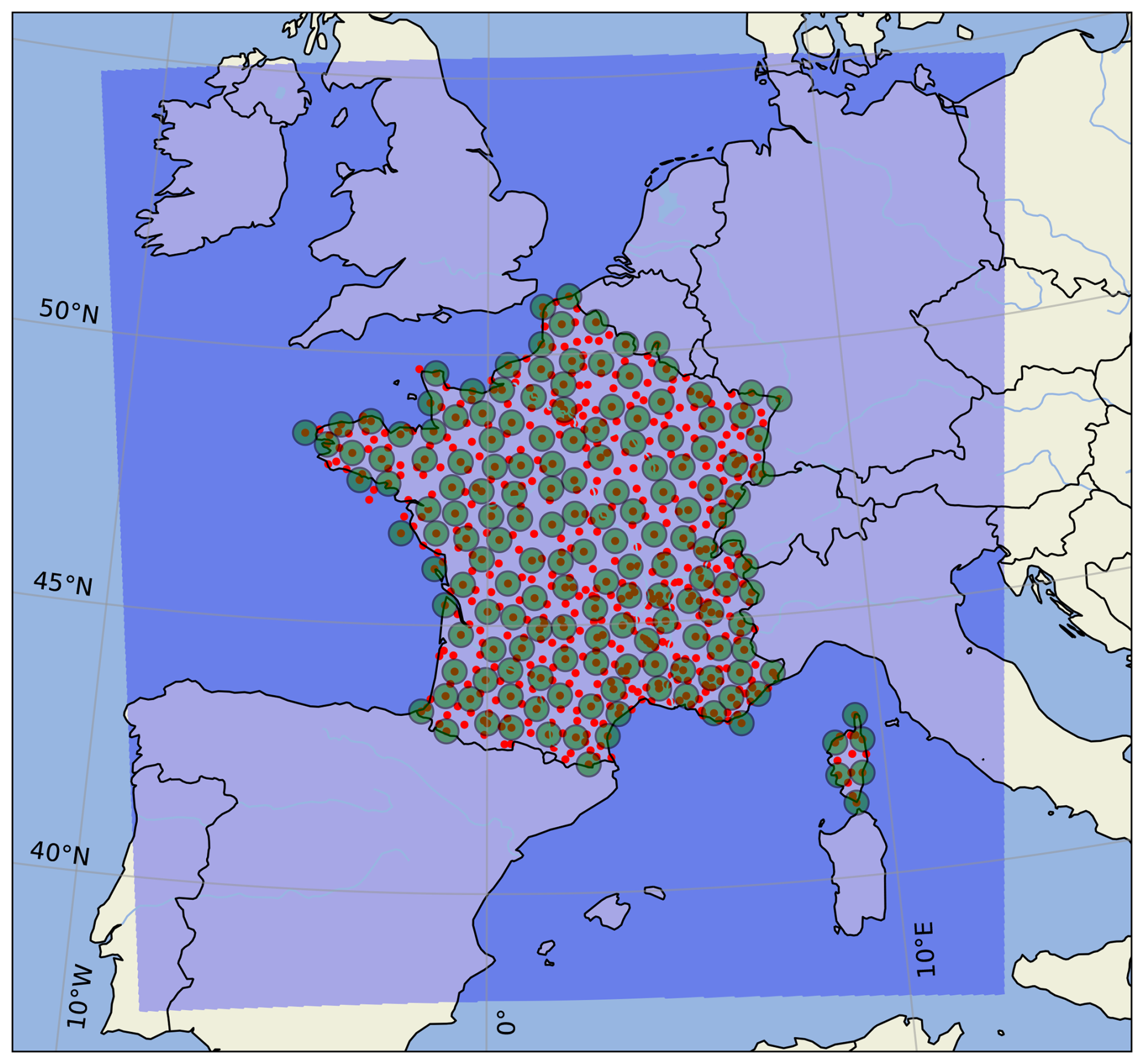
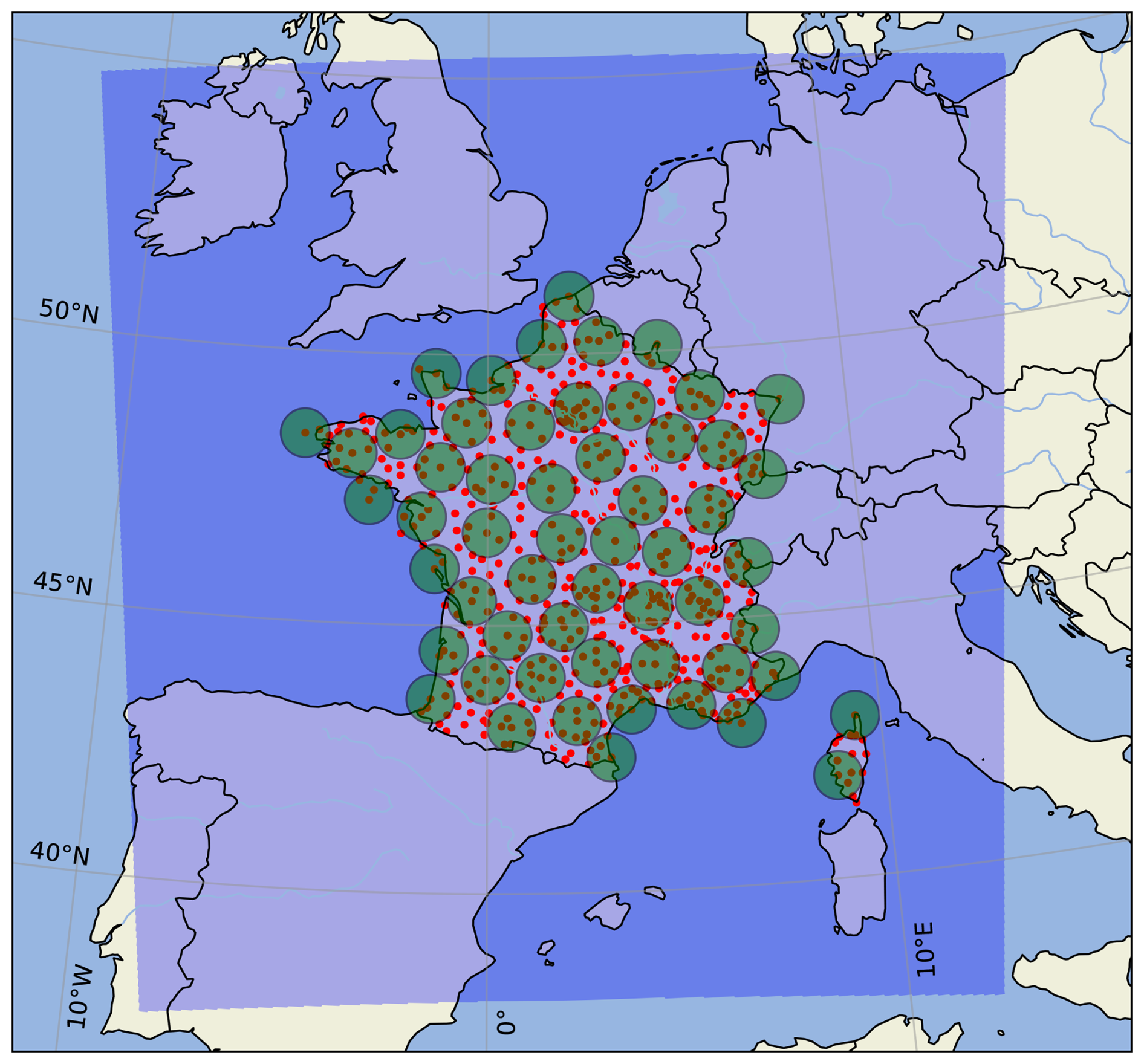
AROME-EPS comprises 17 members with a 1.3 km horizontal resolution and 90 vertical levels. One member is a control member, corresponding to AROME-France, the nonhydrostatic convection-permitting regional model of Météo-France (Seity et al., 2011; Brousseau et al., 2016). The other 16 perturbed members are obtained by sampling four sources of uncertainties: initial conditions (Raynaud and Bouttier, 2017), model errors (Bouttier et al., 2012), surface conditions (Bouttier et al., 2015), and lateral-boundary conditions (Bouttier and Raynaud, 2018). For practical reasons, AROME-EPS fields are extracted on a regular 0.025° × 0.025° latitude–longitude grid using a simple nearest-neighbour algorithm. The domain covered by AROME-EPS is displayed in Fig. 1.

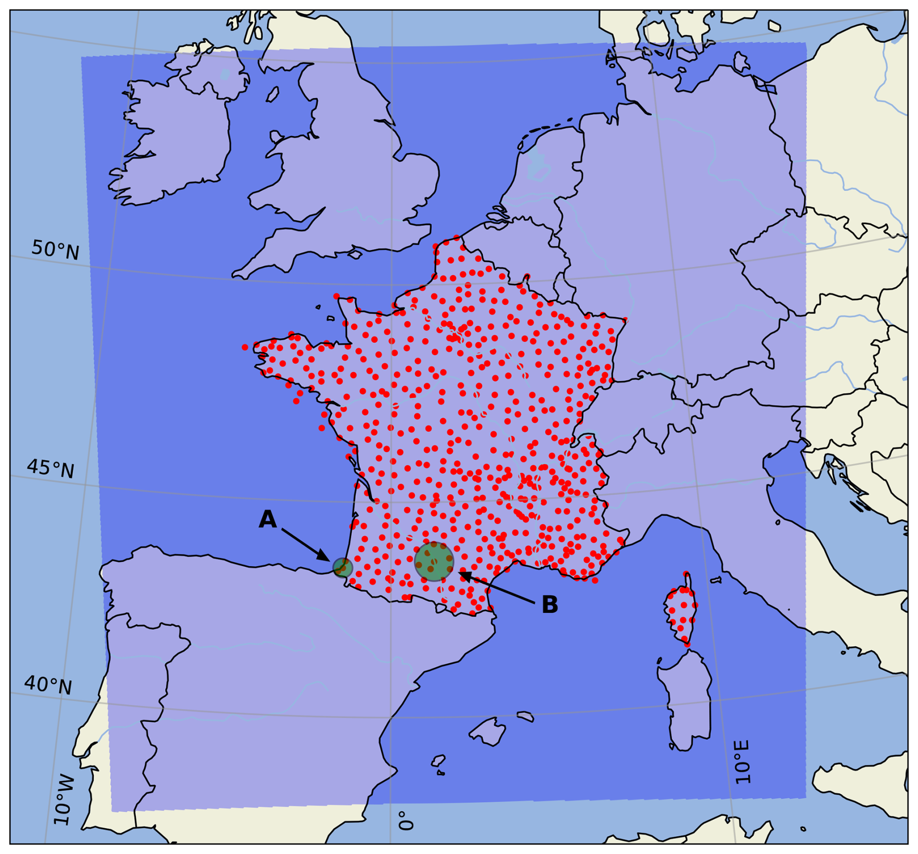
Figure 1 The AROME-EPS domain is shaded in blue. The RADOME rain gauges are represented by red dots. The green discs represent 25 and 50 km radius neighbourhoods in the vicinity of Biarritz (A) and Toulouse-Blagnac (B), respectively.

2.2 Parameter of interest: 24 h accumulated precipitation

This paper focuses exclusively on 24 h accumulated precipitation. As mentioned in the introduction, accumulated precipitation is characterized by large variability in both space and time (Anagnostou et al., 1999; Ben Bouallègue et al., 2020; Hewson and Pillosu, 2021), which makes this parameter challenging to predict and likely to show inconsistency between runs, as (once again) recently experienced by Météo-France forecasters during the Paris 2024 Olympic Games opening ceremony (Kreitz and Decalonne, 2025). The question of run-to-run variability has also rarely been explored in terms of accumulated precipitation: only Ehret (2010) and Griffiths et al. (2019) did it, dealing mostly with relatively light 3 or 6 h rainfall accumulation. The 24 h accumulation period is preferred over shorter periods, in particular because it summarizes the precipitation in a day without considering how the accumulation is distributed over the 24 h.

2.3 Observations and study period

The ANTILOPE quantitative precipitation estimate (QPE) algorithm (Champeaux et al., 2009) is used as the 24 h accumulated precipitation observations. ANTILOPE merges rain gauge data with radar reflectivity observations (Tabary, 2007), and provides data on a regular 0.025° × 0.025° latitude–longitude grid over a subdomain of AROME-EPS. Because ANTILOPE quality decreases with distance from radars and rain gauges, its use is restricted in this study to areas close to rain gauges from the RADOME network. RADOME is the real-time meteorological observation network of Météo-France (Tardieu and Leroy, 2003) and comprises 596 stations that are included by design within the ANTILOPE analysis. Figure 1 shows the RADOME coverage over mainland France. How AROME-EPS forecasts will be compared to these observations and how ANTILOPE will be precisely used in this study will be detailed in the Methodology section.

Finally, the study period over which the results are obtained runs from early July 2022 to late June 2023, approximately 1 year of data. 21 August 2022 has been removed due to missing AROME-EPS data.

3 Methodology

3.1 Use of the four daily AROME-EPS runs

This study focuses on daily precipitation, i.e. accumulated between 00:00 and 00:00 UTC the next day. To predict the daily precipitation on a given day, the four AROME-EPS runs of the day before are considered, with the 21:00 UTC run being the latest one and the 03:00 UTC run the oldest one, as depicted in Fig. 2. Note that hereafter, “Z21” stands for the 21:00 UTC run, “Z03” for the 03:00 UTC run, and so on. Each run is used to predict the probability of occurrence of targeted events corresponding to precipitation exceeding various thresholds during the following day. Such probabilities are computed using the frequentist approach, which consists of counting the number of members that have simulated the exceedance and dividing it by the total number of members (17), assuming that they are equally likely.

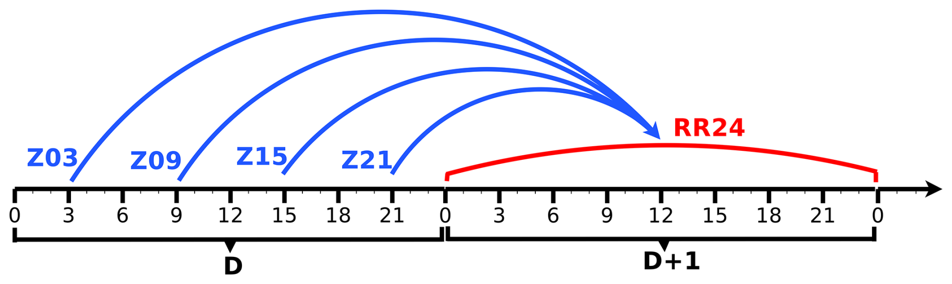
Figure 2 How the four daily AROME-EPS runs are used to forecast the 24 h accumulated precipitation (“RR24”) of the following day.

3.2 The risk persistence and its diagnostic

The purpose of this study is to further explore the predictive skill of considering (in)consistency between runs. Following discussions with Météo-France's forecasters, we chose to focus on a particular aspect of ensembles: the persistence of a given weather scenario over consecutive runs. The idea is that the more a scenario persists over successive runs, the more it is likely to occur, but its likelihood is not necessarily estimated as it should be by the latest run alone. Here, the latest run is Z21, and the event for which probability is computed is daily precipitation exceeding a given threshold. In this respect, the variable “risk_persistence” is defined as the number of previous runs that predict a nonzero probability of occurrence, i.e that have at least one member simulating the exceedance. Hence, if by “risk” we mean “nonzero probability of occurrence”, “risk_persistence” is equal to

$$\begin{array}{}\text{(1)}& \left\{\begin{array}{ll}\mathrm{0}& \text{if none of Z03, Z09 and Z15 had predicted}\\ & \text{a risk}\\ \mathrm{1}& \text{if only one run among Z03, Z09 and Z15}\\ & \text{had predicted a risk}\\ \mathrm{2}& \text{if only two runs among Z03, Z09 and Z15}\\ & \text{had predicted a risk}\\ \mathrm{3}& \text{if Z03, Z09 and Z15 had all predicted a risk}\end{array}\right..\end{array}$$

The usefulness of risk persistence is assessed in two different but complementary ways that are presented below. The relevance of its definition will be discussed after the results.

3.3 Manual assessment of the risk persistence usefulness

The first part of the results will be a study of how the Z21 skill varies according to the different modalities of risk_persistence. In order to establish a link with forecasters' impressions of the risk persistence, the reliability of the Z21 probabilities is assessed. Indeed, reliability measures by definition the agreement between forecast probabilities and the relative observed frequency of the target event (Toth et al., 2003). In practice, it amounts to investigating how Z21 may under/overestimate the probability of exceedance depending on whether or not the previous runs also predicted a nonzero probability. By doing this for various precipitation thresholds ranging from 0.2 to 100 mm, the dependence of the Z21 reliability on what the previous runs predicted can be highlighted.

3.4 Forecast calibration using the risk persistence information

The second part of the results will consist of “automatically” assessing the usefulness of risk persistence using a simple machine learning algorithm. The logistic regression is chosen since it has been widely used for precipitation (Ben Bouallègue, 2013, and references therein). If $P\left(t\right)=P(\text{RR24}⩾t)$ denotes the probability that daily precipitation exceeds t mm, then the logistic regression derives probabilities through the following equation:

$$\begin{array}{}\text{(2)}& P\left(t\right)={\displaystyle \frac{e^{z\left(t\right)}}{\mathrm{1}+e^{z\left(t\right)}}},\end{array}$$

where e^x = exp (x) is the exponential function, and z(t) is a linear function of N predictors X,

$$\begin{array}{}\text{(3)}& z\left(t\right)={\mathit{\beta }}_{\mathrm{0}}\left(t\right)+\sum _{i=\mathrm{1}}^N{\mathit{\beta }}_i\left(t\right)X_i\left(t\right).\end{array}$$

β₀ is the regression intercept, whereas β_i is the regression coefficient corresponding to the predictor X_i. The only predictors that are considered in this study are raw probabilities, for example from Z21, and risk_persistence is seen as a categorical variable. The potential added value of taking into account the risk persistence information is assessed by testing several regressions that differ only in the input predictors, mainly in the use or nonuse of risk_persistence. Those regressions are compared with each other and with the raw probabilities from Z21 and from the lagged ensemble based on the four daily runs (Z03, Z09, Z15, Z21). The regression coefficients that have been estimated for each modality of risk_persistence are also interpreted.

3.5 Spatial neighbourhood postprocessing

High-resolution models such as AROME-EPS are subject to the double-penalty effect, i.e. the fact that models that predict a “good” feature that is offset from the observation are penalized twice, with a false alarm and with a non-detection (Ebert, 2008). In order to cope with it, a 25 km radius neighbourhood is introduced. In concrete terms, the four AROME-EPS runs are used to predict the probability of daily precipitation exceeding a given threshold anywhere within a 25 km radius of the RADOME stations rather than predicting it precisely at station locations. This is done using the same upscaling procedure as in Ben Bouallègue and Theis (2013); i.e. the probabilities are generated from the maximum of each member within the area of interest. Observations are also upscaled, taking the maximum of the ANTILOPE QPE algorithm within the area, which includes RADOME stations by design. Other neighbourhood approaches could be used (some can be found in Schwartz and Sobash, 2017), but the upscaling procedure was preferred because of its relevance to the issuance of warnings (Ben Bouallègue and Theis, 2013).

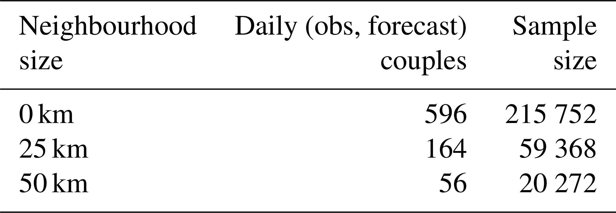
As many RADOME stations are less than 50 km apart, many verification areas will overlap if this neighbourhood method is applied to all stations. This is problematic since it can bias the score estimation and may lead to overfitting (Hastie et al., 2009). To avoid this, only RADOME stations that guarantee nonoverlapping verification areas are selected, and from the 596 initial stations, only 164 are finally used (see Fig. A1 in Appendix A). As shown in Table 1, the number of daily (obs, forecast) couples is thus substantially reduced, leading to a total of 59 368 over the 362 d of the study period. The upscaling procedure has, however, the substantial advantage of considering many more (and potentially interesting) precipitation values compared to only those observed at the rain gauge locations or predicted at specific grid points. In the following, all results are based on a 25 km radius neighbourhood unless explicitly stated otherwise. Their sensitivity to the spatial neighbourhood size and the relevance of the 25 km radius will be studied in a dedicated subsection and discussed later.

Table 1 Number of daily (obs, forecast) couples and the resulting sample size of the whole study period for each neighbourhood size.

3.6 Score and regression coefficient estimation

Reliability diagrams are used to assess the reliability of forecast probabilities. Here, they are obtained by plotting the relative observed frequency of the exceedance within the following 10 forecast probabilities bins: 0 %–10 %, 10 %–20 %, etc., with the upper bound of each bin excluded, except for the last bin. The statistical significance of the results (including these diagrams) is estimated by a bootstrapping procedure that produces 1000 resampled study periods of the same length. The bootstrap mean and Q5–Q95 confidence interval are shown but only for results whose estimation is sensitive to the sample used.

To complete the methodology, we would like to point out that unlike in Ben Bouallègue (2013), there is no unification term in the logistic regression: each exceedance threshold requires a specific estimation of the regression coefficients, which explains why the different elements of Eqs. (2) and (3) depend on t. Regression coefficients are estimated using a 1 d cross-validation procedure with a 5 d block separation between the test and training samples. In other words, 1 d of the study period is selected as a test sample, and the regression training is done over all the other days, excluding the 5 d on either side of the test day to ensure complete separation between the test and training samples. At the end of the cross-validation procedure, each day of the study period has been used once as a test sample. For further details on logistic regression, refer to Ben Bouallègue (2013) or Wilks (2011).

4 Results

4.1 Manual assessment of the risk persistence usefulness

In what follows, we take the perspective of a forecaster confronting the latest AROME-EPS run predicting a risk of a given precipitation threshold being exceeded in 24 h; i.e. at least one member of Z21 is predicting the exceedance. Then, in this context, the objective is to highlight the extent to which the forecaster has to take that latest run at face value, depending on whether or not the previous runs also predicted a risk of exceedance. For the sake of clarity, the two “extreme” scenarios of risk persistence are considered: the risk of exceedance is either “brand-new” (i.e. risk_persistence = 0) or “long-lived” (i.e. risk_persistence = 3). To begin with, the frequency of both cases is shown in Fig. 3. Firstly, it appears that the higher the precipitation amount (x axis), the rarer the risk_persistence = 3 case (blue line) and the more frequent the risk_persistence = 0 case (red line). In other words, exceedance scenarios involving large amounts of precipitation are less likely to persist over consecutive runs, and conversely, those involving smaller amounts tend to be more consistently predicted. Moreover, the more we focus on heavy rainfall, the more likely both cases are to occur, making these thresholds particularly relevant to the question of whether a forecaster should act differently in these two cases, as discussed below.

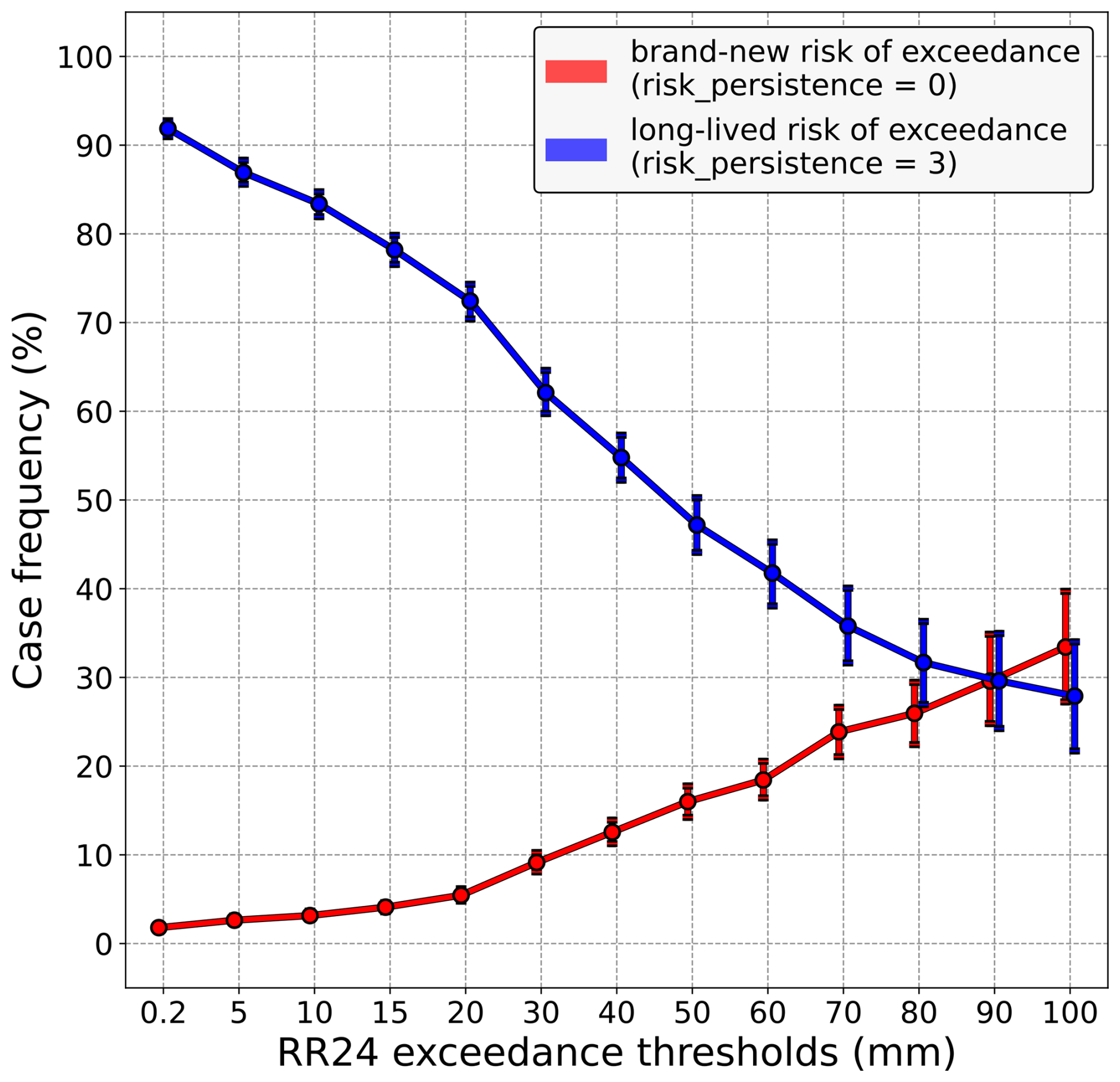
Figure 3 Frequency of “brand-new” risks of exceedance cases (red line) compared to frequency of “long-lived” risks of exceedance cases (blue line), conditioned on the precipitation amount (x axis). Vertical bars indicate 5 %–95 % confidence intervals.

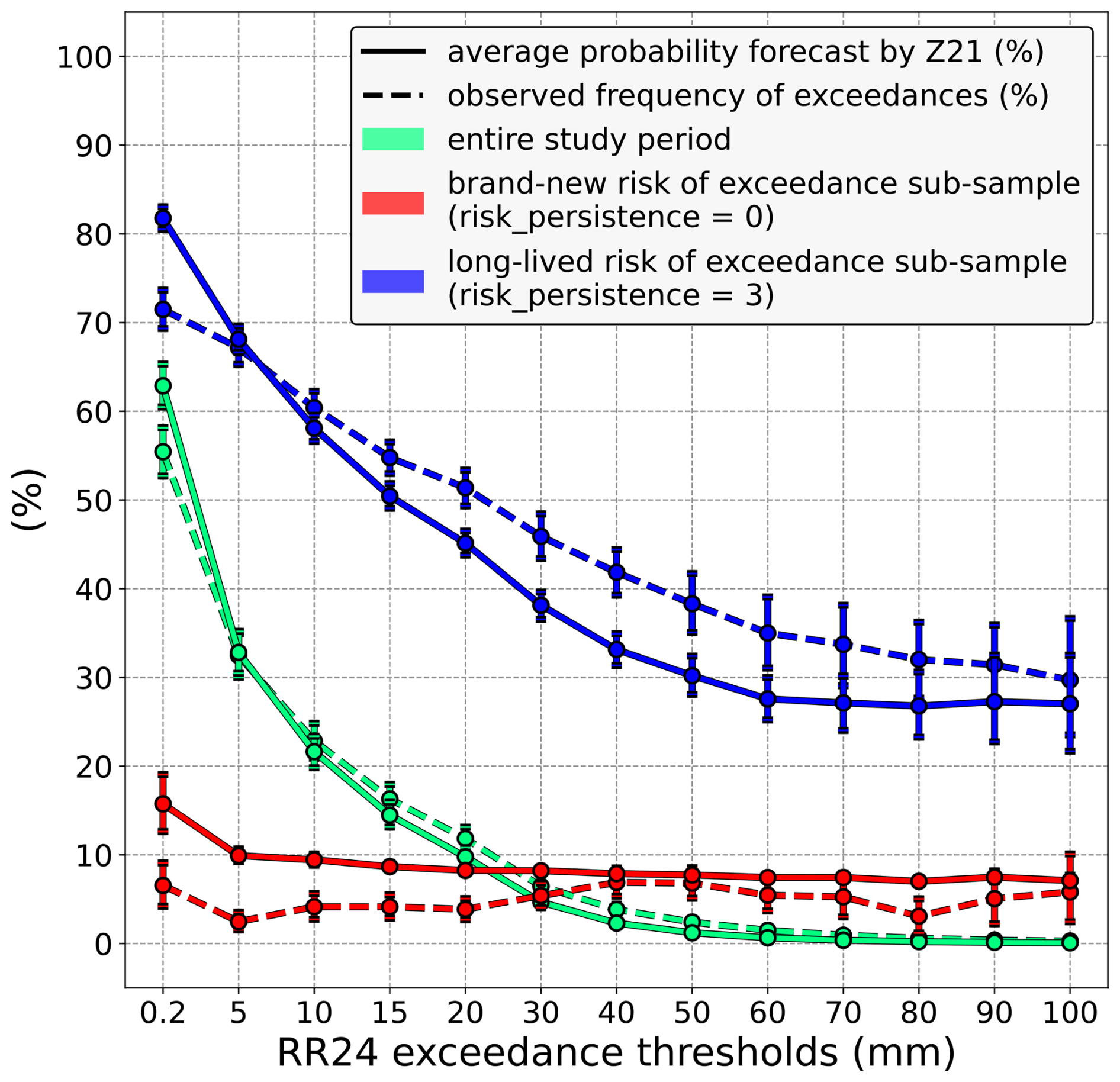
Figure 4 Comparison between the average probability of exceedance predicted by Z21 (solid lines) and the observed exceedance frequency (dashed lines), distinguishing between three different samples. In green, the entire study period is considered. In red, the comparison is restricted to cases where Z21 predicts a brand-new risk of exceedance (risk_persistence = 0), whereas in blue, it is limited to cases where Z21 predicts a long-lived risk of exceedance (risk_persistence = 3). Vertical bars indicate 5 %–95 % confidence intervals.

To assess the practical usefulness of considering how long a risk of exceedance exists, a comparison between the average probability predicted by Z21 (solid lines) and the observed exceedance frequency (dashed lines) is made in the first place and is shown in Fig. 4. This simple diagnostic is used to identify possible trivial under/overestimation biases before conducting any in-depth analysis. This comparison made over the whole study period, regardless of what Z21 predicted or the risk persistence value, leads to the two green lines in Fig. 4. The solid and dashed green lines are close regardless of the precipitation threshold, which means that, on average, Z21 probabilities are a reliable estimate of the risk of exceedance. However, this is not true if this comparison is restricted to cases where a brand-new risk is predicted by Z21 (i.e. risk_persistence = 0, same subsample as in Fig. 3), as depicted by the red lines. In this particular case, the solid line is above the dashed line for most precipitation thresholds, which means that Z21 tends to overestimate the probability of these thresholds being exceeded. On the contrary, when Z21 predicts a risk that has been consistently predicted over the previous runs (i.e. risk_persistence = 3, same subsample as in Fig. 3), the latest run seems to underestimate the probability at most precipitation thresholds (blue lines).

Further analysis is still needed to ensure that the risk persistence explains these biases. Indeed, because the average probability predicted by Z21 is significantly higher when risk_persistence = 3 than when risk_persistence = 0, the previous results could just reflect the fact that high probabilities tend to underestimate the real risk of exceedance, whereas low probabilities tend to overestimate it. An appropriate way of testing this hypothesis is to compute a reliability diagram. Figure 5 shows one related to the 20 mm precipitation threshold for which the under- and overestimations made by Z21 are both statistically significant; see Fig. 4. Focusing on the risk_persistence = 3 case, Fig. 5 confirms that Z21 underestimates the risk of exceedance but only for probability levels under 60 %. For higher precipitation thresholds (not shown), this limit decreases; i.e. only low levels of probability are consistently underestimated. As for the risk_persistence = 0 case, Z21 probabilities are overestimated, but unlike for the risk_persistence = 3 case, Z21 mostly predicts small probabilities, as shown by the frequency histogram (shaded bars; cf. right y axis). This remains true for the other precipitation thresholds (not shown).

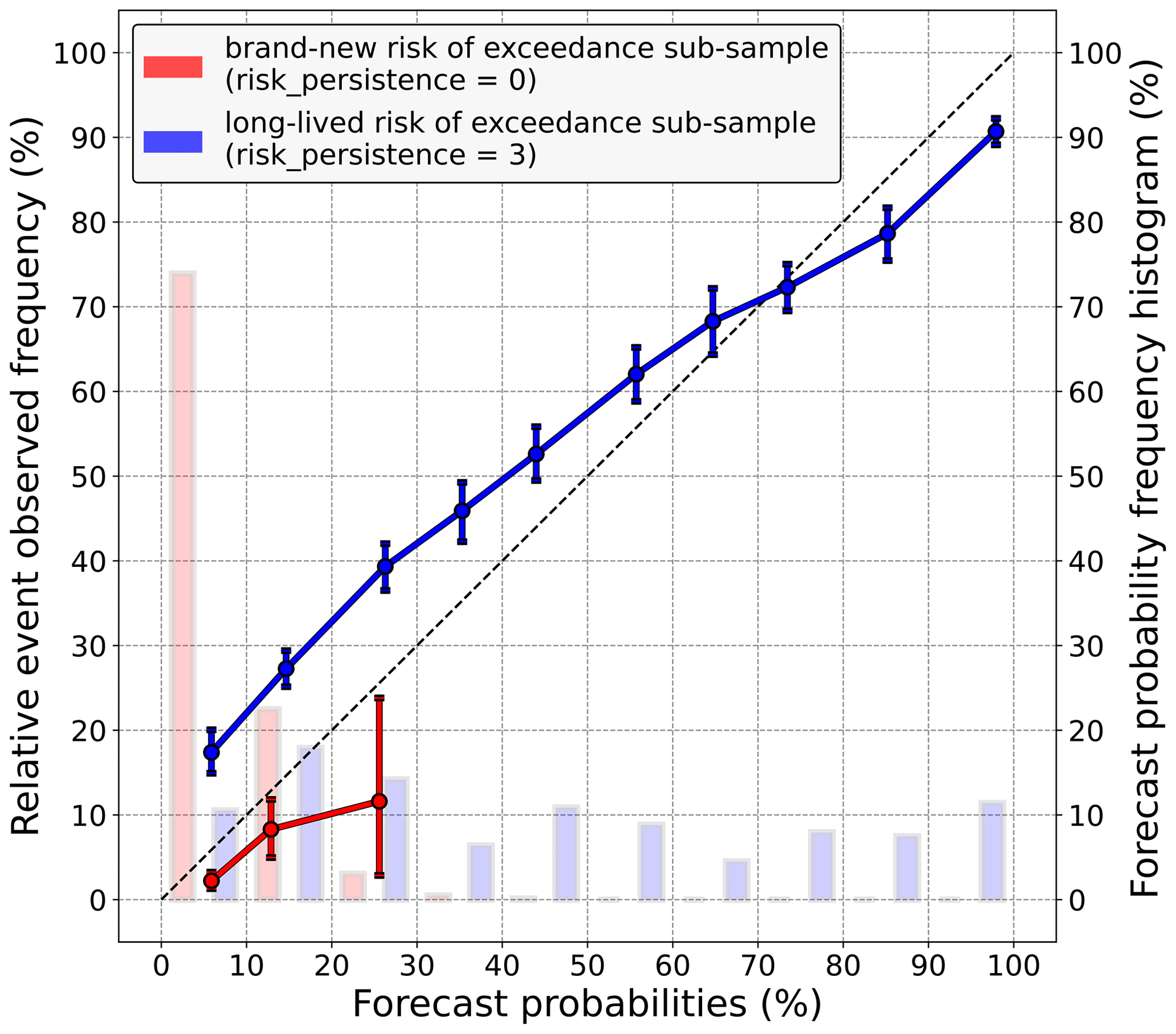
Figure 5 Reliability diagram of Z21 for the 20 mm exceedance threshold, computed over two different samples. In red, only cases where Z21 predicts a brand-new risk (risk_persistence = 0) are considered, whereas in blue, only cases where the risk of exceedance predicted by Z21 is consistent with the three previous runs (risk_persistence = 3) are considered. For each sample, the frequency histogram of probabilities forecast by Z21 is also represented by shaded bars (right y axis). Vertical bars indicate 5 %–95 % confidence intervals.

In this respect, it is interesting to remake the comparison shown in Fig. 4 but on an equal footing, restricting it to only the small probabilities predicted by Z21. Figure 6 illustrates this by focusing the comparison on only Z21 probabilities that are lower than or equal to 15 %. It reveals that when risk_persistence = 3, the low probabilities predicted by Z21 are largely underestimated at all precipitation thresholds, whereas when risk_persistence = 0, these same probabilities are overestimated but to a lesser extent and not for all precipitation thresholds. Also, the underestimation bias when risk_persistence = 3 is much more obvious than in Fig. 4, especially for high precipitation amounts.

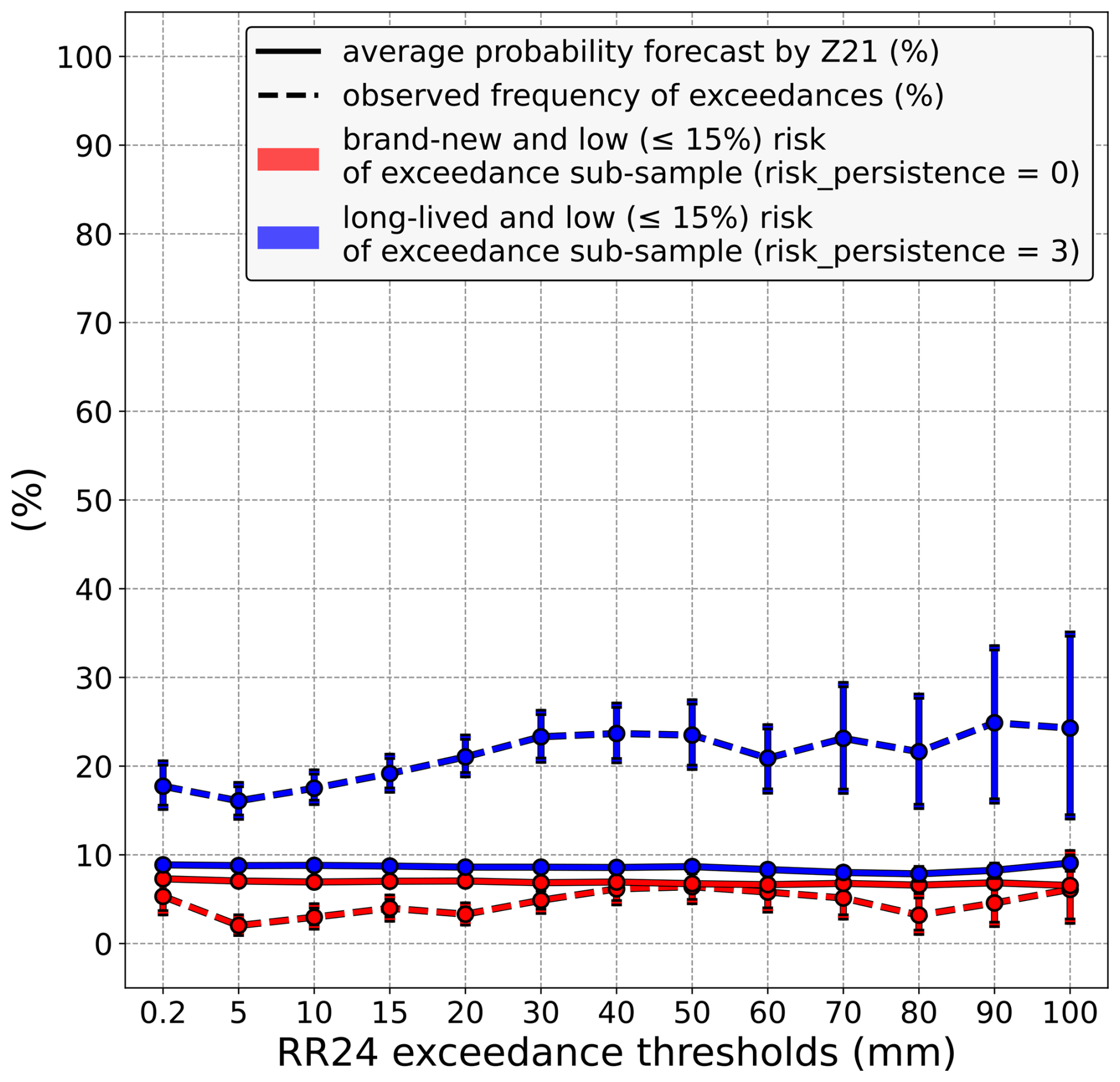
Figure 6 Comparison between the average probability of exceedance predicted by Z21 (solid lines) and the observed frequency of exceedance (dashed lines). Unlike in Fig. 4, this comparison only focuses on low probabilities (≤ 15 %) predicted by Z21. In red, the comparison is restricted to cases where Z21 predicts a brand-new risk of exceedance (risk_persistence = 0), whereas in blue, it is limited to cases where Z21 predicts a long-lived risk of exceedance (risk_persistence = 3). Vertical bars indicate 5 %–95 % confidence intervals.

Some practical recommendations can be made from these findings. If the latest AROME-EPS run predicts a risk of a given precipitation threshold being exceeded in 24 h, forecasters should not take the exceedance probability at face value without checking whether that exceedance scenario has just emerged or has recurred from run to run (possibly in a minority compared to the other members). The probability of this scenario occurring may be overestimated by the latest run in the former case and underestimated in the latter case. In particular, forecasters should pay attention to scenarios that have a small, nonzero probability of occurring according to the latest run but have been repeatedly predicted in previous runs. In that case, their likelihood is probably (largely) underestimated by the latest run. Finally, it should be remembered that the two extreme scenarios of risk persistence are about equally likely to occur when it comes to forecasting heavy precipitation (around 100 mm; cf. Fig. 3). As forecasters should act differently in these two scenarios, they should be particularly vigilant in looking for such events.

These recommendations are valid for forecasters who consider runs separately. Thus, a related question is should a forecaster working with a lagged ensemble ignore such recommendations, or in other words, does the contribution of each run to the final lagged ensemble probability matter? By following the same procedure but using probabilities computed by merging the four daily ensemble runs instead of just Z21, the answer to the last question is also yes, as similar reliability biases depending on the different risk_persistence modalities were found. As evidence, the next subsection will show how the lagged ensemble, as well as Z21, can benefit from the previous results by improving their reliability thanks to the risk persistence information.

4.2 Forecast calibration using the risk persistence information

In this section, the usefulness of risk persistence is assessed using a simple machine learning algorithm, the logistic regression. Doing so, we let an algorithm establish a link between the risk of exceedance and the different risk_persistence modalities and use it to derive enhanced forecasts. In the following, three regressions are tested. The first regression uses only one input variable, the raw Z21 probabilities. The second regression also uses the risk_persistence variable. The third regression works like the second one, but the raw probabilities are taken from the lagged ensemble based on the four daily runs instead of from Z21. Using the entire study period this time (i.e. regardless of what Z21 predicted), these regressions are trained and then compared with each other and with raw probabilities from Z21 and the lagged ensemble. As for the previous results, the reliability is assessed.

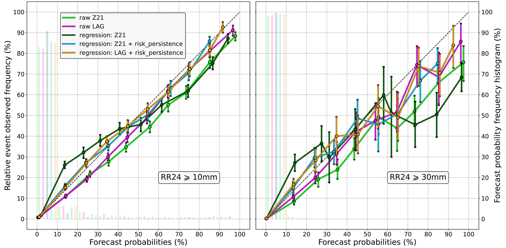
Figure 7 shows reliability diagrams for two daily precipitation thresholds, 10 and 30 mm. Focusing on the 10 mm threshold (left diagram), the latest run and the lagged ensemble (green and purple lines, respectively) are found to be quite reliable, although there is a slight tendency towards probability underestimation. The lagged ensemble is not much better than Z21 and is even worse at the 60 %–70 % levels. The regression with raw Z21 probabilities as the only input variable (dark-green line) performs poorly; it even degrades the reliability of the raw ensemble. On the contrary, reliability is improved with the risk_persistence information (light-blue line). Similar results are obtained with the lagged ensemble (orange line), which demonstrates the usefulness of including the risk persistence information even when using the lagging approach. Focusing now on the 30 mm precipitation threshold (right diagram), the raw ensembles are less reliable. Nonetheless, the regressions that use the risk persistence information still improve the reliability. As for the 10 mm threshold, the regression using raw probabilities as the only predictor performs poorly. Other precipitation thresholds have been tested with similar results, although we must point out that the higher the threshold, the more difficult the assessment, especially for the high levels of probability due to lack of data in the related bins.

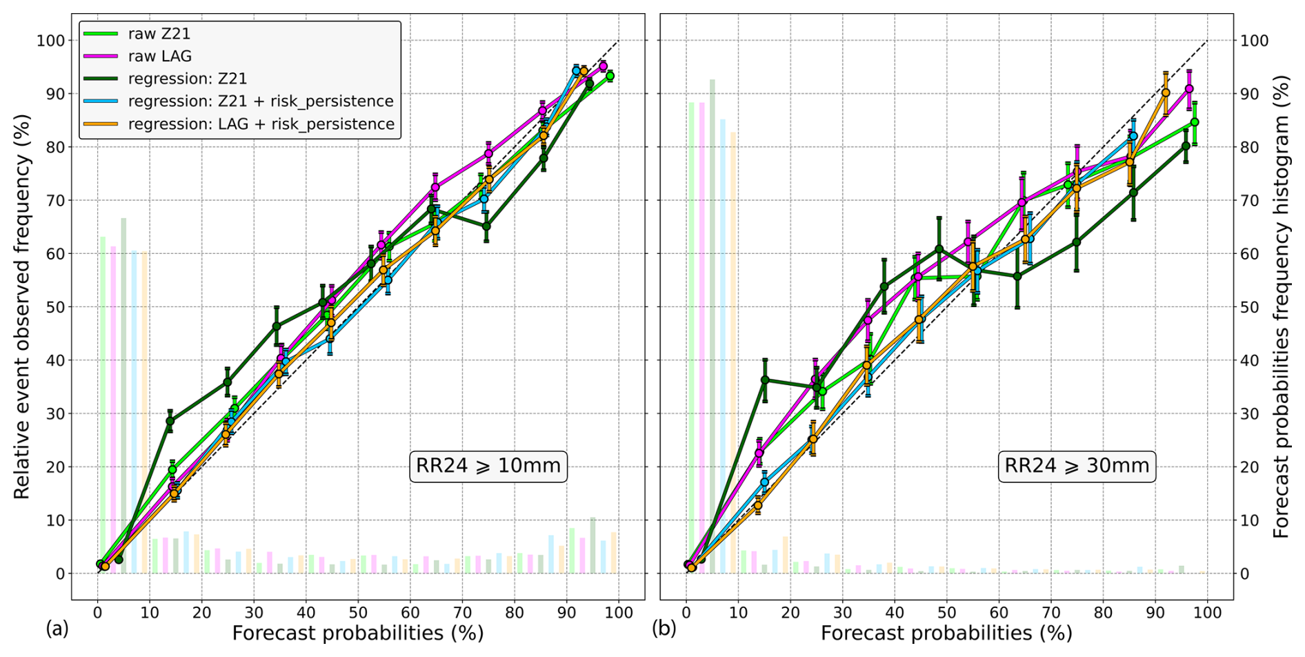
Figure 7 Reliability diagrams for the 10 mm (a) and 30 mm (b) exceedance thresholds. The raw Z21 ensemble is in green, whereas the raw lagged ensemble based on the four daily runs is in purple. The logistic regression with raw Z21 probabilities as only input variable is in dark green. In light blue, the risk_persistence variable is added to that regression. In orange, it is the same regression as in light blue, except that the raw probabilities are derived from the lagged ensemble instead of from Z21. The frequency histograms of the corresponding forecast probabilities are also represented by shaded bars (right y axis). Vertical bars indicate 5 %–95 % confidence intervals.

To understand how reliability has been improved by these simple regressions, it is interesting to visualize how they transform the input raw probabilities, given each risk_persistence modality. Figure 8 shows this dependence for the “blue” regression and for the 30 mm threshold for which the impact of the regression is more obvious. In this figure, each line depicts how the input Z21 raw probabilities (x axis) are transformed by the logistic regression (y axis) within a given risk_persistence case. For example, if risk_persistence = 3 (dark-blue line), a probability of 20 % predicted by Z21 becomes a 30 % probability after the regression. These lines only differ by the specific coefficient affected by the regression to each risk_persistence modality.

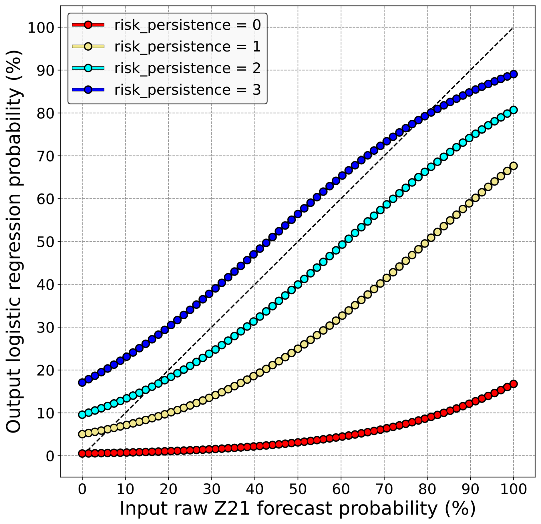
Figure 8 On the y axis, postprocessed probabilities of 30 mm being exceeded in 24 h, derived from the logistic regression with Z21 raw probabilities and risk_persistence as only input predictors. They are expressed as a function of Z21 raw probabilities (x axis), distinguishing each risk_persistence modality (colours).

When risk_persistence = 3, the probabilities forecast by the latest run are increased by the regression, as the dark-blue line is above the diagonal for most probability levels. Also, this upward adjustment of raw probabilities is more important for low levels, even if the difference is small. These results are similar to those shown in the previous subsection, although they were obtained differently. Raw probabilities are adjusted downwards at all the other risk_persistence modalities, the magnitude of this decrease being roughly proportional to the number of previous runs that did not predict a risk. A spectacular decrease is obtained for the risk_persistence = 0 case (red line), for which the regression almost nullifies the latest run regardless of the probability that it predicts. The way raw probabilities are calibrated remains quite the same no matter the precipitation threshold, with only the distance from the diagonal changing slightly (not shown). Fairly comparable results are obtained for the regression with the lagged ensemble, which indicates that probabilities have been similarly calibrated using the risk persistence information, whether they were derived from the last run or from the lagged ensemble.

4.3 Sensitivity of the results to the spatial neighbourhood radius size

As mentioned in the methodology section, all the previous results were obtained using a 25 km radius neighbourhood. What the results would be without any spatial neighbourhood or with a larger one is an important question related to the effective usefulness of this paper. This has been studied by reproducing the results using a 50 km radius neighbourhood and using no spatial neighbourhood at all. In the following, only the impact on the logistic regression is shown because it is a direct assessment of the usefulness of the risk persistence information.

In Fig. 9 the results obtained without any spatial neighbourhood are displayed. In this experiment, the precipitation observations come from all the rain gauges of the RADOME station network (cf. Fig. 1) and the corresponding forecasts from the closest AROME-EPS grid points. Focusing on the 10 mm threshold (left diagram), what differs from the 25 km radius neighbourhood experiment is that raw ensembles are biased in the other sense: raw probabilities, on average, overestimate the risk of exceedance. Nevertheless, reliability is still improved using the risk persistence information, and the regression that does not use it still performs poorly. For higher precipitation thresholds, results cannot really be interpreted because of the large confidence intervals and the jumpy lines, as can be seen in the right diagram (30 mm). This problem does not come from the sample size, which is enlarged compared with the 25 km neighbourhood, as shown in Table 1. Indeed, the larger the neighbourhood, the lower the sample size because fewer verification areas can cover mainland France without any overlap between them. It instead means that there are not enough data points in each probability bin, as shown by the frequency histogram. Very few nonzero probabilities are forecasts, suggesting that it is rare that several AROME-EPS members predict more than 30 mm in 24 h at the exact same grid point. Finally, it should be noted that in this experiment, there is a scale mismatch between observations and forecasts, as we compare regular latitude–longitude gridded forecasts against point observations, which makes the previous results subject to representativeness error (Ben Bouallègue et al., 2020).

Figure 9 As in Fig. 7 but without any spatial neighbourhood.

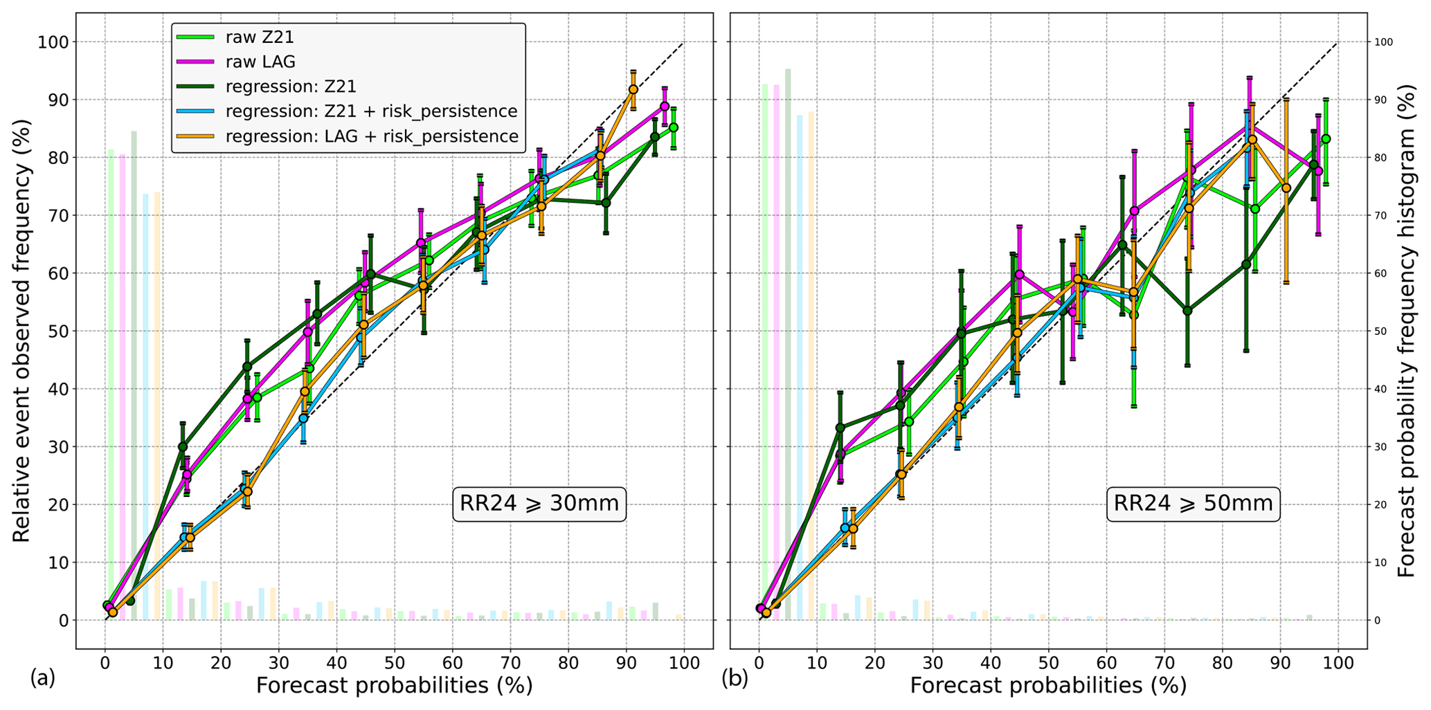
The results obtained with a 50 km radius neighbourhood are shown in Fig. 10. The verification areas used in this experiment can be seen in Fig. A2 (Appendix A), and for comparison purposes, the coverage of both the 25 and 50 km verification areas is displayed in Fig. 1. Because high precipitation thresholds are likely to benefit from upscaling (Ben Bouallègue and Theis, 2013), the 30 and 50 mm exceedance thresholds are assessed. For the 30 mm threshold (left diagram), the reliability bias of the raw probabilities is similar but slightly more exaggerated than in the 25 km experiment. Again, this bias can be reduced using the risk persistence information, in particular for the probabilities up to 30 %–40 %. Similar results are found for higher thresholds, such as 50 mm (right diagram), even if they are only valid for levels up to 50 % due to the lack of data above.

Figure 10 As in Fig. 7 but with a 50 km radius spatial neighbourhood and for the 30 mm (a) and 50 mm (b) precipitation thresholds.

5 Discussion

Several details of this study need to be discussed. To begin with, the risk_persistence definition on which the entire study is based does not fully take into account the chronological order of runs. A more refined definition could be that risk_persistence is equal to

$$\begin{array}{}\text{(4)}& \left\{\begin{array}{ll}\mathrm{0}& \text{if no forecast (Z03, Z09, or Z15) predicted}\\ & \text{a risk}\\ \mathrm{1}& \text{if among Z03, Z09, and Z15, only Z15}\\ & \text{predicted a risk}\\ \mathrm{2}& \text{if among Z03, Z09, and Z15, only Z15 and}\\ & \text{Z09 predicted a risk}\\ \mathrm{3}& \text{if Z03, Z09, and Z15 all predicted a risk}\end{array}\right..\end{array}$$

Compared to the first definition given by Eq. (1), modalities 1 and 2 are more restrictive so as to better characterize the persistence of a given weather scenario, from “brand-new” (modality 0) to “long-lived” (modality 3). Although appealing, this definition suffers from drawbacks that have led us to reject it. The main problem comes from the difficulty of using it as an input variable for a regression because many cases of the risk persistence are not covered, such as “among Z03, Z09, and Z15, only Z09 predicted a risk”. This is problematic within the regression framework since the impact of all these missed cases on the risk of exceedance would be blended into one single coefficient, the intercept, making the usefulness of accounting for the risk persistence more difficult to assess. One solution could be to create as many modalities as there are cases, but each case would represent a small subset, leading inevitably to sample size issues that are harmful to the robustness of the results. In the light of all this, the definition of risk persistence used throughout this study seems to be a good compromise, as it remains quite simple while still providing information about the (in)consistency between runs.

The criterion of “at least one member predicts the exceedance” seems a bit ad hoc and could also be refined. Indeed, the exact number of members simulating exceedance is not accounted for, although it could be a valuable information. We decided to ignore this criterion because it would be too complex for a first study, as it would imply dealing with the many possibilities for the evolution of probabilities over consecutive runs, which could not be summarized by a simple four-modality variable. As an illustration, an overview of the difficulties in characterizing the “trend” feature, i.e. probabilities that increase or decrease from run to run, can be found in McLay (2011). It is also worth saying that beyond the sample size issues this may raise, the definition of such features would be based on probability thresholding, which would need to be adapted to the different precipitation exceedance thresholds. For instance, the “sneak” and “phantom” sequences described in McLay (2011), which are characterized by large and rapid increases or decreases in event probability at short lag times, respectively, cannot be used for high precipitation thresholds in their original definition, since high probabilities of exceedance are almost never forecast at such thresholds. Finally, it should not be forgotten that the entire study is based on AROME-EPS, which only comprises 17 members. Given this ensemble size, the use of statistical quantities such as probabilities can be limited (Leutbecher, 2018). In that context, knowing that something might happen (i.e. that it has a nonzero probability) may already be a strong signal, and knowing the exact value of its probability may be less important in comparison, as already noted by Mittermaier (2007).

Another aspect to discuss is the use of a spatial neighbourhood. In this study, it amounts to introducing a spatial tolerance when forecasts and observations are being compared, as the objective is to predict the probability of daily precipitation exceeding a given threshold anywhere within a given area rather than predicting it at precise locations. Despite this loss of resolution, in our opinion the use of a spatial neighbourhood for precipitation has proved relevant. For instance, without it, we would not know that the risk persistence information could be useful for predicting moderate to high precipitation exceedance. Changing the spatial scale also changes the way different aspects of the forecasts are perceived, which is important to keep in mind. The difference between the frequency histograms of forecast probabilities computed with and without spatial neighbourhoods illustrates this. Because members rarely agree on the exact location of the precipitation amounts, the risk of exceeding them is mostly low without spatial neighbourhoods, and therefore it could appear almost negligible. This impression can be misleading because that same risk is revised upwards as soon as a spatial neighbourhood is introduced, showing that a consensus may appear between the same members at a slightly larger scale. Regarding the neighbourhood size itself, the 25 km radius was chosen because it seemed to be a good compromise. It is wide enough to benefit from the previous advantages while remaining reasonable, especially for Météo-France forecasters who issue warnings at the department scale. Finally, it should be noted that aspects of the spatial neighbourhood other than the radius size could have been investigated but were not, as they were considered beyond the scope of this paper. These could include the sensitivity of the results to the geographical area, the density of the verification zones, the shape of the neighbourhood (for example, squares rather than discs), or the station selection for the 25 and 50 km neighbourhood experiments. Regarding this last point, note that a preliminary study has shown that if we want to keep as many stations as possible while avoiding overlap between verification areas, there are very few possible different samples, probably because some stations are much better at optimizing coverage than others.

If this study focuses on reliability, what about other forecast attributes? In particular, discrimination, i.e. the ability to discriminate between events and nonevents, is also an important aspect of probabilistic forecast (Murphy, 1991). This attribute was investigated using receiver operating characteristic (ROC) curves (Mason, 1982). Surprisingly, discrimination was neither improved nor degraded by incorporating the risk persistence information. In our opinion, it could be a consequence of the specific way raw that probabilities are transformed by the regression. Indeed, an increasing monotonic transformation of probabilities cannot modify the ROC curve, as shown in Jolliffe and Stephenson (2012). Some tests have been carried out to verify this hypothesis, in which interaction terms have been added to the regression: they showed no statistically significant added value in terms of both reliability and discrimination. Understanding why discrimination is not impacted would be a good step forward, as it would better characterize the effective usefulness of the risk persistence information. But it would require further tests, such as using a more advanced machine learning algorithm, which is out of the scope of this paper. In sum, we believe that the (high) sensitivity of the reliability to the risk persistence is already a significant result in and of itself.

Finally, regarding the results themselves, it has to be underlined that they are somewhat at odds with the current state of the art, since the evolution of forecasts has not previously been reported to be strongly related to the upcoming weather. In our opinion, there could be several reasons for this. First, we tried to maximize the chances of obtaining new results on that subject. For example, the present study differs from the previous ones by focusing on a parameter that is well-known for its large spatial and temporal variability and by focusing on a more tangible aspect of forecast evolution than an “all-in-one” run-to-run variability measure. We also felt that working with an ensemble was preferable for the question we wanted to explore. Indeed, the idea behind this work is to find out whether the way the atmosphere is evolving, as perceived by a given NWP system, gives us information about the upcoming weather. For this to have any chance of working, the run-to-run variability has to be an accurate reflection of what is happening in the atmosphere. The problem with deterministic models is that they are nonlinear systems, which are highly sensitive to small perturbations (Leutbecher and Palmer, 2008); therefore, the variations from one run to another, which are assumed to be strictly caused by the assimilation of new observations, may also be insidiously affected by such sensitivity. Ensembles are less subject to this sensitivity by construction and are found to be more consistent from one run to another (Buizza, 2008; Zsoter et al., 2009; Richardson et al., 2020).

Another insight can be found in Richardson et al. (2024). In this paper, the origin of run-to-run variability is studied, and several factors that can influence it are identified and discussed. The data assimilation (DA) algorithm is one of them, and it is clear that changing it would probably affect our results. Independently of this paper, Météo-France is currently testing a three-dimensional ensemble-variational (3DEnVar) DA algorithm (Michel and Brousseau, 2021) for its regional deterministic model AROME-France, and preliminary results show better consistency between runs, in particular for case studies involving heavy precipitation, compared to the current three-dimensional variational (3DVar) scheme (Brousseau et al., 2011). The ensemble spread, size, and perturbations are also important factors identified by Richardson et al. (2024). Whether the same results as ours would be obtained with another ensemble or with a different number of members are interesting and open questions. With a bigger ensemble, the probability of having a weather scenario recurring from run to run would certainly be higher, as each run would explore a wider range of possibilities. In this context, the risk_persistence = 3 case would occur more often, and the risk persistence defined in this study may be of limited use. On the basis of this reasoning, our results can be understood differently. Indeed, it can be hypothesized that if risk persistence has worked for this study, it is precisely because the information that it provides has somehow compensated for the limited size of AROME-EPS by (for example) giving importance back to scenarios whose likelihood was underrepresented for the “wrong” reasons, e.g. not enough members or insufficient sampling of uncertainties (in the lateral-boundary conditions or in the physical parameterizations). If that were true, this study would suggest that limited-size ensembles may suffer from some kind of “memory loss”, which can be partly “healed” by providing a record of their previous runs but in a more subtle way than within the standard lagging approach. Thus, it would finally be in line with the state of the art, as it would mean that it was not the forecast evolution that gave us information on the upcoming weather.

6 Conclusions

This paper addresses the issue of forecasting the weather using consecutive runs of one given NWP system. As forecasts may vary (sometimes significantly) from one run to another, this situation can be difficult to deal with. In the literature, considering how forecasts evolve from one run to another has never proven relevant for the prediction of the upcoming weather. Therefore, the usual approaches to handle this are either considering only the latest run or blending the successive runs all together to create a lagged ensemble. However, both approaches suffer from shortcomings, and if the relationship between changes in forecasts and predictability is assumed to be weak, some aspects remain unexplored. This paper is an attempt to further assess this relationship.

As forecast evolution can be described in many different ways, we have focused on a simple, tangible aspect of ensembles: the persistence of a given scenario over consecutive runs. Following discussions with Météo-France forecasters, we have investigated the idea that the more a scenario recurs from run to run, the more it is likely to occur, but its likelihood is not necessarily estimated as it should be by the latest run alone. Using the regional ensemble of Météo-France, AROME-EPS, and forecasting the probability of certain (warning) precipitation amounts being exceeded in 24 h, the notion of “risk persistence” has been introduced. It characterizes the newness of the weather scenario involving exceedance, from “long-lived” (it was predicted several runs ago and has recurred from run to run) to brand-new (it has just emerged from the latest run) scenarios.

Doing so, we found out that reliability, an important probabilistic forecast attribute, is quite dependent on the risk persistence. In particular, we highlighted that the probability predicted by a given run can be under/overestimated depending on whether or not the previous runs also predicted a nonzero probability. Similar biases were found for the standard lagged ensemble, suggesting that the contribution of each run to the final lagged probability matters. The usefulness of the risk persistence information has also been assessed using a simple machine learning algorithm, the logistic regression. We showed that the forecast reliability can be improved, including for moderate to high precipitation amounts, just by providing it.

In our opinion, what should be remembered about this work is not so much the statistical calibration shown in Sect. 4.2 and 4.3. The important point is instead the high sensitivity of the reliability to something as simple as the risk persistence and the fact that the gain in reliability was achieved by a simple logistic regression, using an unusual type predictor based on previous forecasts. More advanced postprocessing techniques (see Taillardat et al., 2019, and references therein for an overview) would certainly lead to better results. This could be seen as proof that considering forecast evolution can actually be useful for weather forecasting. But it could also reveal that limited-size ensembles may suffer from some kind of memory loss, as they do not reliably estimate the likelihood of weather scenarios that were recurrently suggested by previous runs. Further studies are still needed to better understand this point.

At this stage, we see two applications for this study. It could pave the way for the use of new predictors for statistical postprocessing based on consecutive runs. Indeed, we believe that we can benefit from looking at successive runs in ways other than lagging and that this study is one example among many. It should also discourage operational forecasters from taking raw probabilities at face value without considering their evolution from run to run. Regarding this, it would be very interesting to see if some specific weather phenomena could benefit more from this information than others. For instance, phenomena that are well known for their low predictability, such as Mediterranean heavy precipitation (Khodayar et al., 2021), should be much more feared than more “common” ones if they persist from run to run.

Appendix A: Verification areas for neighbourhood experiments

Figure A1 Verification areas for the 25 km radius neighbourhood experiment.

Figure A2 Verification areas for the 50 km radius neighbourhood experiment.